

Introduction
Remote sensing data is classically acquired from two vectors: satellite and aircraft. The former dataset sampling frequency is limited by availability: the Digitalglobe Image Selection tool (Digitalglobe (2011) provided a maximum of 5 images during the year 2008. We ordered 11 usable FORMOSAT images/year for the 2007–2009 period. While the NOAA POES satellites gather images every 2 hours at latitudes as high as 79°N, and MODIS provides daily coverage (assuming adequate cloud cover conditions), the spatial resolution of such datasets is inadequate for monitoring a 5 km2 glacier. Airborne LIDAR measurement is significantly limited by the availability of the aircraft and associated equipment to gather the aerial imagery, yielding only punctual datasets associated with dedicated programmes.
The present work focuses on complementing satellite based imagery with automated ground based digital camera (Hinkler and others Reference Hinkler, Ørbæk and Hansen2003; Newberry Reference Newbery and Southwell2009; Buus-Hinkler Reference Buus–Hinkler, Hansen, Tamstorf and Pedersen2006; Corripio Reference Corripio2004). Dedicated instruments based on commercially available digital cameras were developed with a frame rate of 3 images/day, limited by design in order to extend battery life expectancy. Post processing focuses on mapping the resulting images in order to obtain compatible datasets from a mosaic of ground based digital cameras and satellite images.
The ground based dataset provides two major improvements: high spatial (10 to 100 cm/pixel side) and time resolution (3 images/day in our case, limited by the power source) in order to provide a continuous survey of a small glacier basin over a minimum of 4 years. The main drawback of this approach is the oblique angle of view which requires significant signal processing to achieve a resulting mosaic comparable with space borne imagery, and the lack of colorimetric calibration of the digital, commercial off the shelf (COTS) cameras.
The field application of this measurement strategy is the basin (10 km2) of a small polar glacier, the Austre Lovénbreen in Spitsbergen (Norway), 6km from the former mining settlement of Ny-Ålesund. This site has been selected for its geological feature of channeling all runoff water from the glacier and the moraine in two rivers, allowing for a continuous monitoring of the water flow rate and an assessment of the contribution of each possible source.
Here, ground based imagery with high spatial and time resolution aims at complementing space borne satellite imagery in order to feed a degree-day glacier melting model, in addition to the interpolated surface temperature measurements from 20 data loggers (Lliboutry Reference Lliboutry1964; Vincent Reference Vincent2002).
Instrument development and available datasets
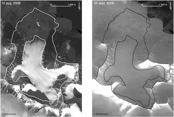
The original dataset we wish to complement for better time and spatial resolution is provided by the FORMOSAT satellite. Its performances set the requirements from the ground based digital camera. FORMOSAT provides daily images at a resolution of 2m/pixel in four wavelength bands ranging from the visible to near infrared, programmable upon user request (Fig. 1).
Two FORMOSAT images acquired from 15 August 2008 (left) and 30 September 2008 (right) exhibit very similar snow cover over the glacier surface due to heavy snow falls days before each picture was acquired, possibly missing some of the heavy melt events as will be seen in this document. No other usable picture has been acquired from this satellite within this time interval due to heavy cloud cover.

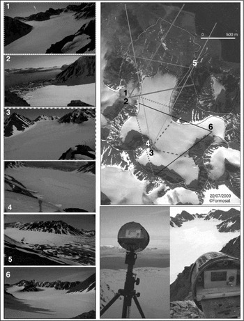
10 instruments were placed on the ridges surrounding the Austre Lovénbreen basin. The locations were chosen in order to cover most of the glacier basin with different view angles in order to minimise the influence of lighting orientation, shadows and poor weather conditions and to provide cross-coverage of most of the glacier surface.
Each instrument is based on a COTS digital camera (either Leica D-Lux4 or Panasonic Lumix LX3; the latter being packaged in a stronger aluminium case is more difficult to modify), selected for its lens optics quality, high sensor resolution (10Mpixel sensors), and data storage on a secure digital (SD) mass storage memory card. Indeed, such a mass storage provides both the bandwidth needed to keep the camera powered for as short a duration as possible (in order to reduce global power consumption) while requiring few enough signals for the card holder to be located away from the camera itself, accessible to the user while keeping the camera in an air tight enclosure (Fig. 2). The camera setting is selected to optimise aperture while automatically adapting the shutter speed to the wide range of lighting conditions met during the polar year.
Positioning of the 6 cameras used to monitor the glacier (the other cameras installed on the glacier basin focus on the moraine), with the field of view of each camera and a typical image captured by each instrument on a sunny day. Bottom right: experimental setup, in which a COTS digital camera is packaged in a waterproof, air tight enclosure. Solar panels complement the lithium batteries for powering the on-board real time clock used for providing the date of each image in the EXIF header.

The digital camera power supply switch and triggering button are controlled by a 4066 analog switch, simulating the manipulation by a human operator. Because of a significant leakage current when the camera is powered, the linear regulator used to supply current to the camera is selected with an enable pin to save battery capacity when the camera is not powered. The drawback of this approach is that the camera real time clock, used to provide the date information in the EXIF header of each picture, powered by an internal manganese accumulator, loses its date and time memory capacity after a duration depending on climatic conditions but ranging from 1 to 3 months. In order to extend this clock memory life expectancy, external solar panels complement the output of the linear regulator through diodes in order to keep the real time clock powered when the sun illumination level allows for a voltage above 5V. Under such conditions, the leakage current is measured to be in the 20mA range.
All sequences, embedded real time clock defining when the camera is switched on, switching on the camera, focusing, triggering the picture capture sequence and switching off the camera, are controlled by a low power Texas Instruments MSP430 microcontroller. The embedded real time clock is software defined: every second the microcontroller wakes up, manages the real time clock and compares its status with a user programmed alarm, and checks the voltage level on a USB input in order to assess whether a user attempts to reconfigure the settings (real time clock or alarm values). The available settings provide the definition of a daily start time, followed by a number of pictures taken daily at pre-defined time intervals. This sequence is repeated every day, minimising the conditions of acquiring pictures in low light conditions.
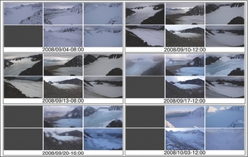
This setup provided a total of about 20000 pictures over a duration of 3 years, out of the expected 32800. The cameras were kept running the whole year at fixed time intervals, even though the images taken during night, full darkness sets from end of November to end of January at this polar latitude, are not usable. Maintenance was performed twice every year, in April and September. Besides some data losses due to erratic electronic circuit behaviour, either water condensation on the printed circuit boards or electrostatic discharge from electric potential buildup associated with snow friction on the insulating casing under strong winds, the number of usable images is limited by weather conditions, as would be the case of visible spectrum satellite imagery. Only the lowest cameras provide usable pictures during overcast days. The setting we used was one image every 4 hours, 3 times every day, starting at 8 AM UTC (Fig. 3). The purpose of this recording setup is to ensure that at least one usable image was acquired every day under most weather and lighting conditions. All these technical choices were directed by reliability, weight and autonomy concerns, yielding successful autonomous acquisitions during 4 years.
Images gathered by the cameras located around the glacier basin from 15 August 2008 to 3 October 2008: each set of 6 pictures is taken at the same time. Only the most relevant datasets were selected in this timeframe.

As mentioned earlier, our purpose is to complement the 2m/pixel FORMOSAT images. We have hence calibrated the pixel size of the digital camera assuming perfect optics (no diffraction), atmospheric conditions (no diffusion) and without including blurring due to the JPEG compression algorithm. Indeed, the cameras we selected do not support a raw storage mode, which would anyway not fulfill our autonomy requirement of storing at least 6 months worth of images or about 540 images, requiring at least 20 GB of storage space which was not available in SD format at the time this programme was started. In addition, the image processing main limitation is due to changing colour as a function of weather and lighting conditions rather than resolution.
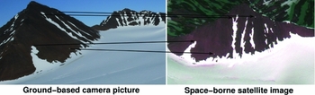
The Leica camera was calibrated to cover an angle of 65° over 4,224 pixels, yielding an angular coverage of 2.7−4rad/pixel, consistent with the nominal focal length of 28 mm equivalent for a 35 mm camera. At such a small angle, one can easily deduce the pixel size by multiplying the distance the scene is located from a camera lens: for a pixel located 1km away, the pixel size is 27 cm wide, and the furthest distance visible from the camera within the glacier basin, located about 5 km away, is associated with a pixel size of 1.35 m, consistent with the resolution of the satellite images. Hence, we conclude that meaningful comparisons between the two datasets are achievable (Fig. 4).
Comparison of one of our ground based camera image (left) and a FORMOSAT satellite image acquired from space (both images acquired on 22 July 2009). Reference points, especially on the foot slope, are selected amongst the natural features for associating coordinates of the satellite-based image and ground based picture.

Digital image processing
The resulting dataset must be processed in order to provide a format consistent with the satellite images. The oblique views gathered from the ground are inadequate in their raw state for quantitative analysis and comparison with the other available datasets.
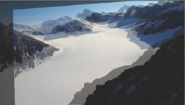
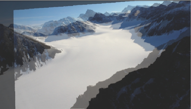
The classical projection algorithms used to map satellite images on a Digital Elevation Model (DEM), as implemented, for example, in the ArcGIS software suite, are inappropriate due to the low viewing angle with respect to the glacier basin (Fig. 5). Such artifacts have already been described (Hinkler and others Reference Hinkler, Pedersen, Rasch and Hansen2002) and are inherent to ground based cameras acquiring oblique view pictures of the landscape.
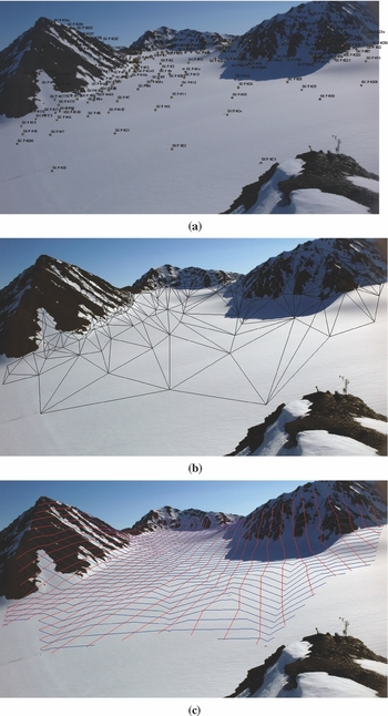
1: Map of the reference points used for the geometric correction for camera number 3. All the points on the glacier surface are 2mx2m flags located using a Coarse/Acquisition (C/A) code GPS, while reference points of the slopes and ridges are visually identified. 2. Each point is paired with a set of pixel identified on one reference picture of each camera, here camera number 3 in the naming convention of Fig. 1. 3. Resulting geometrically corrected image. All processing performed on the images acquired on 22 July 2009.

The proposed alternative is to use a rubber-sheeting geometrical correction model in which oblique pictures are linearly interpolated using Delaunay triangulation. This approach requires the definition of several reference points that both satellite and oblique images have in common. The main difficulty associated with this method is to find features that can be accurately identified on both data sources. Indeed, arctic environments do not display highly featured natural objects but large monotonous regions, either snowy or rocky surfaces are most common. This fact makes the identification of reference points on a glacier difficult or limited to a few structures such as large crevasses or supraglacial stream (bédières). In order to provide artificial reference points, several flag mapping sessions were performed on the field: 2 m × 2 m orange flags were positioned flat on the snow at regular space intervals on the glacier surface so that each camera captured images on which each geolocated flag could be associated with a pixel position on the picture. These flag sessions were complemented with a few manually triggered images of an operator riding a skidoo on the glacier, each position being again geolocated using a Coarse/Acquisition (C/A) code GPS. Eventually, geographic reference points (ridges, mountain summits, rock/snow interfaces), including the slopes which exhibit features easy to identify as control points, were added to the reference point database in order to restrict the correctly rectified area to the glacier surface and close neighbourhood.
An additional challenge stems from the multiple maintenance sessions: twice a year, on which the batteries are changed, and in case of major dysfunction, the whole camera is replaced with a spare setup. In such a procedure, considering the high image resolution yielding sub-m pixel size over the glacier basin, some image motion is unavoidable. Hence, images acquired at various nearby orientations are corrected to match the reference picture using a two-dimensional second order polynomial fit defined by some manually selected geographic features (Fig. 6).
Comparison of two images taken by the same camera, before and after maintenance sessions yielded camera motion. Since the camera lens is still positioned at the same point after putting the camera back on its holder, a 2D second-order polynomial distortion is used to associate far-away (ridge, fjord) and nearby stable (rock) features in order to provide a consistent dataset over the 4 year acquisition period. All images must be centered identically for the reference points located on the field and on a reference image to be applicable.
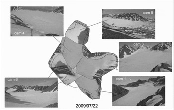
Having geometrically rectified all images, they are mapped on the surface defined by the Delaunay triangles (Fig. 7), which have been defined using the reference points (artificial flags, natural features such as ridges and moraine). The resulting 2D-zenithal projection views of all pictures are then assembled as a mosaic to provide a complete coverage of the whole glacier as presented in Fig. 8 for one particular dataset, all pictures being acquired at the same time and date. Since the purpose of this mosaic is a quantitative analysis in comparison with satellite images, aimed at identifying the fraction of the glacier covered with either ice or snow (binary information), no white balance adjustment or histogram equalisation between the various pictures forming the mosaic have been performed.
From left to right: identification of the position of the reference points both on the DEM and on one of the pictures; Delaunay triangulation using these reference points as vertices; finally, linear interpolation of each pixel position within each triangle.

Mosaic and field of view of each camera. A few areas of the glacier basin are not covered due to constraints in safely accessing the sites where the cameras are located on the ridges in any season during the field trips. Over 96% of the glacier basin area is covered by the picture mosaic. Compare with the result of a geometric projection on a DEM as shown in Fig. 5.

The result of these processing steps is a mosaic of images projected over a glacier basin model using a rubber sheeting strategy which yields consistent results with the images gathered from satellite, enabling a quantitative analysis of both datasets for comparison (Fig. 8). The surface coverage from the ground based camera is 96% of the glacier, with the missing parts due to some blind spot effect from some of the mountain slopes which are not compensated for by overlapping field of views from various cameras in the deepest cirques.
Results and discussion
As an example of results achieved by this measurement strategy, we focus on a heavy rainfall event over a short time period (9–23 September 2008), inducing significant melt over the whole glacier. This sudden event totaled 76% of the summer precipitation, is the cause of 40% of the summer runoff, and contributed 71% of the annual ablation.
From the two consecutive FORMOSAT images we gathered, which encompasses all the usable data acquired from this satellite within the time interval 15 August 15 to 30 September 2008 (Fig. 1), one might have deduced that the glacier was fully covered with snow throughout the period ranging from mid-August to the end of September 2008. Such an assumption would have missed the strong flood event, due to the association of elevated temperatures combined with rain, observed from the ground based cameras between 11–19 September. Furthermore, assuming a constant snow coverage would have led to an underestimate of the melt rate due to an overestimate of the ground albedo.
Indeed, one reason for our need for high spatial and time resolution of the glacier state is for the application of a degree-day melting model, the input of which is the ground temperature distribution over the glacier basin and ground albedo (Braithwaite Reference Braithwaite1984; Johannesson and others Reference Johannesson, Sigurdsson, Laumann and Kennett1995; Zhang and others Reference Zhang, Liu and Ding2006). Hence, the series of pictures from the glacier, projected in an UTM compatible vertical view, provide the raw data for ice/snow limit delineation and for assessing the hydrological budget of the glacier at high spatial resolution and with sub-week time intervals. It also allows for the identification of fast events such as sudden (<1 week long) floods associated with short climatic events (temperature increase, rain) that significantly contribute to the glacier mass balance. Eventually, the binary information of snow or ice cover provides the information necessary to apply the appropriate melting coefficient in the degree-day model. A different coefficient is used for snow covered or bare-ice glacier areas. The final step of the model consists in defining the dynamics of each part of the glacier and at each time step as a combination of the glacier surface condition and the atmospherical thermal state of the glacier resulting from hourly temperature measurements recorded by 20 automated probes distributed on the glacier.
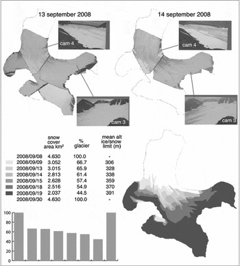
Furthermore, under most conditions, only a subset of the available images is needed to identify the snow-ice limit, since the snow melt is usually a slow event with an altitude limit observed by only a few of the installed cameras (Fig. 9). The acquisition of 3 images every day improves the chances of good weather condition and sun position for appropriate illumination allowing for the manual identification of the snow covered areas of the glacier. Due to the poor contrast and varying colours with weather conditions, only a visual selection of the useful images and the snow covered areas allows for an accurate estimate of the snow-ice boundary. All automatic identification attempts failed due to the poor colour content, defeating unsupervised or supervised classification strategies, such as principal component analysis. This manual boundary identification is applicable since only a few days of significant melt are observed over a whole season, with only a few melting jolts.
Mapping the snow and ice covered areas of the glacier using the zenithal projection of the picture mosaic: the ice-snow limit is identified and drawn manually under ArcGIS, since automated identification under variable illumination angle and cloud conditions seems challenging using only visible wavelength imagery. In some instances, only a subset of the available cameras is used since the ice-snow limit is continuously visible on the resulting mosaic assembly. Bottom-left: graphical view of the evolution of the snow coverage as a function of time of the dates provided in the table above.

Conclusion
We installed 10 instruments around a small (10 km2 large) arctic polar glacier basin (79°N, Svalbard, Norway) based on commercial digital cameras for acquiring pictures of the glacier 3 times per day at regular time intervals. The resulting datasets are used as a complement to space borne satellite imagery, providing higher spatial resolution with respect to the FORMOSAT dataset we obtained between 2006 and 2010, and higher sampling rate (3 times per day as opposed to one satellite image every month, limited by weather conditions), once the mosaic has been projected to a format compatible with the zenithal projection.
The challenges of processing oblique view images are described, using a Delaunay triangle map supported by reference points to avoid the pitfall of diverging points far from the camera lens when using solely a projection on a digital elevation model of the glacier. The resulting binary information concerning the fraction of the glacier surface covered with snow or ice is used as input to a degree-day model in which the melting coefficient is dependent on this property. The resulting dataset will now allow assessing the hydrological budget of the glacier by including the detailed snow coverage area of the glacier in a degree-day melting model.