Extinction in the Fossil Record
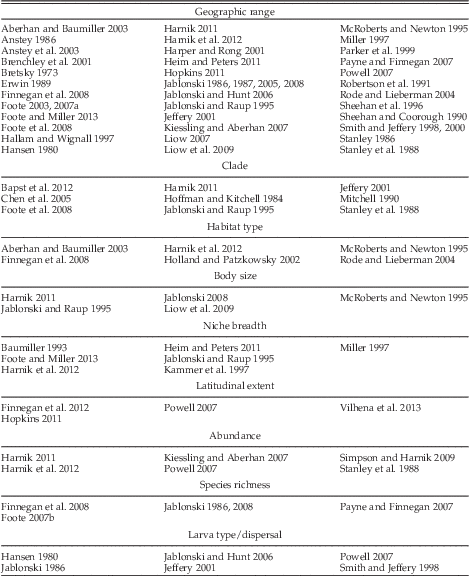
Extinction has always been a topic of great interest in the field of paleontology but only in recent decades have large-scale quantitative analyses of extinction and the factors that make organisms vulnerable to extinction become common. This change reflects the compilation of online databases, such as the Paleobiology Database, which have aggregated thousands of occurrences from the published literature and curated collections around the globe. Investigations have identified a large number of factors associated with extinction risk across many clades (Table 1). Of all the properties associated with extinction risk (or its inverse, species duration), only geographic range is a consistent factor across times of both background and mass extinction and across a large number of clades (e.g., Jablonski Reference Jablonski1986, Reference Jablonski2005, Reference Jablonski2008; Erwin Reference Erwin1989; Boyajian Reference Boyajian1991; Jablonski and Raup Reference Jablonski and Raup1995; Payne and Finnegan Reference Payne and Finnegan2007; Powell Reference Powell2007; Harnik Reference Harnik2011; Finnegan et al. Reference Finnegan, Heim, Peters and Fischer2012). All but a few of these studies have focused on shelly invertebrates, however, which no doubt reflects their comparable contribution to the marine fossil record. Thus, the generality and, to a considerable degree, the cause of this dependence of extinction risk on geographic range remains unclear.
Factors correlated with extinction risk in the fossil record and their references.

Just as the observed changes in the diversity of marine animals over the course of the Phanerozoic may be driven in part by the availability of fossil-bearing formations (Raup Reference Raup1972; Peters and Foote Reference Peters and Foote2001; Peters Reference Peters2006; Smith and McGowan Reference Smith and McGowan2007; Wall et al. Reference Wall, Ivany and Wilkinson2009; but see Dunhill et al. Reference Dunhill, Hannisdal and Benton2014), one must also consider whether calculations of geographic range may be influenced by sampling. The overall likelihood that a species is recovered from a rock unit (i.e., is sampled) depends on the cumulative effects of a species’ original abundance, ecology, taphonomy, and collection effort. We return below to a discussion of the particular components of sampling encompassed in this study. The covariation between sampling and geographic range has been difficult to disentangle because taxa with large geographic ranges are expected, even by chance, to be observed more often than taxa with small geographic ranges (Russell and Lindberg Reference Russell and Lindberg1988; Gaston et al. Reference Gaston, Quinn, Wood and Arnold1996). Only a few studies have attempted to control for sampling in studies of extinction risk, and these are discussed in more detail below (“Geographic Range and Sampling”). Those studies that have controlled for some of the components of sampling generally found that geographic range remains a significant predictor of extinction risk but rarely discuss the relative strength of sampling versus geographic range. Thus, the relationship between these two factors remains uncertain.
Part of the reason for this uncertainty is that most studies are constrained by the trade-off between taxonomic, temporal, and spatial resolutions inherent to databases built from collections that were never expected to be used in such analyses. For example, temporal resolution is usually at the stage or substage level, which can artificially expand taxon durations (Holland and Patzkowsky Reference Holland and Patzkowsky2002; Foote Reference Foote2003, Reference Foote2007a). Related to this, analyses typically use genera or higher-level taxa as their units of investigation despite the fact that selection for properties such as geographic range are expected to take place at the species level (Gaston and Fuller Reference Gaston and Fuller2009). Higher-order taxa are widely used in paleobiological studies because species-level taxonomic assignments are often questionable or unavailable and most species have short durations compared with the temporal resolution available for the analyses. Additionally, for a given level of sampling effort, the completeness of sampling (i.e., the proportion of originally present taxa included in the sample) increases as one moves up the taxonomic hierarchy. Error arising from these issues can be reduced by focusing on particularly well-studied regions and taxonomic groups (Erwin Reference Erwin1989; McRoberts and Newton Reference McRoberts and Newton1995; Rode and Lieberman Reference Rode and Lieberman2004; Heim and Peters Reference Heim and Peters2011; Hopkins Reference Hopkins2011; Finnegan et al. Reference Finnegan, Heim, Peters and Fischer2012). We use a species-level, global database of planktic graptolites to produce a finely resolved temporal, taxonomic, and spatial analysis of extinction risk.
The graptolite database contains 1114 taxa drawn from the group’s entire 80 Myr history and was used to construct the early Paleozoic timescale (Cooper and Sadler Reference Cooper and Sadler2012; Melchin et al. Reference Melchin, Sadler, Cramer, Cooper, Gradstein and Hammer2012). The timescale was formed by an ordination technique called CONOP (Sadler et al. Reference Sadler, Kemple and Kooser2003, Reference Sadler, Cooper and Melchin2009), which allowed for durations of species to be calculated from a continuous, time-scaled sequence. This approach entirely avoids the necessity of time binning. We employ the same database here to 1) quantify and examine the covariance of geographic range and sampling in relation to extinction risk; 2) test whether, after controlling for covariation between sampling and geographic range, either has any independent predictive power in relation to extinction risk; and 3) test whether graptolite-specific factors such as biofacies groups, clade, and particular intervals of geological time are significant predictors of extinction risk, while also assessing their strength relative to more general properties, such as geographic range.
Factors Correlated with Extinction Risk
As noted above, many factors have been associated with extinction risk, but the link to geographic range is by far the most widespread and consistent across studies (Jablonski Reference Jablonski2005; Kiessling and Aberhan Reference Kiessling and Aberhan2007; Harnik Reference Harnik2011). Geographic range can be measured by a variety of methods, including counts of regions (Foote Reference Foote2003; Finnegan et al. Reference Finnegan, Payne and Wang2008), linear distances (Powell Reference Powell2007; Harnik Reference Harnik2011), or areal measures (Foote and Miller Reference Foote and Miller2013; Dunhill and Wills Reference Dunhill and Wills2015). Each of the different measures has advantages and drawbacks (Gaston and Fuller Reference Gaston and Fuller2009), and there is no single measure that presents an objectively more accurate representation of species’ geographic range than other measures. Besides being measured in disparate ways, the meaning of geographic range is difficult to interpret, since it is tightly correlated with both sampling and species’ ecology (Brown et al. Reference Brown, Stevens and Kaufman1996). Attempts to assess the influence of sampling as an independent factor have measured it either as the number of occurrences (Smith and Jeffery Reference Smith and Jeffery1998; Payne and Finnegan Reference Payne and Finnegan2007; Hopkins Reference Hopkins2011; Harnik et al. Reference Harnik, Simpson and Payne2012; Boyle et al. Reference Boyle, Sheets, Wu, Goldman, Melchin, Cooper, Sadler and Mitchell2014) or the proportion of possible occurrences in a taxon’s duration (Finnegan et al. Reference Finnegan, Payne and Wang2008; Foote et al. Reference Foote, Crampton, Beau and Cooper2008). The number of occurrences, however, has itself been interpreted as a measure of geographic range (e.g., Jablonski Reference Jablonski1986; Jablonski and Hunt Reference Jablonski and Hunt2006). The proportional approach has the additional problem of counting absences as informative, because even collections made at sites in the wrong biofacies within a taxon’s duration are generally included in the calculation.
Although geographic range and sampling are consistent factors that impact extinction risk, particular intervals in Earth’s history also have had different extinction rates. The most extreme differences between time periods are represented by mass extinction versus background extinction, which often have stark differences in the significance or at least the strength of factors associated with extinction (Erwin Reference Erwin1989; Boyajian Reference Boyajian1991; Payne and Finnegan Reference Payne and Finnegan2007; Jablonski Reference Jablonski2008; Finnegan et al. Reference Finnegan, Heim, Peters and Fischer2012; Cooper et al. Reference Cooper, Sadler, Munnecke and Crampton2014). In some mass extinctions, the normal association between geographic range and extinction risk appears to have broken down (McRoberts and Newton Reference McRoberts and Newton1995; Smith and Jeffery Reference Smith and Jeffery1998; Stanley et al. Reference Stanley, Wetmore and Kennett1988; Jeffery Reference Jeffery2001; Kiessling and Aberhan Reference Kiessling and Aberhan2007; Foote et al. Reference Foote, Crampton, Beau and Cooper2008). Even intervals outside those normally regarded as mass extinctions (i.e., intervals of so-called background extinction) may also differ significantly from one another in extinction risk, as exemplified by the drop in both average extinction and origination rates over the course of the Phanerozoic (Raup and Sepkoski Reference Raup and Sepkoski1982; Alroy Reference Alroy2008; Goldman et al. Reference Goldman, Bergström, Sheets and Pantle2013a). Thus, we need to consider the role of changing extinction regime over the course of our studied intervals.
Differences between background extinction intervals might be driven by differences between clades as faunas are replaced. Modern taxa have been shown to vary greatly in extinction risk based on the ecology of their particular clades (Foden et al. Reference Foden, Butchart, Stuart, Vié, Akçakaya, Angulo, DeVantier, Gutsche, Turak, Cao, Donner, Katariya, Bernard, Holland, Hughes, O’Hanlon, Garnett, Şekercioğlu and Mace2013), and this has been shown in fossil organisms as well (Aberhan and Baumiller Reference Aberhan and Baumiller2003; Cooper and Sadler Reference Cooper and Sadler2010; Harnik Reference Harnik2011). However, there has been relatively little work on the ecological differences among fossil organisms, because they are less generalizable and more difficult to measure than geographic range. It is also worth noting that analyses of extinction have been dominated by benthic marine invertebrates as a consequence of their high preservation potential. These taxa represent only a small fraction of the modes of life occupied by organisms, and there is little reason to expect that the extinction risks of organisms with vastly different lifestyles (e.g., terrestrial, volant, planktic) will be influenced to the same degree by the factors that affect benthic taxa.
Graptolite Paleoecology
Planktic graptolites are a well-studied clade of metazoans, fossils of which are used extensively in biostratigraphy. These organisms were colonial macrozooplankton that occurred abundantly through the Ordovician and Silurian periods and persisted into the lower Devonian (485−411 Ma) (Cooper et al. Reference Cooper, Rigby, Loydell and Bates2012). Graptolites also represent the earliest substantial record of oceanic zooplankton and make ideal fossils for biozonation, because species were short-lived compared with other taxa and tend to be very widespread (Sadler et al. Reference Sadler, Cooper and Melchin2009). This makes the group particularly interesting in extinction studies as a contrast to benthic invertebrates, which typically have smaller geographic ranges but can persist for long periods by tracking environments. The widespread geographic range of many graptolite species might limit the impact of variable geographic range on extinction risk and allow for easier detection of other graptolite-specific factors.
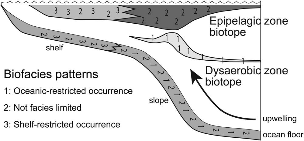
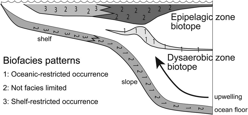
One such factor that has been associated with extinction risk in graptolites is biofacies groups. It has long been recognized that graptolites fall into at least two broad categories based on their distributions in different depositional settings (Berry Reference Berry1962; Erdtmann Reference Erdtmann1976; Fortey and Cocks Reference Fortey and Cocks1986). This hypothesis has been formalized with the recognition of three biofacies groups (Cooper et al. Reference Cooper, Fortey and Lindholm1991; Cooper Reference Cooper1999). Group 1 species are confined to sediments deposited in deep-water, open oceanic settings (ocean-restricted), group 2 species occur in both deep sediments and in relatively shallower, shelf sediments (unrestricted), and group 3 species occur only in sediments deposited in shelf settings (shelf-restricted). These groups have been interpreted as a consequence of an original depth and water mass zonation of graptolite habitats in the water column (Fig. 1). In this model, group 1 species occupied a mesopelagic habitat and used the oxygen minimum zone (Cooper and Sadler Reference Cooper and Sadler2010; Cooper et al. Reference Cooper, Rigby, Loydell and Bates2012), an area of high productivity but low oxygen that today hosts a unique fauna of specialist invertebrates (Mullins et al. Reference Mullins, Thompson, McDougall and Vercoutere1985; Levin Reference Levin2003). Group 2 species dwelt in the epipelagic oxic water depths where taxa could thrive on other planktic organisms. Group 3 is a relatively small group of graptolites that were endemic to the vast epicontinental seas that covered much of the continents during the Ordovician and Silurian periods.
Distribution of graptolite biofacies groups and the inferred location of graptolite biotopes along a continental margin. Modified from Cooper and Sadler (Reference Cooper and Sadler2010).
Methods
Data Collection
Taxa and Durations
All graptolite taxa analyzed were drawn from those used for calibrations for The Geologic Time Scale 2012 (Cooper and Sadler Reference Cooper and Sadler2012; Melchin et al. Reference Melchin, Sadler, Cramer, Cooper, Gradstein and Hammer2012) for the lower Paleozoic using the program CONOP9 (Sadler et al. Reference Sadler, Kemple and Kooser2003, Reference Sadler, Cooper and Melchin2009). CONOP is an ordination procedure that automates and elaborates on the graphic correlation method of Shaw (Reference Shaw1964). The program uses the first appearance datum (FAD) and last appearance datum (LAD) of taxa recorded in stratigraphic sections. The result is a time-ordered series of FADs and LADs for all taxa in all sections. This ordination is then scaled to absolute ages using radiometrically dated beds and a fitting procedure that interpolates the age of each event in the composite sequence. From this time-scaled composite the durations of each taxon can be calculated continuously, rather than estimating durations based on time bins. Previous work using this composite calculated extinction rates to examine changes in extinction regime during the Late Ordovician mass extinction event (LOME; Crampton et al. Reference Crampton, Cooper, Sadler and Foote2016). However, calculating extinction rate from durations requires time-binning the data and assuming the extinction is constant within those time intervals, thus introducing biases (Stanley Reference Stanley1979; Foote Reference Foote2000). Here, we chose to use the continuous nature of the data set and used taxon durations directly as a proxy for extinction risk, the likelihood of extinction. Because durations are inversely related to extinction risk, the correlations between duration and factors that influence extinction risk are easily interpreted and visualized (i.e. Jablonski Reference Jablonski2005: Fig. 1; Kiessling and Aberhan Reference Kiessling and Aberhan2007: Fig. 5). For the purpose of the analyses described below, the variance in extinction risk refers to the variation in the calculated durations of taxa.
For the 2012 Geological Time Scale, Cooper and Sadler (Reference Cooper and Sadler2012) and Melchin et al. (Reference Melchin, Sadler, Cramer, Cooper, Gradstein and Hammer2012) employed 512 stratigraphic sections from across the globe that spanned the Ordovician to the Lower Devonian. Several of these sections were themselves regional composites of many individual sections. They included a total of 2045 taxa, but nearly half of these occur in only a single section or composite. Taxa seen in few sections tend to have a large degree of uncertainty associated with their calculated durations in CONOP (Sadler et al. Reference Sadler, Cooper and Melchin2009) and only introduce noise into analyses of extinction risk. Therefore, we analyzed geographic range data only for the 1114 taxa in this data set that are known from more than one section. The taxonomic validity of records for some of the taxa have been vetted, but the majority of the taxa included in our analyses have been taken directly from the original literature without editing except in clear cases in which a senior synonym or new generic identification is available or where disjunct occurrences in the composite sequence suggest the conflation of distinct taxa (see Sadler et al. Reference Sadler, Cooper and Melchin2011: p. 337). All of the taxa included for analysis are species or subspecies and a few are in open nomenclature (e.g., Corymbograptus cf. deflexus) where the name appears to have been used in a consistent sense by an author.
Geographic-Range Measures
Geographic range has been identified previously as having a strong correlation with extinction risk, dominantly in benthic organisms, which tend to be less widespread than graptolites. Therefore, the strength of the correlation between geographic range and extinction risk in a widespread planktic group is of great interest in macroevolution. However, there is little agreement on how to best measure geographic range in modern groups (Gaston Reference Gaston1994; Gaston and Fuller Reference Gaston and Fuller2009), which present fewer data biases than fossil organisms. To reduce the biases that may be introduced by any single measure of geographic range, we employed seven different methods. Four measures are linear distances: latitudinal range, longitudinal range, maximum pairwise distance, and summation of a minimum spanning tree. We also employed the convex hull, which is an areal measure; the number of paleogeographic regions occupied; and the number of paleogyres occupied, which are counts. Linear and areal measures were calculated in kilometers and kilometers squared, respectively, except for latitudinal and longitudinal ranges, which were measured in degrees. The longitudinal distance was measured as (360 − largest longitudinal gap) to account for taxa that stretched around more than half the Earth. We did not make a similar correction for maximum pairwise distance or convex-hull area calculations. For the 220 taxa with such large ranges (approximately one in five species) this may be an additional source of noise in the maximum pairwise distances and convex-hull areas. As with other aspects of geographic range, latitudinal and longitudinal ranges may have biological meaning beyond their use as proxies for geographic range. Latitudinal range correlates strongly with thermal tolerance in some modern groups (Addo-Bediako et al. Reference Addo-Bediako, Chown and Gaston2000; Sunday et al. Reference Sunday, Bates and Dulvy2011), and longitudinal range has been linked to dispersal capability, although the significance of the correlation is not consistent (Lester and Ruttenburg Reference Lester and Ruttenburg2005; Lester et al. Reference Lester, Ruttenburg, Gaines and Kinlan2007).
To calculate all measures of geographic range for each taxon, we compiled current latitude and longitude coordinates for the 512 studied stratigraphic sections based on data given in the original papers or by estimating those coordinates from their locality maps using Google Earth. Points were transformed to their paleo-coordinates in the program PaleoGIS (Rothwell Group 2007). Uncertainty in the placement of paleocontinents and differences between paleogeographic models (Rothwell Group 2007; Torsvik and Cocks Reference Torsvik and Cocks2013) are much greater than the errors associated with the modern coordinates, even those estimated from Google Earth, which in our tests differ from stated locations in the papers by less than 1 degree.
Several localities, especially those in Alaska and New Zealand, were placed manually in the paleogeographic reconstructions because they were close to terrane boundaries and their current locations did not appear in PaleoGIS reconstructions. Alaska is currently near the edge of a plate boundary and has been tectonically deformed, so points were moved to the nearest terrane that did appear in reconstructions. The repositioning of these points was very small compared with the uncertainty in paleoplate positions. The New Zealand sections could not be moved to a nearby terrane, and it appears that New Zealand is largely absent from the early Paleozoic paleoplate reconstructions of PaleoGIS. Rather than discard these localities, we placed these sites at the boundary between Antarctica and Australia along the northeastern Gondwanan margin based on our knowledge of the fauna and paleogeographic history of the region (R. A. Cooper unpublished data). This placement is in agreement with the paleo-reconstruction of Torsvik and Cocks (Reference Torsvik and Cocks2009, Reference Torsvik and Cocks2013). Composite sections constructed from multiple measured sections, spot localities, or both were treated differently from single sections. Each composite was described as a four-sided polygon that encompassed the stated region from which the original samples were drawn, and all the taxa present in the composite were counted as present at each of the four corner “sites” for the purpose of calculating geographic range. One of the 27 composite sections included in the CONOP composite of Cooper and Sadler (Reference Cooper and Sadler2012) and Melchin et al. (Reference Melchin, Sadler, Cramer, Cooper, Gradstein and Hammer2012), the Polish composite (Teller Reference Teller1969), stretched across multiple paleoplates and thus was not used for geographic-range calculations.
Because PaleoGIS only has reconstructions for the lower Paleozoic in 10 Myr intervals, the reconstruction interval closest to the midpoint of a species’ duration was used to calculate its geographic range. This is not expected to introduce bias, as previous studies have found that many taxa achieve their maximal geographic distribution near the midpoint of their durations (Foote Reference Foote2007b; Foote et al. Reference Foote, Crampton, Beu, Marshall, Cooper, Maxwell and Matcham2007; Liow and Stenseth Reference Liow and Stenseth2007). However, during some intervals of Earth’s history and in some particular groups, taxa may reach their peak geographic range before the midpoints of their durations (Foote Reference Foote2007b; Kiessling and Aberhan Reference Kiessling and Aberhan2007; Liow and Stenseth Reference Liow and Stenseth2007). Graptolites may fall into this category, but even if they do, most species’ durations are so short (a few million years) that the point in their duration chosen to assign them to a paleogeographic time step generally does not change the particular 10 Myr time slice in which the geographic range of the species is measured.
The minimum spanning tree is a general technique that links a series of points together with a branching pattern in which the summed length of the connecting lines is as short as possible (Graham and Hell Reference Graham and Hell1985). This technique has been used to estimate geographic range in the past (Rapoport Reference Rapoport1982; Navas et al. Reference Navas, Baldwin, Barrios and Nombela1993) but has not been commonly used recently. Because this procedure seeks to minimize distance, it is a conservative estimate of geographic range. On the other hand, the convex hull, which is a commonly accepted measure of geographic range for modern taxa (International Union for the Conservation of Nature [IUCN]2012), has been shown to consistently overestimate the size of irregularly shaped geographic ranges (Burgman and Fox Reference Burgman and Fox2003). This bias may be of little consequence in these analyses, because we are concerned with capturing the relative, rather than actual, size of individual taxon ranges.
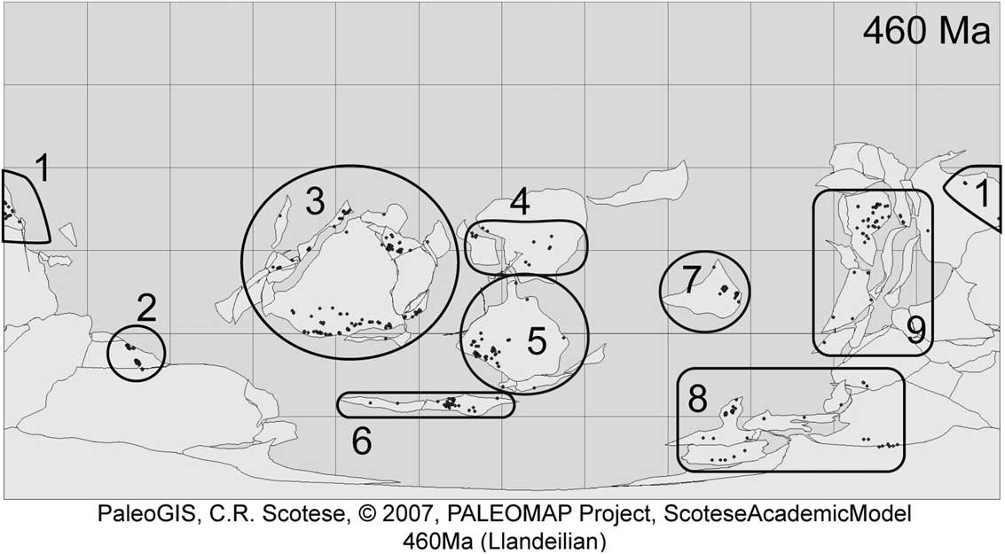
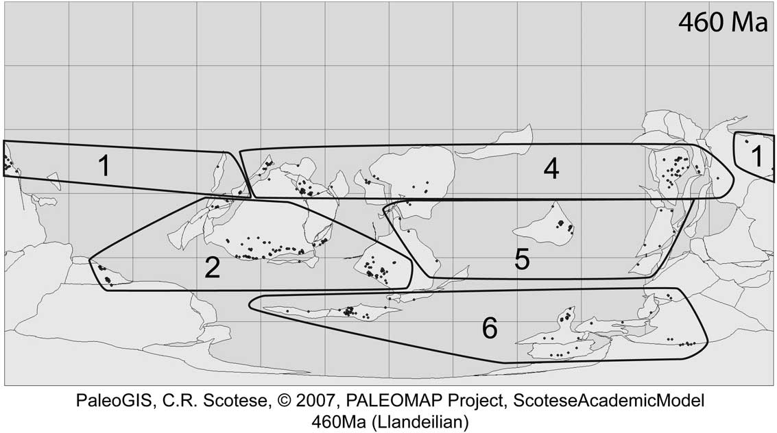
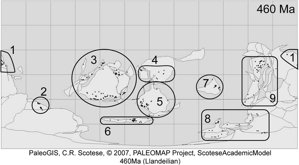
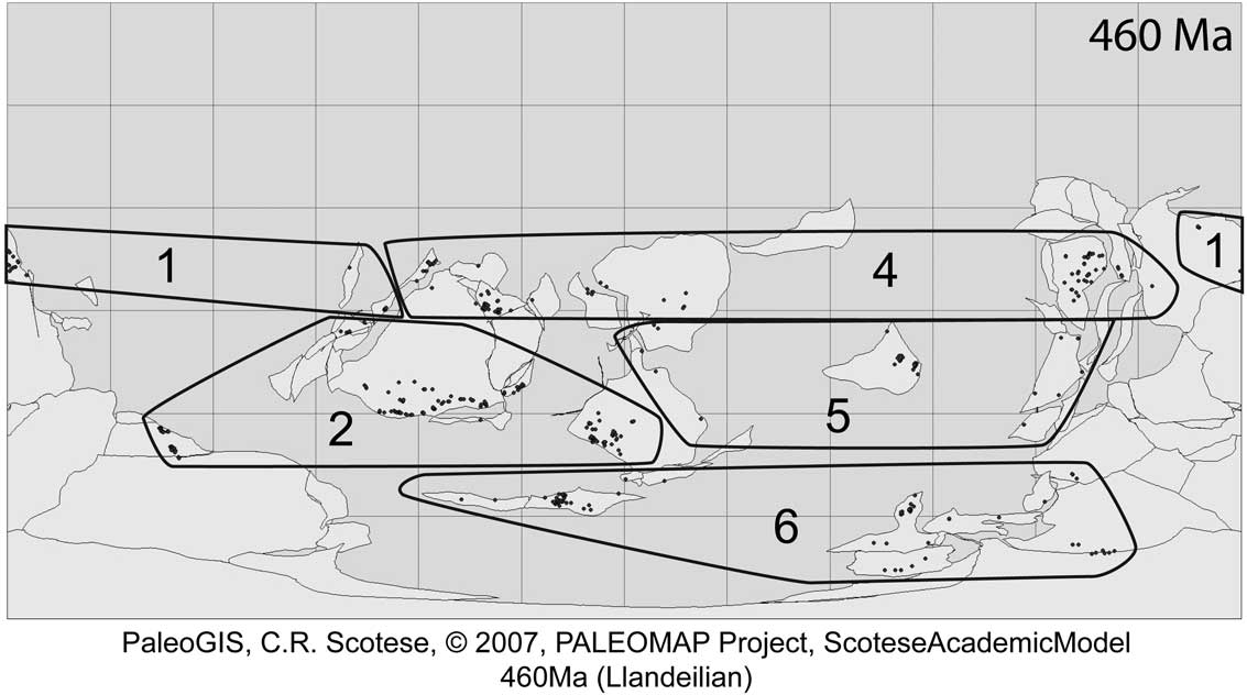
The number of geographical bins occupied has traditionally been used as a measure of geographic range in paleontological studies in recognition of the constraints on their spatial resolution. In this study geographical bins were defined in two different ways. First, we defined nine paleogeographic regions based on the spatial clustering of sections and paleocontinents (Fig. 2): northeast Gondwana, southeast Gondwana, Laurentia, Siberia, Baltica, Avalon, Kazakhstan, southwest Gondwana, and northwest Gondwana. In the second type of geographical bin, we placed sites into paleogyres (Fig. 3). Some modern plankton are distributed widely within gyres but confined to a particular gyre or set of gyres (Goetze 2011). Although graptolites likely had some control over their vertical position in the water column (Cooper et al. Reference Cooper, Rigby, Loydell and Bates2012), they probably were mainly carried passively in surface currents, so that their distribution might also have been determined by those currents. Thus, five to six oceanic gyres, depending on the time interval, were designated based on reconstructions from the literature (Wilde Reference Wilde1991; Le Hérissé et al. Reference Le Hérissé, Gourvennec and Wicander1997; Herrmann et al. Reference Herrmann, Haupt, Patzkowsky, Seidov and Slingerland2004). These gyres also include the large epicontinental seas covering much of the continents in the lower Paleozoic.
A Mercator paleogeographic reconstruction of the Ordovician world at 460 Myr from PaleoGIS, with the nine regions used in this study identified. Points on the map are occurrences of taxa examined in Boyle et al. (Reference Boyle, Sheets, Wu, Goldman, Melchin, Cooper, Sadler and Mitchell2014).
Map as in Fig. 2 with five of the six gyres used in this study identified. Gyre 3 is placed between gyres 2, 4, and 5 during some 10 Myr time intervals.
Sampling Measures
Because sampling (the sum of properties such as original abundance and collection effort, among other things) is known to affect calculated durations in CONOP (Sadler et al. Reference Sadler, Cooper and Melchin2009) and to covary with geographic range (Gaston Reference Gaston1994), it will also affect extinction risk. Furthermore, it is likely that the ecology of individual taxa will make some species more susceptible to the biases of the fossil record, thus altering the likelihood of sampling. For example, some graptolites are inferred to have predominantly inhabited deep water over the continental slope and rise settings (Cooper et al. Reference Cooper, Fortey and Lindholm1991), and so are less likely to be preserved in the fossil record than graptolites that inhabited continental basins or shelf environments. Consequently, we employed two different measures of sampling for each taxon. The first measure of sampling is the number of unique geographical locations at which a taxon is present. This measure combines sections whose locations were indistinguishable at the spatial resolution relevant here (i.e., sections being sampled on opposite sides of a riverbed). The second sampling measure is the number of individual sections at which a taxon is present. For this measure, we counted composite sections as a single occurrence rather than as four separate points, in contrast to the way we treated composites in the geographic-range calculations.
Another measure of taxon occurrence, the number of grid cells occupied, has become common in paleobiological studies (e.g., Finnegan et al. Reference Finnegan, Payne and Wang2008; Foote et al. Reference Foote, Crampton, Beau and Cooper2008; Harnik et al. Reference Harnik, Simpson and Payne2012) and appears to measure a compromise between geographic range and sampling (Kiessling and Aberhan Reference Kiessling and Aberhan2007). We employed a grid cell size of 5° because it was the minimum size that was still larger than the error associated with modern-day coordinates gathered from the literature. Because the cell sizes were based on degrees, the actual area covered by individual grids varies with latitude. However, most of the sections rest within 20° of the paleoequator and, thus, do not vary greatly in area.
Graptolite-Specific Factors
Geographic range and sampling affect the apparent extinction risk in all organisms, but the particular ecology of organisms makes some more vulnerable than others (Foden et al. Reference Foden, Butchart, Stuart, Vié, Akçakaya, Angulo, DeVantier, Gutsche, Turak, Cao, Donner, Katariya, Bernard, Holland, Hughes, O’Hanlon, Garnett, Şekercioğlu and Mace2013), and graptolites were no exception. The factors specific to graptolites considered as having a possible influence on extinction risk examined here include biofacies group, tolerance of shallow sites, clade, and two breakpoints in the time series where the extinction pattern in graptolites may have shifted: the base of the Katian and Rhuddanian stages (Cooper et al. Reference Cooper, Sadler, Munnecke and Crampton2014).
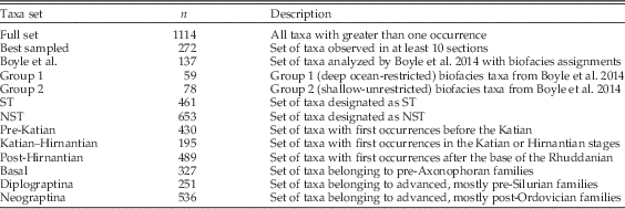
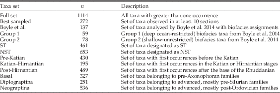
The most well-established influence on graptolite extinction among the above factors is biofacies group. Biofacies affiliations are currently recognized only for Ordovician taxa, and Cooper and Sadler (Reference Cooper and Sadler2010) categorized 153 taxa into either group 1 or 2. Group 3 taxa were not examined, because they are usually poorly represented in the fossil record. Here, we employ the same subset of 137 of those taxa to conduct a set of further detailed analyses. This set (which omits 16 poorly sampled species and is the same subset employed by Boyle et al. Reference Boyle, Sheets, Wu, Goldman, Melchin, Cooper, Sadler and Mitchell2014) includes 59 group 1 taxa and 78 group 2 taxa. In an attempt to approximate the biofacies affiliation of a greater number of taxa, we classified each of the 512 stratigraphic sections as either shallow (continental shelf deposits above storm wave base) or deep (deposits of epicratonic basins, continental slopes, or abyssal sediments). Following the ecological interpretation of biofacies groups as both a lateral and vertical segregation of taxa (Cooper et al. Reference Cooper, Fortey and Lindholm1991; Cooper and Sadler Reference Cooper and Sadler2010), any taxa that occur in shallow deposits are likely to belong to group 2 or to group 3 (the shelf-endemic group). Therefore, we put all taxa that occur in at least one shallow site into a shallow-tolerant (ST) biofacies group (n=461), and the remaining taxa (n=653) were assigned to a non–shallow tolerant (NST) biofacies group.
Clade membership is known to influence extinction risk (Hoffman and Kitchell Reference Hoffman and Kitchell1984; Stanley et al. Reference Stanley, Wetmore and Kennett1988; Mitchell Reference Mitchell1990; Jablonski and Raup Reference Jablonski and Raup1995; Jeffery Reference Jeffery2001; Chen et al. Reference Chen, Melchin, Sheets, Mitchell and Jun-Xuan2005; Foote et al. Reference Foote, Crampton, Beau and Cooper2008; Bapst et al. Reference Bapst, Bullock, Melchin, Sheets and Mitchell2012). To assess clade membership as a possible correlate of extinction risk, we employed recent phylogenetic analyses (Fortey and Cooper Reference Fortey and Cooper1986; Mitchell et al. Reference Mitchell, Sheets, Belscher, Finney, Holmden, LaPorte, Melchin and Patterson2007; Maletz et al. Reference Maletz, Carlucci and Mitchell2009) to assign taxa in this study to 16 family-level clades (see also Sadler et al. [Reference Sadler, Cooper and Melchin2011], who employed the same taxon set to analyze clade diversity patterns). The influence of clade on extinction risk in graptolites is evident from the selective extinction of most branches of the graptolite tree during the LOME (Melchin and Mitchell Reference Melchin and Mitchell1991; Chen et al. Reference Chen, Melchin, Sheets, Mitchell and Jun-Xuan2005; Bapst et al. Reference Bapst, Bullock, Melchin, Sheets and Mitchell2012). The LOME appears to have marked a change in the extinction regime even for clades that survived the event (Chen et al. Reference Chen, Melchin, Sheets, Mitchell and Jun-Xuan2005; Bapst et al. Reference Bapst, Bullock, Melchin, Sheets and Mitchell2012). To test this hypothesis, we included an age factor in the analyses by grouping taxa as Ordovician versus post-Hirnantian based on the age of their FAD relative to the base of the Rhuddanian, which is marked by the first appearance of Akidograptus ascensus at the Silurian global stratotype section and point (GSSP), Dob’s Linn, Scotland (Rong et al. Reference Rong, Melchin, Williams, Koren and Verniers2008; Melchin et al. Reference Melchin, Sadler, Cramer, Cooper, Gradstein and Hammer2012). Cooper et al. (Reference Cooper, Sadler, Munnecke and Crampton2014), on the other hand, hypothesized that the extinction regime shift occurred earlier in graptolite history, in the early Katian, based on similarities between increased species turnover rates and volatility of the isotopic composition of the carbonate carbon reservoir. Consequently, we also subdivided the time series at the base of Katian, which is marked by the first occurrence of Diplacanthograptus caudatus at the Katian GSSP, Black Knob Ridge, Oklahoma (Goldman et al. Reference Goldman, Leslie, Nõlvak, Young, Bergström and Huff2007; Cooper and Sadler Reference Cooper and Sadler2012). These two break points allowed taxa to be grouped into three cohorts: pre-Katian, Katian–Hirnantian, and post-Hirnantian.
Data Analysis
Previous statistical analyses of graptolite extinction risk have been limited to Ordovician taxa with biofacies group assignments (Cooper and Sadler Reference Cooper and Sadler2010; Boyle et al. Reference Boyle, Sheets, Wu, Goldman, Melchin, Cooper, Sadler and Mitchell2014), but here we analyze 1114 taxa of all ages, using several different types of subdivisions of the data to examine a range of questions. To examine the factors associated most strongly with extinction risk in different sets of taxa (i.e., different clades or age cohorts) and to limit sampling biases, we split the full set of taxa into 12 different subsets that we analyzed individually in addition to the full set (Table 2). Because most families included too few species to permit rigorous analysis of individual clades, we combined them into three higher-order clades for analysis: a “basal” paraclade comprising essentially the entire Graptoloida, excluding only the Axonophora (Maletz et al. Reference Maletz, Carlucci and Mitchell2009), with the remaining Axonophora divided into their two major sister clades, the Diplograptina and the Neograptina (Štorch et al. Reference Štorch, Mitchell, Finney and Melchin2011; Melchin et al. Reference Melchin, Mitchell, Naczk-Cameron, Fan and Loxton2011). A small number of the stem axonophorans were included with the Diplograptina for the purposes of this analysis. Thus, our Diplograptina+stem Axonophora is equivalent to the paraphyletic Diplograptina as used by Maletz (Reference Maletz2014). The Neograptina is a monophyletic clade that contains the monograptids (sensu Melchin et al. Reference Melchin, Mitchell, Naczk-Cameron, Fan and Loxton2011; non Maletz Reference Maletz2014).
Sample size and description of each of the taxon subsets analyzed.
Hypothesis Testing, General Linear Models (GLMs), and Partial Least-Squares Regression (PLSR)
In this study, we tested for differences between the species’ durations, geographic ranges, age cohorts, and sampling values of 13 different taxon sets and subsets. Because variance in these properties were not normally distributed, we used Wilcoxon tests to examine these contrasts and adjusted significance levels via false discovery rate (Curran-Everett, Reference Curran-Everett2000) to control family-wise error rate in the large number of comparisons within each set of taxa. The R code used to run the analyses below is located in the Supplementary Material (Supporting Information 1).
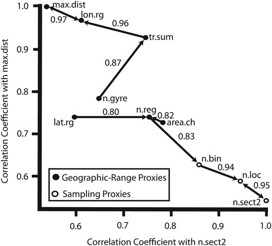
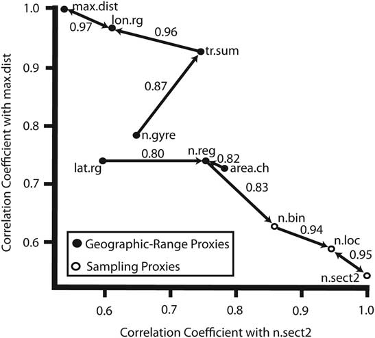
To examine the effects of the measured variables on extinction risk, we constructed a series of GLMs for single factors and for combinations of factors. These models are a combination of linear regression and analysis of variance (ANOVA) analyses that can handle multiple factors (continuous and categorical) and the interactions between factors. From each GLM, the proportions of the total variance in graptolite durations explained was extracted and compared via ANOVA. Because several of the independent variables were intended to measure the same property (geographic range or sampling), many of these were strongly correlated with one another (Fig. 4). This correlation complicates the interpretation of differences in variance explained by different measures of geographic range or complex models.
Plot showing the correlation structure between sampling and geographic-range measures used in the analyses. Arrows point to the factor with the highest correlation coefficient, which is labeled along the arrow. n.sect2 is the number of sites occupied counting composites as a single occurrence; n.loc is the number of distinct geographic locations occupied; n.reg is the number of paleoregions occupied; n.gyre is the number of paleogyres occupied; lat.rg is the latitudinal range in degrees; max.dist is the maximum pairwise distance; tr.sum is the summation of a minimum spanning tree of occurrences; n.bin is the number of 5°×5° cells occupied; lon.rg is the longitudinal range in degrees; and area.ch is the convex-hull area occupied.
To account for the covariance among the variables and to make interpretation of complex models more feasible, we reduced the dimensionality of the predictor variables in the data set by PLSR analysis using the pls package (Mevik and Wehrens Reference Mevik and Wehrens2007) in the R programming environment before conducting the GLM analysis step. The plsr() function within the pls package was used for each data set, with the number of axes set to the number of independent variables (10–12) and all other parameters left at the default settings. PLSR analysis uses the covariance structure among the original variables to construct a smaller set of independent axes, or synthetic variables, that capture the shared information content of the originals. The first of these axes has the strongest covariance, the second axis has the next greatest covariance, and so forth. Because of this, the variance explained by each axis is not necessarily in the same rank order, so that the second axis might explain less variance than the third PLSR axis while still capturing a larger fraction of the total covariance. Because PLSR is sensitive to the relative magnitudes of the variance in the data, we standardized the data by z-transformation prior to PLSR analysis. Binary variables (biofacies association and shallow tolerance) were dummy coded with ones and zeros and then z-transformed. Categorical data with more than two states (clade, age cohort) could not be included in the PLSR analysis, because the differences in value states would be interpreted incorrectly as metrical distance by the PLSR analysis. The PLSR analysis provided a score for each taxon on each independent axis, and we employed these axis scores as derived variables in the GLM analyses, in which they were treated in the same way as the untransformed data.
Model Ranking and Significance Testing
To rank each GLM relative to each of the others, we used Akaike information criterion (AIC) scores (Akaike Reference Akaike1974). AIC scores provide a means to measure the relative strength of a set of models based on their likelihood while at the same time penalizing models with larger numbers of parameters. However, AIC score ranking may favor models that are overfit, particularly at small sample size (Seghouane Reference Seghouane2011); we therefore employed permutation methods to test whether each GLM model was able to explain a greater percentage of the variance in durations than would be expected by chance. For each model, species durations were randomly shuffled among the graptolite taxa 1000 times while preserving the covariance structure of the independent variables. A GLM was fit to each of the 1000 data permutations, followed by an ANOVA analysis to determine the percent variance explained in each permuted set for all models examined. The distribution of the variances in durations explained by each of the permuted models was then compared with the actual variance explained. The proportions of total permutations that possessed a variance in durations less than the variance in durations explained for the real data was taken as the p-value, with an alpha of 0.05. For the PLSR composite axis variables, sequential axes were permuted by holding the duration and previous axes constant and shuffling only the scores corresponding to the axis of interest, which allowed the explanatory power of the previous axes to be controlled, that is, taken into account, as we evaluated whether each successive axis added a greater percent variance in durations than expected by random permutations. After all permutation tests, a false discovery rate was used to account for family-wise error rate among permutation tests with the highest-ranked models (ranked first by p-value and then by AIC value in the case of ties) having the most stringent significance thresholds.
Results
Extinction Risk in Graptolites
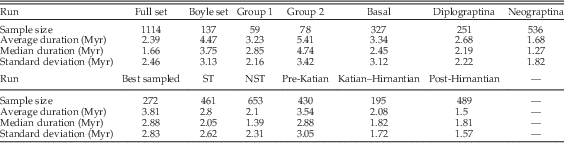
The median and average durations of each set of taxa were calculated (Table 3) and Wilcoxon tests showed significant differences in all complementary comparisons except between the basal clades and the Diplograptina (Table 4). Group 2 taxa and ST taxa had significantly greater durations than group 1 and NST taxa, respectively. Among the three higher-order clades, the basal paraclade taxa tend to have greater durations than the Diplograptina, and both tend to have greater durations than members of the Neograptina. Taxa grouped by FAD age (taxon age cohorts) produced a set of duration contrasts that corresponded closely with those of the major clades: pre-Katian taxa (dominantly basal paraclade taxa but also with a significant number of Diplograptina) tend to have the greatest durations, whereas the post-Hirnantian taxa (which are entirely Neograptina) have the shortest average durations and the Katian–Hirnantian set (mainly Diplograptina with a minor component of Neograptina) had intermediate durations.
Sample sizes, average and median durations, and standard deviations of durations for each run.

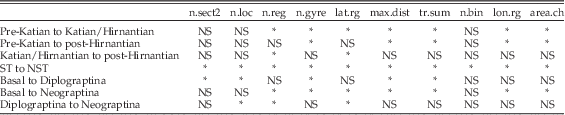
Wilcoxon tests for significant differences in geographic range and sampling measures between taxon subsets after false discovery rate correction. NS, p≥0.05; *, p<0.05. See Fig. 4 for explanations of the column headings.

Wilcoxon tests for significant differences in measures of geographic range and sampling between taxon subsets produced a more mixed set of outcomes (Table 4), possibly as a result of smaller sample sizes, which reduced test power. For both the biofacies groups and the ST sets, one taxon set, group 2 and ST taxa, respectively, had values of geographic range and sampling that were, on average, twice as large as their counterparts. In the higher-order clade set, taxa of the basal paraclade have the greatest geographic range, on average. The Diplograptina tend to be the most well sampled, but this difference is not significant. The Neograptina have, on average, the largest values of latitudinal range and number of regions occupied. Once again, the taxon age cohorts show patterns similar to those of the clades. The pre-Katian taxa tend to have the largest geographic range, and post-Hirnantian taxa have the greatest latitudinal range and number of regions occupied, on average.
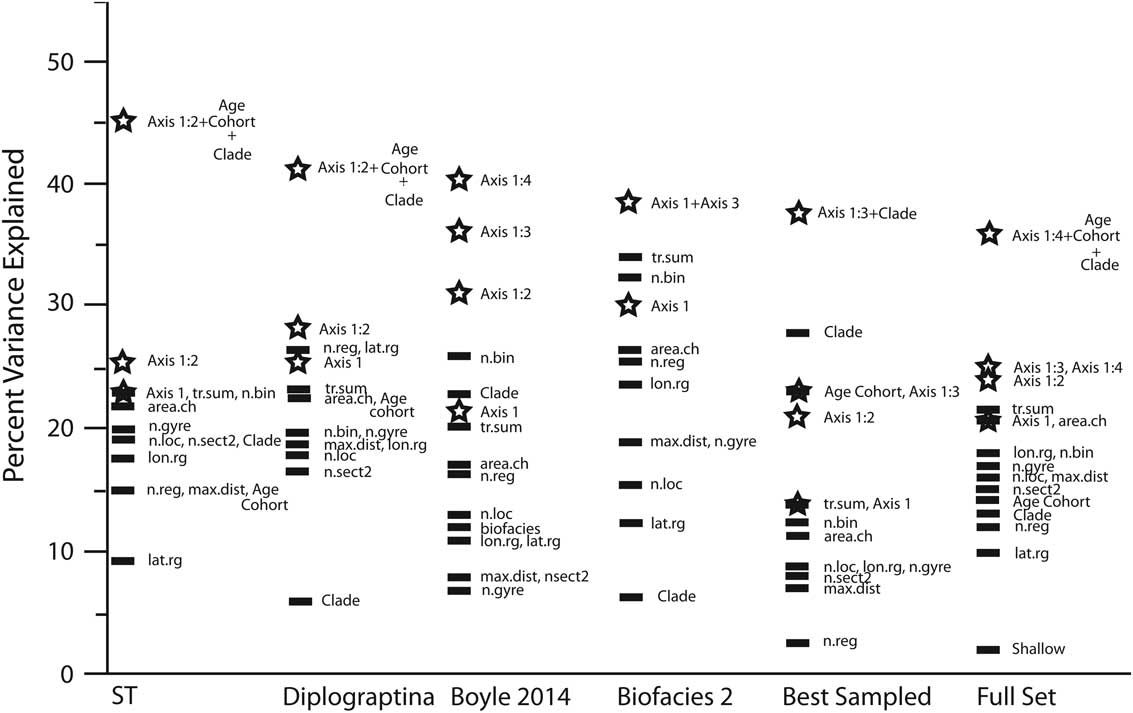
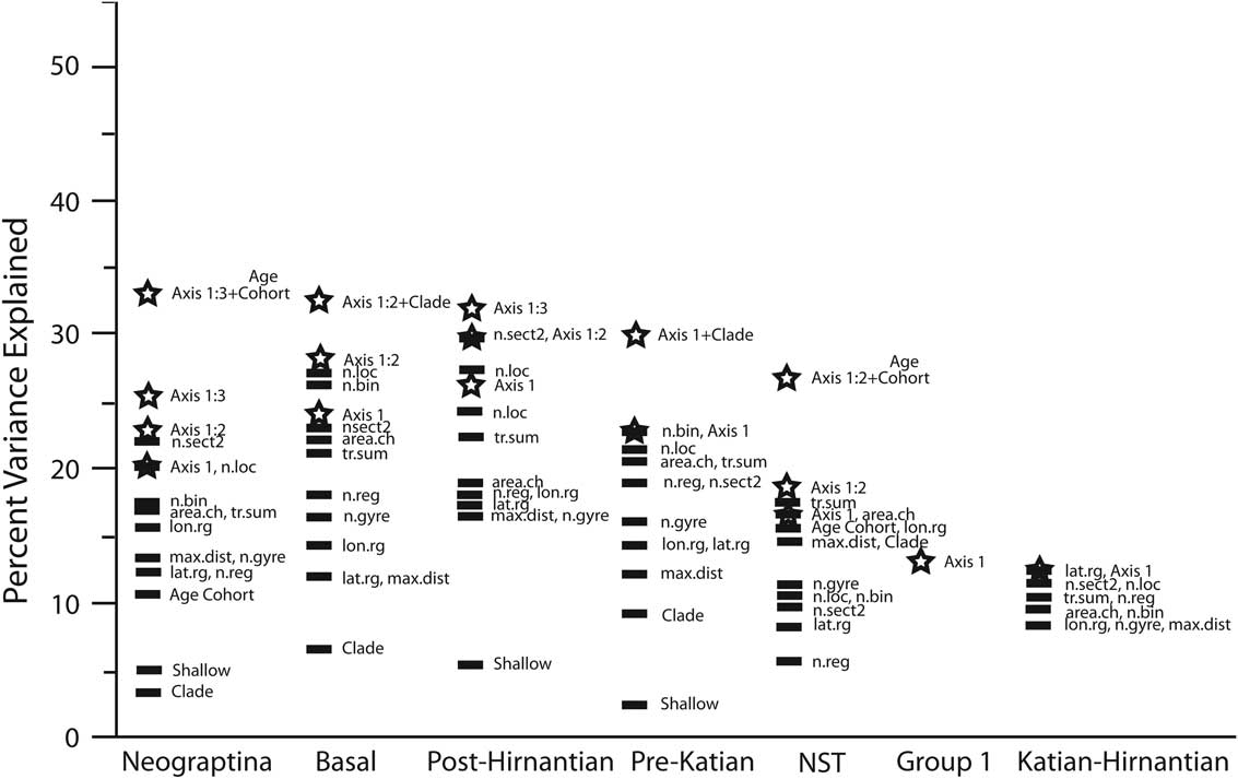
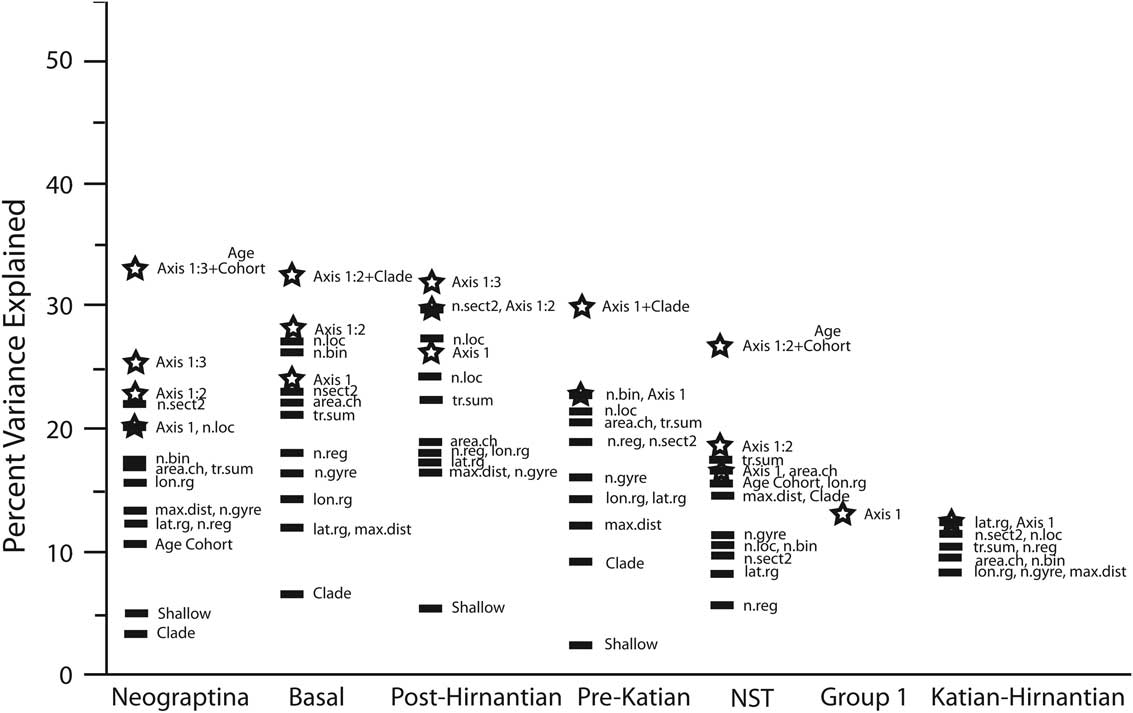
The significant variance in durations explained by single untransformed factors (excluding the composite variables derived from PLSR) varied among sets from 2% to 34% (Figs. 5, 6). Among the single factors, the number of 5°×5° cells, summation of minimum spanning tree, and convex-hull area have consistently high explanatory power. On the other hand, maximum pairwise distance, latitudinal range, and shallow tolerance were consistently the lowest-scoring factors.
Results from analysis of six different taxon sets, showing significant percentages of variance explained by single factors, PLSR axes, or GLM models of composite PLSR axes plus age cohorts and clade. Abbreviations as in Fig. 4. Stars represent composite PLSR axes. Axis 1:n represents the summed variance in durations explained of the first to nth composite PLSR axes.
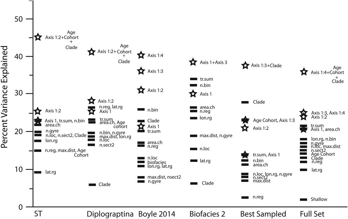
Results from analysis of seven different taxon sets, showing significant percentages of variance explained in durations by single factors, PLSR axes, or GLM models of composite PLSR axes plus age cohorts and clade. Abbreviations as in Figure 4. Stars represent composite axes. Axis 1:n represents the summed variance explained of the first to nth composite PLSR axes.
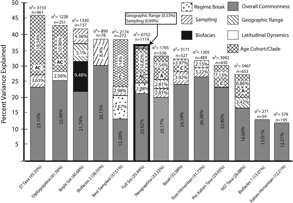
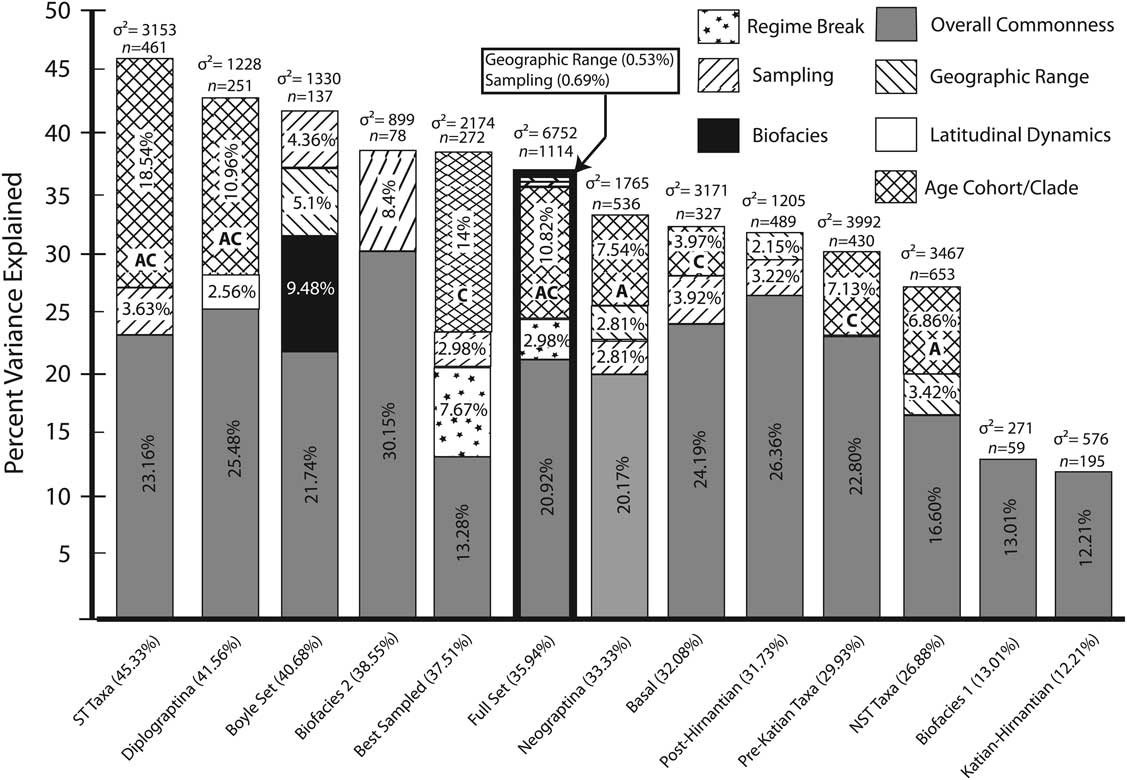
In the PLSR analysis, after permutation tests and controlling for family-wise error rate, no more than four PLSR composite axes were found to be significant for any of the taxon sets (Fig. 7). In most cases there were two or three significant composite axes. The total significant variance explained in durations by PLSR axes ranges from 12% to 41% of the total variance in any given set. Clade and age cohort, because they could not be included in the PLSR analysis, were added onto the significant PLSR axes. Clade alone was found to add significant variance in three taxon sets, age cohort alone added significant variance in two taxon sets, and in three sets both age cohort and clade added additional variance. Where significant, clade and age cohort factors explained between 4% and 19% additional variance in durations when added to the PLSR composite axes. In all taxon sets, with the exception of the Katian–Hirnantian set, those models that had highest variance explained were also those most strongly favored by AIC. In the Katian–Hirnantian set, latitudinal range is favored by a very small margin over the first PLSR composite axis by both AIC (744.4 vs. 745.1) and percent variance explained (12.61% vs. 12.21%).
Stacked histogram showing the percent variance in durations explained by significant PLSR composite axes, age cohort, and clade for each of the 13 taxon sets. Numbers below each bar are the significant percent variance explained by the best models, while the numbers above each bar represent sample size and total variance of durations. “A” and “C” in the columns indicate (respectively) whether age cohort or clade alone explains the indicated variance in durations. Bold outline highlights the full set of 1114 taxa.
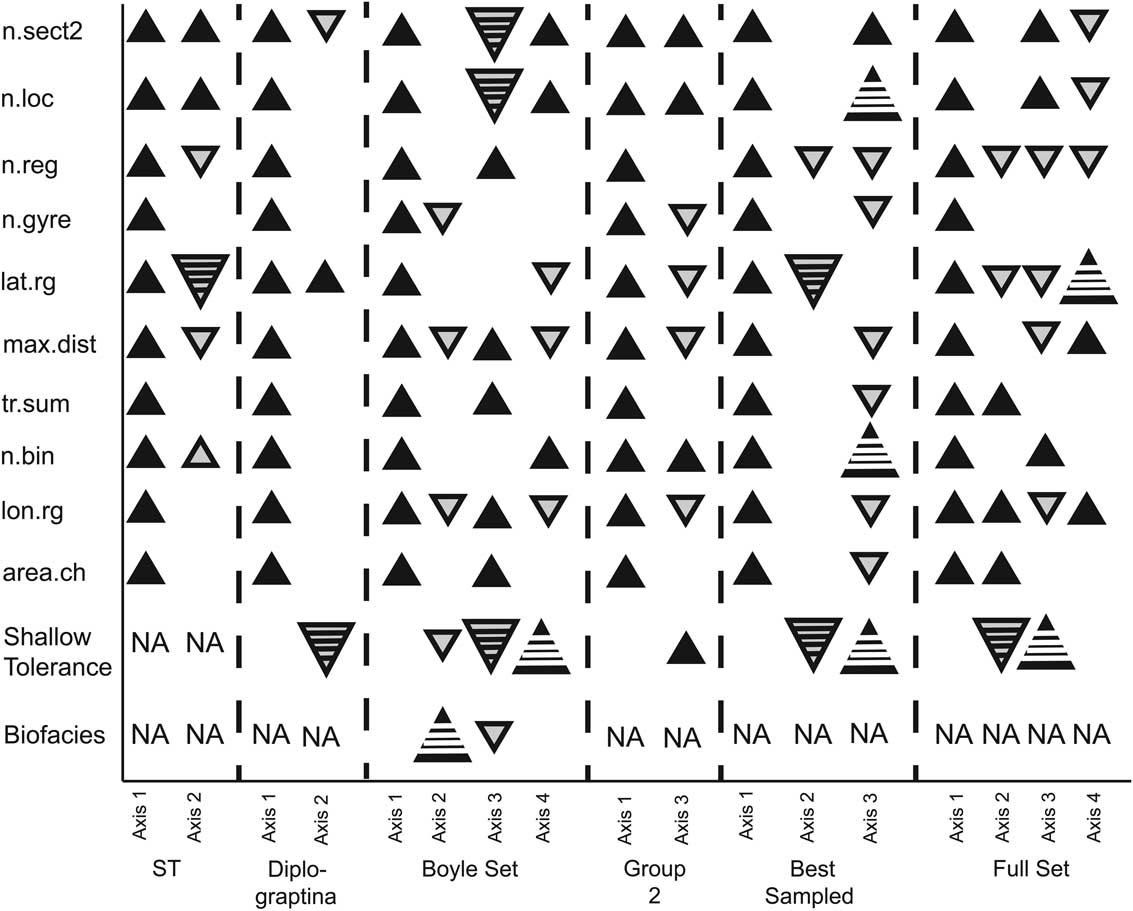
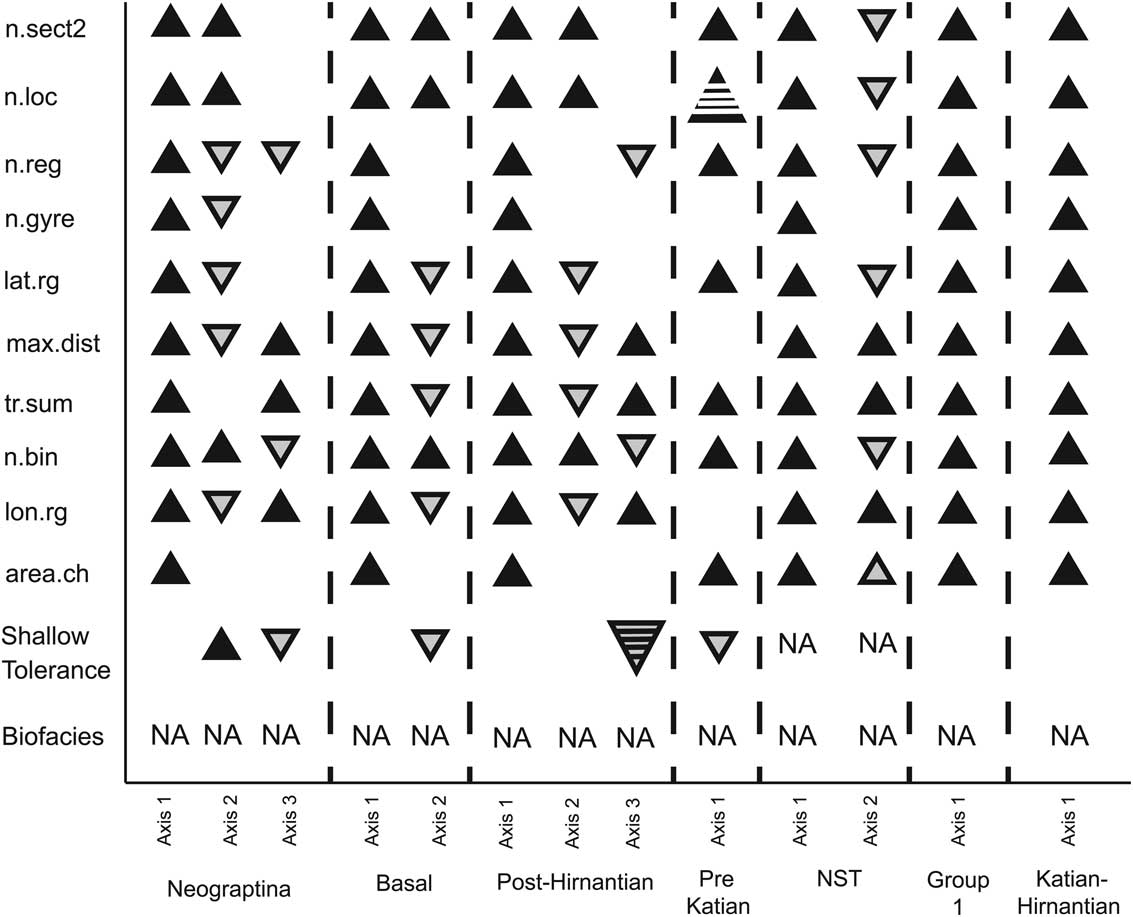
In all sets the first axis was a near-equal weighting of all measures of geographic range and sampling (Figs. 8, 9). This set of covariates appears to capture the effect on extinction risk of overall commonness through the correlated behavior between the number of observations and geographic range. This first axis explained 12–30% of the total variance in durations, and accounts for the largest proportion of the variance explained by PLSR axes for all GLM models. Further axes were more variable between sets of taxa (see Supporting Information 2 for loading values for each PLSR composite axis for each taxon set). In the case of the full taxon and best-sampled taxa sets, the second composite axis is dominated by a strong negative weighting on latitudinal range and shallow tolerance, which we interpret as reflecting the difference between the Neograptina (regime break in Fig. 7) and the remaining taxa. This is based on the observation that the Neograptina have significantly greater latitudinal ranges and an underrepresentation of ST taxa despite having statistically shorter durations than the other clades, possibly as a result of increased shale deposition during the latest Ordovician and early Silurian (Melchin et al. Reference Melchin, Mitchell, Holmden and Štorch2013). This interpretation is consistent with taxa in Neograptina having negative scores on this axis. In the case of the Diplograptina set, the second axis is unique. It exhibits a moderate positive weighting by latitudinal range and a very strong negative weighting of shallow tolerance (latitudinal dynamics in Fig. 7). This weighting is interpreted as a difference in the rate of decrease in extinction risk with increasing latitudinal range between the two depth-related taxon sets. The NST Diplograptina have a slower rate of decrease in extinction risk with increasing latitudinal range than do the ST taxa.
PLSR composite axis-loading values for six of the 13 taxon sets. Upward-pointing black triangles represent positive loading (small solid: 0.2 to 0.6; large striped: >0.6). Downward-pointing gray triangles represent negative loading (small solid: [−0.2] to [−0.6]; large striped: <[−0.6]). Blank areas represent loading of 0±0.2. NA represents factors that were not applicable to the subset.
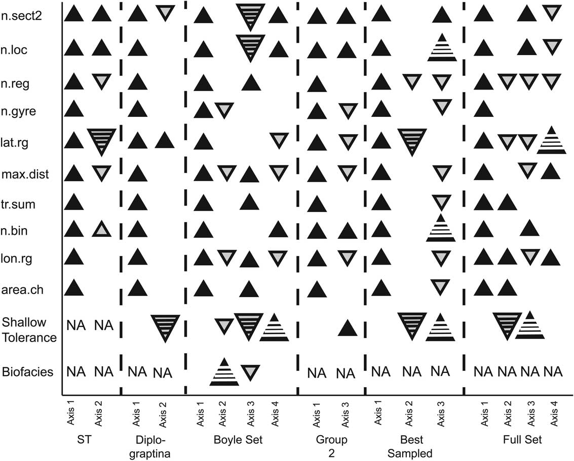
PLSR composite axis loadings for 7 of the 13 taxon sets. Symbols as in Fig. 8.
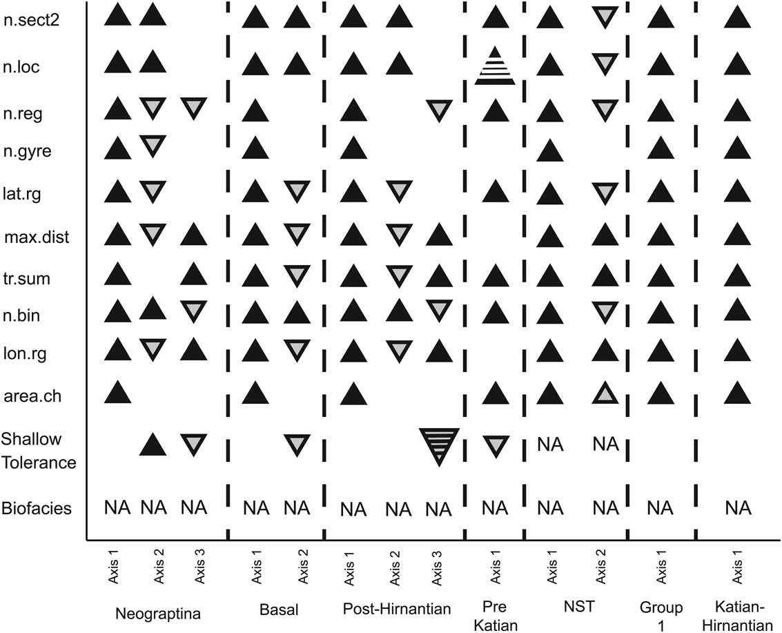
The effect of extensive sampling despite a small geographic range (indicated by positive weighting on number of localities, number of sections, and number of 5°×5° cells occupied, coupled with negative weighting on geographic range measures) is significant in eight sets of taxa (ST, Neograptina, post-Hirnantian, Boyle et al., biofacies 2, best sampled, full set, and basal). The reverse, a positive weighting on geographic-range measures and negative weighting on sampling measures, represents the impact of a large geographic range despite a low level of sampling. This axis was found in five sets, but the geographic-range measures that are positively weighted differ among them: latitudinal range for the best-sampled set, number of gyres and latitudinal range for ST taxa, latitudinal range and longitudinal range for the full set, and maximum pairwise distance and longitudinal range for the post-Hirnantian and Boyle et al. sets. The variance in durations explained by the effects of either dense sampling or large geographic range despite sparse sampling are relatively minor components. They explain only 0.5–8% additional variance. As reported in Boyle et al. (Reference Boyle, Sheets, Wu, Goldman, Melchin, Cooper, Sadler and Mitchell2014), the second axis of the PLSR analysis of the taxa with biofacies group assignments is dominated by positive weighting on biofacies group and explains 9.48% of the total variance in durations. This factor is unique to this analysis, as biofacies group assignments are not available for most graptolite taxa, and in addition, it is not clear whether this division is applicable to post-Hirnantian taxa.
Discussion
Despite their extensive use in early Paleozoic biostratigraphy, controls on extinction risk among graptolites have only recently been analyzed quantitatively. Cooper and Sadler (Reference Cooper and Sadler2010) examined biofacies groups, geographic range (coded as two states: endemic or pandemic), and occupancy ratio (measured as the proportion of sites within a species’ duration at which it has been recovered) as possible predictors of extinction risk in 153 Ordovician graptolites. They found that species restricted to the deep-water deposits (group 1) had a significantly greater extinction risk than the species that were not limited to deep-water deposits (group 2) and that biofacies affiliation alone accounted for most of this difference in extinction risk. Geographic range and occupancy ratio contributed little additional explanatory power on their own. The durations of graptolites that Cooper and Sadler used have been updated with additional sections (Cooper et al. Reference Cooper, Sadler, Munnecke and Crampton2014) and their extinction risk reevaluated with additional measures of sampling and geographic range (Boyle et al. Reference Boyle, Sheets, Wu, Goldman, Melchin, Cooper, Sadler and Mitchell2014). Boyle et al. (Reference Boyle, Sheets, Wu, Goldman, Melchin, Cooper, Sadler and Mitchell2014) found that biofacies grouping was the second-strongest factor associated with extinction risk after overall commonness (the correlated effects of sampling and geographic range). Expanding the analysis to all planktic graptolites reveals that clade affiliation and age cohort are also significant risk factors. Furthermore, the new analyses reveal a complex pattern of changing extinction risk that depends not only on general species properties, such as geographic range, but also on ecological factors (e.g., biofacies groups) and abiotic events (e.g., the LOME) that reshaped the group’s evolutionary regime.
Geographic Range and Sampling
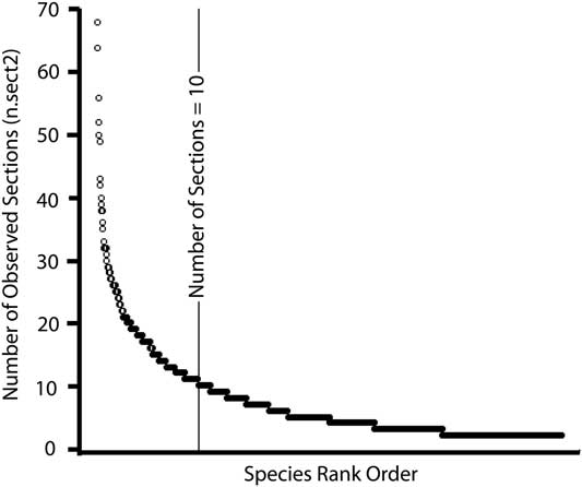
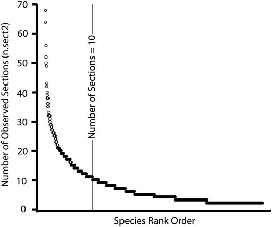
In all sets of analyzed taxa, the dominant predictor of extinction risk was the correlated effects of geographic range and sampling that we refer to as overall commonness. Taxa seen in a greater number of sites and with wider geographic ranges had a lower extinction risk. To the extent that our sampling measures are a true proxy for sampling completeness, the result that overall commonness is the strongest predictor of extinction risk suggests that despite the intense sampling of graptolites as a group, the record for individual species is still fragmentary. In fact, the majority of species are seen in fewer than 10 sections (Fig. 10), and the distribution of observations is strongly skewed. When we restrict our analysis to a set of 272 taxa observed in at least 10 sections (“best sampled”), the resulting model has the third-weakest overall commonness factor. Instead, effects having to do with clade and cohort age were the dominant factors. Overall commonness in the best-sampled set explained only ~13% of the variance in taxon duration, approximately half as much as the average among the other sets of taxa. This suggests that half of the effect on extinction risk commonly attributed to geographic range may be a product of sampling effects, which is supported by the amount of variance explained by individual factors. The maximum pairwise distance, which has the lowest correlation with sampling measures (Fig. 4), explains approximately half as much variance as the first composite axis, overall commonness. Studies that have sought to distinguish between the effects of geographic range and sampling on extinction risk have most often suggested that the effects of geographic range are dominant over sampling (Payne and Finnegan Reference Payne and Finnegan2007; Powell Reference Powell2007; Harnik Reference Harnik2011; Finnegan et al. Reference Finnegan, Heim, Peters and Fischer2012). However, most focused explicitly on the best-sampled taxa, typically above species level, to maximize the number of observed occurrences and minimize the effects of sampling (Powell Reference Powell2007; Harnik Reference Harnik2011).
All 1114 taxa ordered by the natural log of the number of sites observed at (n.sect2).
Individual contributions from sampling and geographic range appear in nine of the taxon sets and explain a much smaller, although still significant, proportion of the total variation. Sampling, despite small geographic range, was seen in nine sets (Fig. 7) but without much apparent pattern. The impact of sampling in those sets is reflected in single-factor models in which number of localities, number of sections, and number of 5°×5° cells occupied are higher in rank for the basal paraclade, Neograptina, and post-Hirnantian sets than is the case for the other sets (Figs. 5, 6), suggesting these groups are poorly sampled. The reasons for this, particularly among the post-Hirnantian taxa for which graptolites are used extensively in biostratigraphy, may be because of the way graptolites are typically collected.
The majority of studies involving graptolites are interested in their use as biostratigraphic markers rather than paleoecological or evolutionary questions about the graptolites themselves. Consequently, investigators focus on collecting specimens that are well preserved and distinctive, rather than bulk samples that might reveal additional species. Focus is also given to locating the first and last occurrence of a species within a sequence to delineate biozone boundaries, with less emphasis given to documenting the persistence or abundance of a species between its first and last occurrences. These types of collection biases, typical of the graptolite occurrence data used to calculate durations, were not modeled or controlled for in this study and would likely explain additional variance between taxa. Particularly between those taxa considered to be stratigraphically important and all others. Differences between taxa that are numerically abundant versus rare might also be expected to correlate with extinction risk, as rare species are more likely to have their ranges within sections truncated and less likely to be collected in the field because the chances of finding well-preserved individuals are lower. In benthic taxa the effect of abundance on extinction risk has been found to be weak or not significant after controlling for geographic range (Harnik Reference Harnik2011; Harnik et al. Reference Harnik, Simpson and Payne2012; but see Simpson and Harnik [Reference Simpson and Harnik2009] for an exception). However, work on planktonic foraminifera found support for higher extinction risk in clades with low abundance (Stanley et al. Reference Stanley, Wetmore and Kennett1988).
Where it can be separated from sampling, the relatively small contribution of large geographic range to extinction risk in graptolites is unusual. On its own, geographic range accounted for less than 3% of the total variance in durations and was only a significant factor in five sets (Boyle, full set, Neograptina, post-Hirnantian, and NST). Large geographic range is typically highly predictive of reduced extinction risk across other clades (Jablonski Reference Jablonski2005 and references therein). The small effect in our analyses may reflect the impact of the strong correlation of variables in this study, where the explanatory power of large geographic range is tied up in the composite axis that we interpreted as overall commonness. However, there also is reason to believe that the contribution of geographic range to extinction risk in graptolites may genuinely have been lower than that in other groups (i.e., benthic invertebrates) because most planktic graptoloids were comparatively widespread. For example, Foote and Miller (Reference Foote and Miller2013), using great circle distances, reported that 98% of the benthic invertebrates they examined had a maximum range size of less than or equal to 15,442 km, whereas only 69% of the 1114 taxa examined here fall into this category using the maximum pairwise distance. In the best-sampled set only 35% of the taxa have geographic ranges smaller than 15,442 km. Graptolites are, therefore, generally much more widespread than benthic invertebrates. Graptolite geographic ranges are particularly large when one considers that the continents were confined almost exclusively to the Southern Hemisphere for much of the lower Paleozoic (Torsvik and Cocks Reference Torsvik and Cocks2013), which limits the maximum observed geographic range to essentially half the Earth’s surface. Given that most graptolite populations inhabited shelf-edge environs (Finney and Berry Reference Finney and Berry1997; Cooper et al. Reference Cooper, Rigby, Loydell and Bates2012), this observational limit may also closely approximate their original life occurrence limitations as well.
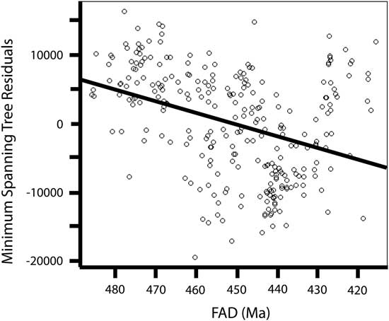
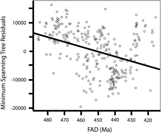
Thus, because the benefits of a large geographic range to decreasing extinction risk are logarithmic rather than linear (the largest effects arise from modest increases in small ranges; Foote and Miller Reference Foote and Miller2013: Fig. 3a), the influence of geographic range should be small compared with other factors given the large geographic range of most species. Perhaps not surprisingly, three of the analyses that exhibited strong effect of an individual geographic- range component (the post-Hirnantian, Neograptina, and NST sets) are also the sets that had the smallest average geographic ranges. The present data exhibit a significant trend toward smaller geographic-range size over time (Fig. 11), which may have been driven by the amalgamation of continents over the course of the early Paleozoic. The reduced average size of geographic ranges in later taxa, because of the logarithmic relationship between geographic range and extinction risk (Foote and Miller Reference Foote and Miller2013), increases the slope of the relationship and, thus, its observed strength. It is interesting to note that this interval of falling geographic-range size is also the same interval over which graptolite species diversity exhibits an unsteady but overall decline toward the ultimate extinction of the clade in the Early Devonian (see, for instance, Sadler et al. Reference Sadler, Cooper and Melchin2011).
Plot of the residuals from a correlation of the summation of a minimum spanning tree distance with number of observed locations versus time for the full set of 1114 taxa showing a significant negative trend (p<0.001).
It also possible that the relatively weak predictive ability of geographic range is attributable to the ecology of graptolites. Geographic range is expected to decrease extinction risk by decreasing the chance that single events will wipe out the entire population (Jablonski Reference Jablonski2005; Foote et al. Reference Foote, Crampton, Beau and Cooper2008). However, this expectation does not take into account the impact of geographic range on the likelihood of pseudoextinction, the apparent extinction of species when it evolves to a new form. The impact of geographic range on pseudoextinction depends on the distribution of a taxon within its geographic range. A relatively continuous distribution is likely to depress pseudoextinction by preventing isolation of populations (Lester and Ruttenberg Reference Lester and Ruttenburg2005), while a patchy or ephemeral distribution may actually encourage the formation of isolates and new species (Levin and Wilson Reference Levin and Wilson1976; Stanley Reference Stanley1979). A group with a high dispersal ability may achieve a large geographic range, especially when calculated using the union of all occurrences, and may have a high extinction risk due to the patchy nature of their distribution leading to pseudoextinction.
When geographic range-measures were examined as single-factor predictors of extinction risk, summation of a minimum spanning tree was often the highest-ranked model (Figs. 5, 6). This measure has not commonly been used as a measure of geographic range but has several advantages over other measures such as the maximum pairwise distance. Because this measure minimizes the distance between a series of points, it represents the minimum distance a taxon must have crossed, and this is particularly useful in this data set in which no corrections were made to avoid including uninhabitable areas (e.g., land). The data required to calculate summation of a minimum spanning tree is minimal, easily calculated in R, and can approximate complex geographic-range shapes. In contrast, the maximum pairwise distance is a poor predictor of extinction risk overall, probably because it is unable to account for complex geographic-range boundaries. Maximum pairwise distance ignores any range perpendicular to the bearing measured and is likely to greatly underestimate the true range of a species, particularly those that are wide-ranging or that have nearly circular or spatially complex distributions. It is also worth noting that some of the weakness of the maximum pairwise distance as a predictor of extinction risk might be due to the fact that we did not account for the possibility that a taxon might stretch around more than half the Earth’s circumference. This is likely to underestimate a taxon’s actual maximum pairwise distance and might weaken the relationship between this measure and extinction risk. However, when we tested this by analyzing the explanatory power of maximum pairwise distance among taxa with longitudinal ranges of less than or equal to 180°, we found a strong reduction in explanatory power of this factor compared with the full set and with random subsets that had a sample size equal to that of the longitudinally restricted set. This suggests that the taxa with large maximum pairwise distances, even if underestimated, are important contributors to the overall explanatory power of this variable and that the relatively poor performance of this measure is not a consequence of the way we measured it. Previous studies utilizing great circle distance, the equivalent of our maximum pairwise distance, have either used it as their only measure of geographic range (Harnik Reference Harnik2011), have not discussed differences between geographic-range measures (Kiessling and Aberhan Reference Kiessling and Aberhan2007; Foote et al. Reference Foote, Crampton, Beau and Cooper2008), or have found that the relationship between geographic range and extinction risk remained unchanged when other measures were used (Foote and Miller Reference Foote and Miller2013). However, none of these studies examined the actual magnitude of the effect of geographic range on extinction risk, and because of this, it is unclear whether maximum pairwise distance is a poor measure of geographic range in general or whether this weakness is particular to the geographically widespread graptolites.
In contrast to the several linear measures of geographic range, the convex hull was the only areal measure that we employed. It is also the only one that is commonly used for modern organisms and endorsed by the IUCN (2012) for evaluating extinction risk. In this study convex hulls hold an upper-middle rank among the geographic-range measures. The convex hull is known to have a bias toward overestimating geographic ranges, especially when distributions are discontinuous or have complex shapes (Burgman and Fox Reference Burgman and Fox2003), and this is certainly a concern in graptolites, which lived mainly along continental margins (Finney and Berry Reference Finney and Berry1997). The ranges calculated here are even more prone than usual to overestimation because we did not take into account taxa that extend across more than half the Earth’s surface. However, as with maximum pairwise distance, when only taxa with longitudinal ranges less than or equal to 180° are examined, the explanatory power of convex hull is substantially lower, beyond that expected by a reduced sample size alone. The convex-hull method is also very sensitive to sampling (Burgman and Fox Reference Burgman and Fox2003), as a single outlying occurrence can greatly expand the total area covered.
Unlike the results of previous studies (e.g., Foote and Miller Reference Foote and Miller2013), the association between geographic range and extinction risk was not stronger, in general, when distance measures were used rather than counts. The number of gyres occupied was a mid- to low-ranked factor in most sets, yet even at that rank, this factor performed surprisingly well given the uncertainties of reconstruction in paleoceanography of the Paleozoic (Christiansen and Stouge Reference Christiansen and Stouge1999). Another count measure, the number of regions occupied, was also a mid- to low-ranking factor, except for the Diplograptina, for which it ranked second. The general lack of signal for this factor could be attributable to the arbitrary definition of regions based on clusters of occurrences that reflect outcrop availability and study rather than the clustering of regions by taxon distributions. The final count measure, the number of 5°×5° cells occupied, effectively tracks both sampling and geographic range, consistent with previous uses of the measures (Kiessling and Aberhan Reference Kiessling and Aberhan2007). In two of the taxon sets (Boyle et al. Reference Boyle, Sheets, Wu, Goldman, Melchin, Cooper, Sadler and Mitchell2014 and pre-Katian), it is the highest-ranked single factor and is typically a high-ranking model.
Latitudinal range (and gyres associated with particular latitudes), in general may capture information about the ecological tolerance of graptolite species. In particular this measure may highlight a contrast between relatively eurytopic taxa versus those with limited climatic tolerance (either equatorial or polar), which are generally thought to have a greater extinction risk (Powell Reference Powell2007; Hopkins Reference Hopkins2011; Finnegan et al. Reference Finnegan, Heim, Peters and Fischer2012; Vilhena et al. Reference Vilhena, Harris, Bergstrom, Maliska, Ward, Sidor, Strömberg and Wilson2013). Contrary to expectations, however, latitudinal range was one of the least predictive factors in all of our analyses, with two notable exceptions. We first address the general question of why latitudinal range may not have been a strong predictor of extinction risk in graptolites and then return to these two exceptions to that generalization.
The general weakness of latitudinal and longitudinal ranges as predictors of extinction risk in our data set may reflect the phenomenon of apparent dispersal, that is, the ability, observed among many extant organisms, to disperse while seldom being able to persist in the colonized regions (Norris Reference Norris2000). Such an effect might be especially likely for blooming zooplankton, which likely included graptolites. In particular, shifts in the location of water masses can push planktic populations far beyond their normal latitudinal distribution (Bjørklund et al. Reference Bjørklund, Kruglikova and Anderson2012), and if these events are even moderately common on geological timescales, then the chance preservation and recovery of such ecologically rare but geologically common events might significantly expand the latitudinal range of species into regions never successfully colonized and thus distort the link between range size and extinction risk by giving an exaggerated impression of the realized niche area. Assessing this effect will require data on temporal patterns of site occupancy.
Despite our general concern about the fidelity of observed geographic range as a proxy for a species’ realized niche area, latitudinal range, along with the number of regions occupied, was the best single predictor of extinction risk in the Diplograptina and the Katian–Hirnantian taxon set (as noted above, all but a very few Katian–Hirnantian taxa are Diplograptina, and so these two sets overlap very strongly). That the Diplograptina exhibit significant effects on duration from both latitudinal range and number of regions might be indicative of a higher degree of provincialism and specialization within this group (e.g., Vandenbroucke et al. Reference Vandenbroucke, Armstrong, Williams, Zalasiewicz and Sabbe2009). Furthermore, the Late Ordovician was a time of global cooling (Trotter et al. Reference Trotter, Williams, Barnes, Lécuyer and Nicoll2008; Finnegan et al. Reference Finnegan, Heim, Peters and Fischer2012) and, potentially, a series of glaciation events led up to the Hirnantian glacial interval (e.g., Pope and Steffen Reference Pope and Steffen2003; Young et al. Reference Young, Saltzman, Foland, Linder and Kump2009; Melchin et al. Reference Melchin, Mitchell, Holmden and Štorch2013; Armstrong and Harper Reference Armstrong and Harper2014). A cooling environment would have established a steeper temperature gradient across the globe, leading to more variable environments during the Late Ordovician (Armstrong et al. Reference Armstrong, Baldini, Challands, Gröcke and Owen2009; Vandenbroucke et al. Reference Vandenbroucke, Armstrong, Williams, Paris, Zalasiewicz, Sabbe, Nõlvak, Challands, Verniers and Servais2010) and a restriction of habitat for the dominantly equatorial Diplograptina. It is also interesting to note that the Diplograptina have a unique PLSR composite axis that is a combination of moderate positive weighting on latitudinal range and a very strong negative weighting on shallow tolerance. We suggest that this may reflect the influence of paleoecology on extinction risk. In particular, it suggests that NST species had a lower rate of decrease in extinction risk with increasing range size compared with the steeper decline in extinction risk with increasing range size exhibited by the ST species. Such an effect is expected to be more pronounced during the Late Ordovician as climate shifted rapidly and ST taxa with restricted equatorial tolerances were driven to extinction. This would magnify the already existing association between latitudinal range and extinction risk in ST taxa while the NST taxa were likely to have inhabited deep-water environments and to have been driven to extinction by changes in ocean circulation (Finney et al. Reference Finney, Berry and Cooper2007), decoupling them from the normal association between latitudinal ranges and extinction risk.
Age Cohorts and Clades
The uniquely strong effect of latitudinal range on extinction risk during the Late Ordovician is an example of how different time periods may have very different selective pressures. This effect may be further exaggerated during mass extinctions, when major shifts in clade trajectories occur and have long-lasting consequences on macroevolutionary dynamics. The LOME, which by some data sets was the second-largest extinction event in Earth’s history (e.g., Bambach et al. Reference Bambach, Knoll and Wang2004; but see Alroy [Reference Alroy2008], for a different interpretation), permanently altered the path of graptolite evolution with a complete turnover in clades (Melchin and Mitchell Reference Melchin and Mitchell1991; Chen et al. Reference Chen, Melchin, Sheets, Mitchell and Jun-Xuan2005; Sadler et al. Reference Sadler, Cooper and Melchin2011). Similar climate shifts have been implicated as driving evolutionary dynamics in several marine clades (Jacobs and Lindberg Reference Jacobs and Lindberg1998; Rogers Reference Rogers2000; Steeman et al. Reference Steeman, Hebsgaard, Fordyce, Ho, Rabosky, Nielsen, Rahbek, Glenner, Sørensen and Willerslev2009; Polcyn et al. Reference Polcyn, Jacobs, Araújo and Schulp2013). Although climate change was most intense during the LOME, the environmental and biological effects of major cooling may have begun during the Katian (e.g., Pope and Steffen, Reference Pope and Steffen2003; Calner et al. Reference Calner, Lehnert and Nõlvak2010; Goldman and Wu Reference Goldman and Wu2010; Kajlo et al. Reference Kajlo, Hints, Hints, Männik, Martma and Nõlvak2011). To investigate this, we classified taxa according to whether they arose before or after the beginning of the Katian Stage and included this binning by taxon cohort age as a factor in the analyses. Taxon age cohort (pre-Katian, Katian–Hirnantian, or post-Hirnantian) was significant in six sets, most often in combination with clade. We discuss these combinations below.
As mentioned previously, because of the strong diversity turnover exhibited by the succession of graptolite clades during the Ordovician Period (Sadler et al. Reference Sadler, Cooper and Melchin2011; Cooper et al. Reference Cooper, Sadler, Munnecke and Crampton2014), the clade membership and taxon content of our temporal bins are tightly correlated. In many groups of organisms, including graptolites, individual clades have different extinction risk characteristics (Stanley et al. Reference Stanley, Wetmore and Kennett1988; Jablonski and Raup Reference Jablonski and Raup1995; Jeffery Reference Jeffery2001; Bapst et al. Reference Bapst, Bullock, Melchin, Sheets and Mitchell2012). We find clade membership to be a significant predictor of extinction risk, both alone and, more often, in combination with the age cohorts, in seven sets of taxa. Two of the sets in which clade was not significant were analyses of the restricted supraordinal-level sets, in which the effect of clade membership on extinction risk was already minimized. The tight correlation between age cohorts and clade is also seen in the full and best-sampled sets, in which the second composite axis of the PLSR analysis matches with the differences in geographic-range dynamics between the Neograptina, which dominated during the post-Hirnantian, and the Ordovician clades (the basal paraclade and the Diplograptina). This result is not entirely unexpected, since we picked the Katian–Hirnantian versus post-Hirnantian division expressly to coincide with the LOME and the associated change in clade diversity, but this new result does capture a distinct feature, which is that the taxa in the post-Hirnantian/Neograptina set have a significantly higher average extinction risk than did graptolites prior to the LOME event. This indicates that the LOME had a lasting effect on the macroevolutionary dynamics of the Graptoloida.
The basal paraclade consists of families that reached their peak diversity during the Early and Middle Ordovician and mostly preceded the origin of the axonophoran clades, Diplograptina and Neograptina. Of the three clades, this paraphyletic group had the greatest total variance in durations but the lowest percent variance explained with only two significant composite PLSR axes, which together explained just 28.11% of the total variance. The largest component was overall commonness, with the only other significant composite axis being a small addition from sampling measures. The basal paraclade taxa have been less intensively sampled than those of the other two clades, in part because rocks of this age are less accessible and interest in their use for biostratigraphy is somewhat lower, and yet they still tend to have longer durations than later taxa (which, of course, is partly why their biostratigraphic value is lower). The relatively low percent variance in durations explained in combination with relatively long durations may be an example of widespread dispersal of somewhat ecologically generalized, primitive planktic graptoloids into the new and relatively empty zooplankton communities of the Early Ordovician (Servais et al. Reference Servais, Owen, Harper, Kröger and Munnecke2010), coupled with the effect of the relatively widely dispersed continental masses (Torsvik and Cocks Reference Torsvik and Cocks2013). Most of the basal paraclade taxa are confined to the pre-Katian time interval, which, when analyzed independently, shows that family-level clade membership is strongly associated with extinction risk. This, in combination with the PLSR results of the basal paraclade, suggests that the constituent family-level clades have intrinsically different extinction risks as a consequence of some factor that we are unable to examine further with the data at hand.
The Diplograptina and Neograptina are broadly similar in their patterns of extinction risk. In both, 26–28% of the total variance in taxon duration is explained by the set of PLSR composite axes. However, the Neograptina have axes other than overall commonness (sampling and geographic range) that match with those in the post-Hirnantian taxon set. In both Diplograptina and Neograptina, age cohort is a significant factor associated with extinction risk. Because of the way the age cohorts were defined, most of the Neograptina fall into the post-Hirnantian set, whereas the Diplograptina are split more evenly between the pre-Katian and Katian–Hirnantian intervals. The significance of age cohorts in these two clades represents their interaction with the unique conditions surrounding the LOME. In the Diplograptina, the Late Ordovician taxa have shorter durations than their earlier representatives, and some of these short-lived Katian–Hirnantian taxa could be considered the graptolite equivalent of the benthic Hirnantia fauna; that is, they represent species that evolved in response to an environment changed by glaciation but that then went extinct when glaciation retreated in the latest Hirnantian (Rong et al. Reference Rong, Chen and Harper2002). On the other hand, the Late Ordovician Neograptina had longer durations than later representatives of the clade and were apparently able to tolerate and even thrive in the icehouse conditions, persist through the immediate postextinction interval, and subsequently diversify (Bapst et al. Reference Bapst, Bullock, Melchin, Sheets and Mitchell2012).
Although clade is a significant factor in seven of the taxon sets examined here, it is not clear what is driving the differences between family-level clades. Factors might include such things as colony size (similar to body size as examined in other clades; e.g., Jablonski and Raup Reference Jablonski and Raup1995; McRoberts and Newton Reference McRoberts and Newton1995; Jablonski Reference Jablonski2008; Liow et al. Reference Liow, Fortelius, Lintulaakso, Mannila and Stenseth2009; Harnik Reference Harnik2011), proximal development type, number of branches, or thecal type. Colony shape may be particularly important, as it has been linked to feeding efficiency in graptolites (Rigby Reference Rigby1991), although Bapst et al. (Reference Bapst, Bullock, Melchin, Sheets and Mitchell2012) found that variance in shape and theca size was not significantly correlated with extinction selectivity during the LOME. Because graptolites show a large degree of homoplasy in morphological characters, careful coding of biological characters that could then be included in an evaluation of extinction risk, including associated paleoenvironmental proxies (such as biomarkers, paleoredox, and paleoproductivity proxies) might be informative in determining the influence of clade membership itself versus morphological correlates and biofacies affiliation.
Biofacies Groups and Shallow Tolerance
The existence of distinct biofacies within graptolite faunas have long been recognized by graptolite workers (e.g., Berry Reference Berry1962), but their importance in graptolite evolutionary dynamics has not been clear. Early discussions of biofacies groups were concerned with their biological meaning, most importantly whether they represented horizontal (Cisne and Chandlee Reference Cisne and Chandlee1982; Finney Reference Finney1984, Reference Finney1986) or vertical (Cooper et al. Reference Cooper, Fortey and Lindholm1991; Cooper Reference Cooper1999; Chen et al. Reference Chen, Yuan-Dong and Mitchell2001) zonation of the water column. Recent reviews of the biofacies concept (Cooper and Sadler Reference Cooper and Sadler2010; Cooper et al. Reference Cooper, Rigby, Loydell and Bates2012; Goldman et al. Reference Goldman, Maletz, Melchin and Fan2013b) have favored the idea that group 1 and group 2 represent vertical differentiation (mesopelagic and epipelagic, respectively) with lateral zonation separating the wide-ranging group 2 epipelagic species from the shelf-endemic group 3 species (Fig. 1). We employ those interpretations in our discussion of biofacies effects below.
The same limited set of taxa analyzed in Boyle et al. (Reference Boyle, Sheets, Wu, Goldman, Melchin, Cooper, Sadler and Mitchell2014) was also examined here, with slight differences in results due to the addition of shallow tolerance as a factor. As in that preliminary study, our results show that biofacies group makes a substantial contribution (~9.5%) to extinction risk in this set of taxa. To examine the differences in biofacies groups more closely, each group was analyzed independently. Analyses of both the mesopelagic group 1 and the epipelagic group 2 taxa are similar to the results of most taxon sets in that the dominant axis is overall commonness, although explanatory power of this axis is particularly small in group 1 and large in group 2 compared with that factor in other sets of taxa (Fig. 7).
Although all single factors (i.e., lat.rg, n.bin, etc.) for group 2 taxa, with the exception of clade, were found to be significant predictors of extinction risk, similar to most taxon sets, this was not the case for group 1 taxa. Permutation tests indicate that none of the measured variables considered as predictors of extinction risk perform any better than random in group 1. One possible explanation for this result is that the sample size of biofacies group 1 (n=59) is too small to detect the effect of the causal factors that operated within this set. To test this possibility, we selected random samples of non–group 1 Ordovician taxa, matched to the size of group 1 (n=59) and tested each factor for significance. All single factors of sampling and geographic range were significant, but clade, age cohort, and shallow tolerance were not, probably because these last three were multistate factors that are more sensitive to small sample sizes than continuous variables. Thus, although small sample size may contribute to the failure to detect a significant effect on the measured properties on extinction risk in group 1 taxa, it is likely that the set of group 1 taxa are not, in fact, an ecologically coherent group at all, but instead contain a number of mesopelagic groups (clades?) that each have distinct extinction risk determinants and so resist any general description apart from their biofacies 1 affiliation and the significance of overall commonness, which is found in all taxon sets. Testing this hypothesis will require biofacies group identifications for a larger number of taxa and more detailed documentation of their ecological characteristics.
The biofacies group concept was established from examination of Early to Late Ordovician taxa (Cooper et al. Reference Cooper, Fortey and Lindholm1991; Cooper and Sadler Reference Cooper and Sadler2010) and currently it is not clear whether it can be extended to the Silurian Neograptina. However, in an attempt to increase the number of taxa assignable to biofacies groups, taxa were identified as ST (present in continental shelf deposits) or NST (absent from those shelf deposits). Ideally, these identifications should correspond to group 2 and group 1, respectively. However, when assignments are compared with taxa with a previous biofacies identification, only 60% match expectations. This lack of fit suggests that this crude assignment method does not replicate the biofacies group assignments of Cooper and Sadler (Reference Cooper and Sadler2010) exactly. Nonetheless, ST taxa had significantly longer durations than NST taxa, mirroring the distinction Cooper and Sadler (Reference Cooper and Sadler2010) found between biofacies group 2 and group 1 taxa, respectively (Table 3). As a single factor, shallow tolerance had very little, if any, explanatory power across the sets of taxa, but given the duration contrasts between ST and NST taxa, we nonetheless analyzed each state independently. Results show that ST taxa have exceptionally large contributions to extinction risk from family-level clade and taxon age cohorts (Fig. 7) compared with NST taxa. The reason for this large contribution of clade and age cohort in ST taxa is probably because the two largest clades, Monograptidae and Dichograptidae, are underrepresented in the ST group compared with random expectations. This creates a set that has a more even distribution of clade affiliation, allowing detection of subtle distinctions between clades that might otherwise be swamped by the largest clades.
Conclusion
Analyses of planktic graptolite extinction risk over their entire 80 Myr duration using a database of 1114 species has allowed for many of the taxonomic, spatial, and temporal biases of previous analyses to be reduced. Overall, 12–45% of the total variance in extinction risk is attributable to the effects of geographic range, sampling, biofacies group, age cohort, and clade. Although subsets of taxa differed in the factors that were most strongly associated with extinction risk, all sets exhibited a significant combination of geographic range and sampling in PLSR analysis, and this composite factor always has the greatest power to account for variance in durations among the studied taxa. In contrast to previous studies in which the association of geographic range, after controlling for sampling, suggested geographic range was the dominant factor affecting extinction risk, here the two are so highly correlated as to be indistinguishable in most taxon sets. In those cases in which sampling or geographic range did appear to have an individual effect on extinction risk, the effects were small (<8% variance in durations explained), possibly because the majority of graptolite species already have large geographic ranges where further expansion decreases extinction risk only very slightly. An analysis of well-sampled taxa (those seen in at least 10 locations), suggested that sampling, as measured here, accounts for about half of the explanatory power seen in overall commonness. When single measurements of geographic range were examined, the minimum spanning tree distance and the number of 5°×5° cells occupied were consistently the strongest. The minimum spanning tree is an underutilized measure of geographic range that deserves additional consideration, whereas the number of 5°×5° cells occupied seems to be a compromise between geographic range and sampling.
Although geographic range and sampling of species were the greatest contributors to extinction risk, factors specific to graptolites also had strong contributions. As in previous studies, biofacies group (for those taxa for which it was available) showed a marked difference between the extinction risk of mesopelagic (group 1) and epipelagic (group 2) taxa. This result further supports the ecological significance of these categories, strengthening their interpretation as expressions of the biotope preference of the Ordovician graptoloids. An attempt to expand the biofacies group assignments to more taxa failed to find a similar pattern of extinction risk determinants, although the ST and NST sets do exhibit a similar, significant difference in taxon duration. Nevertheless, individual analysis of the biofacies groups and ST sets were informative. In particular, the failure to detect a significant set of effects on extinction risk among the factors analyzed in group 1 taxa suggests that mesopelagic graptoloids, although united by their tendency to be shorter-lived species than average and their ecological reliance on the dysaerobic zone, may have been a more ecologically diverse group than the epipelagic species. Ordinal-level clades and taxon age cohorts delineated at the base of the Katian and the Rhuddanian stages are strongly correlated due to the pulsed nature of graptolite clade turnover. In all models in which these factors were present, the combination of clade and taxon age cohort was the strongest or second-strongest factor, which suggests that specific clades or periods of time experienced unique extinction risk dynamics. It is particularly of interest that the strong effect of latitudinal range on extinction risk among the Diplograptina and the Katian–Hirnantian taxon set (indeed, it was the strongest single factor in both of these groups), agrees with the hypothesized mechanism of the extinction by global cooling during the Late Ordovician (e.g., range contraction and ecological reorganization).
That graptolite extinction risk is not dominated by geographic range or sampling alone contrasts with results from previous analyses of other groups. This difference in outcome probably reflects a number of differences between this and previous investigations. Here the taxonomic, spatial, and temporal resolution are all greater than typical. Additionally, graptolites have been particularly well studied for decades because of their use in biostratigraphy. Together, these properties might reduce the apparent impact of sampling and, by proxy, geographic range. The other major difference is that most previous analyses have focused on benthic organisms. In those studies, taxa had substantially smaller geographic ranges, and the organisms are likely to have very different ecological and evolutionary characteristics, such as dispersal ability, than the planktic graptolites. Regardless of the cause of the differences with previous studies, the present analyses demonstrate that clade-specific factors have significant effects on extinction risk independent of geographic range and sampling. This should drive the examination of similar qualities in other taxa. Finally, we caution that ecologically rare but geologically common shifts in environments (e.g., Milankovitch cycles) may lead, over the course of species or generic durations, to an exaggerated link between geographic range, ecology, and extinction risk. Thus, considerable care is warranted in the macroevolutionary interpretation of calculations of geographic range from a union of all occurrences.
Acknowledgments
This research was supported by a grant from the National Science Foundation (EAR 0418790 to D.G., C.E.M., H.D.S., S.-Y.W., and M.J.M.). We would like to thank Michael Foote and an anonymous reviewer for their helpful comments on this article. This paper is a contribution to IGCP591—The Early to Middle Paleozoic Revolution.
Supplementary Material
Data available from the Dryad Digital Repository: http://dx.doi.org/10.5061/dryad.5pv83