


1. Introduction
The gravity current (GC) of fixed volume created by lock-release is of fundamental importance in geophysical and environmental applications. Many variants of this flow, in non-stratified and stratified ambients, have been investigated and modelled (e.g. Simpson Reference Simpson1997; Huppert Reference Huppert2006; Ungarish Reference Ungarish2009). Here we focus attention on a practical configuration which has received little attention, in spite of the fairly large number of effects involved: the high-Reynolds-number GC produced from a lock with a two-layer stratification into a homogeneous ambient.
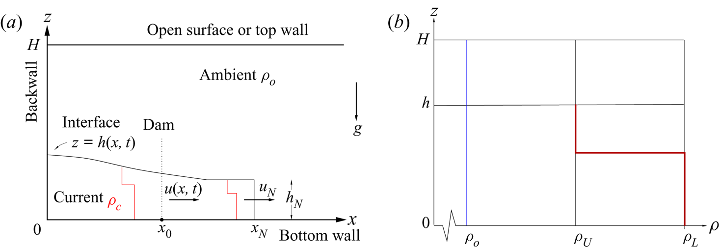
We consider the propagation over a horizontal bottom which develops when a given volume of vertically stratified fluid is released into an ambient fluid of constant density. The motion starts from rest by release of the dense fluid from a lock of height  $h_0$ and length
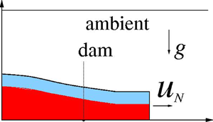
 $x_0$, and is assumed two-dimensional (2-D) (the velocity of the current has no lateral component). The typical configuration is sketched in figure 1. We assume that the density in the lock (and hence in the resulting GC) varies with height, and that the Reynolds number of the flow (defined below) is large.
Schematic description of the GC system (a), and the two-layer stratification (b).

The previous investigations of stratified GCs released from behind a lock into an ambient of constant density were considered by Gladstone et al. (Reference Gladstone, Ritchie, Sparks and Woods2004), Dai (Reference Dai2017) and Wu & Dai (Reference Wu and Dai2019). These works focus, mainly, on laboratory experiments produced for two-layer stratified currents released from the lock: a bottom layer of thickness  $H_L h_0$ (
 $H_L \in (0, 1)$) and density
 $\rho _L$ and an upper layer of thickness
 $(1-H_L) h_0$ and density
 $\rho _U$. The ambient fluid is of density
 $\rho _o=$ const., where
 $\rho _{o} < \rho _U < \rho _L$, and height
 $H h_0$, where
 $H \ge 1$. An inspection of the problem reveals that there are many free input parameters that can vary in significant ranges. The available experimental studies have provided useful insights into the influence of the parameters. However, experiments are an expensive tool that usually covers a limited range of parameters, and the extrapolation of the conclusion to other cases is problematic. For example, all the experiments are for a full-depth lock,
 $H=1$; what will happen to a half-depth lock
 $H=2$ is open to speculation. The general understanding and prediction of such systems are very difficult without a simplified mathematical model. The objective of this paper is to close this gap of knowledge. To this end we develop a one-layer shallow-water model, whose solution reveals the general behaviour in a systematic way. We illustrate the model for the two-layer stratification (as in the experiments) and keep in mind that counterpart results can also be obtained for more complex internal stratifications.
The structure of the paper is as follows. In § 2 we formulate the model for GCs of a general internal stratification. The general insights (slumping, similarity and transition to viscous regime) are presented in § 3. Comparisons with the available two-layer experiments are presented in § 4, followed by some concluding remarks in § 5.
2. Formulation
The typical 2-D GC system is sketched in figure 1. Again, the current was released from a lock of height of  $h_{0}$ and length
 $x_{0}$ into an ambient fluid of density
 $\rho _{o}$ and height
 $H h_0$ (and recall that
 $H \ge 1$ is the dimensionless ambient-to-lock height ratio). The fluid in the lock is denser than the ambient, and stratified from
 $\rho _L$ at the bottom
 $z=0$ to
 $\rho _U$ at the interface
 $z = h_0$. Gravity acts in the
 $-z$ direction. After release from the lock, the dense stratified fluid propagates in the
 $x$ direction.
We use  $\rho _{o}$ as the reference density. We assume a stable stratification, and hence
 $\rho _{L} - \rho _{o}$ is the maximal density difference in the system and is used as the reference quantity for the density variations in the system. We define
 \begin{equation} \epsilon = {(\rho_{L}-\rho_{o}})/{\rho_{o}}, \end{equation}
and assume a Boussinesq system  $\epsilon \ll 1$. The reduced gravity is defined by
 \begin{equation} g' = \epsilon g, \end{equation}
where  $g$ is the gravitational acceleration. We keep in mind that this
 $g'$ is based on the largest density difference; the presence of stratification is expected to also influence the buoyancy driving effect.
As a measure of the importance of the internal stratification, we introduce the parameter  $\sigma$, which is a given constant in the range
 $[0,1]$, defined as follows:
 \begin{equation} \sigma = ({\rho_{L}-\rho_{U}})/({\rho_{L}-\rho_{o}}) , \quad \text{i.e. } ({\rho_{L}-\rho_{U}})/\rho_{o} = \sigma \epsilon. \end{equation}
The case  $\sigma = 0$ means no stratification (the usual homogeneous current), while
 $\sigma = 1$ means that the current matches the density of the ambient at the interface
 $z = h$ (see figure 1). In addition, it is necessary to specify the
 $z$-profile of the stratification. Here we introduce a major assumption.
We conceive the GC as a smooth spread-out of the layered reservoir such that there is the same velocity  $u(x,t)$ across the depth
 $h(x,t)$ of the GC. This implies the formation of a sharp nose (front jump)
 $x = x_N(t)$ of speed
 $u_N(t)$, and the preservation of the density distribution function denoted by
 $R(\eta )$. To be specific, using the definitions above, we express the density of the current (subscript
 $c$) as
 \begin{equation} \rho_{c} = \rho_{o}[ 1+\epsilon ( 1-\sigma R(\eta) ) ], \end{equation}
where  $\eta = {z}/{h} \in [0,1]$ and
 $R(\eta )$ is a known function which is actually defined by the given initial stable stratification in the lock. In general, the stable
 $R$ increases from
 $R(0)=0$ to
 $R(1)=1$, and may be discontinuous. We keep in mind:
 $\eta$ and
 $\rho _c$ are functions of
 $x,t$.
This representation of the GC is a bold idealization of the laboratory observations (Gladstone et al. Reference Gladstone, Ritchie, Sparks and Woods2004; Dai Reference Dai2017; Wu & Dai Reference Wu and Dai2019) which indicate some tendencies of separation and mixing between the dense fluids after release. On the other hand, the experiments reveal a consistent behaviour of propagation that demonstrates the dominance of a depth-averaged dynamics driven by the local buoyancy. The present kinematic description of the current allows the derivation of a self-contained dynamic model that predicts the behaviour for realistic initial conditions, with fair agreement with the measured data. As shown later, the resulting flow is in general stable according to the interfacial Richardson number, which adds credence to the model.
We hope that further research will provide a sharper justification of the model, as well as improvements. By a trial-and-error process we have considered several other modelling scenarios, including separation of layers and fast mixing. These were discarded because we encountered inconsistencies and/or the need for debatable empirical closures. We do not claim that other models are necessarily impossible or less accurate than the present one; we just mention that we could not find a reliable competitor.
The Reynolds number of the horizontal flow,  $Re = U h_0/\nu$, where
 $U$ is a typical speed to be specified later, is assumed to be large, and hence the flow dynamics is dominated by a balance between buoyancy and inertial forces. We use a one-layer shallow-water (SW) model. The motion takes place in the layer of the current only,
 $0 \leq x \leq x_{N}$ and
 $0 \leq z \leq h(x,t)$. We need two equations for the thickness (height) of the current,
 $h(x,t)$ and the
 $z$-averaged velocity
 $u(x,t)$. The volume-continuity balance is as in the standard case; the novelty is in the momentum balance and nose-jump condition, which are affected by the internal stratification.
The hydrostatic balances  $\partial p_{i}/\partial z = -\rho _{i}g,$ where
 $i=a$ (ambient) or
 $i=c$ (current), with
 $\rho _a = \rho _{o}$ and
 $\rho _c$ given by (2.4), upon
 $z$-integration, yield
 \begin{gather} p_{a}(z,t) = -\rho_{o}gz + C; \end{gather}
 \begin{gather}p_{c}(x,z,t) = -\rho_{o}g \left[ (1+\epsilon)z - \epsilon\sigma h I(\eta)\right]+f(x,t), \quad \text{where } I(\eta) = \int_{0}^{\eta}R(\bar{\eta}) \, \textrm{d} \bar{\eta}. \end{gather}
The ‘constant of integration’ function  $f(x,t)$ is then obtained by imposing pressure continuity
 $p_a(z=h)=p_c(z=h)$, upon which (2.5) and 2.6) give
 \begin{equation} p_c(x,z,t) = -g\rho_o[ (1+\epsilon)z - \epsilon\sigma h (I(\eta)-I(1))- \epsilon h ] + C, \end{equation}
where the constant  $C$ is arbitrary. We thus obtain from (2.7)
 \begin{equation} \frac{\partial p_c}{\partial x} = g'\rho_o [ 1 - \sigma \{R(\eta)\,\eta + I(1)-I(\eta)\} ] \frac{\partial h}{\partial x}. \end{equation}
Consequently, for the  $z$-averaged (over the layer of thickness
 $h$) motion, the
 $x$-pressure driving effect is expressed by
 \begin{equation} \frac{\overline{\partial p_{c}}}{\partial x}(x,t) = \rho_o [ g' ( 1 - \sigma \tilde{R}) ] \frac{\partial h}{\partial x}, \end{equation}
where  $\tilde {R}$ is a constant given by
 \begin{equation} \tilde{R} = I(1)+ \int_{0}^{1} [ R(\eta)\,\eta - I(\eta) ] \, \textrm{d} \eta. \end{equation}
It can be shown that  $0 \le \tilde {R} \le 1$ for any acceptable stratification
 $R(\eta )$.
We recall that (2.9) is the driving buoyancy effect in the dense GC. The right-hand side of this result demonstrates that the effective reduced gravity is  $g'(1 - \sigma \tilde {R})$. As expected, the presence of stratification (
 $0<\sigma <1$) weakens the driving force, but the influence of
 $\sigma$ is constrained by integrals of the stratification profile (the coefficient
 $\tilde {R} \le 1$). Taking this into account, we scale the dynamics using the reference speed and time given by
 \begin{equation} U = [g'(1 - \sigma \tilde{R}) h_{0} ]^{1/2}; \quad T = {x_{0}}/{U}. \end{equation}
Then we switch the dimensional variables (denoted by asterisks) to dimensionless variables defined as follows:
 \begin{equation} \{ x^{*}, z^{*}, h^{*}, H^{*}, t^{*}, u^{*}\} = \{ x_{0}x, h_{0}z, h_{0}h, h_{0}H, Tt, Uu \}. \end{equation}
The  $z$-averaged SW equations have been derived and used widely in the context of GCs (e.g. Ungarish Reference Ungarish2009). The stratification has no effect on the volume continuity equation. In the Boussinesq case, the inertia terms are also not affected. The only modification of the momentum balance is in the pressure-driving; see (2.9). Interestingly, the scaling (2.11a,b) accommodates this change. In scaled form we recover the standard system of equations for the height
 $h(x,t)$ and averaged velocity
 $u(x,t)$:
 \begin{equation} \left( \begin{array}{c} h_{t} \\ u_{t} \end{array} \right) + \left( \begin{array}{cc} u & h \\ 1 & u \end{array} \right) \left( \begin{array}{c} h_{x} \\ u_{x} \end{array} \right) = \left( \begin{array}{c} 0 \\ 0 \end{array} \right). \end{equation}
The system is hyperbolic with the characteristic relationships
 \begin{equation} h^{-1/2}\, \textrm{d} h \pm \textrm{d} u = 0 \quad \text{on } \frac{\textrm{d}\kern0.8pt x}{\textrm{d} t} = \lambda_{\pm} = u \pm h^{1/2}. \end{equation}
The initial conditions in the lock  $x \in [0,1]$ are
 $h=1, u=0$ at
 $t=0$, and
 $x_N(t=0) =1.$ The velocity boundary condition is
 $u(t, x=0) = 0$ (at the backwall); to close the solution, the boundary condition at the nose is also needed.
The nose is a moving discontinuity (shock) between a non-stratified domain and a stratified domain. Since no rigorous jump condition is available for such cases, Ungarish & Huppert (Reference Ungarish and Huppert2002) introduced the correlation (in dimensional form)
 \begin{equation} u_N = Fr (a)\, \large ( [ p_c(x=x_N, z=0) - p_a(x=x_N, z=0)] / \rho_{o} \large )^{1/2}, \end{equation}
where  $a = h_N/H$ and
 $Fr(a)$ is an off-the-shelf Froude-number formula for a classical GC. This correlation has been used for modelling Boussinesq currents and intrusions in stratified circumstances and produced good agreement with realistic data. The interpretation is that the pressure difference that drives the jump is counterbalanced by the dynamic reaction
 $\propto \rho _{o} u_N^2$. The dynamic flow depends mostly on the geometry represented by
 $a=h_N/H$, and this implies that the coefficient
 $Fr(a)$ is unaffected by the stratification. The previous studies indicate that the semi-empirical
 $Fr(a)$ of Huppert & Simpson (Reference Huppert and Simpson1980) (see (2.18) below) is a convenient formula for progress.
We adopt (2.15). For the pressure difference we use (2.5) and (2.7) with  $h=h_N$, then scale according to (2.11a,b) and (2.12). We obtain the dimensionless jump condition
 \begin{equation} u(x = x_{N}) = u_{N} = Fr(h_{N}/H) \,\varPsi \,h_{N}^{1/2}, \end{equation}
where  $\varPsi$ is the stratification factor constant given by
 \begin{equation} \varPsi = \left [ \frac{1-\sigma I(1)}{1-\sigma \tilde{R}} \right]^{1/2}, \end{equation}
and
 \begin{equation} Fr(h_{N}/H) = \left\{ \begin{array} {@{}cc} 0.5 ({h_{N}}/{H})^{-1/3}, & 0.075 \leq h_{N}/H \leq 1, \\ 1.19, & 0 \le h_{N}/H < 0.075. \end{array} \right . \end{equation}
(The formulation remains valid for other  $Fr$ formulas.) Integration of
 $u_N \textrm {d} t$ gives
 $x_N$.
3. General results
The formulation (2.13), (2.16)–(2.18) is expected to predict the propagation for various internal stratifications expressed by  $\sigma$ and
 $R(\eta )$. Some general insights can be derived:
1. Collapse of input parameters. We observe that, in scaled form, the solution of the equations and associated boundary conditions depends only on (i) the height ratio  $H$, and (ii) the stratification factor
 $\varPsi$.
2. Initial slumping stage. A dam-break analysis of the hyperbolic system reveals that there is an initial slumping phase of propagation with constant nose height  $h_{N}$ and speed
 $u_{N}$, over a significant distance (
 $x_N \sim 3$–
 $4$). These
 $h_N, u_N$ values can be calculated analytically. We integrate (2.14) for
 $u(h)$ along
 $\lambda _{+}$ from a point in the still lock domain (where
 $u=0$ and
 $h=1$) to the point where
 $u=u_N, h= h_N$. On the other hand, that last point must satisfy the jump condition (2.16). This intersection of
 $u_N$ values gives
 \begin{equation} u_{N} = 2(1-h_{N}^{1/2}) = Fr(h_{N}/H) \, \varPsi \, h_{N}^{1/2}. \end{equation}
Recall that  $\varPsi$ and
 $H$ are constants,
 $Fr(h_N/H)$ is given by (2.18) and
 $\varPsi$ is given by (2.17). The solution of (3.1) provides first
 $h_{N}$ (by a simple iteration) and next
 $u_{N}$. Again, it is evident that the flow depends only on
 $H$ and
 $\varPsi$.
3. Similarity solution. The similarity solution is relevant for large times after release. In this stage the current is already thin,  $h_N/H \ll 1$, and therefore we consider
 $Fr$ to be a constant (
 $\approx Fr(0) = 1.19$). Taking into account the boundary condition (2.16) at the nose, we assume the similarity solution to be of the following form:
 \begin{equation} x_{N}(t) = K t ^{\beta}; \quad h(y,t) = (\dot{x}_{N})^{2}\mathcal{H}(y); \quad u(y,t) = \dot{x}_{N}\mathcal{U}(y), \end{equation}
where  $y = x/x_N \in [0,1]$,
 $\mathcal {U}(1)=1$,
 $\mathcal {H}(1) = (Fr\, \varPsi )^{-2}$, and the upper dot denotes time derivative. Using (3.2a–c) and volume conservation
 $\int _{0}^{x_{N}(t)} h(x,t)\, \textrm {d} x = 1$, we find
 $\beta = {2}/{3}$.
Then, by substitution of (3.2a–c) into (2.13) and (2.16), we obtain
 \begin{equation} \mathcal{U}(y) = y; \quad \mathcal{H}(y) = \frac{1}{(Fr \,\varPsi)^2} - \frac{1}{4} + \frac{1}{4}y^{2}. \end{equation}
Finally, combining the volume conservation with the previous results for  $\beta$ and
 $\mathcal {H}(y)$, we calculate
 $K$. The result is
 \begin{equation} K = \left( \frac{27}{2}\, \frac{Fr^2 \, \varPsi^2}{6-Fr^2 \, \varPsi^2} \right)^{1/3}. \end{equation}
Inspection of the results points out the following: (i) A larger  $\varPsi$ means a faster and thinner current in the developed stage. (ii) The present solution is restricted to
 $\varPsi \le 2/Fr$; for larger
 $\varPsi$ the function
 $\mathcal {H}$ (and hence
 $h$) attains negative non-physical values at small
 $y$ (see (3.3b)). This may indicate the formation of a ‘bare spot’. However, we shall not elaborate on this issue because that restriction on
 $\varPsi$ is not severe, as shown later. (iii) The solution has ‘virtual origin’ because it admits the addition of an arbitrary constant to
 $t$.
4. Transition to viscous regime. The importance of viscous friction in the motion of the current increases with time and distance of propagation. We estimate the inertia per unit volume as  $\rho _{o} (u u_x)^\ast$ and the viscous force per unit area as
 $\rho _{o} \nu (u/h)^\ast$ (dimensional). Upon integration, the ratio of the inertial
 $F_I$ to the viscous
 $F_V$ forces, for the entire GC, in dimensionless form, yields
 \begin{equation} \frac{F_{I}}{F_{V}} = \left(\frac{Uh_0}{\nu} \right) \frac{h_{0}}{x_{0}}\, \frac{\displaystyle\int_{0}^{x_{N}}uu_{x}h\, \textrm{d}\kern0.8pt x}{\displaystyle\int_{0}^{x_{N}}(u/h)\, \textrm{d}\kern0.8pt x}= Re \frac{h_{0}}{x_{0}} \, \theta(t) = Re \frac{h_{0}}{x_{0}} \, \tilde{\theta}(x_N), \end{equation}
where, again,  $Re = U h_0/\nu$. The dimensionless
 $\theta$ and
 $\tilde{\theta}$ are expected to be
 $\sim 1$ initially, and to decrease significantly during propagation. This can be calculated analytically for the developed self-similar stage. Substitution of (3.2a–c)–(3.4) into the integrals of (3.5) and some algebra give
 \begin{equation} \tilde{\theta}(x_N) = C_V\, x_{N}^{-7/2}, \end{equation}
where
 \begin{equation} C_V = \frac{8}{243} K^{15/2} \left({c + \frac{1}{8}} \right) \left[{\ln \left(1+\frac{1}{4c} \right)} \right]^{-1} \quad \textrm{and} \quad c = \frac{1}{(Fr \, \varPsi)^2} - \frac{1}{4}. \end{equation}
The inertial–buoyancy model is expected to be relevant for  $F_{I}/F_{V} > 1$. The length
 $x_N$ when
 ${F_{I}}/{F_{V}} = 1$ is denoted by
 $x_V$, and can be defined as the transition to the viscous regime. Combining (3.5) and (3.6) we obtain
 \begin{equation} x_{V} = \left( Re\frac{h_0}{x_0}C_V \right)^{2/7}. \end{equation}
This provides a practical evaluation of  $x_V$ for a realistic GC of given internal stratification and
 $Re(h_0/x_0)$. The values of
 $\varPsi$ and
 $K$ are given by (2.17) and (3.4), and
 $Fr = Fr(0) = 1.19$.
4. Two-layer stratified current
The clear-cut situation, for which good experimental data are available, is the two-layer stratified current. As set by the lock, the fluid of density  $\rho _L$ occupies
 $0<\eta <H_L$, and the less-dense fluid with density
 $\rho _{U}$ occupies
 $H_L < \eta \leq 1$ (see figure 1). In this case
 \begin{equation} R(\eta) = \left\{ \begin{array}{@{}cc} 0, & 0 \leq \eta \leq H_L;\\ 1, & H_L \lt \eta \leq 1. \end{array} \right. \end{equation}
The integrals  $I(\eta )$ and
 $\tilde {R}$ (see (2.6) and (2.10)) are simple expressions. In particular,
 \begin{equation} I(1) = 1-H_L; \quad \tilde{R} = 1-H_L^2; \quad \varPsi = \left[\frac{1-\sigma(1-H_L)}{1-\sigma(1-H_L^2)} \right]^{1/2}. \end{equation}
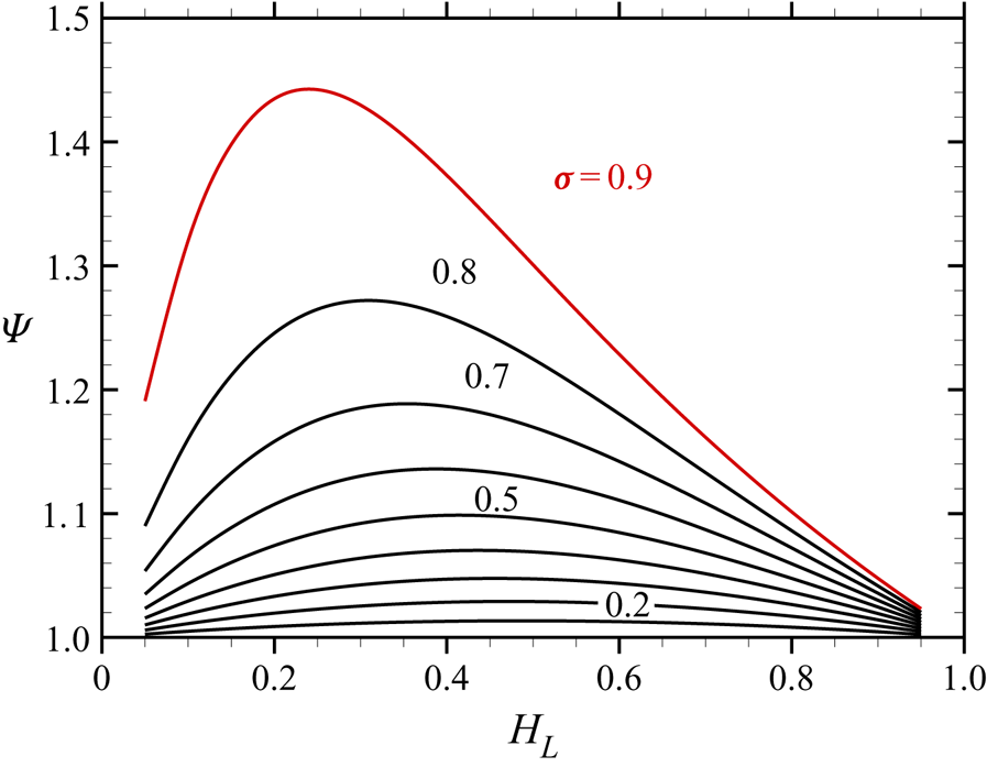
The behaviour of the stratification factor  $\varPsi$ is shown in figure 2. For the classical current
 $\sigma = 0$,
 $\varPsi =1$. For the stratified current,
 $\varPsi >1$; however, the increase is quite small for
 $\sigma <0.7$, less than
 $20\,\%$. This indicates that the effect of the internal stratification is quite modest in many practical cases.
Values of  $\varPsi$ vs
 $H_L$ for
 $\sigma = 0.1, 0.2,\ldots ,0.9$ (for two-layer stratification).

For strong stratification,  $\sigma > 0.9$,
 $\varPsi$ may become significantly larger than 1. However, we restrict our two-layer predictions to
 $\sigma \le 0.9$ (and thus
 $\varPsi <1.45$) cases. This is because
 $\sigma > 0.9$ cases are practically incompatible with the two-layer stratification concept. When
 $\sigma > 0.9$, the density contrast of the upper layer with the ambient is less than
 $10\,\%$ of the contrast of the lower layer. In a Boussinesq system, this implies that
 $\rho _U$ differs from
 $\rho _{o}$ by less than
 $1\,\%$. We argue that in this case the upper layer should be considered a part of the ambient, not of the current. Stability considerations, presented later, support this insight: the upper layer tends to mix with the ambient when
 $\sigma > 0.9$. In other words, the
 $\sigma > 0.9$ case should be approximated and solved as a classical GC of density
 $\rho _L$ in an ambient of density
 $\rho _{o}$. We admit that this cut-off criterion lacks rigour, and we hope that further research on this problem will produce a more accurate criterion in the future. Note that the
 $\sigma \le 0.9$ restriction also implies the condition
 $\varPsi < 1.45 < 2/Fr(0)$, which has been assumed in the similarity solution as discussed in § 3.
Next, we developed a numerical solver for the system of equations (2.13) with the appropriate initial and boundary conditions. We used the approach reported in Ungarish (Reference Ungarish2009) (where other references are given): cast the system in conservation form, transform the dependent variable  $x$ into
 $y = x/x_N(t)$ (so that the spatial domain of solution is
 $[0,1]$), then apply a finite-difference discretization by a two-step Lax–Wendroff method. The input parameters are the depth ratio
 $H$ and the stratification factor
 $\varPsi$; the results are
 $h(x,t), u(x,t), u_N(t), x_N(t)$. The typical grid for the SW results displayed below has 200 points, with a time step of
 $10^{-3}$. The code is robust: for various stratifications
 $\sigma >0, \varPsi >1$ it worked as in the non-stratified case
 $\sigma =0, \varPsi =1$.
4.1. Comparison with the experiments
The pertinent experiments were performed in rectangular tanks of length  $L$ with saline and fresh water. Typically, Gladstone et al. (Reference Gladstone, Ritchie, Sparks and Woods2004) used
 $(h_0, L)$ of (20 cm, 300 cm) and (40 cm, 600 cm); Dai (Reference Dai2017) and Wu & Dai (Reference Wu and Dai2019) used
 $(h_0, L)$ of (20 cm, 250 cm). All tested GCs were with full-depth lock,
 $H=1$, and started in the inertial regime with
 $Re (h_0/x_0) > 10^3$. Two major configurations should be distinguished: (I) Short lock,
 $h_0/x_0 =2$ in Gladstone et al. (Reference Gladstone, Ritchie, Sparks and Woods2004) and Dai (Reference Dai2017); here the GC was observed over a large dimensionless
 $x_N$ of about 20–30. However, the initial adjustment is more like a column collapse than a dam-break, and hence the slumping phase is obscured. (II) Long lock,
 $h_0/x_0 = 0.2$, in Wu & Dai (Reference Wu and Dai2019), which is compatible from the beginning with the thin-layer assumption, and reveals the slumping phase well. In case (II) experiments, the GC reaches the end of the tank at
 $x_N \approx 2$. The relevant experiments were in the stable
 $\sigma \le 0.9$ domain. (Notation correspondence:
 $1-\sigma$ here equals
 $R_\rho$ of Dai (2017) and
 $\rho ^\ast$ of Gladstone et al.;
 $(1-\sigma )H_L/[(1-\sigma )H_L +H_L]$ here equals
 $R_B$ of Dai and
 $B^\ast$ of Gladstone et al. Wu and Dai use
 $R_R=R_\rho$. The parameters of nose-speed
 $\varPsi$ and of lock-buoyancy
 $R_B = B^\ast$ are physically not connected.) Qualitatively, the present theory predicts the observations well: there is a short initial phase of constant
 $u_N$, which develops into self-similar spread
 $x_N \sim t^{2/3}$ (or
 $x_N^{3/2} \sim t$). The quantitative comparison also shows good agreement, as follows.
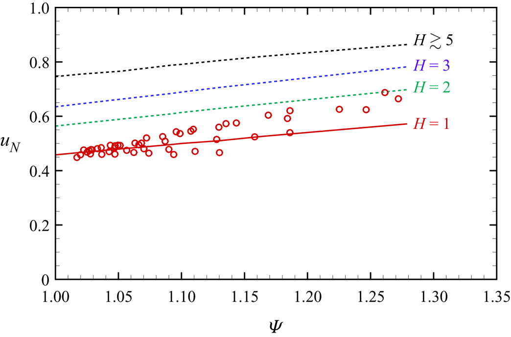
Figure 3 presents a comparison between the present SW slumping  $u_N$ results and experimental data of Wu & Dai (Reference Wu and Dai2019). All 49 reported values (
 $U_f$ of table 2 of that paper) are displayed, in our scaling, as symbols on the plot, according to the corresponding parameter
 $\varPsi$. The data display some scatter about the theoretical line
 $H=1$ (full depth) corresponding to the experimental lock. For
 $\varPsi > 1.2$ the points are consistently above the line, but the discrepancy is only about
 $15\,\%$, and, most encouraging, the predicted trend of increase with
 $\varPsi$ is maintained. (The consistent ‘above the line’ trend is surprising, because the SW
 $u_N$ is expected to be smaller than the data due to friction. The reason for this idiosyncrasy is obscure; we hope that this will be clarified in future studies.) Overall, the collapse of the data to the theoretical curve is very good. We emphasize that this agreement was obtained from self-contained calculations, without the need or use of adjustable parameters. Figure 3 also shows the theoretical slumping speed for part-depth locks: first
 $u_N$ increases with
 $H$ because
 $Fr$ increases according to (2.18); the increase stops for
 $H \gtrsim 5$, where
 $Fr= 1.19$. For any fixed
 $H$,
 $u_N$ increases with
 $\varPsi$. (The
 $H>1$ predictions await experimental verification.)
Values of  $u_N$ in slumping stage vs
 $\varPsi$. Experimental data (symbols) of Wu & Dai (Reference Wu and Dai2019) and the corresponding SW prediction (red full line,
 $H=1$). Also shown: the SW predictions for part-depth release
 $H=2, 3$ and
 $H \gtrsim 5$ (dashed lines).

We proceed to comparisons with the short lock experiments. In this case the propagation of interest is for larger  $t$, over long
 $x_N$ (dimensionless). The available experiments are for
 $H=1$. Therefore, in our scaling, as long as the propagation is in the inertial regime, the dominant free parameter of the compared flows is the stratification factor
 $\varPsi$.
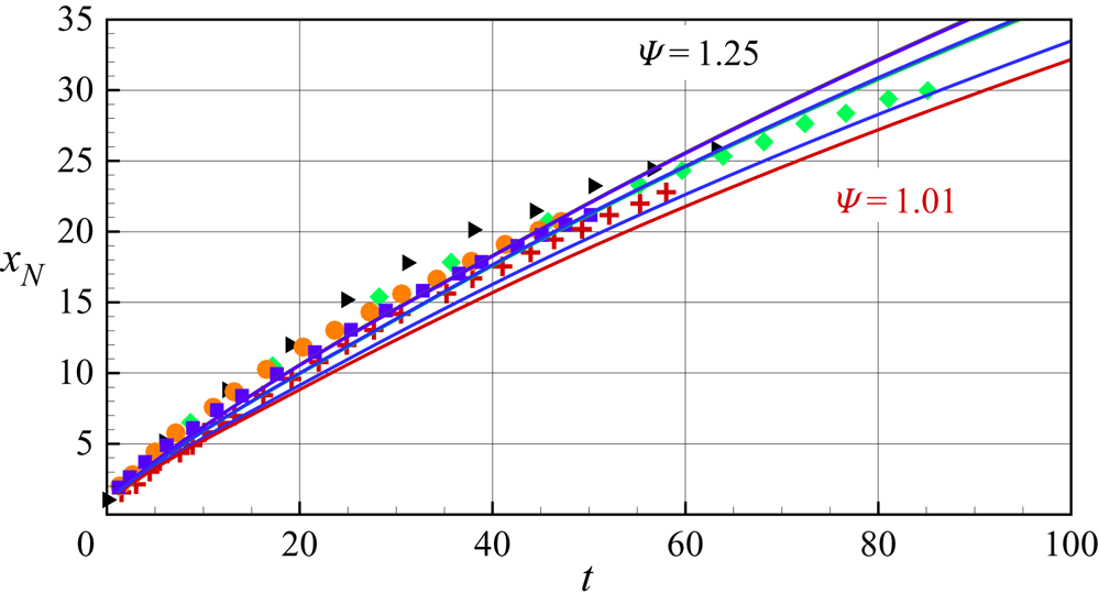
Figure 4 displays  $x_N$ vs
 $t$ for six different experiments: two of Gladstone et al. (Reference Gladstone, Ritchie, Sparks and Woods2004) (B7, B12), with
 $\varPsi = (1.255, 1.170)$, and four of Dai (Reference Dai2017) (E3, D4, K4, K6), with
 $\varPsi = (1.009,1.171,1.250,1.1176$). The experimental symbols collapse on almost the same line. This confirms the theoretical insight that, upon the scaling (2.11a,b) and (2.12), the GCs collapse to the same pattern, governed by the parameter
 $\varPsi$. A close inspection of the recorded trajectories (the symbols) reveals that a larger value of
 $\varPsi$ corresponds to a faster GC. This is in accord with the prediction of the model, as shown by the theoretical lines. The discrepancy between the data and theoretical lines can be attributed to the initial incompatibility of the
 $h_0/x_0 =2$ situation (in all experiments) with the ‘thin current’ concept of the theory. This incompatibility is adjusted in the later motion, and overall the
 $x_N$ discrepancies are only a few per cent, over a quite long propagation of at least 20 units (the data are limited by the length of the laboratory tank). The effect of
 $\varPsi$ is more pronounced on the theoretical lines than on the real data shown in this figure; this discrepancy is evidently a result of the short-lock effect, because in the long-lock case of figure 3 the effect of
 $\varPsi$ on the data is sharper.
SW model (lines) and experimental data (symbols) for  $x_{N}$ vs
 $t$. Dai: E3 ( + red); D4 (
 $\ast$ green); K4 (
 $\circ$ yellow); K6 (
 ${{\Box}}$ blue). Gladstone et al.: B12 (
 $\diamond$ cyan); B7 (
 $\triangleright$ black). The lines of K6, D4 and B12 collapse to the cyan line, because
 $\varPsi \approx 1.17$; the lines of B7 and K4 collapse to the black line, because
 $\varPsi \approx 1.25$.

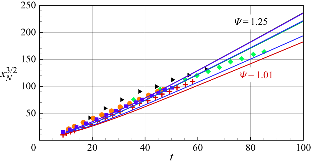
In figure 5 we verify the tendency to self-similar propagation. According to § 3,  $x_{N}^{3/2}$ is expected to become a straight line of
 $t$ at some large
 $t$. The SW finite-difference results attain this behaviour for
 $t > 10$, and the data (symbols) also collapse accordingly. However, the points of experiment B12 (
 $\diamond$ cyan) lag behind the similarity line for
 $t >65, x_N >26$. This indicates a speed reduction due to the transition to the viscous regime. Indeed, according to (3.8),
 $x_V = 27$ for experiment B12, while for all other cases shown in figure 5 the predicted
 $x_V$ is beyond the end of the tank. We infer that the theoretical
 $x_V$ estimate is useful and reliable, but there are not sufficient data for a sharp comparison.
Similarity behaviour  $x_{N}^{3/2}$ vs
 $t$. Notation as in caption of figure 4.

In the presence of three densities, some interfacial instabilities and mixing/entrainment are expected. To estimate the importance of this effect we discern between two Richardson numbers,  $Ri_L$ and
 $Ri_U$, for the interfaces of the lower and upper layers (with the lighter fluid above). Roughly, the shear
 $\omega = \partial u^\ast / \partial z^\ast \approx u^\ast /h^\ast$ is the same in both layers, and the stratification frequencies (dimensional)
 ${\mathcal {N}}^2$ are
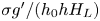 $\sigma g'/(h_0 h H_L)$ and
 $(1-\sigma ) g'/[h_0 h (1-H_L)]$ in the lower and upper layers. Since the shear
 $u/h$ increases with
 $x$, the most unstable domain is expected at the nose where
 $(u^2/h)^\ast = (Fr \varPsi )^2 U^2/h_0$. After some algebra, the relevant-for-stability ratio
 $({\mathcal {N}}/\omega )^2$ yields
 \begin{gather} Ri _L = \sigma (Fr^2 H_L [1 - \sigma (1-H_L) ] )^{-1}; \end{gather}
 \begin{gather} Ri_U = (1-\sigma) (Fr^2 (1-H_L) [1 - \sigma (1-H_L) ] )^{-1}. \end{gather}
A closer inspection shows that for  $Fr < 1.2$ (as used here), both
 $Ri$ are larger than 0.25 in most of the range of interest. The
 $Ri<0.25$ exceptions are the following: (1) When
 $\sigma > 0.9$ the upper layer is expected to mix with the ambient; this may cause a significant change from the assumption that the current is of thickness
 $h$. However, this difficulty is practically relaxed by our previous decision to restrict our prediction to
 $\sigma \le 0.9$ cases. (2) For
 $\sigma < 0.3 H_L$ the lower and upper layers tend to mix; this, however, cannot significantly influence the
 $z$-averaged flow, because in this case both layers are of close densities, and, even upon full local mixing between the
 $\rho _L H_L$ and
 $\rho _U (1-H_L)$ domains, the decrease of the original
 $\epsilon$ is bounded by
 $0.3 H_L (1-H_L) \le 7.5\,\%$. Since
 $u_N \propto \epsilon ^{1/2}$ the effect is small. We conclude that the estimates of
 $Ri$ indicate that interfacial instabilities can produce only weak mixing effects; therefore, a model based on
 $z$-average of unmixed layers is expected to be a good approximation to the realistic flow. The agreements reported above support this conclusion.
5. Concluding remarks
We presented a SW model that provides a compact prediction tool for GCs released from a lock with density stratification, from the initial slumping stage to the transition into the viscous regime. The new theory compares well with the available two-layer experimental data. Needless to say, the present simplified theory cannot reproduce all the complicated details which have been nicely documented in the experimental papers, such as interface billows, local mixing and tendency of separation between the layers. On the other hand, the experiments did not provide data for testing the part-depth lock influence, nor the transition to the viscous regime (with one exception). The theory can be straightforwardly extended to other stratifications, such as the addition of a third layer (with either an intermediary constant density or a smooth transition between the upper and lower). We hope that the present paper will motivate further work on this problem, and in particular experiments for part-depth release, a more accurate understanding of the stability and mixing issues, and more sophisticated theoretical models (with friction, entrainment and drag effects).
Declaration of interests
The authors report no conflict of interest.