1 Introduction
Dense granular flows display many manifestations of grain-size dependence in which cooperative effects at the microscopic grain level have an observable effect on the macroscopic flow phenomenology – such as wide shear bands in split-bottom flow (Fenistein & van Hecke Reference Fenistein and van Hecke2003; Fenistein, van de Meent & van Hecke Reference Fenistein, van de Meent and van Hecke2004), secondary rheology of intruders (Nichol et al. Reference Nichol, Zanin, Bastien, Wandersman and van Hecke2010; Reddy, Forterre & Pouliquen Reference Reddy, Forterre and Pouliquen2011) and the thickness dependence of the flow threshold in shallow inclined plane flow (Pouliquen Reference Pouliquen1999; Silbert, Landry & Grest Reference Silbert, Landry and Grest2003; Weinhart et al. Reference Weinhart, Thornton, Luding and Bokhove2012). Another class of phenomenology affected by cooperativity is dense granular heap flow, such as the flows that arise during avalanches and landslides, in flows down chutes or in rotating drums. Dense granular heap flow is notable because both rapid, fluid-like flow and slow, quasi-static flow are evident in a single configuration. Steady flow fields are characterized by a rapidly flowing layer localized at the free surface with very slow flow beneath (Lemieux & Durian Reference Lemieux and Durian2000; Komatsu et al. Reference Komatsu, Inagaki, Nakagawa and Nasuno2001; Taberlet et al. Reference Taberlet, Richard, Valance, Losert, Pasini, Jenkins and Delannay2003; MiDi Reference MiDi2004; Jop, Forterre & Pouliquen Reference Jop, Forterre and Pouliquen2005; Jop Reference Jop2006; Jop, Forterre & Pouliquen Reference Jop, Forterre and Pouliquen2007; Crassous et al. Reference Crassous, Métayer, Richard and Laroche2008). The thickness of the rapidly flowing surface layer is strongly dependent on the overall flow rate. Due to cooperative effects, the rapid surface flow induces creeping flow beneath (Komatsu et al. Reference Komatsu, Inagaki, Nakagawa and Nasuno2001). (Following the terminology of Komatsu et al. (Reference Komatsu, Inagaki, Nakagawa and Nasuno2001), we use the term creep to describe very slow, quasi-static flow.) The creeping flow decays exponentially with the distance from the free surface. In contrast to the thickness of the surface layer, the characteristic decay length of the creeping flow is independent of the overall flow rate (Jop et al. Reference Jop, Forterre and Pouliquen2007).
Simultaneously capturing both the rapid surface flow and the quasi-static creeping flow with a continuum model has posed a significant challenge and remains an open research question in granular physics. A well-regarded approach, which serves as our starting point, is the inertial rheology (MiDi Reference MiDi2004; da Cruz et al.
Reference da Cruz, Emam, Prochnow, Roux and Chevoir2005; Jop et al.
Reference Jop, Forterre and Pouliquen2005; Kamrin Reference Kamrin2010), which may be understood through basic dimensional arguments. Consider a quasi-monodisperse granular system with mean grain diameter,
 $d$
, and grain material density,
 $\unicode[STIX]{x1D70C}_{s}$
, subjected to homogeneous planar shear with pressure,
 $P$
, and shear stress,
 $\unicode[STIX]{x1D70F}$
. The consequent shear strain rate,
 $\dot{\unicode[STIX]{x1D6FE}}$
, may be non-dimensionalized as
 $I=\dot{\unicode[STIX]{x1D6FE}}\sqrt{d^{2}\unicode[STIX]{x1D70C}_{s}/P}$
– referred to as the inertial number. The inertial number operates as a normalized strain rate and represents the ratio of the microscopic time scale associated with particle motion,
 $\sqrt{d^{2}\unicode[STIX]{x1D70C}_{s}/P}$
, to the macroscopic time scale of applied deformation,
 $1/\dot{\unicode[STIX]{x1D6FE}}$
(MiDi Reference MiDi2004). The local inertial rheology – local in the sense that it relates the local stress state to the local state of strain rate at a point – then asserts that the stress ratio,
 $\unicode[STIX]{x1D707}=\unicode[STIX]{x1D70F}/P$
, and the inertial number,
 $I$
, are related through a one-to-one constitutive relationship,
 $\unicode[STIX]{x1D707}=\unicode[STIX]{x1D707}_{loc}(I)$
. A common functional form for the local inertial rheology – appropriate for modelling the rapidly flowing surface layers described above – was proposed by Jop et al. (Reference Jop, Forterre and Pouliquen2005):
 $$\begin{eqnarray}\unicode[STIX]{x1D707}=\unicode[STIX]{x1D707}_{loc}(I)=\unicode[STIX]{x1D707}_{s}+\frac{\unicode[STIX]{x1D707}_{2}-\unicode[STIX]{x1D707}_{s}}{I_{0}/I+1},\end{eqnarray}$$
where
 $\unicode[STIX]{x1D707}_{s}=\unicode[STIX]{x1D707}_{loc}(I\rightarrow 0)$
is the static yield value,
 $\unicode[STIX]{x1D707}_{2}=\unicode[STIX]{x1D707}_{loc}(I\rightarrow \infty )$
is the maximum value of
 $\unicode[STIX]{x1D707}$
asymptotically approached as
 $I$
increases and
 $I_{0}$
is a dimensionless parameter characterizing the nonlinear, rate-dependent response. The subsequent work of Jop, Forterre & Pouliquen (Reference Jop, Forterre and Pouliquen2006) generalized the local rheology (1.1) to three-dimensional flow settings as follows. Denote the symmetric strain-rate tensor as
 $\dot{\unicode[STIX]{x1D6FE}}_{ij}=(1/2)(\unicode[STIX]{x2202}v_{i}/\unicode[STIX]{x2202}x_{j}+\unicode[STIX]{x2202}v_{j}/\unicode[STIX]{x2202}x_{i})$
with
 $v_{i}$
the velocity vector and
 $x_{i}$
the spatial coordinate. Jop et al. (Reference Jop, Forterre and Pouliquen2006) began by assuming that steady, dense flow proceeds at approximately constant volume, so that the strain-rate tensor is deviatoric and
 $\dot{\unicode[STIX]{x1D6FE}}_{kk}=0$
. The equivalent shear strain rate is then defined as
 $\dot{\unicode[STIX]{x1D6FE}}=(2\dot{\unicode[STIX]{x1D6FE}}_{ij}\dot{\unicode[STIX]{x1D6FE}}_{ij})^{1/2}$
. Next, to generalize the stress-related quantities involved in the inertial rheology (1.1) to three dimensions, denote the symmetric Cauchy stress as
 $\unicode[STIX]{x1D70E}_{ij}=\unicode[STIX]{x1D70E}_{ji}$
and define the pressure
 $P=-(1/3)\unicode[STIX]{x1D70E}_{kk}$
, the stress deviator
 $\unicode[STIX]{x1D70E}_{ij}^{\prime }=\unicode[STIX]{x1D70E}_{ij}+P\unicode[STIX]{x1D6FF}_{ij}$
, the equivalent shear stress
 $\unicode[STIX]{x1D70F}=(\unicode[STIX]{x1D70E}_{ij}^{\prime }\unicode[STIX]{x1D70E}_{ij}^{\prime }/2)^{1/2}$
and the stress ratio
 $\unicode[STIX]{x1D707}=\unicode[STIX]{x1D70F}/P$
. Jop’s three-dimensional form of the local inertial rheology then takes the following form:
 $$\begin{eqnarray}\unicode[STIX]{x1D70E}_{ij}=-P\unicode[STIX]{x1D6FF}_{ij}+2\unicode[STIX]{x1D707}_{loc}(I)P\frac{\dot{\unicode[STIX]{x1D6FE}}_{ij}}{\dot{\unicode[STIX]{x1D6FE}}},\end{eqnarray}$$
which assumes that the strain-rate tensor and stress deviator are codirectional. When this constitutive model is applied to steady, dense granular heap flow, aspects of the rapidly flowing surface layer may be accurately captured; however, as evidenced by the calculations of Jop et al. (Reference Jop, Forterre and Pouliquen2006, Reference Jop, Forterre and Pouliquen2007) and Kamrin (Reference Kamrin2010), the model also predicts a static zone beneath the rapidly flowing surface layer. This is because the constitutive relation (1.2) possesses a yield condition in the form of a Drucker–Prager criterion (Drucker & Prager Reference Drucker and Prager1952), in which flow does not occur for
 $\unicode[STIX]{x1D707}<\unicode[STIX]{x1D707}_{s}$
. Since
 $\unicode[STIX]{x1D707}<\unicode[STIX]{x1D707}_{s}$
in the region deep beneath the free surface in dense granular heap flow, the rheology (1.2) predicts that this region is frozen, contrary to experimental observations of exponentially decaying creep flow. In addition to dense heap flow, a decaying flow profile is experimentally observed in creeping regions where
 $\unicode[STIX]{x1D707}<\unicode[STIX]{x1D707}_{s}$
across a variety of configurations, such as annular shear flow (Losert et al.
Reference Losert, Bocquet, Lubensky and Gollub2000; Mueth et al.
Reference Mueth, Debregeas, Karczmar, Eng, Nagel and Jaeger2000; Koval et al.
Reference Koval, Roux, Corfdir and Chevoir2009), planar shear flow with gravity (Siavoshi, Orpe & Kudrolli Reference Siavoshi, Orpe and Kudrolli2006) and split-bottom flow (Fenistein & van Hecke Reference Fenistein and van Hecke2003; Fenistein et al.
Reference Fenistein, van de Meent and van Hecke2004). When applied to these cases, the inertial rheology (1.2) will continue to predict frozen regions with a sharp flow cutoff occurring where
 $\unicode[STIX]{x1D707}=\unicode[STIX]{x1D707}_{s}$
. The failure of the local inertial rheology to capture creeping flow when
 $\unicode[STIX]{x1D707}<\unicode[STIX]{x1D707}_{s}$
stems from the fact that it does not mathematically account for non-local, cooperative effects, which become dominant in this regime.
Motivated by this shortcoming, in recent years, non-local continuum constitutive models for dense granular flow have been developed, aimed at accounting for cooperative effects (e.g. Savage Reference Savage1998; Aranson & Tsimring Reference Aranson and Tsimring2002; Mohan, Rao & Nott Reference Mohan, Rao and Nott2002; Berzi & Jenkins Reference Berzi and Jenkins2011; Bouzid et al. Reference Bouzid, Trulsson, Claudin, Clément and Andreotti2013). While these approaches incorporate non-locality and some have had success in individual geometries, none have been shown to capture the salient aspects of steady, dense granular heap flow. Recently, we proposed a non-local continuum model – called the non-local granular fluidity (NGF) model – inspired by related modelling work in the emulsion community (Goyon et al. Reference Goyon, Colin, Ovarlez, Ajdari and Bocquet2008; Bocquet, Colin & Ajdari Reference Bocquet, Colin and Ajdari2009), which is capable of quantitatively describing a diverse set of slow, boundary-driven inhomogeneous flows (Kamrin & Koval Reference Kamrin and Koval2012; Henann & Kamrin Reference Henann and Kamrin2013), the secondary rheology of intruders (Henann & Kamrin Reference Henann and Kamrin2014a ) and the size dependence of the flow threshold in inclined plane flow (Kamrin & Henann Reference Kamrin and Henann2015). The purpose of this paper is to show that the non-local granular fluidity model is capable of capturing steady, dense granular heap flow – in particular, the coexistence of a rapidly flowing surface layer and a creeping bulk.
The remainder of this paper is organized as follows. In § 2, we discuss the specifics of the NGF model, and in § 3, we apply the model to steady, dense granular flows on a heap between two smooth, frictional side walls. Specifically, in § 3.2, we compare velocity fields predicted by the model with experimentally measured flow fields from the literature for glass beads (Jop Reference Jop2006; Jop et al. Reference Jop, Forterre and Pouliquen2007). Importantly, the material parameters appearing in the NGF model have previously been determined for glass beads (Forterre & Pouliquen Reference Forterre and Pouliquen2003; Jop et al. Reference Jop, Forterre and Pouliquen2005; Henann & Kamrin Reference Henann and Kamrin2013), allowing the NGF model to be applied without parameter adjustment. Then, in § 3.3, we examine the relationships between total flow rate, maximum velocity and surface inclination angle, and in § 3.4, we explore the length scales that characterize the coexistent rapidly flowing and creeping zones. Throughout, our results demonstrate a level of agreement between model predictions and experiments that has not been previously reported. We close with a discussion of the limits of the modelling approach and future research directions in § 4.
2 The non-local granular fluidity model
In this section, we summarize the NGF model for dense, steady granular flow (see Kamrin & Koval Reference Kamrin and Koval2012; Henann & Kamrin Reference Henann and Kamrin2013, Reference Henann and Kamrin2014a
,Reference Henann and Kamrin
b
; Kamrin & Henann Reference Kamrin and Henann2015). Similar to the local inertial rheology, the NGF model is valid for granular systems consisting of grains that are (i) spherical, (ii) quasi-monodisperse with constant mean grain diameter
 $d$
and (iii) stiff and is intended for steady, well-developed flow conditions. (Incorporating particle stiffness into granular rheology is an open research problem. For recent progress on this point, see the works of Campbell (Reference Campbell2014), Singh et al. (Reference Singh, Magnanimo, Saitoh and Luding2015) and Roy, Luding & Weinhart (Reference Roy, Luding and Weinhart2017).) The model consists of three main ingredients: (i) a state parameter, called the granular fluidity, (ii) the flow rule and (iii) the non-local rheology, described in detail below.
-
(i) Granular fluidity: Central to the model is the granular fluidity field – a positive, scalar state variable, denoted as
 $g$
. This state variable is kinematic in nature and characterizes microscopic fluctuations in a flowing granular media. More precisely, Zhang & Kamrin (Reference Zhang and Kamrin2017) showed that the granular fluidity is a kinematic state variable given through the velocity fluctuation,
$\unicode[STIX]{x1D6FF}v$
, the solid volume fraction,
$\unicode[STIX]{x1D719}$
, and the grain size,
$d$
, through the relation
$g=(\unicode[STIX]{x1D6FF}v/d)F(\unicode[STIX]{x1D719})$
, where
$F(\unicode[STIX]{x1D719})$
is a function of only
$\unicode[STIX]{x1D719}$
.
-
(ii) Flow rule: For the case of homogeneous planar shear, the granular fluidity relates the stress ratio,
$\unicode[STIX]{x1D707}=\unicode[STIX]{x1D70F}/P$
, to the consequent shear strain rate,
$\dot{\unicode[STIX]{x1D6FE}}$
, through the following constitutive relation: (2.1)This one-dimensional version of the flow rule may be generalized to three dimensions following a procedure analogous to that used by Jop et al. (Reference Jop, Forterre and Pouliquen2006) to generalize the inertial rheology, discussed in § 1. We define the strain-rate tensor as
$$\begin{eqnarray}\dot{\unicode[STIX]{x1D6FE}}=g\unicode[STIX]{x1D707}.\end{eqnarray}$$
$\dot{\unicode[STIX]{x1D6FE}}_{ij}=(\unicode[STIX]{x2202}v_{i}/\unicode[STIX]{x2202}x_{j}+\unicode[STIX]{x2202}v_{j}/\unicode[STIX]{x2202}x_{i})/2$
– where
$v_{i}$
is the velocity field and
$x_{i}$
is the spatial coordinate. Next, we make the common approximation that well-developed steady flow proceeds at constant volume, so that
$\dot{\unicode[STIX]{x1D6FE}}_{kk}=0$
(Jop et al.
Reference Jop, Forterre and Pouliquen2006; Koval et al.
Reference Koval, Roux, Corfdir and Chevoir2009; Rycroft, Kamrin & Bazant Reference Rycroft, Kamrin and Bazant2009; Kamrin Reference Kamrin2010) and define the equivalent shear strain rate as
$\dot{\unicode[STIX]{x1D6FE}}=(2\dot{\unicode[STIX]{x1D6FE}}_{ij}\dot{\unicode[STIX]{x1D6FE}}_{ij})^{1/2}$
. (Recent work has shown that dilatancy can have an effect on steady flows, leading to secondary flow with magnitude of the order of
${\sim}5\,\%$
of the primary flow (Krishnaraj & Nott Reference Krishnaraj and Nott2016). Since this effect has not yet been reported for steady, dense granular heap flow, we neglect it in the present work.) The Cauchy stress tensor and stress deviator are denoted as
$\unicode[STIX]{x1D70E}_{ij}=\unicode[STIX]{x1D70E}_{ji}$
and
$\unicode[STIX]{x1D70E}_{ij}^{\prime }=\unicode[STIX]{x1D70E}_{ij}-(1/3)(\unicode[STIX]{x1D70E}_{kk})\unicode[STIX]{x1D6FF}_{ij}$
. Then, the equivalent shear stress, pressure and stress ratio are defined through stress-tensor invariants as
$\unicode[STIX]{x1D70F}=(\unicode[STIX]{x1D70E}_{ij}^{\prime }\unicode[STIX]{x1D70E}_{ij}^{\prime }/2)^{1/2}$
,
$P=-\unicode[STIX]{x1D70E}_{kk}/3$
, and
$\unicode[STIX]{x1D707}=\unicode[STIX]{x1D70F}/P$
, respectively. Finally, assuming that the strain-rate tensor and stress deviator are codirectional (Jop et al.
Reference Jop, Forterre and Pouliquen2006; Rycroft et al.
Reference Rycroft, Kamrin and Bazant2009; Kamrin Reference Kamrin2010), the one-dimensional flow rule (2.1) may be expressed in tensorial form as (2.2)Slight deviations from codirectionality have been observed in discrete element simulations, namely
$$\begin{eqnarray}\unicode[STIX]{x1D70E}_{ij}=-P\unicode[STIX]{x1D6FF}_{ij}+2\frac{P}{g}\dot{\unicode[STIX]{x1D6FE}}_{ij}.\end{eqnarray}$$
${\sim}1{-}2\,\%$
non-coaxiality between
$\dot{\unicode[STIX]{x1D6FE}}_{ij}$
and
$\unicode[STIX]{x1D70E}_{ij}^{\prime }$
(Weinhart et al.
Reference Weinhart, Hartkamp, Thornton and Luding2013) and the normal stress differences (Depken et al.
Reference Depken, Lechman, van Hecke, van Saarloos and Grest2007). For recent work incorporating these effects into a rheological model, see Weinhart et al. (Reference Weinhart, Hartkamp, Thornton and Luding2013).
-
(iii) Non-local rheology: With the introduction of the granular fluidity field,
$g$
, an additional field equation is required to relate the fluidity field to the stress field. In a local constitutive approach, the fluidity would be given as an algebraic function of the stress through the stress invariants
$\unicode[STIX]{x1D707}$
and
$P$
. In contrast, in our non-local approach, the granular fluidity,
$g$
, is governed by the following partial differential equation (PDE) (Henann & Kamrin Reference Henann and Kamrin2014b
): (2.3)where
$$\begin{eqnarray}t_{0}\frac{\text{D}g}{\text{D}t}=A^{2}d^{2}\frac{\unicode[STIX]{x2202}^{2}g}{\unicode[STIX]{x2202}x_{k}\unicode[STIX]{x2202}x_{k}}-\left[\unicode[STIX]{x0394}\unicode[STIX]{x1D707}\left(\frac{\unicode[STIX]{x1D707}_{s}-\unicode[STIX]{x1D707}}{\unicode[STIX]{x1D707}_{2}-\unicode[STIX]{x1D707}}\right)g+b\sqrt{\frac{\unicode[STIX]{x1D70C}_{s}d^{2}}{P}}\unicode[STIX]{x1D707}g^{2}\right],\end{eqnarray}$$
$\text{D}(\bullet )/\text{D}t$
is the material time derivative. (Note that the non-local rheology (2.3) shows mathematical similarities to the order-parameter-based rheological approach of Aranson & Tsimring (Reference Aranson and Tsimring2002).) In (2.3),
$t_{0}$
is a constant time scale associated with the dynamics of
$g$
,
$A$
is a constant dimensionless material parameter characterizing non-local effects called the non-local amplitude and the constants
$\unicode[STIX]{x0394}\unicode[STIX]{x1D707}=\unicode[STIX]{x1D707}_{2}-\unicode[STIX]{x1D707}_{s}$
and
$b=\unicode[STIX]{x0394}\unicode[STIX]{x1D707}/I_{0}$
are given through the three constant material parameters
$\{\unicode[STIX]{x1D707}_{s},\unicode[STIX]{x1D707}_{2},I_{0}\}$
appearing in the local inertial rheology (1.1). The mean grain diameter and grain material density continue to be denoted by
$d$
and
$\unicode[STIX]{x1D70C}_{s}$
, respectively, and are constants. During steady, homogeneous flow, the non-local rheology (2.3) reduces to the local inertial rheology, (1.1) and (1.2). To see this, consider homogenous flow in the absence of spatial gradients in
$g$
(
$\unicode[STIX]{x2202}^{2}g/\unicode[STIX]{x2202}x_{k}\unicode[STIX]{x2202}x_{k}=0$
) and for a fixed state of stress
$(\unicode[STIX]{x1D707},P)$
. Then, at sufficiently long time (
$t\gg t_{0}$
),
$g$
evolves to a stable Lagrangian steady state (
$\text{D}g/\text{D}t\approx 0$
), which we denote as
$g_{loc}(\unicode[STIX]{x1D707},P)$
. The nature of the stable steady state,
$g_{loc}(\unicode[STIX]{x1D707},P)$
, depends on the sign of
$(\unicode[STIX]{x1D707}_{s}-\unicode[STIX]{x1D707})$
. For
$\unicode[STIX]{x1D707}\leqslant \unicode[STIX]{x1D707}_{s}$
, the only steady solution is
$g_{loc}=0$
, and it is stable under perturbation in
$g$
. For
$\unicode[STIX]{x1D707}>\unicode[STIX]{x1D707}_{s}$
,
$g_{loc}=0$
remains a steady solution; however, it becomes unstable under perturbation in
$g$
. The stable, steady solution for
$\unicode[STIX]{x1D707}>\unicode[STIX]{x1D707}_{s}$
is
$g_{loc}=\sqrt{P/\unicode[STIX]{x1D70C}_{s}d^{2}}I_{0}(\unicode[STIX]{x1D707}-\unicode[STIX]{x1D707}_{s})/(\unicode[STIX]{x1D707}(\unicode[STIX]{x1D707}_{2}-\unicode[STIX]{x1D707}))$
. Putting the stable solutions together, we have (2.4)We call the stress-dependent function
$$\begin{eqnarray}g_{loc}(\unicode[STIX]{x1D707},P)=\left\{\begin{array}{@{}ll@{}}\displaystyle \sqrt{P/\unicode[STIX]{x1D70C}_{s}d^{2}}I_{0}\frac{(\unicode[STIX]{x1D707}-\unicode[STIX]{x1D707}_{s})}{\unicode[STIX]{x1D707}(\unicode[STIX]{x1D707}_{2}-\unicode[STIX]{x1D707})} & \text{if }\unicode[STIX]{x1D707}>\unicode[STIX]{x1D707}_{s},\\ 0 & \text{if }\unicode[STIX]{x1D707}\leqslant \unicode[STIX]{x1D707}_{s}.\end{array}\right.\end{eqnarray}$$
$g_{loc}(\unicode[STIX]{x1D707},P)$
the local fluidity, since if the granular fluidity,
$g$
, is taken to be given through the function
$g_{loc}(\unicode[STIX]{x1D707},P)$
and combined with the flow rule (2.2), we recover the local inertial rheology, (1.1) and (1.2). Then, in the case of inhomogeneous flows involving spatial gradients in
$g$
, the Laplacian term appearing in (2.3) introduces an intrinsic length scale given through
$d$
, and hence the rheology is non-local in character. In the present work, we are concerned with dense granular flows that are steady in a Lagrangian sense, in which
$t\gg t_{0}$
so that
$\text{D}g/\text{D}t\approx 0$
. However, reducing the dynamical PDE (2.3) to the steady-state case is not as simple as setting the left-hand side to zero because the stability of the
$g=0$
solution depends on the sign of
$(\unicode[STIX]{x1D707}_{s}-\unicode[STIX]{x1D707})$
. In order to obtain a differential relation for
$g$
specialized to the case of steady flow, we allow for gradients in
$g$
but limit attention to small deviation of
$g$
from
$g_{loc}$
for a given state of stress
$(\unicode[STIX]{x1D707},P)$
. The result of such a simplification (see § 4.3.1 of Henann & Kamrin (Reference Henann and Kamrin2014b
) for the details of this calculation) is (2.5)where
$$\begin{eqnarray}g=g_{loc}+\unicode[STIX]{x1D709}^{2}\frac{\unicode[STIX]{x2202}^{2}g}{\unicode[STIX]{x2202}x_{k}\unicode[STIX]{x2202}x_{k}},\end{eqnarray}$$
$g_{loc}(\unicode[STIX]{x1D707},P)$
is the local fluidity function, given through
$(\unicode[STIX]{x1D707},P)$
as in (2.4), and
$\unicode[STIX]{x1D709}(\unicode[STIX]{x1D707})$
is a stress-dependent length scale called the cooperativity length, given by (2.6)Note that in the absence of any stress or flow gradients (
$$\begin{eqnarray}\unicode[STIX]{x1D709}(\unicode[STIX]{x1D707})=A\sqrt{\frac{\unicode[STIX]{x1D707}_{2}-\unicode[STIX]{x1D707}}{\unicode[STIX]{x0394}\unicode[STIX]{x1D707}|\unicode[STIX]{x1D707}-\unicode[STIX]{x1D707}_{s}|}}d.\end{eqnarray}$$
$\unicode[STIX]{x2202}^{2}g/\unicode[STIX]{x2202}x_{k}\unicode[STIX]{x2202}x_{k}=0$
), the steady-state form (2.5) simply reduces to
$g=g_{loc}(\unicode[STIX]{x1D707},P)$
, and the local inertial rheology is recovered, as should be the case for homogeneous steady flow. However, for inhomogeneous flow, the presence of the Laplacian term gives rise to non-local effects – with predictions of the NGF model being size dependent due to the cooperativity length (2.6) being directly proportional to the grain size,
$d$
. In particular, in regions where
$\unicode[STIX]{x1D707}\leqslant \unicode[STIX]{x1D707}_{s}$
, the local fluidity (2.4) is zero, and (2.5) reduces to
$g=\unicode[STIX]{x1D709}^{2}(\unicode[STIX]{x2202}^{2}g/\unicode[STIX]{x2202}x_{k}\unicode[STIX]{x2202}x_{k})$
, which gives rise to creeping flow predictions with a decay length determined by
$\unicode[STIX]{x1D709}$
rather than a sharp flow cutoff. In the simulations of § 3, with a few noted exceptions, we utilize the steady-state form of the NGF model, (2.5) with (2.4) and (2.6), rather than the dynamical form (2.3). We note that the dimensionless parameter
$A$
appearing in (2.6) is the only new material parameter introduced in the steady-state form of the NGF model beyond the local parameters,
$\{\unicode[STIX]{x1D707}_{s},\unicode[STIX]{x1D707}_{2},I_{0}\}$
.














The system of equations described above are then closed by the standard equations of motion
 $$\begin{eqnarray}\frac{\unicode[STIX]{x2202}\unicode[STIX]{x1D70E}_{ij}}{\unicode[STIX]{x2202}x_{j}}+\unicode[STIX]{x1D719}\unicode[STIX]{x1D70C}_{s}G_{i}=\unicode[STIX]{x1D719}\unicode[STIX]{x1D70C}_{s}\frac{\text{D}v_{i}}{\text{D}t},\end{eqnarray}$$
with
 $G_{i}$
the acceleration of gravity (denoted as
 $G$
to differentiate it from the granular fluidity
 $g$
) and
 $\unicode[STIX]{x1D719}$
the solid volume fraction, taken to be 0.62 for randomly close-packed, quasi-monodisperse, spherical grains (Scott Reference Scott1960). Consistent with our assumption of steady, well-developed flow, we neglect the effect of macroscopic inertia, so that (2.7) reduces to
 $$\begin{eqnarray}\frac{\unicode[STIX]{x2202}\unicode[STIX]{x1D70E}_{ij}}{\unicode[STIX]{x2202}x_{j}}+\unicode[STIX]{x1D719}\unicode[STIX]{x1D70C}_{s}G_{i}=0_{i}.\end{eqnarray}$$
The boundary conditions accompanying this boundary-value problem are discussed in the next section in the context of the specific problem of steady dense granular heap flow.
In our previous work, the NGF model has been shown to quantitatively describe a broad set of experimental steady flow data, including all variations of the complex split-bottom family of geometries in addition to annular shear flow and planar shear flow with gravity (Henann & Kamrin Reference Henann and Kamrin2013). The model has also been shown to correctly capture other non-local phenomena such as non-locally induced material weakening, i.e. ‘secondary rheology’ (Nichol et al. Reference Nichol, Zanin, Bastien, Wandersman and van Hecke2010; Reddy et al. Reference Reddy, Forterre and Pouliquen2011), whereby the motion of a boundary removes the yield strength of the material everywhere, permitting far-away loaded objects to creep through the grains when otherwise they would remain static (Henann & Kamrin Reference Henann and Kamrin2014a ). Finally, in Kamrin & Henann (Reference Kamrin and Henann2015), the model has also shown itself able to describe the size-dependent strengthening seen in experiments of gravity-driven flow down a rough inclined plane (Pouliquen Reference Pouliquen1999; Silbert et al. Reference Silbert, Landry and Grest2003; Weinhart et al. Reference Weinhart, Thornton, Luding and Bokhove2012). When discussing the successes of the NGF model, it is also important to note its limits. Although the NGF model can model developing flows and the approach to steady state, it has not been designed to be quantitatively predictive in this regard. In particular, it is not yet known whether the time-dependent term appearing in the dynamical form (2.3) is able to quantitatively capture transient effects, such as those reported by Ries, Brendel & Wolf (Reference Ries, Brendel and Wolf2016). Hence, at present, the NGF model is only appropriate for steady-state conditions. It is also limited to granular systems, in which grains are spherical, quasi-monodisperse and stiff. In what follows, we will apply the model to situations in which these assumptions are valid.
3 Numerical simulations of dense, steady granular heap flow
In this section, we turn to applying the NGF model to the problem of dense, steady granular heap flow. We will compare predictions of the NGF model to experiments in the literature using glass beads (Jop Reference Jop2006; Jop et al.
Reference Jop, Forterre and Pouliquen2007). Regarding the dimensionless material parameters for glass beads
 $\{\unicode[STIX]{x1D707}_{s},\unicode[STIX]{x1D707}_{2},I_{0},A\}$
, the local parameters are taken from well-established data (Forterre & Pouliquen Reference Forterre and Pouliquen2003; Jop et al.
Reference Jop, Forterre and Pouliquen2005):
 $$\begin{eqnarray}\displaystyle \unicode[STIX]{x1D707}_{s}=0.3819,\quad \unicode[STIX]{x1D707}_{2}=0.6435,\quad \text{and}\quad I_{0}=0.279. & & \displaystyle\end{eqnarray}$$
In our previous work (Henann & Kamrin Reference Henann and Kamrin2013), the non-local amplitude for glass beads was calibrated to be
 $$\begin{eqnarray}\displaystyle A=0.48 & & \displaystyle\end{eqnarray}$$
by fitting NGF model predictions to experimental flow fields for dense, quasi-static granular flow in the split-bottom cell (Fenistein & van Hecke Reference Fenistein and van Hecke2003; Fenistein et al.
Reference Fenistein, van de Meent and van Hecke2004). Since the heap flows reported by Jop and coworkers (Jop Reference Jop2006; Jop et al.
Reference Jop, Forterre and Pouliquen2007) also involve dense flows of spherical glass beads, we expect that these material parameter values remain valid and in what follows we continue to use these parameters without adjustment. Further, we take
 $\unicode[STIX]{x1D70C}_{s}=2450~\text{kg}~\text{m}^{-3}$
and
 $d=0.5$
mm in our calculations; however, all results in subsequent sections will be presented in dimensionless form, and hence, the numerical values of
 $\unicode[STIX]{x1D70C}_{s}$
and
 $d$
are inconsequential.
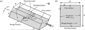
(a) Schematic and (b) computational domain for steady, dense granular heap flow, following the flow configurations used in the experiments of Komatsu et al. (Reference Komatsu, Inagaki, Nakagawa and Nasuno2001) and Jop et al. (Reference Jop, Forterre and Pouliquen2005, Reference Jop, Forterre and Pouliquen2007).

3.1 Flow configuration
To study gravity-driven, dense granular heap flow, we consider the system shown in figure 1(a), consisting of a granular layer of depth,
 $H$
, at an inclination angle,
 $\unicode[STIX]{x1D703}$
, flowing between two smooth, frictional side walls separated by a distance,
 $W$
. The coefficient of sliding friction between the granular media and the side walls,
 $\unicode[STIX]{x1D707}_{wall}$
, is taken to be a constant value and the floor is rough. The component of the acceleration of gravity in the
 $y$
-direction –
 $G\sin \unicode[STIX]{x1D703}$
– then drives flow down the channel – which is very long in the
 $y$
-direction. The expected consequent steady-state flow field – which is invariant along the length of the channel, i.e. the
 $y$
-direction, and decays with depth beneath the surface, i.e. the
 $z$
-direction – is sketched schematically in figure 1(a). The total volume flow rate of granular material down the channel is denoted by
 $Q$
. (In the present work, we use
 $Q$
to denote the total volume flow rate rather than the flow rate per unit width as in Jop et al. (Reference Jop, Forterre and Pouliquen2005, Reference Jop, Forterre and Pouliquen2007).) Note that in experiments the flow rate,
 $Q$
, is typically prescribed, and the free surface inclination angle,
 $\unicode[STIX]{x1D703}$
, follows as a consequence (Jop et al.
Reference Jop, Forterre and Pouliquen2005).
To apply the NGF model to flow in this configuration, we take advantage of the invariance of the steady flow field in the
 $y$
-direction and make an antiplane shear idealization, in which the only non-zero component of velocity is in the
 $y$
-direction, denoted by
 $v$
, and only depends on the
 $x$
and
 $z$
coordinates, i.e.
 $v(x,z)$
, thereby reducing the problem to two dimensions. Under the antiplane shear assumption, the constitutive equation (2.2) implies that the non-zero stress components are
 $\unicode[STIX]{x1D70E}_{xx}=\unicode[STIX]{x1D70E}_{yy}=\unicode[STIX]{x1D70E}_{zz}=-P$
,
 $\unicode[STIX]{x1D70E}_{xy}=(P/g)\unicode[STIX]{x2202}v/\unicode[STIX]{x2202}x$
and
 $\unicode[STIX]{x1D70E}_{yz}=(P/g)\unicode[STIX]{x2202}v/\unicode[STIX]{x2202}z$
, and hence for steady (
 $\text{D}v_{i}/\text{D}t=0_{i}$
) antiplane shear flow, the pressure field is simply hydrostatic,
 $P(z)=\unicode[STIX]{x1D719}\unicode[STIX]{x1D70C}_{s}G(\cos \unicode[STIX]{x1D703})z$
, and the one remaining equilibrium equation (2.8) reduces to
 $$\begin{eqnarray}\frac{\unicode[STIX]{x2202}\unicode[STIX]{x1D70E}_{xy}}{\unicode[STIX]{x2202}x}+\frac{\unicode[STIX]{x2202}\unicode[STIX]{x1D70E}_{yz}}{\unicode[STIX]{x2202}z}+\unicode[STIX]{x1D719}\unicode[STIX]{x1D70C}_{s}G(\sin \unicode[STIX]{x1D703})=0.\end{eqnarray}$$
The fields
 $v(x,z)$
and
 $g(x,z)$
may be solved through the coupled partial differential equations (2.5) and (3.3) along with appropriate boundary conditions. Solutions to this boundary-value problem are obtained via our custom finite-element approach, described in Henann & Kamrin (Reference Henann and Kamrin2016) and implemented in the commercial finite-element program Abaqus (2015). In our implementation, we include a stiff elastic response, which does not affect the calculated steady flow fields, and as such, the finite-element degrees of freedom are the displacement in the
 $y$
-direction – rather than
 $v$
– and the granular fluidity. For details on this point, see Henann & Kamrin (Reference Henann and Kamrin2016). A sample computational domain for the case of
 $W=19d$
and
 $H=20d$
is shown in figure 1(b). Based on the mesh convergence study for our finite-element implementation described in Henann & Kamrin (Reference Henann and Kamrin2016), we choose a fine mesh resolution of
 $0.125d$
to ensure accurate calculation results.
Regarding mechanical boundary conditions – indicated in figure 1(b) – the top surface is traction-free,
 $\unicode[STIX]{x1D70E}_{yz}(x)=0$
at
 $z=0$
, the side walls are frictional,
 $\unicode[STIX]{x1D70E}_{xy}(z)\leqslant -\unicode[STIX]{x1D707}_{wall}\unicode[STIX]{x1D70E}_{xx}(z)=\unicode[STIX]{x1D707}_{wall}P(z)$
at
 $x=0$
and
 $x=W$
, and the bottom is rough,
 $v(x)=0$
at
 $z=H$
. Regarding the frictional side wall boundary condition, as in the bulk, there is a stiff elastic component to the wall slip, so that the shear traction on the granular media at a point on the surface,
 $\unicode[STIX]{x1D70E}_{xy}(z)$
, may be less than
 $\unicode[STIX]{x1D707}_{wall}P(z)$
; however, for steady wall slip,
 $\unicode[STIX]{x1D70E}_{xy}(z)=\unicode[STIX]{x1D707}_{wall}P(z)$
. Throughout, we take a constant value of the wall friction coefficient of
 $\unicode[STIX]{x1D707}_{wall}=0.32$
, obtained by treating
 $\unicode[STIX]{x1D707}_{wall}$
as an adjustable parameter in our subsequent comparisons with experiments. More specifically, as will be pointed out in § 3.3,
 $\unicode[STIX]{x1D707}_{wall}$
is determined by fitting to the overall flow-rate data of figure 4(a) rather than any specific flow field. Note that since the material parameters
 $\{\unicode[STIX]{x1D707}_{s},\unicode[STIX]{x1D707}_{2},I_{0},A\}$
have been previously calibrated to experimental flow fields in other flow configurations and subsequently fixed,
 $\unicode[STIX]{x1D707}_{wall}$
represents the only adjustable parameter in our simulations of dense heap flow. This simple picture of side wall friction is an idealization (see Richard et al.
Reference Richard, Valance, Métayer, Sanchez, Crassous, Louge and Delannay2008; Artoni & Richard Reference Artoni and Richard2015). In particular, the recent work of Artoni & Richard (Reference Artoni and Richard2015) has shown that the sliding friction coefficient is not constant. Instead, it depends on both the slip velocity as well as the velocity fluctuation,
 $\unicode[STIX]{x1D6FF}v$
. In spite of this simplification, our comparisons with experiments will show that good agreement may still be obtained under this idealization. For the granular fluidity boundary conditions, we invoke homogeneous Neumann boundary conditions on all boundaries. This is based on our past work, which has shown that such a boundary condition provides an excellent description of experiments, provided that the size of the flow geometry is greater than approximately
 $10d$
(see Henann & Kamrin (Reference Henann and Kamrin2016) for an expanded discussion of this point).
3.2 Flow fields
In this section, we compare simulated flow fields with experiments. To do so, we must first specify the geometry – most importantly, the dimensionless channel width,
 $W/d$
. Throughout, we take the depth of the granular layer,
 $H/d$
, to be large enough that it does not affect the flow field. Second, we must specify either the inclination of the free surface,
 $\unicode[STIX]{x1D703}$
, or the volume flow rate, non-dimensionalized as
 $Q/Wd\sqrt{Gd}$
. (This dimensionless flow rate is denoted as
 $Q^{\ast }$
in Jop et al. (Reference Jop, Forterre and Pouliquen2005, Reference Jop, Forterre and Pouliquen2006).)
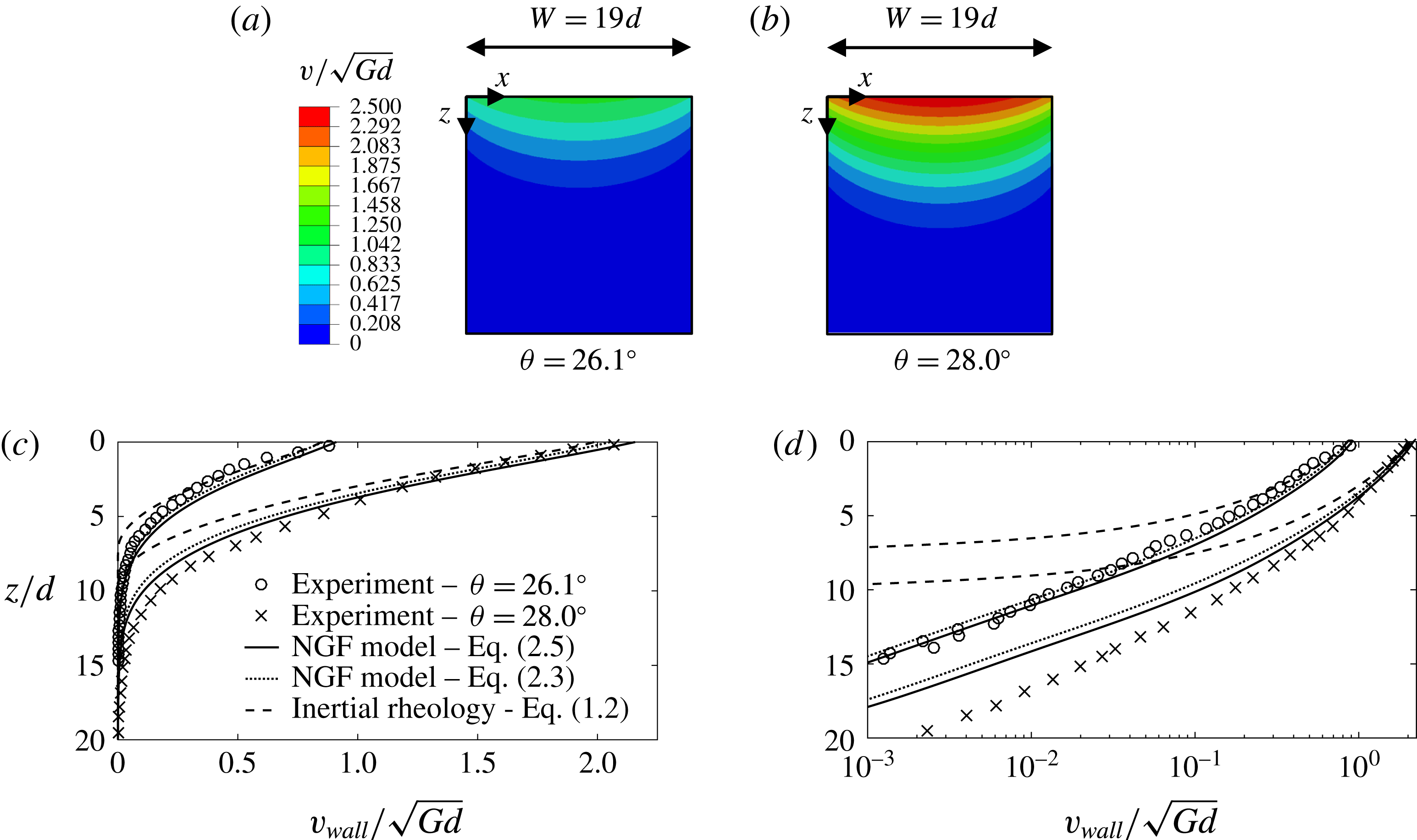
Flow fields in a narrow channel of width
 $W/d=19$
. Contour plots of the normalized, steady-state velocity field,
 $v/\sqrt{Gd}$
, in the
 $x$
–
 $z$
-plane for (a)
 $\unicode[STIX]{x1D703}=26.1^{\circ }$
and (b)
 $\unicode[STIX]{x1D703}=28.0^{\circ }$
calculated using the steady-state NGF model (2.5). Normalized velocity field at the wall,
 $v_{wall}/\sqrt{Gd}$
, as a function of the depth beneath the free surface,
 $z$
, for each surface inclination angle,
 $\unicode[STIX]{x1D703}$
, in (c) linear and (d) semi-logarithmic scale. Symbols represent the experimental data of Jop et al. (Reference Jop, Forterre and Pouliquen2007); solid lines are the calculated results of the steady-state NGF model (2.5); dotted lines are the calculated steady results of the dynamical NGF model (2.3); and dashed lines are the calculated results of the local inertial rheology (1.2).
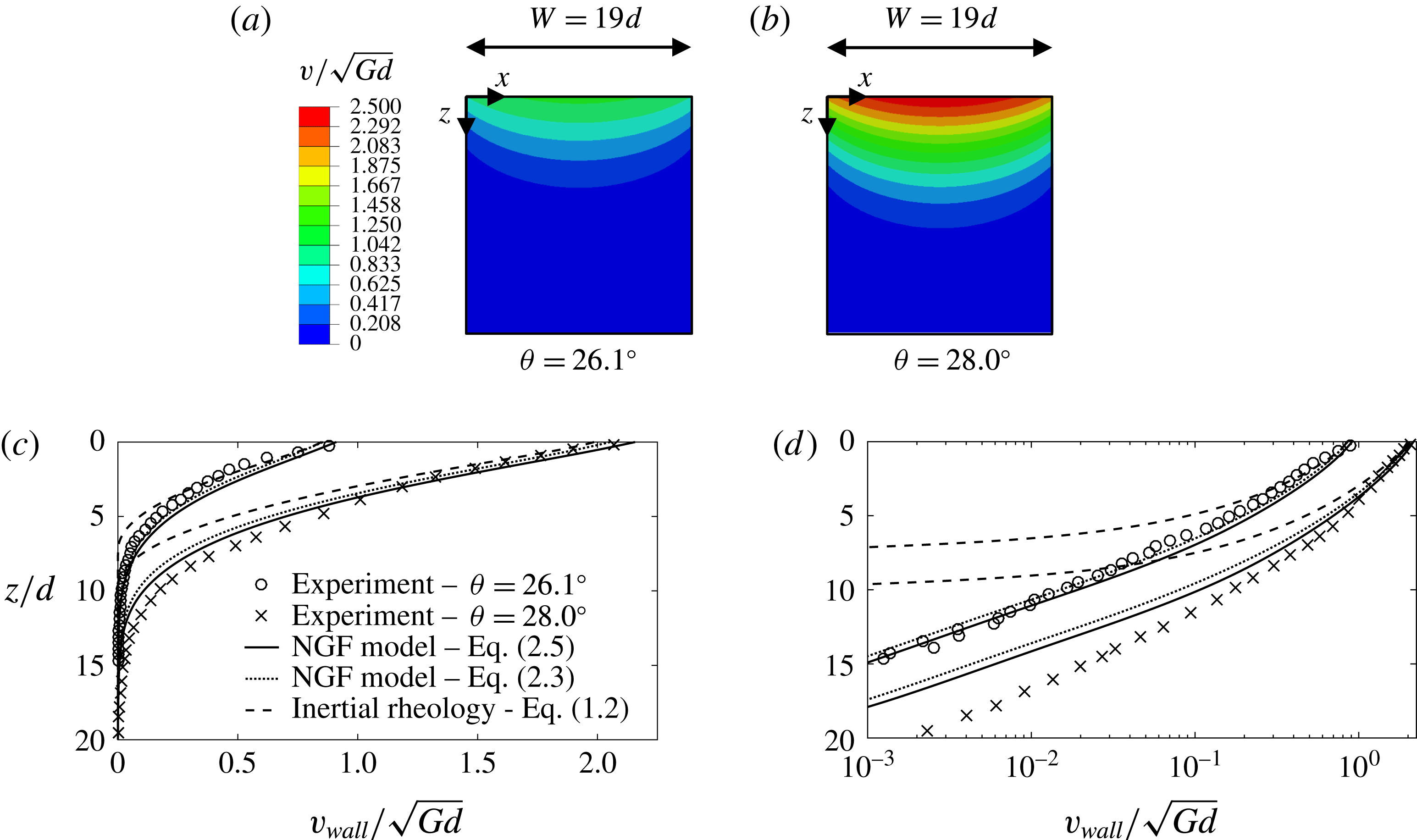
Following the experiments of Jop et al. (Reference Jop, Forterre and Pouliquen2007), we begin by considering narrow channels of width
 $W/d=19$
for two values of the free surface inclination angle –
 $\unicode[STIX]{x1D703}=26.1^{\circ }$
and
 $\unicode[STIX]{x1D703}=28.0^{\circ }$
– and calculate steady flow predictions using the steady-state form of the NGF model (2.5) and the computational set-up of figure 1(b). Contour plots of the normalized velocity field at steady state,
 $v/\sqrt{Gd}$
, in the
 $x$
–
 $z$
-plane for each case are shown in figure 2(a,b). As expected, flow is at its most rapid at the free surface with the velocity decaying into the bulk (in the
 $z$
-direction). In the cross-channel direction (the
 $x$
-direction), the velocity field has a clear bowed shape due to the frictional side walls. As is clear from the contour plots of figure 2(a,b), flow for the
 $\unicode[STIX]{x1D703}=28.0^{\circ }$
case is considerably more rapid. For the purpose of comparing to experiments, we introduce the wall velocity field,
 $v_{wall}(z)$
, at an
 $x$
-position of
 $x=d$
– one grain diameter inside the side wall. Figure 2(c) displays the good quantitative agreement between the simulated wall flow fields (solid lines) and the experimental data of Jop et al. (Reference Jop, Forterre and Pouliquen2007) (symbols) for the two inclination angles considered. In particular, the NGF model captures both the rapid flow near the free surface as well as the exponentially decaying, creeping velocity field deep beneath the surface – made clear in the semi-logarithmic-scale plot of the wall velocity field in figure 2(d).
For comparison, we have also calculated steady flow predictions of the dynamical form of the NGF model (2.3) in a narrow channel of width
 $W/d=19$
. To obtain steady flow predictions for the dynamical form of the NGF model, an initial condition for the fluidity field,
 $g$
, is required due to the presence of the time derivative in (2.3). Since steady (
 $t\gg t_{0}$
) solutions of the dynamical form of the NGF model (2.3) are expected to be similar to the solutions of the steady-state NGF model (2.5), we utilize the respective solutions of the steady-state form as the initial condition for the dynamical form for each case. Then, we choose an arbitrary value of the time scale
 $t_{0}$
and run the simulation to a final time of
 $1000t_{0}$
to ensure that the steady state is attained. The material parameters and boundary conditions remain unchanged. The calculated steady wall velocity fields for the dynamical form of the NGF model for the cases of
 $\unicode[STIX]{x1D703}=26.1^{\circ }$
and
 $\unicode[STIX]{x1D703}=28.0^{\circ }$
are included in figure 2(c,d) as dotted lines. For both free surface inclination angles, the calculated steady predictions of both forms of the NGF model are quite similar in both the rapidly flowing surface layer and the creeping bulk. Since solutions are much more easily obtained through the steady-state form of the NGF model (2.5), it is typically preferable to use this form in practice.
As a second comparison, we have calculated steady flow predictions of the local inertial rheology (1.2) in a narrow channel of width
 $W/d=19$
. Steady flow predictions of the local inertial rheology (1.2) are obtained by setting the non-local amplitude to zero, i.e.
 $A=0$
, and leaving all other material parameters and boundary conditions unchanged. The calculated wall velocity fields for the local inertial rheology for the cases of
 $\unicode[STIX]{x1D703}=26.1^{\circ }$
and
 $\unicode[STIX]{x1D703}=28.0^{\circ }$
are plotted in figure 2(c,d) as dashed lines. In the rapidly flowing surface layer, the NGF model and the local inertial rheology offer similar flow field predictions, which are both in agreement with experimental data. However, beneath the surface, the local inertial rheology predicts a sharp flow cutoff, clearly observed in the semi-logarithmic-scale plot of figure 2(d), whereas the NGF model is capable of capturing the exponentially decaying, creeping bulk. The NGF model clearly provides significantly improved predictions of steady, dense granular heap flow fields compared to the local inertial rheology.
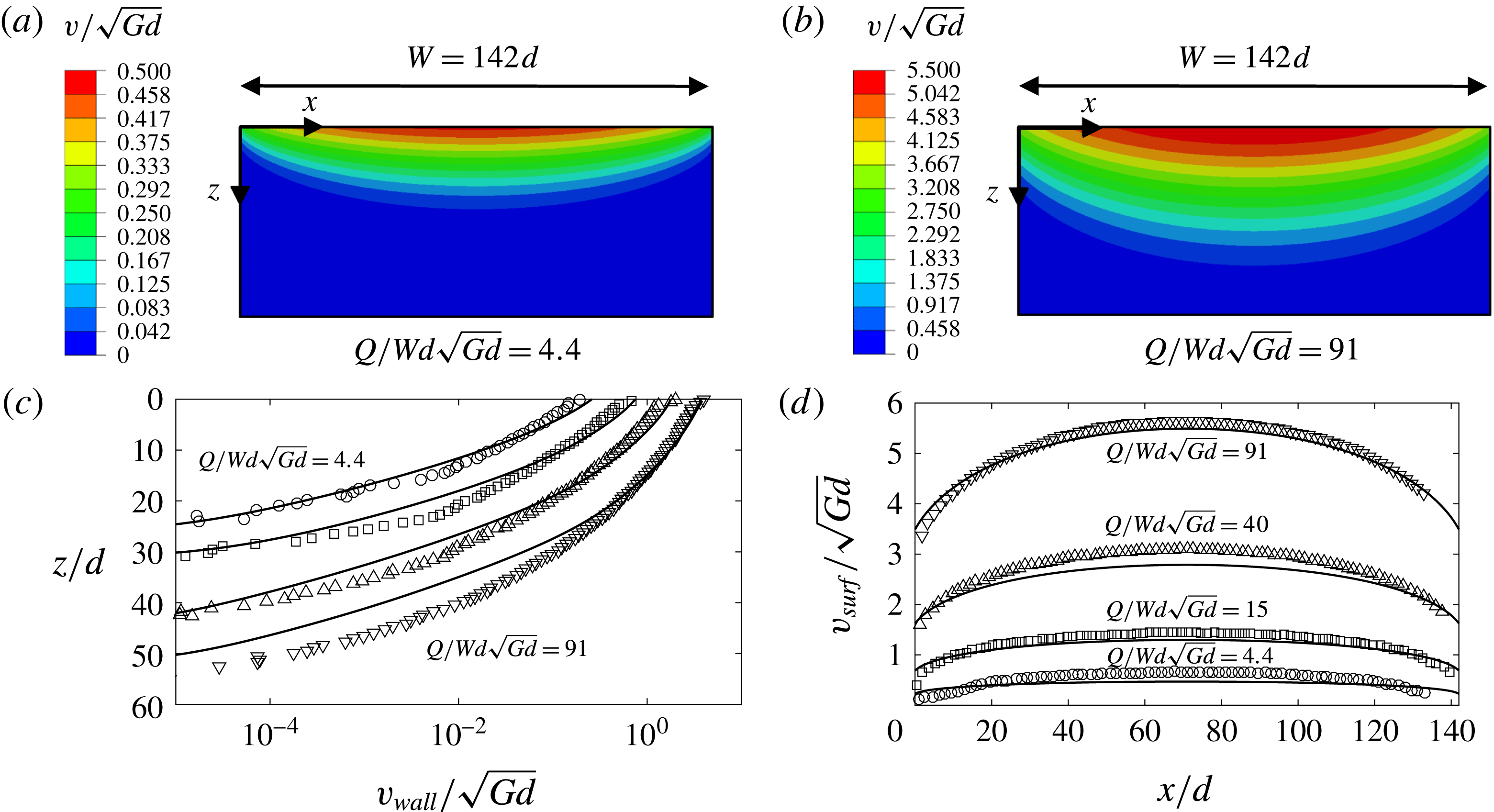
Flow fields in a wide channel of width
 $W/d=142$
. Contour plots of the normalized, steady-state velocity field,
 $v/\sqrt{Gd}$
, in the
 $x$
–
 $z$
-plane for (a)
 $Q/Wd\sqrt{Gd}=4.4$
and (b)
 $Q/Wd\sqrt{Gd}=91$
calculated using the NGF model. (c) Normalized velocity field at the wall,
 $v_{wall}/\sqrt{Gd}$
, as a function of the depth beneath the free surface,
 $z$
, and (d) normalized velocity field on the surface,
 $v_{surf}/\sqrt{Gd}$
, as a function of
 $x$
for each volume flow rate,
 $Q/Wd\sqrt{Gd}$
. Symbols represent the experimental data of Jop (Reference Jop2006) and solid lines are the calculated results of the steady-state NGF model.
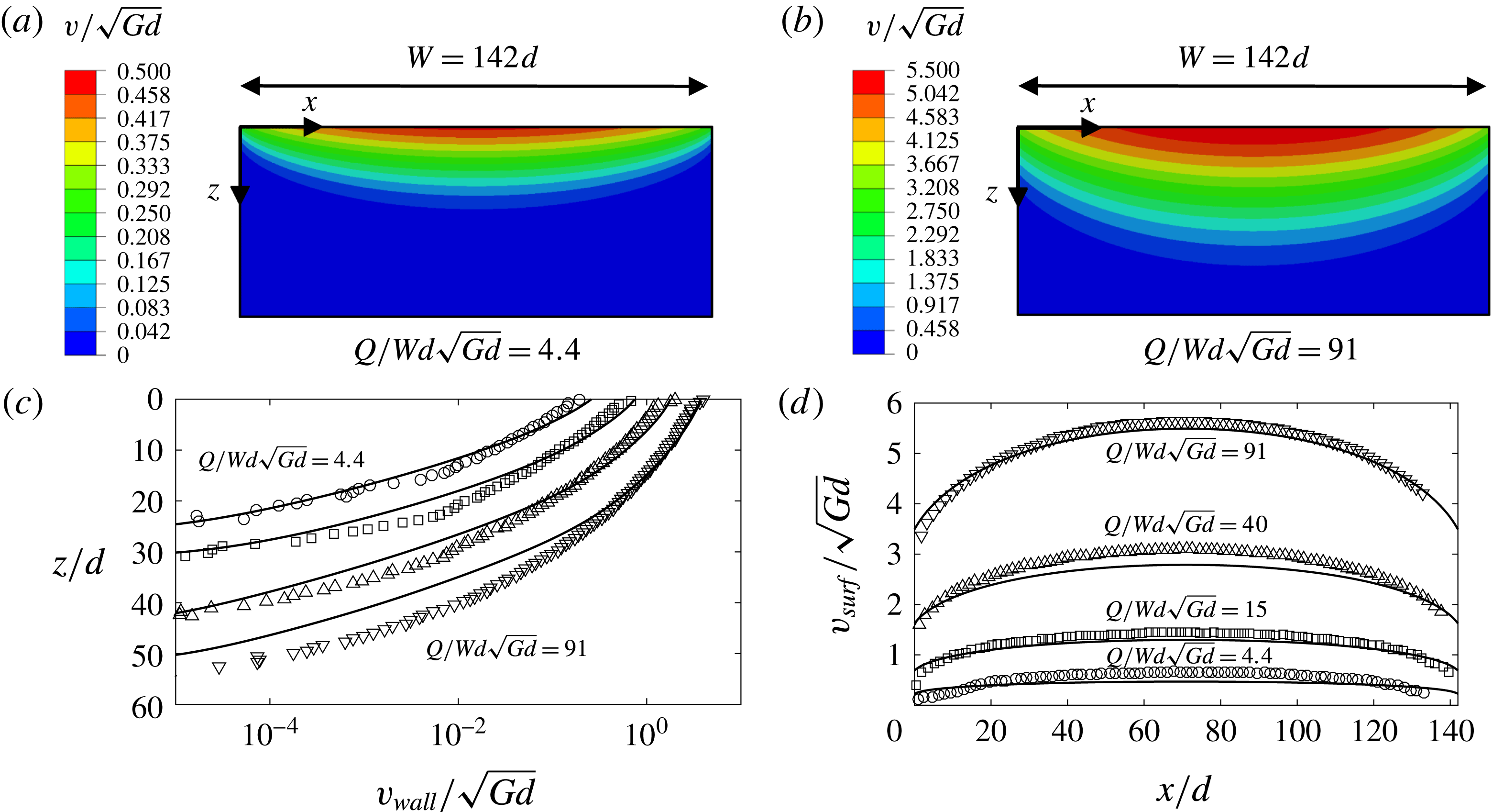
Next, returning to the steady-state NGF model (2.5), we consider a wider channel with
 $W/d=142$
and compare to the experimental data of Jop (Reference Jop2006). For this set of experiments, the flow rate,
 $Q/Wd\sqrt{Gd}$
, was reported rather than the inclination angle,
 $\unicode[STIX]{x1D703}$
. Accordingly, we consider flow rates of
 $Q/Wd\sqrt{Gd}=4.4,15,40$
and 91. (In our calculations, the inclination angle,
 $\unicode[STIX]{x1D703}$
, is prescribed, so for the
 $W/d=142$
simulations,
 $\unicode[STIX]{x1D703}$
is iteratively adjusted to achieve the desired volume flow rate. We utilize a channel depth of
 $H/d=140$
and a mesh resolution of
 $0.5d$
.) Contour plots of the normalized, steady-state velocity field,
 $v/\sqrt{Gd}$
, in the
 $x$
–
 $z$
-plane are shown in figure 3(a,b) for the least rapid and most rapid flow rates,
 $Q/Wd\sqrt{Gd}=4.4$
and 91, respectively. Again, we observe that the velocity decays with the depth beneath the surface and is greater in the centre of the channel than at the walls. In the contour plots, it is clear that the size of the rapidly flowing surface layer is larger for the higher flow rate. Figure 3(c) then shows the comparison of the calculated wall velocity field,
 $v_{wall}(z)$
, to the experimental data of Jop (Reference Jop2006) for all four volume flow rates, and again the quantitative agreement is good both for the rapid flow near the surface as well as the creeping bulk. Defining the surface flow field as
 $v_{surf}(x,z=0)$
, figure 3(d) shows that the calculated surface flow field is also in agreement with experiments – both at the wall and in the centre of the channel. Overall, the NGF model is able to capture the salient aspects of the flow fields in steady, dense granular heap flow over a range of channel widths.
3.3 Volume flow rate and maximum velocity
Additional insight may be obtained by comparing the predicted relationships between global quantities – such as the relationships between volume flow rate,
 $Q$
, maximum velocity,
 $v_{max}=v(x=W/2,z=0)$
and free surface inclination angle,
 $\unicode[STIX]{x1D703}$
– to experiments. Before making such comparisons, we first consider some consequences of dimensional analysis. The dense granular heap flow configuration of figure 1(a) relates the following quantities –
 $W$
,
 $d$
,
 $\unicode[STIX]{x1D70C}_{s}$
,
 $\unicode[STIX]{x1D70C}_{s}G$
and
 $\unicode[STIX]{x1D703}$
– to the consequent volume flow rate,
 $Q$
, and maximum velocity,
 $v_{max}$
. However, the analysis of Jop et al. (Reference Jop, Forterre and Pouliquen2005) showed that the scaling suggested by the local inertial rheology (1.1) could account for the observed scalings between
 $Q$
,
 $v_{max}$
and
 $\unicode[STIX]{x1D703}$
, and importantly, in the local inertial rheology, the grain size does not appear independently – instead combined with the grain material density as
 $\unicode[STIX]{x1D70C}_{s}d^{2}$
. Consequently, the reduced set of quantities –
 $W$
,
 $\unicode[STIX]{x1D70C}_{s}d^{2}$
,
 $\unicode[STIX]{x1D70C}_{s}G$
and
 $\unicode[STIX]{x1D703}$
– should give
 $Q$
and
 $v_{max}$
. Straightforward dimensional analysis leads to the conclusion that the local inertial rheology suggests a one-to-one relationship between the following three dimensionless quantities:
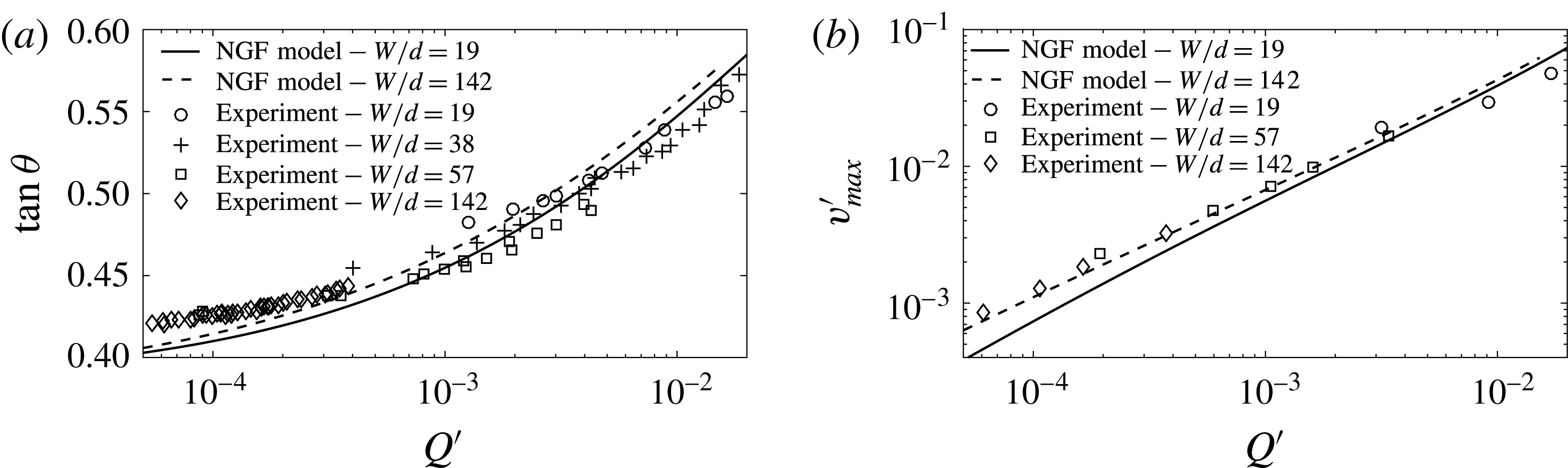
 $$\begin{eqnarray}\displaystyle Q^{\prime }=\frac{Qd}{G^{1/2}W^{7/2}},\quad v_{max}^{\prime }=\frac{v_{max}d}{G^{1/2}W^{3/2}},\quad \text{and}\quad \unicode[STIX]{x1D703}. & & \displaystyle\end{eqnarray}$$
Such a collapse was observed in experimental data by Jop et al. (Reference Jop, Forterre and Pouliquen2005), and their data in the form
 $\tan \unicode[STIX]{x1D703}$
versus
 $Q^{\prime }$
and
 $v_{max}^{\prime }$
versus
 $Q^{\prime }$
are reproduced in figure 4(a,b), respectively, for several channel widths. Also plotted in figure 4 are the respective calculated relationships obtained from the NGF model for
 $W/d=19$
and 142 – both a narrow and a wide channel. We note that the constant wall friction coefficient,
 $\unicode[STIX]{x1D707}_{wall}$
, was determined by fitting to the data of figure 4(a), rather than by fitting to individual flow fields of § 3.2. We observe first that agreement with experiments may be obtained as a result. Second, while the local inertial rheology predicts a perfect collapse between
 $Q^{\prime }$
,
 $v_{max}^{\prime }$
and
 $\unicode[STIX]{x1D703}$
, the collapse for the NGF model is approximate with the differences between the simulated relationships for the two channel widths being small, indicating that non-local effects – i.e. the presence of the creeping bulk – are secondary in these scaling relationships. Therefore, the NGF model is able to account for the most significant deficiency in the predictions of the local inertial rheology applied to steady, dense heap flow – i.e. the existence of the creeping bulk – while approximately maintaining its greatest success – i.e. the scalings between
 $Q^{\prime }$
,
 $v_{max}^{\prime }$
, and
 $\unicode[STIX]{x1D703}$
.
Relationships between (a) free surface inclination angle,
 $\unicode[STIX]{x1D703}$
, and dimensionless volume flow rate,
 $Q^{\prime }$
, and (b) dimensionless maximum velocity,
 $v_{max}^{\prime }$
, and dimensionless flow rate,
 $Q^{\prime }$
, for steady, dense granular heap flow. Symbols represent the experimental data of Jop et al. (Reference Jop, Forterre and Pouliquen2005) and lines are calculated predictions of the steady-state NGF model.

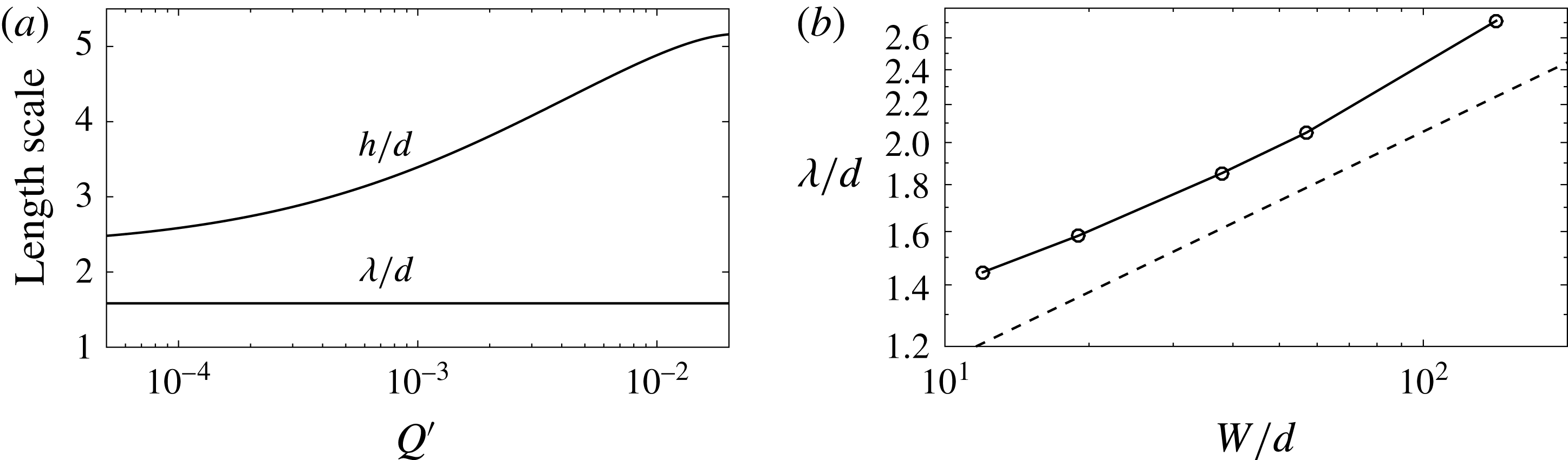
3.4 Two length scales
Finally, to explore the qualitative difference between the rapidly flowing surface layer and the creeping bulk, we introduce two characteristic length scales. Following Jop et al. (Reference Jop, Forterre and Pouliquen2007), the rapidly flowing surface layer is characterized by the mean flow depth,
 $h$
, defined as
 $h=Q/Wv_{max}$
. The creeping bulk is characterized by the decay length of the exponential tail in the mid-channel velocity field,
 $\unicode[STIX]{x1D706}$
, defined through
 $v(x=W/2,z)\sim \exp (-z/\unicode[STIX]{x1D706})$
for large
 $z$
. Figure 5(a) shows both
 $h/d$
and
 $\unicode[STIX]{x1D706}/d$
versus the dimensionless flow rate,
 $Q^{\prime }$
, for the calculated results of the NGF model for
 $W/d=19$
. Importantly,
 $h$
is flow-rate dependent while
 $\unicode[STIX]{x1D706}$
is flow-rate independent, which agrees both qualitatively and quantitatively with experiments (see figure 4(b) of Jop et al. (Reference Jop, Forterre and Pouliquen2007) in which
 $\unicode[STIX]{x1D706}/d$
extracted from the wall flow field is approximately 2 for
 $W/d=19$
). This observation may be understood mathematically as follows. In the rapidly flowing layer where
 $\unicode[STIX]{x1D707}>\unicode[STIX]{x1D707}_{s}$
, the local contribution to (2.5),
 $g_{loc}$
, dominates, introducing the rate dependence of the local rheology. Conversely, in the creeping bulk where
 $\unicode[STIX]{x1D707}<\unicode[STIX]{x1D707}_{s}$
,
 $g_{loc}=0$
, rendering (2.5) rate independent (Kamrin & Koval Reference Kamrin and Koval2012) and leading to the rate independence of
 $\unicode[STIX]{x1D706}$
. Regarding the dependence of the length scales
 $h$
and
 $\unicode[STIX]{x1D706}$
on the channel width
 $W$
, since
 $h$
is defined through
 $Q$
and
 $v_{max}$
, its scaling may be understood through the arguments of § 3.3; however, due to the rate independence of
 $\unicode[STIX]{x1D706}$
, we expect that
 $\unicode[STIX]{x1D706}/d$
will only depend upon
 $W/d$
(see figure 2(b) of Henann & Kamrin (Reference Henann and Kamrin2013) for the analogous relationship between a flow length scale and geometry in split-bottom flow). Figure 5(b) shows
 $\unicode[STIX]{x1D706}/d$
versus
 $W/d$
calculated by the NGF model for channel widths ranging from
 $W/d=12$
to 142. The observed relationship appears close to a 1/4 power law (plotted as a dashed line for reference); however, appropriate experimental data to verify this point have not been reported.
(a) Calculated dependence of the size of the flowing zone,
 $h/d$
, and the creeping zone decay length,
 $\unicode[STIX]{x1D706}/d$
, on the dimensionless volume flow rate,
 $Q^{\prime }$
, for
 $W/d=19$
. (b) Relationship between creeping zone decay length,
 $\unicode[STIX]{x1D706}/d$
, and the channel width,
 $W/d$
. The dashed line represents a
 $1/4$
power law included for reference.

4 Discussion and conclusion
In this work, we have shown that the NGF model is capable of capturing several important experimentally observed aspects of steady, dense granular heap flow, including (i) wall and surface flow fields for a range of channel widths; (ii) the relationships between volume flow rate, maximum velocity and surface inclination; and (iii) the rate-dependent thickness of the rapidly flowing surface layer and the rate-independent decay length of the exponentially decaying velocity field in the creeping bed. Importantly, the NGF model offers improved flow predictions over the local inertial rheology while involving only one new dimensionless material parameter, the non-local amplitude
 $A$
. In our previous work, we determined the value of
 $A$
for glass beads by applying the NGF model to slow boundary-driven flows (Henann & Kamrin Reference Henann and Kamrin2013), and in the present work, we have continued to use this numerical value and demonstrated that good agreement with experiments is maintained in the case of steady, dense granular heap flow.
There remain several avenues for improvement and refinement. A major idealization of our modelling work is treating the friction coefficient between the granular material and the side walls as constant – instead of dependent on the slip velocity and velocity fluctuation as shown by Artoni & Richard (Reference Artoni and Richard2015). The recent work of Zhang & Kamrin (Reference Zhang and Kamrin2017) relating the granular fluidity to the velocity fluctuation suggests a path forward on this point, in which the wall friction coefficient is taken to be dependent on both the slip velocity and the granular fluidity.
We have limited attention to the case of steady, well-developed flow. To apply the NGF model to transient, developing flows, the incorporation of additional physics is required. The work of Jop et al. (Reference Jop, Forterre and Pouliquen2007) showed that accounting for macroscopic inertia in conjunction with the local inertial rheology was sufficient to obtain a reasonable description of the approach to steady state in dense granular heap flow, quantified by the overall flow rate and free surface velocity as a function of time. Since the inertial rheology and the NGF model provide comparable predictions in the rapid flow regime, if macroscopic inertia effects are reintroduced to (3.3), we expect to obtain similar results with the NGF model. Transient effects are not solely due to macroscopic inertia. For example, Reynolds dilation during shear initiation induces transient variations in the flow resistance, which are commonly described using critical-state models (Schofield & Wroth Reference Schofield and Wroth1968) but which are not yet included in the NGF model. Further, Ries et al. (Reference Ries, Brendel and Wolf2016) recently reported an exponential-type transient during the initiation of dense simple shearing of spheres, and it is not yet known whether this transient may be captured using the time-dependent, dynamical form of the non-local rheology (2.3).
In closing, the ability of the NGF model to capture steady, dense granular heap flow in a channel is an encouraging indication that the model might successfully be applied to other types of surface flow, such as the flows that arise in rotating drums. The essential physics of steady, dense granular flow in a rotating drum is expected to be the same as that in channel flows (MiDi Reference MiDi2004), but the geometric complexity of the rotating drum configuration gives rise to additional characteristics in the flow field, such as the S-shape of the free surface. Applying the NGF model to steady, dense flows in a rotating drum will possibly require more elaborate numerical techniques than our finite-element-based approach, such as the material point method (Dunatunga & Kamrin Reference Dunatunga and Kamrin2015), and is a task which is left to future work.
Acknowledgements
Discussions with K. Kamrin are gratefully acknowledged. This work was supported by funds from NSF-CBET-1552556.