





1. Introduction
A long-standing effort in geophysical fluid dynamics has been to include parametrisations of unresolved (or subgrid-scale) effects into coarse-resolution numerical models. This approach has been pursued for a long time in oceanographic modelling (e.g. Redi Reference Redi1982), in atmospheric modelling (e.g. McFarlane Reference McFarlane1987) and in the planetary dynamo community (e.g. Matsui & Buffett Reference Matsui and Buffett2013). In this approach, accounting for topography and roughness appears to be fundamental. Topography can act as a source of energy dissipation, mixing and angular-momentum transfer, thereby influencing the dynamics of most geophysical flows. For example, sea-floor roughness can control the oceanic mesoscale variability by weakening the baroclinic instability (e.g. Lacasce et al. Reference Lacasce, Escartin, Chassignet and Xu2019), or interact with vortices (e.g. Gulliver & Radko Reference Gulliver and Radko2022; Rodrìguez Martìnez et al. Reference Rodrìguez Martìnez, Zavala Sansón and Cruz-Gómez2026). In addition, the interaction between wave motions and topography has also been investigated in stably stratified fluids, showing that internal gravity waves can play a fundamental role in oceanic and atmospheric flows (e.g. Wurtele et al. Reference Wurtele, Sharman and Datta1996; Staquet & Sommeria Reference Staquet and Sommeria2002; Caulfield Reference Caulfield2021; Legg Reference Legg2021). In this context, the radiation of gravito-inertial waves due to a single seamount has also been recently investigated (Le Dizès et al. Reference Le Dizès, Grisouard, Thual and Mercier2025). On the contrary, the fate of rotating flows with topography in well-mixed buried fluid layers (e.g. in convective planetary cores, or subsurface oceans of icy moons) remains poorly understood (e.g. Vidal et al. Reference Vidal, Noir, Cébron, Burmann, Monville, Giraud and Charles2024, and references therein). Notably, the scarcity of direct observational constraints may explain why topography-driven inertial waves have received less attention than their gravity counterparts. For instance, deep-Earth studies agree that the core–mantle boundary (CMB; i.e. the interface between the liquid core and the solid mantle) deviates significantly from a smooth spherical shape, but there is no consensus regarding the amplitude and distribution of this topography. Yet, since topography-driven waves can dissipate energy near the boundary and transfer angular momentum, they may leave observable geophysical imprints on planetary rotation (e.g. Buffett Reference Buffett2010) or magnetic field variations (e.g. Yoshida & Hamano Reference Yoshida and Hamano1993).
Inertial waves arise in rapidly rotating and incompressible fluids due to the restoring force of the Coriolis acceleration. In unbounded fluids, their anisotropic propagation is governed by the dispersion relation (e.g. Greenspan Reference Greenspan1968)
 \begin{equation} \omega ^2 \boldsymbol{k}^2 = (2 \boldsymbol{\varOmega } \boldsymbol{\cdot } \boldsymbol{k})^2, \end{equation}
where
 $\boldsymbol{\varOmega }$
is the background rotation rate,
 $|\omega | \leqslant 2|\varOmega |$
is the wave angular frequency and
 $\boldsymbol{k}$
is the wavevector for a plane-wave ansatz
 $\propto \exp (\mathrm{i} (\boldsymbol{k} \boldsymbol{\cdot } \boldsymbol{r} - \omega t))$
with the position vector
 $\boldsymbol{r}$
. Inertial-wave motions can be generated in the bulk by boundary forcings (e.g. Rieutord & Valdettaro Reference Rieutord and Valdettaro2010; Sauret et al. Reference Sauret, Cébron, Le Bars and Le Dizès2012; Lemasquerier et al. Reference Lemasquerier, Grannan, Vidal, Cébron, Favier, Le Bars and Aurnou2017), bulk turbulent flows such as rotating convection (e.g. Lin Reference Lin2021) or wave turbulence (e.g. Yarom & Sharon Reference Yarom and Sharon2014; Le Reun et al. Reference Le Reun, Favier, Barker and Le Bars2017; Monsalve et al. Reference Monsalve, Brunet, Gallet and Cortet2020), or by local forcings as in the classic experiment of Görtler (as reported in Greenspan (Reference Greenspan1968)). Topography provides another natural local forcing, exciting responses ranging from columnar structures at low frequencies
 $|\omega /\varOmega | \ll 1$
(e.g. Taylor Reference Taylor1921, Reference Taylor1922) to evanescent waves above the cutoff frequency
 $|\omega /\varOmega | \gtrsim 2$
(Nosan et al. Reference Nosan, Burmann, Davidson and Noir2021). Despite their importance, the mechanisms governing energy exchange between topography and inertial waves remain poorly understood.
In two-dimensional settings, previous works have laid some foundations. For instance, Johnson (Reference Johnson1982) derived the inertial-wave drag induced by a ridge, while Machicoane et al. (Reference Machicoane, Labarre, Voisin, Moisy and Cortet2018) later investigated the wake of a horizontally translating cylinder using both experiments and simulations. For gravito-inertial waves, Bell (Reference Bell1975) derived an asymptotic theory in the shallow regime characterised by
 $h_0 k \ll 1$
, where
 $h_0$
is the topographic height for a three-dimensional sinusoidal topography. We refer the reader to Legg (Reference Legg2021) for a modern account of the latter theory. Note that a similar approach has also been employed in geophysics including magnetic effects (e.g. Jault Reference Jault2020; Monville et al. Reference Monville, Cébron and Jault2025, and references therein). All these studies show the key role of the wave-driven component of the topographic drag, which is anticipated to prevail over diffusive effects under geophysical conditions.
However, the investigation of topographic stress remains an active field of research. For instance, Burmann & Noir (Reference Burmann and Noir2018) experimentally investigated the spin-up of a rotating fluid with a bottom chessboard-like topography. Using the measured spin-up time as a proxy for the torque, they identified an optimal wavelength for a given topographic height that maximises the torque (i.e. minimises the spin-up time). Velocimetry measurements also confirmed the key role of inertial waves generated by topography in their experiments. Yet, the scaling of this optimal wavelength remained an open question. Moreover, the proposed scaling laws for the pressure drag are yet to be confirmed through numerical simulations or laboratory experiments. Finally, to the best of our knowledge, there are also no predictive scaling laws for the drag produced by steady flows over finite-amplitude topography, that is, with finite-amplitude slopes
 $h_0 k \gtrsim 1$
.
In this study, we benchmark for the first time the proposed laws for shallow topographies using direct numerical simulations (DNS). These simulations are performed for a uniform background flow over three-dimensional sinusoidal topographies in a periodic domain. Moreover, we also introduce a novel asymptotic model that extends previous theoretical models for shallow topographies (e.g. Bell Reference Bell1975; Monville et al. Reference Monville, Cébron and Jault2025), to encompass fully three-dimensional steep topographies within the quasi-geostrophic (QG) regime of vanishingly small viscosity and nonlinearities. The paper is organised as follows. We introduce the mathematical and numerical models in § 2. Then, we present asymptotic theories in § 3, which allow us to obtain drag formulas for shallow and steep topographies. The asymptotic results are compared with the numerical simulations in § 4. A general discussion is given in § 5, in which we notably revisit previous experimental results in the light of the new steep model. Finally, we conclude the paper in § 6. Additional details about the calculations are given in Appendices A and B.
2. Formulation of the problem
2.1. Governing equations
We consider a homogeneous incompressible fluid, with constant density
 $\rho$
and kinematic viscosity
 $\nu$
. The fluid is subject to planetary rotation at angular velocity
 $\boldsymbol{\varOmega } = \varOmega \boldsymbol{1}_z$
along the unit vector
 $\boldsymbol{1}_z$
in a semi-infinite half-space. The fluid is bounded from below by a solid boundary, which is given by a regular egg-box topography defined as
 \begin{equation} h(x,y,k) = h_0 \sin (kx)\sin (ky), \end{equation}
where
 $h_0$
is the height of the topography and
 $k$
is its wavenumber in the two horizontal directions. The situation is illustrated in figure 1. In the frame rotating with
 $\varOmega$
, we decompose the velocity field as
 $\boldsymbol{U}_0 + \boldsymbol{u}$
, where
 $\boldsymbol{U}_0$
is a background uniform flow and
 $\boldsymbol{u}$
is a flow perturbation resulting from the interaction of
 $\boldsymbol{U}_0$
with the topography. For simplicity,
 $\boldsymbol{U}_0$
is assumed to be a spatially uniform and steady flow along the
 $x$
direction such that
 \begin{equation} \boldsymbol{U}_0 = U_0 \boldsymbol{1}_x. \end{equation}
In the rotating frame, the governing equations for
 $\boldsymbol{u}$
are then the incompressible Navier–Stokes equations given by
 \begin{equation} \partial _t \boldsymbol{u} + (\boldsymbol{U}_0 \boldsymbol{\cdot } \boldsymbol{\nabla }) \boldsymbol{u} + (\boldsymbol{u} \boldsymbol{\cdot } \boldsymbol{\nabla }) \boldsymbol{u} + 2\boldsymbol{\varOmega } \times \boldsymbol{u} = - \boldsymbol{\nabla }(p/\rho ) + \nu \boldsymbol{\nabla} ^2 \boldsymbol{u}, \quad \boldsymbol{\nabla }\boldsymbol{\cdot } \boldsymbol{u} = 0, \end{equation}
where
 $p$
is a generalised pressure (including centrifugal acceleration). Equations (2.3a
,
b
) are then supplemented with boundary conditions. The no-slip boundary condition at the bottom surface is given by
 \begin{equation} \left . ( \boldsymbol{u}+\boldsymbol{U}_0 ) \right |_{z=h} = \boldsymbol{0}. \end{equation}
It can be decomposed into tangential and normal components along the surface as
 \begin{equation} \left . \left (\boldsymbol{u} + \boldsymbol{U}_0 \right ) \boldsymbol{\cdot }\hat {\boldsymbol{n}}\right |_{z=h}=0, \quad \left . \left (\boldsymbol{u} + \boldsymbol{U}_0 \right ) \times \hat {\boldsymbol{n}}\right |_{z=h}=\boldsymbol{0}, \end{equation}
where we have introduced the unit normal vector
 $\hat {\boldsymbol{n}}$
given by
 \begin{equation} \hat {\boldsymbol{n}}=\frac {\left (-\partial _x h, -\partial _{\!y} h, 1\right )^\top }{\sqrt {1 + (\partial _x h)^2+(\partial _{\!y} h)^2}}. \end{equation}
The non-penetration condition in (2.5a ), which can be explicitly written as
 \begin{equation} u_z = (u_x+U_0) \partial _x h + u_{\!y} \partial _{\!y} h \quad \text{at } \quad z = h, \end{equation}
provides the relevant boundary condition for the inertial-wave excitation considered here. On the contrary, the tangential component in (2.5b ) drives a boundary-layer solution within a bottom Ekman layer (which can often be neglected for the pressure-drag estimate).
Unidirectional flow
 $\boldsymbol{U}_0 = U_0 \boldsymbol{1}_x$
past a periodic topography
 $h(x,y) = h_0 \sin {(k x)} \sin {(k y)}$
, with horizontal wavenumber
 $k$
and wavelength
 $\lambda =2\pi /k$
, over a square surface of area
 $L^2$
.

Our main concern in this study will be the value of the drag exerted on the topography by the background flow. Hence, we define the pressure force per unit of surface acting on the topography as (e.g. Monville et al. Reference Monville, Cébron and Jault2025)
 \begin{equation} \boldsymbol{F}_{\!p} = \frac {1}{L^2}\iint p|_{z=h} \, \hat {\boldsymbol{n}} \, \mathrm{d}S, \quad \mathrm{d}S = \sqrt {1 + (\partial _x h)^2 + (\partial _{\!y} h)^2} \, \mathrm{d} x \,\mathrm{d} y, \end{equation}
where the force is normalised (by convention) by the area of the projected square surface of side length
 $L$
. Finally, the topography-driven drag in the direction of the flow is given by
 $\boldsymbol{F}_{\!p} \boldsymbol{\cdot } \boldsymbol{1}_x = -D$
with
 \begin{equation} D = \frac {1}{L^2} \iint p|_{z=h} \, \partial _x h \, \mathrm{d}x \, \mathrm{d}y, \end{equation}
where
 $D$
is the pressure drag per unit of surface.
2.2. Dimensionless parameters
As usual in geophysical fluid dynamics, it is worth introducing dimensionless numbers to discuss the various possible dynamical regimes. To do so, we define a topographic Ekman number as
 \begin{equation} E_{\lambda } = \frac {\nu k^2}{\varOmega }, \end{equation}
which characterises the ratio of viscous to Coriolis forces at the scale of the topography, and the usual Ekman number defined as
 \begin{equation} E_{L} = \frac {\nu }{\varOmega L^2} \end{equation}
that will be used in the numerical simulations in a finite domain of size
 $L$
. We also introduce a local Rossby number given by
 \begin{equation} \textit{Ro} = \frac {u k}{\varOmega }, \end{equation}
where
 $u$
is a typical amplitude of the perturbed flow
 $\boldsymbol{u}$
. It represents the relative strength of the nonlinear term to Coriolis force at the scale of the topography in (2.3a
). In this study, we will consider waves emitted by the topography in the small-amplitude regime
 $u \ll U_0$
, because this regime is amenable to simulations and asymptotic analysis. Using typical estimates for the Earth’s core, namely
 $\varOmega \approx 7.3 \times 10^{-5}$
rad s
 ${}^{-1}$
for the planetary rotation,
 $U_0 \sim 10^{-4} {-} 10^{-3}$
m s
 ${}^{-1}$
for a core-flow amplitude (e.g. Jault Reference Jault2020; Buffett Reference Buffett2021) and
 $k \sim 10^{-3}{-}10^{-1}$
km
 ${}^{-1}$
for small-scale topography at the CMB (e.g. figure 1(b) in Vidal et al. (Reference Vidal, Noir, Cébron, Burmann, Monville, Giraud and Charles2024)), we obtain values of the local Rossby number
 $Ro \ll 1$
and of the local Ekman number
 $E_{\lambda }\lesssim 10^{-9}$
. Therefore, we focus on low-
 $Ro$
regimes in the following. This will greatly simplify the equations in the asymptotic theory, as presented in § 3.
2.3. Numerical modelling
In addition to asymptotic calculations, we perform DNS. To do so, we employ the open-source code Nek5000 (e.g. Fischer Reference Fischer1997; Fischer et al. Reference Fischer, Loth, Lee, Lee, Smith and Bassiouny2007). This is a high-order spectral-element code, which can solve the incompressible Navier–Stokes equations in complex geometries. This code has been well validated for the simulation of turbulent flows of geophysical interest, such as mechanically driven flows in ellipsoids (e.g. Favier et al. Reference Favier, Grannan, Le Bars and Aurnou2015; Cébron et al. Reference Cébron, Vidal, Schaeffer, Borderies and Sauret2021) or turbulent convection with topography (e.g. Oliver et al. Reference Oliver, Blackman, Tarduno and Calkins2025; Secchi et al. Reference Secchi, Gatti, Piomelli and Frohnapfel2025). Temporal discretisation is accomplished by a third-order semi-implicit formulation, in which the nonlinear and rotation terms are treated explicitly in time and all remaining linear terms are treated implicitly. Note that our solution is dealiased following the
 $3/2$
rule for an exact quadrature of the nonlinear terms.
Here, the computational domain with a bottom topography is obtained from a Cartesian box of size
 $L_x \times L_{\!y} \times H$
, whose horizontal lengths are
 $L_x = L_{\!y} = L$
and its vertical height is
 $H = 3 L$
. This Cartesian mesh is made of
 $\mathcal{E} = 2550$
non-overlapping hexahedral elements. Inside each element, the unknown velocity is represented as the tensor-product Lagrange polynomials of order
 $\mathcal{N}=9{-}19$
based at the Gauss–Lobatto–Legendre (respectively order
 $\mathcal{N} - 2$
at Gauss–Legendre points for the pressure), which corresponds to a number of degrees of freedom for each velocity component scaling as
 $\mathcal{N}^3 \mathcal{E}$
. The mesh is refined near the top and bottom boundaries, such that the element height at these boundaries is comparable to the Ekman boundary-layer thickness
 $\sqrt {\nu /\varOmega }$
. This refinement ensures that the Ekman boundary layer is resolved by approximately
 $9$
points. The bottom topography is imposed by vertically distorting the original Cartesian mesh in the
 $z$
direction. The new vertical coordinates
 $z_{\textit{new}}$
are expressed as a function of the old ones
 $z$
using the linear mapping given by
 \begin{equation} z_{\textit{new}}(x,y,z) = z + h(x,y) \left ( 1 - \frac {z}{H} \right )\!, \quad k = \iota \frac {2 \pi }{L} \quad (\iota \in \mathbb{N}^*), \end{equation}
such that
 $z_{\textit{new}}(x,y,0)=h(x,y)$
and
 $z_{\textit{new}}(x,y,H) = H$
. In practice, we have chosen
 $\iota =3$
in most simulations. In this computational domain, we solve (2.3a
,
b
) together with no-slip condition (2.4) on the bottom boundary, and we enforce stress-free conditions at the top surface given by
 \begin{equation} \left . u_z \right |_{z=H} = 0, \quad \left . \partial _z u_{\!y} \right |_{z=H} = 0, \quad \left . \partial _z u_x \right |_{z=H} = 0. \end{equation}
In addition, periodic boundary conditions are imposed on the lateral walls.
The equations are solved in non-dimensional form using the length scale
 $L$
and the time scale
 $\varOmega ^{-1}$
, yielding values of
 $E_{L}$
varying between
 $10^{-6}$
and
 $3\times 10^{-3}$
. Given the Ekman number defined in (2.10), values between
 $E_{\lambda } = 3.6 \times 10^{-4}$
and
 $E_{\lambda } = 1.06$
are considered in the simulations. Moreover, the (dimensionless) intrinsic frequency
 $\omega _i/\varOmega = U_0k/\varOmega$
and the maximal slope
 $h_0 k$
are varied over the respective ranges of
 $[2 \times 10^{-4}, 4]$
and
 $[10^{-2}, 20]$
, as summarised in figure 2. Defining a local Reynolds number as
 $Re = Ro/E_{\lambda }$
, we obtain
 $Re \leqslant 1$
in the geostrophic cases and
 $Re \approx 250$
for the highest value. All the simulations remained stable and laminar. The simulations are initialised with a zero perturbation field, and are run until a steady-state solution is consistently achieved for all tested parameters. Only the cases with
 $\omega _i/\varOmega \gt 2$
present a non-steady behaviour. For other cases, the typical time required to reach this steady state is of the order of
 $E_{\lambda }^{-1}\varOmega ^{-1}$
, which corresponds to the damping time scale of inertial waves by viscosity in the bulk.
Survey of the parameter space
 $(\omega _i/\varOmega ,h_0k)$
in the DNS. Insets illustrate typical pressure variations in vertical cross-sections taken at
 $y = \pi /(2k)$
.

Finally, we point out that inertial waves are confined within a finite volume, contrary to the semi-infinite half-space model considered in the theoretical derivations. While the periodic boundary conditions prevent reflections from the lateral walls, wave motions can potentially be reflected on the upper stress-free boundary back in the interior, possibly interacting again with the topography to generate a secondary drag. To mitigate this undesirable effect, we stop the simulations before the arrival of the second reflection on the bottom topography.
3. Asymptotic models of the pressure drag produced by inertial waves
Our aim is to obtain theoretical predictions for wave-driven pressure drag, which will be compared with numerical simulations in § 4. Both
 $\boldsymbol{U}_0$
and the topography are steady in the rotating frame, such that
 $\boldsymbol{u}$
is expected to remain time-independent in the limit
 $Ro \ll 1$
if no instabilities or turbulence occur (requiring low enough values of the local Reynolds number
 $Re_{\lambda }\ll 1$
). Under these conditions, we simplify (2.3a
,
b
) and seek steady solutions of the linearised equations given by
 \begin{equation} (\boldsymbol{U}_0 \boldsymbol{\cdot } \boldsymbol{\nabla }) \boldsymbol{u} + 2\boldsymbol{\varOmega } \times \boldsymbol{u} = - \frac {1}{\rho }\boldsymbol{\nabla }\!p + \nu \boldsymbol{\nabla} ^2 \boldsymbol{u}, \quad \boldsymbol{\nabla }\boldsymbol{\cdot } \boldsymbol{u} = 0. \end{equation}
We present below asymptotic calculations for shallow topographies (
 $h_0 k \ll 1$
) and then for steep ones (
 $h_0 k \sim 1$
).
3.1. Inertial-wave drag for a shallow topography (
 $h_0 k \ll 1$
)

First, we consider the case of a topography with small slopes (
 $h_0 k\ll 1$
), hereafter referred to as ’shallow topography’. Following Bell (Reference Bell1975) and Legg (Reference Legg2021), non-penetration boundary condition (2.7) can be linearised in this asymptotic limit as
 \begin{equation} u_z (x,y,0) = \left . U_0 \partial _x h \right |_{z=0}, \end{equation}
which yields
 \begin{equation} u_z(x,y,0) = h_0 k U_0 \cos (kx)\sin (ky). \end{equation}
Thus,
 $u$
is of the order of
 $\mathcal{O}(h_0k U_0)\ll U_0$
for a shallow topography. Furthermore, the boundary condition suggests that the general solution of linearised equations (3.1a
,
b
) is in the form of a superposition of stationary plane waves with the same horizontal wavelength as the topography, such that
 \begin{equation} [\boldsymbol{u}, p] (x,y,z) = \sum _{m,n\in \{-1,1\}} [\boldsymbol{u}_{m,n}, p_{m,n}] \mathrm{e}^{\mathrm{i}( m k x + n k y -k_z z)}. \end{equation}
The vertical wavenumber
 $k_z$
is a priori a function of the sign coefficients
 $(m,n)$
, but we will drop the indices below for the sake of concision. We show in Appendix A that the solvability condition of the linear system yields the dispersion relation given by
 \begin{equation} \left [ m\left (\frac {\omega _i}{\varOmega }\right )-\mathrm{i}\left (\frac {\nu }{\varOmega }\right )(2k^2+k_z^2) \right ]^2 = \frac {4 k_z^2}{2k^2+k_z^2}, \end{equation}
where
 $\omega _i = U_0k$
is the intrinsic frequency. Using definition (2.10) for the Ekman number
 $E_{\lambda }$
, this relation can be rewritten as
 \begin{equation} \left [ m\frac {\omega _i}{\varOmega }-\mathrm{i} E_{\lambda }\left (2+\frac {k_z^2}{k^2}\right ) \right ] ^2 = \frac {4 k_z^2}{2k^2+k_z^2}. \end{equation}
We could consider two limits for this dispersion relation, depending on the relative magnitude of
 $E_{\lambda }$
and of the dimensionless intrinsic frequency
 $\omega _i/\varOmega$
. For
 $E_{\lambda } \ll \omega _i/\varOmega \leqslant 2$
the flow is in the form of inviscid inertial waves, whereas the flow is in the form of strongly attenuated wave motions for
 $\omega _i/\varOmega \ll E_{\lambda }$
. The typical pressure fields in the two regimes are illustrated in figure 3. In the following, we focus on the inviscid inertial-wave regime
 $E_{\lambda } \ll \omega _i/\varOmega \leqslant 2$
, as it is the most geophysically relevant limit.
Vertical cross-section of the pressure field for three different cases of low-Ekman-number inertial waves. The cross-section is taken at
 $y = \pi /(2k)$
where the amplitude of the topography is maximal.

In this inviscid inertial-wave regime, we can neglect the viscous term in (3.6), which yields the classical dispersion relation for inertial waves given by (A11) in Appendix A. The solution for
 $k_z$
is then given by
 \begin{equation} k_z^2 = 2m^2k^2\omega _i^2\big ( 4\varOmega ^2-\omega _i^2\big)^{-1}. \end{equation}
One of the two solutions corresponds to inertial waves tilted in the downstream direction of the background flow, which is consistent with the advection of the phase fields. The opposite sign would lead to waves tilted in the upstream direction relative to the mean flow, which are not physically relevant here. Using standing-wave ansatz (3.4) and (3.7), the vertical velocity is obtained from boundary condition (3.3) as
 \begin{equation} u_z(x,y,z) = h_0\omega _i\cos (kx-|k_z|z)\sin (ky), \quad |k_z| = \sqrt {2}k\omega _i\big( 4\varOmega ^2-\omega _i^2\big)^{-1/2}. \end{equation}
Next, we project (3.1a
) onto the
 $z$
axis, which gives in the inviscid regime
 \begin{equation} \mathrm{i}\rho m\omega _iu_z=-\mathrm{i}k_{z} p. \end{equation}
Substituting (3.8a , b ) into (3.9), the pressure is given by
 \begin{equation} p(x,y,z) = \rho \frac {h_0}{\sqrt {2}k}\omega _i\sqrt {4\varOmega ^2-\omega _i^2}\cos {(kx-|k_{z}|z)}\sin (ky). \end{equation}
The pressure drag per unit of surface then follows from (2.9). In the small-slope limit, the leading-order contribution for the pressure term is obtained at
 $z=0$
, yielding
 \begin{equation} D = \frac {1}{L^2}\iint p(z = 0) \, \partial _x h \, \mathrm{d}x \, \mathrm{d}y. \end{equation}
Substituting (3.10) into (3.11) then gives
 \begin{equation} D = \rho \frac {h_0^2}{\sqrt {2}L^2}\omega _i \sqrt {4\varOmega ^2-\omega _i^2} \iint \cos ^2(k x) \sin ^2{(k y)} \, \mathrm{d}x \, \mathrm{d}y. \end{equation}
Finally, considering a box of integration with dimensions
 $L \times L$
and with an integer number of wavelengths in both directions, the surface integration leads to
 \begin{equation} D = \rho \frac {h_0^2}{4\sqrt {2}}\omega _i \sqrt {4\varOmega ^2 - \omega _i^2} = D_0 g(\omega _i) \end{equation}
with
 \begin{equation} D_0 = \rho \frac {h_0^2}{2\sqrt {2}}\varOmega \omega _i, \quad g(\omega _i) = \sqrt {1 - \frac {\omega _i^2}{4\varOmega ^2}}, \end{equation}
where
 $D_0$
is the drag for shallow topography in the geostrophic limit and
 $g(\omega _i)$
is the correction that accounts for the non-geostrophic nature of waves at finite
 $\omega _i$
. We recover from (3.14) the classical drag formula for shallow topography given in Bell (Reference Bell1975) for a homogeneous fluid (see also (18) in Monville et al. (Reference Monville, Cébron and Jault2025)). As expected, the wave drag vanishes for
 $\omega _i = 2\varOmega$
, above which inertial waves do not propagate. The limit
 $\omega _i = 0$
corresponds to either a flat topography or a vanishing background flow, hence yielding a vanishing pressure drag in both situations.
3.2. Quasi-geostrophic inertial-wave drag for steep topography (
$h_0 k \sim 1$
)

The case with finite slopes
 $h_0 k \sim 1$
is more complicated, as there is no general analytical solution. In this case, the linearised non-penetration condition is no longer valid, and the perturbation amplitude
 $u$
is not necessarily smaller than
 $U_0$
. This implies that the Rossby number, defined in (2.12), is of the same order as the dimensionless intrinsic frequency
 $\omega _i/\varOmega = U_0k/\varOmega$
. Thus, we can no longer linearise the problem by self-consistently neglecting the nonlinear term
 $(\boldsymbol{u} \boldsymbol{\cdot } \boldsymbol{\nabla }) \boldsymbol{u}$
for the perturbation without neglecting the advective term
 $(\boldsymbol{U}_0 \boldsymbol{\cdot } \boldsymbol{\nabla }) \boldsymbol{u}$
. By restricting our analysis to the QG limit
 $\omega _i/\varOmega \ll 1$
, we can neglect both advection terms in (3.1a
). The momentum equation being dominated by a geostrophic balance at leading order in this limit, we expect vertical variations over the height
 $h_0$
of the topography to remain small. This allows us to keep the evaluation of the boundary condition fixed at
 $z=0$
. It follows that non-penetration condition (2.7) can be approximated for finite slopes as
 \begin{equation} u_z(x,y,0) = (u_x+U_0) \partial _x h + u_{\!y} \partial _{\!y} h \quad \text{at } \quad z = 0. \end{equation}
The above boundary condition again suggests a decomposition into stationary plane waves. However, we here expect multiple wavenumbers arising from the coupling between the perturbation and the topography. Hence, the standing-wave ansatz is written as
 \begin{equation} \left [ \boldsymbol{u}, p\right ] (x,y,z) = \sum _{m=-\infty }^{+\infty } \sum _{n=-\infty }^{+\infty } \left [ \boldsymbol{u}_{m,n}, p_{m,n} \right ] \mathrm{e}^{\mathrm{i} (mkx+nky+k_{z,m,n}z)}. \end{equation}
However, with this ansatz, the QG assumption is only valid for certain values of
 $m$
and
 $n$
, specifically when
 $(m^2+n^2)E_{\lambda } \ll 1$
. Therefore, we truncate expansion (3.16) to a maximum degree
 $M \lt E_{\lambda }^{-1/2}$
. Using numerical calculations, we show that this hypothesis is well justified for finite topographic wavenumbers. The QG balance yields
 \begin{align} u_x(x,y,z) &= \frac {k}{\rho \varOmega } \sum _{m=-M}^{M} \sum _{n=-M}^{M} -\frac {\mathrm{i}n}{2} p_{m,n} \mathrm{e}^{\mathrm{i} (mkx+nky+k_{z,m,n}z)}, \end{align}
 \begin{align} u_{\!y}(x,y,z) &= \frac {k}{\rho \varOmega } \sum _{m=-M}^{M} \sum _{n=-M}^{M} \frac {\mathrm{i}m}{2} p_{m,n} \mathrm{e}^{\mathrm{i} (mkx+nky+k_{z,m,n}z)}, \end{align}
 \begin{align} u_z(x,y,z) &= \frac {k}{\rho \varOmega } \sum _{m=-M}^{M} \sum _{n=-M}^{M} \frac {\sqrt {m^2+n^2}}{2} p_{m,n} \mathrm{e}^{\mathrm{i} (mkx+nky+k_{z,m,n}z)}. \end{align}
In the above equations,
 $k_{z,m,n} = \mathrm{i}E_{\lambda }k(m^2+n^2)^{3/2}/2$
represents the vertical wavenumber, which is the viscous damping term associated with the horizontal wavenumber
 $\boldsymbol{k} = (mk, nk, 0)^\top$
. Injecting (3.17a
–
c
) into boundary condition (3.15) yields the following recurrence relation:
 \begin{align} p_{m,n} \sqrt {m^2+n^2} & = \frac {h_0 k}{4} (n+m) (p_{m+1,n-1}-p_{m-1,n+1}) \nonumber \\ & + \frac { h_0 k}{4} (n-m) (p_{m-1,n-1} -p_{m+1,n+1}) \nonumber \\& + \frac {\mathrm{i} h_0 \rho \varOmega }{2} (\delta _{m,1} \delta _{n,-1} - \delta _{m,-1} \delta _{n,1} - \delta _{m,1} \delta _{n,1} + \delta _{m,-1} \delta _{n,-1}) U_0, \end{align}
where
 $\delta _{i,j}$
is the Kronecker delta function.
We show in Appendix A that (3.18) can be rewritten as a matrix inversion problem, giving us a unique solution for all pressure coefficients. Then, the wave-driven drag can be determined using (3.11) as
 \begin{align} D &= \frac {1}{L^2} \iint p(z = 0)\, \partial _x h \, \mathrm{d} x \,\mathrm{d} y \nonumber \\ &= \frac {\mathrm{i} h_0 k}{4L^2} \iint \sum _{m=-M}^{M} \sum _{n=-M}^{M} \Bigl [ p_{m,n} \mathrm{e}^{\mathrm{i}k(mx+ny)} \nonumber \\ &\quad \bigl ( \mathrm{e}^{\mathrm{i} k(x - y)} - \mathrm{e}^{\mathrm{i}k(-x + y)} - \mathrm{e}^{\mathrm{i}k(x + y)} + \mathrm{e}^{\mathrm{i}k(-x - y)} \bigr ) \Bigr ] \, \mathrm{d} x \,\mathrm{d} y. \end{align}
Because we integrate over an integer number of wavelengths in both directions, all the terms with a non-zero exponential argument will result in a zero value. Only the orders
 $m = \pm 1$
and
 $n = \pm 1$
will thus contribute to the integral, such that the drag expression reduces to
 \begin{eqnarray} D & = & \frac {\mathrm{i}h_0k}{4L^2}\iint \left ( p_{-1,1}- p_{1,-1} - p_{-1,-1} + p_{1,1} \right ) \, \mathrm{d} x \,\mathrm{d} y \nonumber \\ & = & \frac {\mathrm{i}h_0 k}{4} (p_{-1,1} - p_{1,-1} + p_{1,1} - p_{-1,-1}). \end{eqnarray}
Although the calculated drag only depends on
 $\{p_{\pm 1, \pm 1}\}$
, calculating higher-order terms is still necessary to achieve a good numerical convergence of the drag value. Finally, the mathematical expression of the pressure coefficients given in Appendix A suggests we can rewrite the steep QG drag as
 \begin{equation} D= D_0 f(h_0k), \end{equation}
where
 $D_0$
is given by (3.14a
) and
 $f(h_0k)$
is a geometrical correction (to be obtained numerically). In practice, we first calculate
 $D$
numerically and then compute
 $f(h_0k)=D/D_0$
. By definition, we have
 $f(0)=1$
since
 $D \to D_0$
when
 $h_0k \to 0$
.
4. Numerical results
4.1. Inertial-wave drag for a shallow topography
We first examine the drag coefficient in the limit of a shallow topography (
 $h_0 k \ll 1$
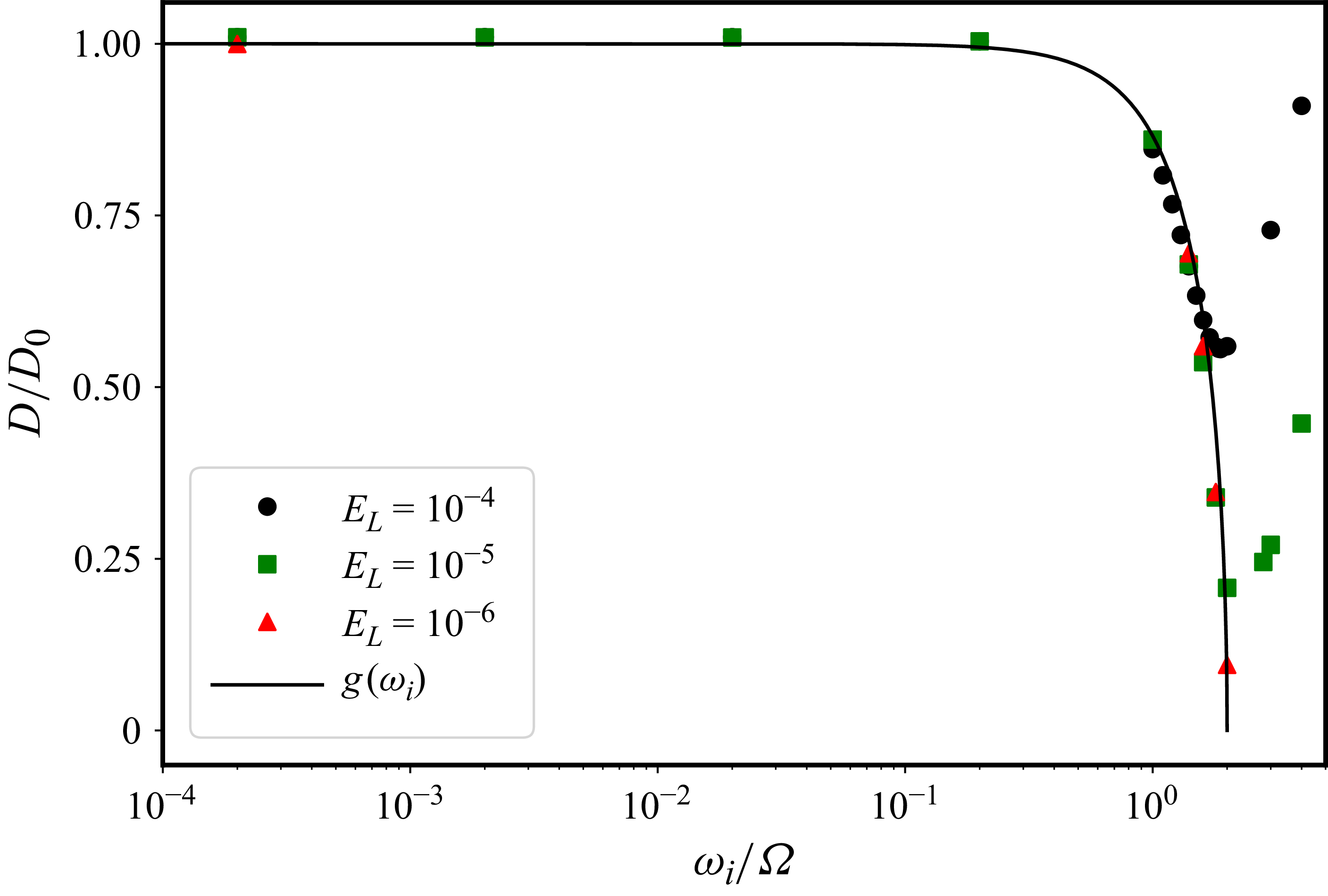
), as a function of the intrinsic frequency. We have shown that, in the limit of shallow topography, the wave drag
 $D$
can be expressed as in (3.13). We compare in figure 4 the value of the normalised drag
 $D/D_0$
as function of
 $\omega _i/\varOmega$
, in both the simulations at different values of
 $E_{L}$
and the asymptotic shallow theory. We have chosen
 $h_0/L = 5.3 \times 10^{-3}$
and
 $kL =6\pi$
(i.e.
 $h_0k=0.1$
), and we vary the background
 $U_0$
to scan in frequencies
 $\omega _i/\varOmega$
from
 $2\times 10^{-4}$
to
 $4$
. We observe a very good agreement between the numerical simulations and the shallow model predictions of
 $D=D_0$
from (3.14a
). We observe an abrupt decay past the critical value
 $\omega _i/\varOmega = \sqrt {2}$
, for which the theory predicts a maximum of the pressure. Beyond this maximum, the tilt of the inertial waves increases. We also report a critical value of the intrinsic frequency above which the numerical simulations depart significantly from the inviscid predictions. For instance, at
 $E_{L}=10^{-4}$
, this occurs at
 $\omega _i/\varOmega \sim 1.5$
, where the drag increases while we predict a continuing decay down to zero at
 $\omega _i=2\varOmega$
. This behaviour is due to the moderate Ekman number achievable in the simulations. The effect of a finite viscosity is further discussed in Appendices A and B. To illustrate the finite-viscosity nature of the discrepancy, we have carried out a limited number of simulations at lower values of the Ekman number
 $E_{L} = 10^{-4} {-} 10^{-6}$
. We observe that the divergence from the inviscid theory occurs closer to
 $\omega _i/\varOmega =2$
as the Ekman number gets smaller.
Normalised drag
 $D/D_0$
as a function of intrinsic frequency
 $\omega _i/\varOmega$
for different values of the Ekman number
 $E_{L} = \nu /(\varOmega L^2)=E_{\lambda }/(Lk)^2$
.

In summary, the inertial-wave drag model in the limit of a shallow topography with
 $h_0 k \ll 1$
is in close agreement with the numerical simulations, up to a cutoff frequency above which viscous effects alter the pressure drag. However, our results suggest that the cutoff frequency increases towards the limit
 $\omega _i/\varOmega = 2$
as the value of the Ekman number is reduced.
4.2. Inertial-wave drag for finite-slope topography in the QG limit
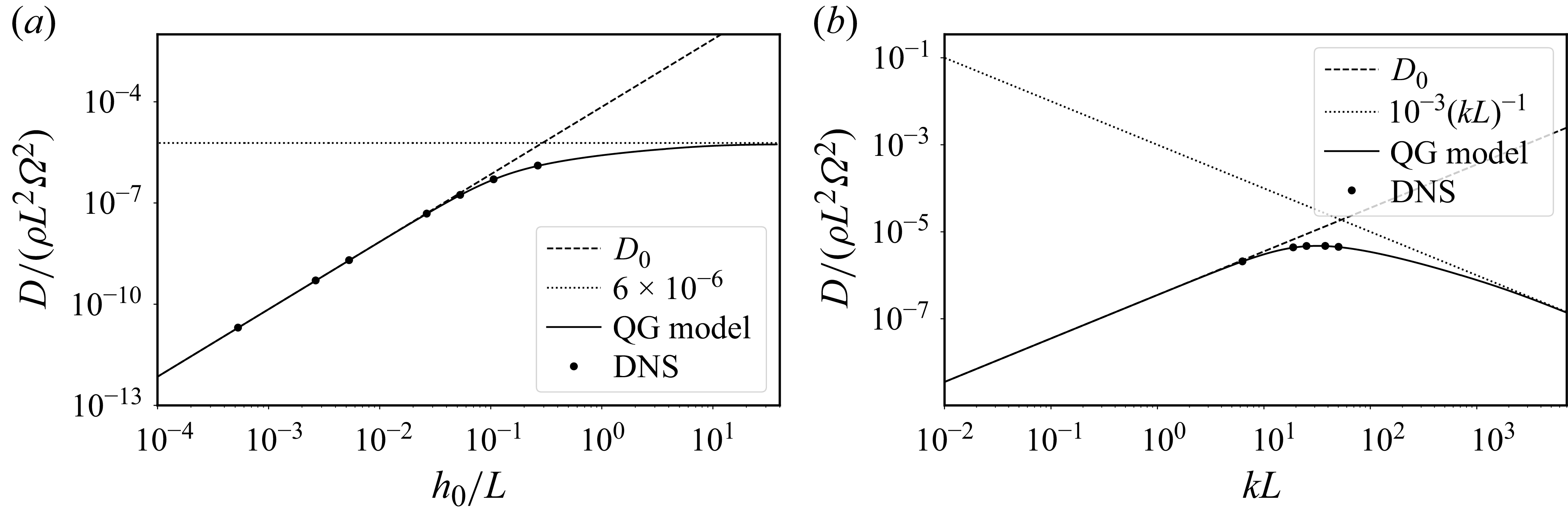
We now examine the drag for a steep topography in the geostrophic limit. In this regime, we expect the slope to play an important role. In practice, the slope can be varied at constant intrinsic frequency in two ways, by changing either the height or the wavelength of the topography. We present in figure 5 the drag predicted from the theoretical model and the drag computed from the simulations, as a function of the height
 $h_0$
at the fixed value
 $kL =6\pi$
, and as a function of
 $k$
at the fixed value
 $h_0/L =0.1$
. We observe a close agreement between the numerical simulations and the asymptotic theory over a broad range of non-trivial values of
 $h_0$
and
 $k$
, making us confident that the model can be used to explore a numerically inaccessible range of parameters. For small values of
 $h_0$
and
 $k$
, we recover the shallow drag
 $D_0$
as expected from the theory. As we increase the height of the topography at fixed
 $k$
(figure 5
a), the drag departs from the shallow value in agreement with the theoretical QG model, which predicts a saturation at large values of
 $h_0$
(not accessible numerically). In contrast, when increasing
 $k$
at fixed
 $h_0$
, the drag reaches a maximum for a critical wavenumber that is well captured by the DNS (figure 5
b), before decaying asymptotically as
 $D \propto k^{-1}$
at larger values of
 $k$
.
(a) Drag as a function of
 $h_0$
for
 $kL = 6\pi$
,
 $U_0/(\varOmega L) = 1.06 \times 10^{-5}$
and
 $E_{L} = 10^{-4}$
for the DNS. (b) Drag as a function of
 $k$
for
 $h_0/L = 0.1$
and
 $E_{L} = 10^{-4}$
in the DNS. Solid lines show steep QG model (3.21), dashed lines show shallow drag given by formula (3.14a
) and dotted lines indicate the asymptotic behaviour at large slopes.

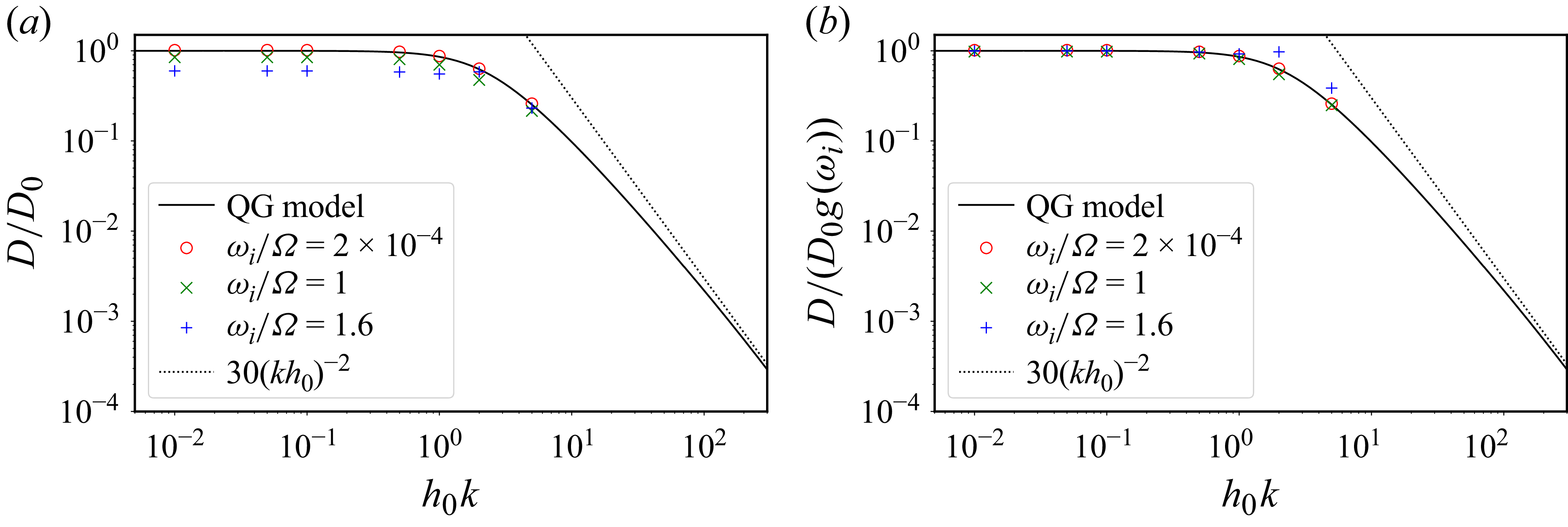
To understand these results, we examine the geometrical correction
 $f(h_0k)$
in (3.21), as shown in figure 6(a) for the fixed values
 $kL=6\pi$
and
 $\omega _i/\varOmega =2\times 10^{-4}$
and with
 $10^{-2} \lesssim h_0 k \lesssim 15$
. For shallow slopes, the drag follows the shallow approximation
 $f(h_0k)\sim 1$
. The steep nature of the topography manifests itself for
 $h_0k \gtrsim 0.5$
, and becomes nearly asymptotic at
 $h_0k\gtrsim 100$
, where the geometrical correction follows the scaling given by
 $D/D_0\sim (h_0k )^{-2}$
. Given the expression of
 $D_0\propto h_0(h_0k)$
, the geometrical correction is nearly constant
 $f(h_0k)\sim 1$
at low values of
 $h_0 k$
, and
 $D\propto h_0^2k$
. For larger slopes,
 $f(h_0k)\propto (h_0k)^{-2}$
and therefore
 $D\propto k^{-1}$
, explaining the aforementioned saturation and maximum drag at a critical wavenumber. Figure 6(b) shows the same function
 $f$
, but now compares it with the dimensionless drag simulations made by
 $D_0 g (\omega _i)$
. We observe that the analytical expression
 $D_0 f(h_0k) g(\omega _i)$
seems valid well beyond the asymptotic limit where it has been obtained. Indeed, it describes reasonably well the numerical results in the non-QG regime with an intrinsic frequency of
 $1$
. However, it fails at a higher intrinsic frequency of
 $1.6$
. This shows that the drag expression
 $D_0 f(h_0k) g(\omega _i)$
could be meaningful for certain weakly non-QG steep topographies.
Normalised pressure drags (a)
 $D/D_0$
and (b)
 $D/(D_0g(\omega _i))$
as a function of topography slope
 $h_0k$
, in the QG model and in DNS. The latter are performed at
 $kL = 6\pi$
,
 $\omega _i/\varOmega = 2\times 10^{-4}$
and
 $E_{L} = 10^{-4}$
.

Figure 6. Long description
Two line graphs depict normalized pressure drags as a function of topography slope. Panel A: The y-axis represents D/D0 and the x-axis represents h0k. The graph includes data for different values of ωi/Ω, specifically 2 times 10 to the power of -4, 1, and 1.6, along with a QG model and a dotted line representing 30(kh0)^2. Panel B: The y-axis represents D/(D0g(ωi)) and the x-axis represents h0k. Similar to Panel A, it includes data for different values of ωi/Ω and a QG model, along with a dotted line representing 30(kh0)^2. Both panels show how the normalized pressure drags vary with topography slope in different scenarios.
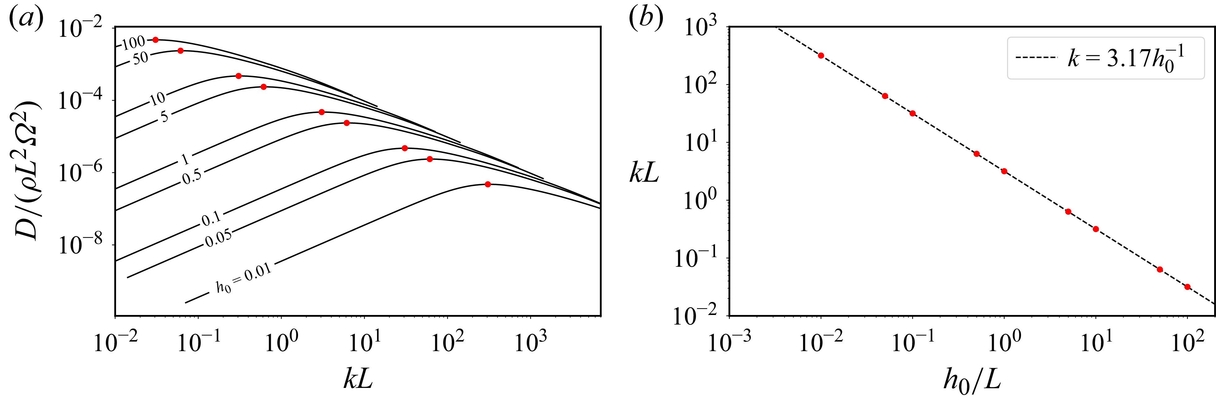
The critical topography wavenumber, at which we observe a maximum of the drag, is given by the maximum of
 $h_0 k f(h_0k)$
. We present in figure 7(a) the QG wave-driven drag as a function of
 $k$
for different values of the height
 $h_0$
. For each value of
 $h_0$
, we identify the critical wavenumber that corresponds to the maximum of the pressure drag. This critical value can then be represented as a function of
 $h_0$
(figure 7
b) suggesting that it follows a scaling of the form
 $k \propto h_0^{-1}$
. Using a linear regression we obtain the prefactor, and we predict that the maximum wave drag is obtained for topographies satisfying
 $h_0 k \sim 3.17$
.
(a) Drag as a function of
 $k$
for different values of
 $h_0/L$
and
 $U_0/(\varOmega L) = 10^{-4}$
. Positions of the maxima are represented by red markers. (b) Maximum drag in the
 $(h_0,k)$
plane, and fitted scaling law
 $k = 3.17 h_0^{-1}$
. Red markers are the same as in (a).

4.3. Velocity and pressure fields, and the transition from shallow to steep dynamics
The transition from the shallow to the steep regime is also accompanied by marked changes in the horizontal velocity and pressure. We present in figure 8 the horizontal cross-sections of the pressure and horizontal velocities (top row) and of the kinetic energy (bottom row), taken just above the topography for three representative wavenumbers
 $k L = [0.1, 31.7, 500]$
in the shallow case, the maximum-drag regime and the asymptotic steep limits, respectively. In addition, we mark with solid and dashed contour lines the projections of the topographic troughs and crests at
 $h = \pm 0.2h_0$
. In the shallow case, the pressure is dominated by a single wavenumber at
 $k$
(respectively at
 $2k$
for the kinetic energy), with the largest amplitude located near the regions of maximum slope. The horizontal flow remains smooth, forming clockwise vortices over positive pressure anomalies and counterclockwise vortices over negative ones. At
 $kL = 31.7$
, corresponding to the maximum drag for
 $h_0/L = 0.1$
, the pressure and velocity fields adopt a triangular pattern. The pressure distribution now diagonally separates the positive and negative topographic features, and the kinetic energy concentrates near the saddle point of the topography, indicating that the flow preferentially detours around the obstacle rather than passing over it. At the largest wavenumber
 $kL = 500$
, the flow and kinetic energy become confined along the line
 $y = 0.5\lambda = \pi /k$
, following a path of constant height, hence not producing any significant drag. The triangular pressure pattern sharpens into a stripe pattern with wavenumber
 $2k\,\boldsymbol{1}_{y}$
. In this asymptotic configuration, the pressure perturbations around the topographic bumps become symmetric and produce equal and opposite contributions to the drag, leading to a vanishing net force in both horizontal directions.
Pressure (top) and kinetic energy (bottom) from the QG model for (a–c) different wavenumbers
 $k$
at
 $h_0/L = 0.1$
, and
 $U_0/(\varOmega L) = 10^{-4}$
. Horizontal velocity is represented in a quiver on top of pressure. Positive bumps are represented using solid lines and negative bumps using dashed lines.

Figure 8. Long description
Panel A: The top graph is a heatmap showing pressure distribution with horizontal velocity represented as a quiver plot. The x-axis is labeled x/λ and ranges from 0 to 1. The y-axis is labeled y/λ and ranges from 0 to 1. The color scale ranges from -1 to 1, with red indicating positive values and blue indicating negative values. The bottom graph is a heatmap showing kinetic energy distribution. The x-axis is labeled x/λ and ranges from 0 to 1. The y-axis is labeled y/λ and ranges from 0 to 1. The color scale ranges from 1 x 10^-13 to 4. Positive bumps are represented using solid lines and negative bumps using dashed lines. Panel B: The top graph is a heatmap showing pressure distribution with horizontal velocity represented as a quiver plot. The x-axis is labeled x/λ and ranges from 0 to 1. The y-axis is labeled y/λ and ranges from 0 to 1. The color scale ranges from -5 to 5, with red indicating positive values and blue indicating negative values. The bottom graph is a heatmap showing kinetic energy distribution. The x-axis is labeled x/λ and ranges from 0 to 1. The y-axis is labeled y/λ and ranges from 0 to 1. The color scale ranges from 1 x 10^-8 to 7.5. Positive bumps are represented using solid lines and negative bumps using dashed lines. Panel C: The top graph is a heatmap showing pressure distribution with horizontal velocity represented as a quiver plot. The x-axis is labeled x/λ and ranges from 0 to 1. The y-axis is labeled y/λ and ranges from 0 to 1. The color scale ranges from -5 to 5, with red indicating positive values and blue indicating negative values. The bottom graph is a heatmap showing kinetic energy distribution. The x-axis is labeled x/λ and ranges from 0 to 1. The y-axis is labeled y/λ and ranges from 0 to 1. The color scale ranges from 1 x 10^-5 to 2. Positive bumps are represented using solid lines and negative bumps using dashed lines.
5. Discussion
5.1. Revisiting previous experimental results
The steep QG model presented in this study predicts that the wave pressure drag resulting from the flow past a topography reaches a maximum value when
 $k h_0 \simeq 3.17$
before decaying to zero as
 $k^{-1}$
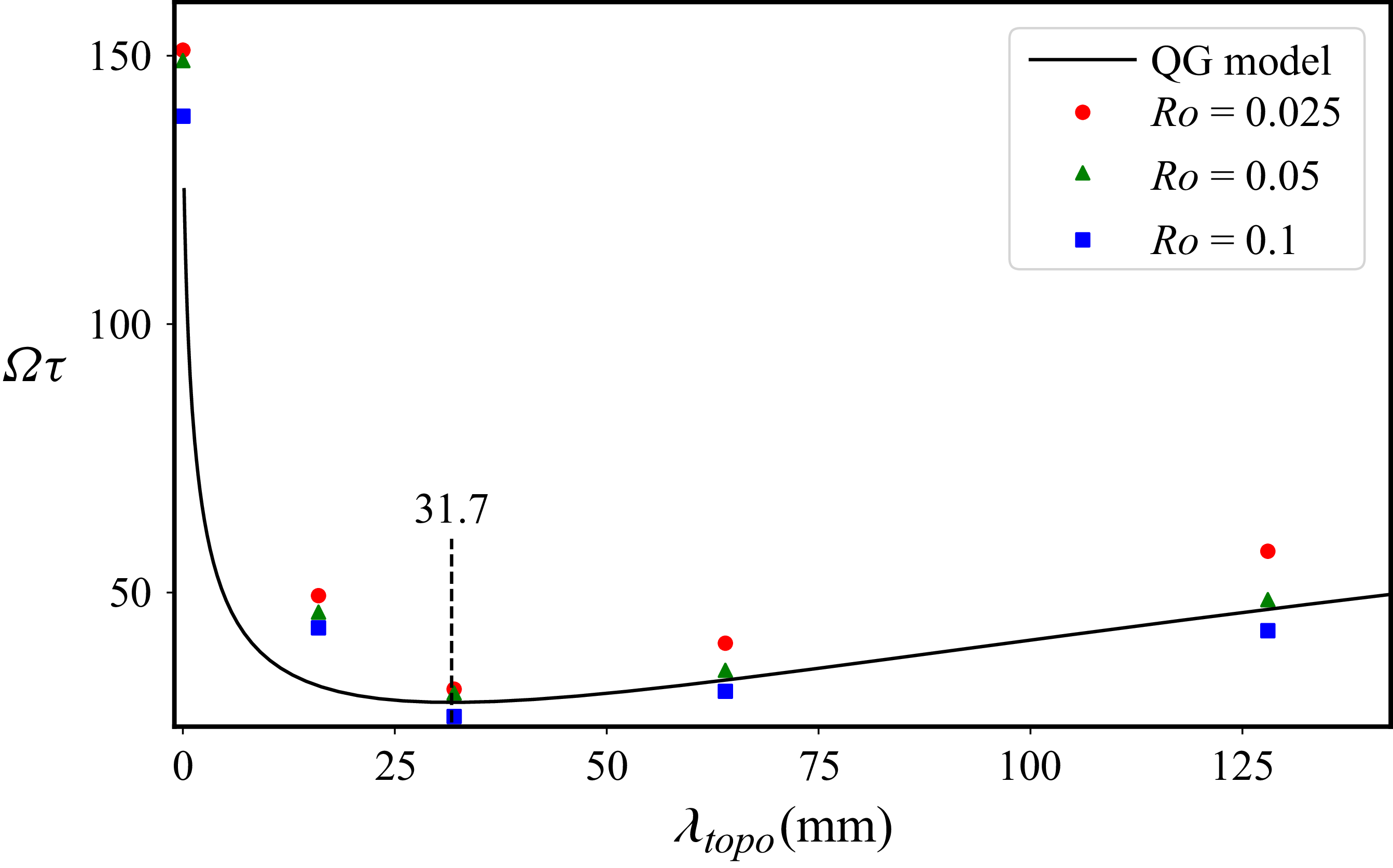
. This result sheds light on the previously published experimental results of Burmann & Noir (Reference Burmann and Noir2018), in which the authors conducted experiments to investigate the influence of topography on a rapidly rotating fluid. Specifically, they examined the spin-up process in a straight cylinder with a bottom topography built from square blocks, instead of a sinusoidal bump as in this study. To avoid any possible confusion, we thereafter refer to their topography as chessboard-like topography. They employed the spin-up time as an indirect measure of the torque. In their experiments, the height of the topography was held constant at
 $h_{\textit{topo}} = 16$
mm, while the horizontal wavenumber
 $\lambda _{\textit{topo}}$
of the topography was varied. They identified a minimum spin-up time at a critical wavelength of the topography, corresponding to a maximum torque and thus a maximum drag. Despite the topography having an infinite slope in the experiments, we propose, using an asymptotic steep QG model, to gain physical insight into their results.
To do so, we approximate the experimental square topography with an egg-box shape with a single-wavelength sinusoidal topography, characterised by
 $h_0 = h_{\textit{topo}} = 16$
mm and a wavenumber
 $k = 2\pi / \lambda _{\textit{topo}}$
. Unlike a uniform flow over a topography, the intrinsic frequency in this setting depends on the cylindrical distance
 $s$
(measured from the rotation axis) as
 \begin{equation} \frac {\omega _i}{\varOmega } = \frac {\delta \varOmega }{\varOmega } s k, \end{equation}
where
 $\delta \varOmega$
is the small increment of the rotation rate imposed during the spin-up of the fluid. The above intrinsic frequency reaches a maximum at the edge that never exceeds
 $\omega _i / \varOmega = 0.1$
, where the steep QG model remains applicable. The comparison between the asymptotic predictions and the experimental findings is shown in figure 9. The QG steep model predicts a maximum drag (and thus a maximum torque) for
 $h_0 k \sim 3.17$
, which corresponds to a wavelength
 $\lambda _{\textit{topo}} = 31.7$
mm for the height
 $h_{\textit{topo}} = 16$
mm used in the experiment. The predicted maximum quantitatively aligns with the observed minimum spin-up time reported in Burmann & Noir (Reference Burmann and Noir2018) as shown in figure 9.
Spin-up time as a function of the wavelength
 $\lambda _{\textit{topo}}$
of the chessboard-like topography considered in Burmann & Noir (Reference Burmann and Noir2018). Data were measured at fixed height
 $z/H = 0.53$
and
 $4\nu /(\varOmega H^2) = 5.4 \times 10^{-5}$
. Solid line shows theoretical spin-up time given by (5.2b
) for a steep topography.

By employing the wave drag per unit of surface derived from the steep QG model with
 $U_0 = \delta \varOmega s$
and
 $h_0 = 16$
mm, the pressure torque per unit of surface can be estimated at each cylindrical radius. Integrating over the topography’s disk, and calculating the boundary-layer viscous torque from both top and bottom surfaces, we obtain a total torque
 $\varGamma$
given by (in dimensional units)
 \begin{equation} \varGamma = \tau ^{-1} I \delta \varOmega , \quad \varOmega \tau = \left [ \left (\frac {4\nu }{\varOmega H^2} \right )^{1/2}+ \frac {h_0^2k }{4\sqrt {2}H}f(h_0k) \right ]^{-1}, \end{equation}
where
 $I=\rho \pi H R^4/2$
is the axial moment of inertia of the cylinder,
 $R$
is the outer cylindrical radius and
 $H$
is the cylindrical height. To obtain the spin-up time, we apply conservation of angular momentum to the fluid in a solid-body rotation at
 $\delta \varOmega$
such that
 \begin{equation} I \mathrm{d}_t (\delta \varOmega ) = -\varGamma . \end{equation}
The latter equation admits an exponentially decaying solution for
 $\delta \varOmega$
, with a characteristic time scale
 $\tau$
given from (5.2b
). We compare this spin-up time with the experimental observations of Burmann & Noir (Reference Burmann and Noir2018) in figure 9, obtaining a very good agreement between the predictions and the experimental data. This confirms that the asymptotic steep QG model can effectively capture the main physics governing the inertial-wave coupling with a steep topography when
 $\omega _i/\varOmega \ll 1$
.
5.2. Implications in geophysically relevant applications
The asymptotic theory, which has been validated against numerical simulations, could also be used to get some insight into more extreme geophysical conditions that are unreachable with simulations. In most geophysical fluid systems surrounded by solid layers (e.g. in planetary liquid cores or subsurface oceans of icy moons), the global Ekman number based on the depth of the fluid layer is typically of the order
 $\sim 10^{-15} {-} 10^{-10}$
. A typical topography at a fluid–solid interface, such as the Earth’s CMB, can have a height of a few kilometres over hundred to thousands of kilometres of lateral extent (e.g. Vidal et al. Reference Vidal, Noir, Cébron, Burmann, Monville, Giraud and Charles2024). Therefore, we can estimate the relative importance of the viscous to pressure drag using the asymptotic shallow theory. The expression of the viscous drag
 $D_v$
for a shallow topography, which is given in Appendix B, yields
 \begin{equation} \frac {D}{D_{\nu }} \approx \frac {(h_0k)^2}{2E_{\lambda }^{1/2}}\sqrt {1-\frac {\omega _i^2}{4\varOmega ^2}}. \end{equation}
Hence, we expect the pressure drag to be one order of magnitude greater than the laminar viscous drag atop the Earth’s liquid core for the largest topographic scales. On the contrary, the viscous drag is expected to remain the dominant one at small topographic wavelengths. Yet, we emphasise that our study has several limitations that currently prevent the quantitative extrapolation of the topographic torque at geophysical conditions. For instance, topography-driven waves were not assumed to interact with the topography after being emitted in the model, which is verified in the numerical simulations performed at finite values of the Ekman number. Because viscous wave damping is rather weak in geophysical conditions, we could instead expect wave reflections (or wave–topography interactions) that are not accounted for in current physical models. This again points to possible numerical or experimental extensions of the present study, in order to obtain a more complete picture. Furthermore, magnetic effects and density stratification have been entirely neglected (despite the potential impact on low-frequency motions at low Rossby numbers). We refer the interested reader to the study of Monville et al. (Reference Monville, Cébron and Jault2025) for a first step in this direction, which presents an asymptotic theory in the shallow regime accounting for the presence of a magnetic field and density stratification. It has also been suggested that the Ekman layer atop the Earth’s core may be turbulent (e.g. Cébron et al. Reference Cébron, Laguerre, Noir and Schaeffer2019; Buffett Reference Buffett2021) due to the slow precession of the Earth’s rotation axis, which may result in an increased turbulent viscous drag (e.g. Csanady Reference Csanady1967; Sous et al. Reference Sous, Sommeria and Boyer2013). In such conditions, the interaction between a topography and the turbulent Ekman layer remains largely unknown so far (e.g. for roughness, see Vidal et al. (Reference Vidal, Noir, Cébron, Burmann, Monville, Giraud and Charles2024)) and further investigations are necessary.
Nonetheless, our study also sheds new light into the long-standing geophysical question of the strength of the topographic torque
 $\boldsymbol{\varGamma }_{\!p}$
at the Earth’s CMB. Some temporal fluctuations in the Earth’s rotation are sustained by exchanges of angular momentum between the liquid core and the mantle, but the physical mechanisms responsible for such exchanges are not fully understood yet (e.g. Roberts & Aurnou Reference Roberts and Aurnou2012). In particular, the topographic torque
 \begin{equation} \boldsymbol{\varGamma }_{\!p} = \int _S p \boldsymbol{r} \times \hat {\boldsymbol{n}} \, \mathrm{d} S \end{equation}
at the Earth’s CMB, where
 $p$
is the pressure exerted on the solid mantle by the fluid, remains poorly constrained so far. Previous numerical simulations of turbulent convection with topography reported a linear scaling law
 $|\boldsymbol{\varGamma }_{\!p}| \propto h_0$
(Kuang & Chao Reference Kuang and Chao2001; Oliver et al. Reference Oliver, Blackman, Tarduno and Calkins2025), whereas various theoretical studies argued for a quadratic law
 $|\boldsymbol{\varGamma }_{\!p}| \propto h_0^2$
(Kuang & Bloxham Reference Kuang and Bloxham1993; Glane & Buffett Reference Glane and Buffett2018; Jault Reference Jault2020; Gerick et al. Reference Gerick, Jault, Noir and Vidal2020; Monville et al. Reference Monville, Cébron and Jault2025). Hence, these two scaling laws yield very different estimates for the topographic torque for realistic parameters. Actually, as pointed out in Oliver et al. (Reference Oliver, Blackman, Tarduno and Calkins2025), the two scaling laws can be valid depending on the pressure scaling. Since we have
 $|\hat {\boldsymbol{n}} \, \mathrm{d} S| = \mathcal{O}(h_0)$
at the leading order, we deduce from the above definition that
 \begin{equation} |\boldsymbol{\varGamma }_{\!p}| \propto \begin{cases} h_0 & \text{if $|p| = \mathcal{O}(1)$}, \\[5pt] h_0^2 & \text{if $|p| = \mathcal{O}(h_0)$}.\\ \end{cases} \end{equation}
This heuristic argument explains why the two scaling laws can be obtained in numerical simulations. In turbulent convection, the leading-order pressure is independent of the topography height, yielding the linear scaling. Conversely, the pressure has a topography-driven amplitude
 $\propto h_0$
in our set-up, resulting in the quadratic scaling.
6. Concluding remarks
We investigated in this work the inertial-wave drag resulting from a spatially uniform and steady flow over a sinusoidal topography. Using numerical simulations, we showed that the asymptotic analytical solution in the limit of a shallow topography with
 $h_0k \ll 1$
is valid in the whole range of inertial-wave frequency
 $0 \leqslant U_0 k/\varOmega \lt 2$
for sufficiently low values of the Ekman number. In this shallow limit, the drag reaches a maximum for
 $\omega _i/\varOmega =\sqrt {2}$
before rapidly decaying to zero as we approach
 $\omega _i/\varOmega =2$
. At the finite Ekman numbers achievable in the simulations, a viscous boundary-layer pressure drag becomes significant as we approach this limit. However, our results suggest that it should not be significant at the asymptotically low values of planetary cores and subsurface oceans. Further investigations at lower Ekman numbers might be necessary to confirm this behaviour unambiguously.
For finite-slope topography, we proposed a novel semi-analytical model for the wave-driven drag in the QG limit. This latter model has been validated by numerical simulations. Moreover, it was found to reproduce the indirect torque estimate from previous experimental results (Burmann & Noir Reference Burmann and Noir2018). We found that the steep nature of the topography occurs for slopes with
 $h_0 k \gtrsim 0.5$
, and an asymptotic behaviour independent of the height of the topography
 $h_0$
occurs at very large slopes. Our model predicts a maximum wave-driven drag for a critical slope with
 $h_0 k = 3.17$
, in good agreement with the numerical simulations and previous experimental observations. The latter value of
 $3.17$
has to be taken as a precise, semi-analytical measurement independent of the Ekman number (which should not be confused with
 $\pi$
, whose proximity is merely coincidental). Although this study focused on periodic monochromatic topographies, the methodology could be extended to more complex topographies. The critical slope and the minimal matrix size would then be different. For example, an egg-box topography with
 $k_{\!y} = 2k_x$
would mean that half of the
 $h_0k$
in the matrix would be replaced by
 $2h_0k$
. We believe our study can serve as a starting point to build upon towards more complex and more realistic conditions, including multiple wave reflections and density stratification (e.g. Abdulah & Kang Reference Abdulah and Kang2026; Abdulah et al. Reference Abdulah, Kang and Rekier2026).
Acknowledgements
The authors acknowledge the three anonymous reviewers for their positive and constructive reports, which helped in improving the quality of the manuscript.
Funding
V.G. is supported by ETH grant no. ETH-04 22-1. J.N. acknowledges Simons Foundation grant no. SFI-MPS-T-MPS-00007353. D.C. received funding from the ERC under the European Union’s Horizon 2020 research and innovation programme (THEIA project, grant agreement no. 847433). J.V. was partly supported by the Programme National de Planétologie (PNP) of CNRS-INSU, which is co-funded by CNES. All the numerical simulations have been carried out on the HPC cluster Euler from ETH.
Declaration of interests
The authors report no conflict of interest.
Data availability statement
The Nek5000 code is freely available at https://nek5000.mcs.anl.gov/.
Author contributions
V.G. ran the numerical simulations, conducted the asymptotic calculations and the data analysis and contributed to the writing of the paper. J.N. designed and supervised the project, sourced the funding for V.G. and contributed to the development of the analytical model, to the data analysis and to the writing of the paper. D.C. contributed to the analytical developments, to the data analysis and to the writing of the paper. J.V. designed the numerical model and contributed to the data analysis and to the writing of the paper. R.M. contributed to the shallow analytical theory and to the data analysis. All authors gave final approval for submission and agreed to be held accountable for the work performed therein.
Appendix A. Analytical details
A.1. Dispersion relation in the shallow model
The egg-box-like topography, which is a product of two sine functions as
 \begin{equation} h(x,y) = h_0\sin {(k x)}\sin {(k y)}, \end{equation}
can be rewritten as a sum of complex exponentials in the form
 \begin{equation} h(x,y) = \frac {h_0}{4} \left [ \mathrm{e}^{\mathrm{i}(k x-k y)}+ \mathrm{e}^{\mathrm{i}(-k x+k y)} - \mathrm{e}^{\mathrm{i}(k x+k y)} - \mathrm{e}^{\mathrm{i}(-k x-k y)} \right ]\!. \end{equation}
We consider only the case of a shallow topography, where
 $h_0k \ll 1$
. This allows us to approximate the topography to be at constant height
 $z = 0$
instead of
 $z = h$
. We also consider the linearised Navier–Stokes equations with
 $u \ll U_0$
. With these two considerations, boundary condition (3.15) simplifies to
 \begin{equation} u_z(x,y,0) = U_0 \partial _x h \quad \mbox{at}\quad z = 0. \end{equation}
By combining (A2) and (A3), the vertical velocity is given from the boundary condition by
 \begin{equation} u_z(x,y,0) = \frac {\mathrm{i} h_0 k U_0}{4} \left [ \mathrm{e}^{\mathrm{i}(k x-k y)}- \mathrm{e}^{\mathrm{i}(-k x+k y)} - \mathrm{e}^{\mathrm{i}(k x+k y)} + \mathrm{e}^{\mathrm{i}(-k x-k y)} \right ]\!. \end{equation}
Using the indices
 $m$
and
 $n$
, which can have the value
 $-1$
or
 $1$
, we can rewrite the boundary condition as an indexed sum given by
 \begin{equation} u_z(x,y,0) = \frac {- \mathrm{i} h_0 k U_0}{4} \sum _{m,n\in \{-1,1\}} n\mathrm{e}^{\mathrm{i}(mk x+nk y)}. \end{equation}
This boundary condition tells us that the forcing is stationary and can be expressed as a sum of four complex exponential functions. Consequently, we seek the unknown perturbations using a standing-wave ansatz as
 \begin{equation} \left [ \boldsymbol{u}, p \right ] (x,y,z) = \sum _{m,n\in \{-1,1\}} \left [\boldsymbol{u}_{m,n}, p_{m,n} \right ] \mathrm{e}^{\mathrm{i}( m k x + n k y + k_{z,m,n} z)} \end{equation}
with
 $\boldsymbol{u}_{m,n} = (u_{x,m,n}, u_{y,m,n}, u_{z,m,n})^\top$
. An expression for
 $u_{z,m,n}$
is then given by the boundary condition as
 \begin{equation} u_{z,m,n} = -\frac {n\mathrm{i} h_0 k U_0}{4} . \end{equation}
This is a linear problem, such that the solution of the sum of these four exponentials is the sum of the solutions for each exponential. Linearised equations (3.1a
,
b
) for each of orders
 $m,n$
can be rewritten as four linear equations for the coefficients
 $[u_{x,m,n}, u_{y,m,n}, u_{z,m,n}, p_{m,n}]$
as
 \begin{align} \big [ \mathrm{i} m k U_{0} + \nu K^2 \big ] u_{x,m,n} - 2 \varOmega u_{y,m,n} + \mathrm{i}m k p_{m,n} &=0, \\[-12pt]\nonumber \end{align}
 \begin{align} 2 \varOmega u_{x,m,n} + \big [ \mathrm{i} m k U_{0} + \nu K^2 \big ] u_{y,m,n} + \mathrm{i}n k p_{m,n} &= 0, \\[-12pt]\nonumber \end{align}
 \begin{align} \big [ \mathrm{i} m k U_{0} + \nu K^2 \big ] u_{z,m,n} + \mathrm{i} k_{z,m,n} p_{m,n} &= 0, \\[-12pt]\nonumber \end{align}
 \begin{align} m k u_{x,m,n} + n k u_{y,m,n} + k_{z,m,n} u_{z,m,n} &= 0 \end{align}
with
 $K^2 = 2k^2+k_{z,m,n}^2$
. These equations can be written in condensed matrix form as
 \begin{equation} \begin{pmatrix} \mathrm{i}m\omega _i + \nu K^2 & -2 \varOmega & 0 & \mathrm{i}m k \\[9pt] 2\varOmega & \mathrm{i}m\omega _i + \nu K^2 & 0 & \mathrm{i}n k \\[9pt] 0 & 0 & \mathrm{i}m\omega _i + \nu K^2 & \mathrm{i} k_{z,m,n} \\[9pt] mk & nk & k_{z,m,n} & 0 \end{pmatrix} \begin{pmatrix} u_{x,m,n} \\[9pt] u_{y,m,n} \\[9pt] u_{z,m,n} \\[9pt] p_{m,n} \end{pmatrix} = 0, \end{equation}
where
 $\omega _i= U_{0} k$
is the intrinsic frequency. The dispersion relation of the waves is obtained by computing the determinant of the system (A9). It yields the dispersion relation of viscous inertial waves given by
 \begin{equation} K^2 \big [ m\omega _i -\mathrm{i}\nu K^2 \big ]^2 = 4 \varOmega ^2 k_{z,m,n}^2, \end{equation}
which reduces to (3.6) when
 $E_\lambda$
is introduced. In the limit of vanishing viscous effects, we recover the classical dispersion relation of inertial waves given by
 \begin{equation} \left (\frac {m \omega _i}{2\varOmega } \right )^2 = \frac {k_{z,m,n}^2}{K^2}, \end{equation}
in agreement with (1.1).
The viscous dispersion relation is a bicubic polynomial equation that has three solutions denoted by
 $\pm [k_{z,1}^2,k_{z,2}^2,k_{z,3}^2]$
, where
 $k_{z,1}^2$
is the ‘bulk mode’ and
 $[k_{z,2}^2,k_{z,3}^2]$
are rapidly decaying modes in the interior. As expected, the bulk solution reduces to the inviscid one when
 $E_\lambda \rightarrow 0$
(not shown). In addition, the wavenumber follows an asymptotic scaling behaviour when
 $\omega _i /\varOmega \gg 2$
, whose leading-order term is given by
 \begin{equation} \frac {k_{z,1}}{k} \approx \pm \sqrt {- \mathrm{i} \frac {m}{E_\lambda } \frac {\omega _i}{\varOmega }}. \end{equation}
This change in the behaviour of
 $k_z$
is likely associated with a change in the value of the drag, which might support the results indicated in figure 4.
A.2. Solving for the pressure coefficients in the steep QG model
We rewrite recurrence relation (3.18) in matrix form as
 \begin{equation} \begin{bmatrix} \sqrt {2} & 0 & 0 & 0 & \dfrac {h_0k}{2} & \dfrac {-h_0k}{2} & 0 & 0 & {\cdots} \\[9pt] 0 & \sqrt {2} & 0 & 0 & 0 & \dfrac {-h_0k}{2} & \dfrac {h_0k}{2} & 0 & {\cdots} \\[9pt] 0 & 0 & \sqrt {2} & 0 & \dfrac {h_0k}{2} & 0 & 0 & \dfrac {-h_0k}{2} & {\cdots} \\[9pt] 0 & 0 & 0 & \sqrt {2} & 0 & 0 & \dfrac {h_0k}{2} & \dfrac {-h_0k}{2} & {\cdots} \\[9pt] \vdots & & & & \ddots & \\[9pt] \vdots & & & & \ddots & \ddots \\[9pt] \vdots & & & & \ddots & & \ddots \\[9pt] \vdots & & & & \ddots & & &\ddots \\[9pt] \vdots & & & & \ddots & & & & \sqrt {m^2+n^2}\\[9pt] \vdots & & & & \ddots & & & & & \ddots \\ \end{bmatrix} \underbrace {\begin{bmatrix} p_{1,1} \\[9pt] p_{1,-1} \\[9pt] p_{-1,1} \\[9pt] p_{-1,-1} \\[9pt] p_{0,2} \\[9pt] p_{2,0} \\[9pt] p_{0,-2} \\[9pt] p_{-2,0} \\[9pt] \vdots \\[9pt] p_{m,n} \\[9pt] \vdots \\[9pt] p_{M,M} \end{bmatrix}}_{\boldsymbol{p}} = \mathrm{i}\sqrt {2}p_0 \underbrace {\begin{bmatrix} -1 \\[9pt] 1 \\[9pt] -1 \\[9pt] 1 \\[9pt] 0 \\[9pt] 0 \\[9pt] 0 \\[9pt] 0 \\[9pt] \vdots \\[9pt] 0 \\[9pt] \vdots \\[9pt] 0 \end{bmatrix}}_{\boldsymbol{c}}, \end{equation}
with
 $p_0 = \rho h_0 \varOmega \omega _i/(2\sqrt {2}k)=\rho h_0 \varOmega U_0/ (2\sqrt {2})$
. By multiplying both sides by
 $h_0k/\sqrt {2}$
, we rewrite the above linear system as
 \begin{equation} \unicode{x1D643}(h_0 k)\boldsymbol{\cdot }\boldsymbol{p} = \mathrm{i} D_0 \boldsymbol{c}, \end{equation}
where
 $ \unicode{x1D643}$
is a
 $M^2 \times M^2$
matrix depending on
 $h_0 k$
and
 $D_0$
is the shallow drag in the geostrophic limit given in (3.13b
). We then invert the matrix
 $ \unicode{x1D643}$
numerically to finally obtain the pressure coefficients as
 $\boldsymbol{p} = \mathrm{i} D_0 \unicode{x1D643}^{-1}\boldsymbol{\cdot }\boldsymbol{c}$
.
Appendix B. Boundary-layer effects
In addition to the inviscid inertial-wave drag, the boundary layer could also contribute to the drag at the small but yet finite Ekman number in the simulations. In this appendix, we use the results for the wavenumbers in the boundary layer derived by Machicoane et al. (Reference Machicoane, Labarre, Voisin, Moisy and Cortet2018) to estimate the viscous drag in the case of a shallow topography
 $h_0k \ll 1$
. We impose the no-slip boundary condition at
 $z=0$
, yielding
 \begin{equation} \boldsymbol{U} + \boldsymbol{u}_{\textit{i}w} + \boldsymbol{u}_{\textit{bl}} = \boldsymbol{0} \quad \mbox{at}\quad z = 0, \end{equation}
where
 $\boldsymbol{u}_{\textit{i}w}$
is the velocity field associated with inertial waves and
 $\boldsymbol{u}_{\textit{bl}}$
is the boundary-layer velocity to be determined. Assuming that
 $\boldsymbol{u}_{\textit{i}w}$
is given by the inviscid solution, the expression for
 $\boldsymbol{u}_{\textit{bl}}$
at the topography is given by
 \begin{equation} \boldsymbol{u}_{\textit{bl}}|_{z=0} = -U_0 \boldsymbol{1}_x - \boldsymbol{u}_{\textit{i}w}|_{z=0}. \end{equation}
Using the shallow approximation, we can simplify this expression to
 \begin{equation} \boldsymbol{u}_{\textit{bl}}|_{z=0} = -U_0 \boldsymbol{1}_x + \mathcal{O}(U_0h_0k). \end{equation}
Since
 $U_0 \boldsymbol{1}_x$
has a wavenumber
 $m=0$
, the corresponding
 $m\omega _i$
for the shallow boundary layer is also zero. With the boundary-layer vertical wavenumbers (Machicoane et al. Reference Machicoane, Labarre, Voisin, Moisy and Cortet2018)
 \begin{align} k_{z,\textit{bl},+} &= \frac {1+\mathrm{i}}{2} \sqrt {2-\frac {m\omega _i}{\varOmega }} \frac {k}{E_{\lambda }^{1/2}} + \mathcal{O}(E_{\lambda }), \end{align}
 \begin{align} k_{z,\textit{bl},-} &= \frac {-1+\mathrm{i}}{2} \sqrt {2+\frac {m\omega _i}{\varOmega }} \frac {k}{E_{\lambda }^{1/2}} + \mathcal{O}(E_{\lambda }), \end{align}
which can be simplified in the QG limit
 $\omega _i/\varOmega \ll 1$
into
 \begin{align} k_{z,\textit{bl}} \approx \frac {\pm 1+\mathrm{i}}{\sqrt {2}} \frac {k}{E_{\lambda }^{1/2}}, \end{align}
the boundary-layer flow is given at
 $\mathcal{O}(U_0h_0k)$
by
 $\boldsymbol{u}_{\textit{bl}} \approx u_{x,\textit{bl}} \boldsymbol{1}_x + u_{y,\textit{bl}} \boldsymbol{1}_{y}$
with
 \begin{equation} u_{x,\textit{bl}} \approx -U_0 \cos {\left (\frac {1}{\sqrt {2}} \frac {k}{E_{\lambda }^{1/2}} z\right )} \mathrm{e}^{ -\frac {1}{\sqrt {2}} \frac {k}{E_{\lambda }^{1/2}} z}, \quad u_{y,\textit{bl}} = U_0 \sin {\left (\frac {1}{\sqrt {2}} \frac {k}{E_{\lambda }^{1/2}} z \right )} \mathrm{e}^{ -\frac {1}{\sqrt {2}} \frac {k}{E_{\lambda }^{1/2}} z}. \end{equation}
Next, from the definition of the viscous force
 $\boldsymbol{F}_\nu$
per unit of surface acting on the topography (e.g. Roberts & Aurnou Reference Roberts and Aurnou2012), we can estimate the viscous drag
 $D_\nu \geqslant 0$
per unit of surface in the
 $x$
direction as
 $\boldsymbol{F}_\nu \boldsymbol{\cdot } \boldsymbol{1}_x = -D_\nu \boldsymbol{1}_x$
. It yields at the leading order
 \begin{equation} D_v \approx \rho \nu \left . \partial _z u_{x,\textit{bl}} \right |_{z=0} = \rho \nu \frac {U_0}{\sqrt {2}} \frac {k}{E_{\lambda }^{1/2}} = \rho \frac {\omega _i \varOmega E_{\lambda }^{1/2}}{\sqrt {2}k^2}. \end{equation}
Finally, we can recast the viscous drag on a shallow topography as
 \begin{equation} \frac {D_v}{D_0} \approx \frac {2 E_{\lambda }^{1/2}}{(h_0k)^2}. \end{equation}
At the first order, the viscous boundary layer does not generate a pressure field, because it results from the balance between the Coriolis acceleration and viscous forces. A pressure field only emerges as a second-order perturbation, when looking at the viscous boundary-layer correction for inertial waves. According to the Navier–Stokes equations projected onto the
 $z$
axis, the second-order pressure would scale as
 $\rho \nu k_{z,\textit{bl}} u_{\textit{i}w}$
and would be proportional to
 $\rho \sqrt {E_{\lambda }} \varOmega h_0 U_0(2\pm \omega _i/\varOmega )^{-1/2}$
. The resulting pressure drag in the
 $x$
direction would scale as
 $ \sqrt {E_{\lambda }} D_0$
, which is always smaller by a factor
 $\sqrt {E_{\lambda }}$
compared with the inertial-wave pressure drag. Therefore, we neglect this contribution in the main text. This ratio is not valid near the evanescent limit where
 $\omega _i \approx 2\varOmega$
, and the factor
 $(2\pm \omega _i/\varOmega )^{-1/2}$
is no longer of unit order. Around this value, we have not determined the sign in the expression and it may be possible that the secondary drag corresponds to the strange behaviour seen in figure 4.

 U0=U01x
 h(x,y)=h0sin(kx)sin(ky)
 k
 λ=2π/k
 L2

 (ωi/Ω,h0k)
 y=π/(2k)

 y=π/(2k)
 D/D0
 ωi/Ω
 EL=ν/(ΩL2)=Eλ/(Lk)2
 h0
 kL=6π
 U0/(ΩL)=1.06×10−5
 EL=10−4
 k
 h0/L=0.1
 EL=10−4
 D/D0
 D/(D0g(ωi))
 h0k
 kL=6π
 ωi/Ω=2×10−4
 EL=10−4
 k
 h0/L
 U0/(ΩL)=10−4
 (h0,k)
 k=3.17h0−1

 k
 h0/L=0.1
 U0/(ΩL)=10−4
 λtopo
 z/H=0.53
 4ν/(ΩH2)=5.4×10−5

 Open access

