1. Introduction
Multi-machine coordination is the inevitable step for thin-walled sheet metal part stamping in the automobile, aerospace, marine, and other fields [Reference Yu, Wang, Zhang, Zhang and Zhang1]. As the intelligent feeding device, it directly determines the work efficiency of the stamping line by constraint detection, trajectory planning, and performance optimization.
Avoiding collisions is the basic condition for the continuous operation of multiple coordinated machines. Collision detection [Reference Yousefizadeh and Bak2, Reference Haddadin, De Luca and Albu-Schäffer3] includes three aspects: collision prediction, collision supervision, and collision feedback. Collision feedback is the combination of collision prediction and collision supervision. In the collision prediction, distance calculation can sufficiently identify the shortest distance between the target machine and obstacle to reduce the risk of collision [Reference Tang, Zhou, Zhang, Liu, Liu and Ding4–Reference Römer, Fidlin and Seemann7]. Common methods of distance calculation are based on Euclidean distance, cosine similarity, Manhattan distance, Haversine, and other mathematical models. In the collision supervision [Reference Haddadin, De Luca and Albu-Schäffer3], various sensors such as displacement sensor, force sensor, and torque sensor are utilized to detect the possibility of collision occurrence [Reference Ebrahimi, Norouzi, Dastres, Faieghi, Naderi and Malekzadeh8, Reference Feng, Tian, Li and Jiang9]. The work efficiency of collision supervision is greatly affected by the reliability, resolution, and sensitivity of sensors. Compared with mobile robots in Cartesian space [Reference Das, Sanyal and Mandal10], the collision detection of multi-link manipulators in joint space relies on the complex combination of distance calculation models and detection sensors.
For the multi-machine coordination in the dynamic compact environment, trajectory planning methods are divided into centralized trajectory planning methods [Reference Yamashita, Arai, Ota and Asama11, Reference Yang, Dong and Dai12] and distributed trajectory planning methods [Reference Gao, Li, Wang and Liu13–Reference Meng, Sun, Liu and Chi15]. Compared with centralized trajectory planning, distributed trajectory planning is easier to generate satisfactory solutions by trajectory optimization. Gravell and Summers demonstrated a feasible centralized technique for generating collision-free trajectories of multiple robots. Numerical experiments confirmed that the method significantly reduced the total time required for task execution [Reference Yang, Dong and Dai12]. Combined with the gradient projection algorithm and Hungarian algorithm, the distributed optimization method proposed by Huang was used to minimize the formation distance. Simulation and experimental results showed that the generated path was effective [Reference Huang, Zhou, Tu, Yao and Liu14].
Common indicators of performance optimization include collision avoidance [Reference Maghami, Imbert, Côté, Monsarrat, Birglen and Khoshdarregi16, Reference Deng, Ni, Zhang and Wang17], singularity avoidance [Reference Pham, Hamelin, Hazel and Z.Liu18], vibration suppression [Reference Wu, Tang, Xin, Wang, Peng and Yan19, Reference Boscariol, Richiedei and Tamellin20], and time-energy-jerk optimization [Reference Benotsmane, Dudás and Kovács21]. Collision avoidance algorithm include artificial potential field [Reference Ding, Zheng, Liu, Guo and Guo22], circular field [Reference Becker, Lilge, Müller and Haddadin23], and reinforcement learning [Reference Gómez, González, Martínez-Marín, Meziat and Sánchez24]. Much attention has been paid to performance optimization based on time-optimal trajectories [Reference Fan, Jia, Zhang, Zhou, Du, Liu, Cao and Zhang25, Reference Chettibi26] and smooth trajectories [Reference Wang, Hu, Zhou, He and Zhu27]. Yu et al. proposed a variable-time smooth interpolation method to locally optimize the fluctuation period and simultaneously generate high-performance trajectories in Cartesian and joint space [Reference Yu, Zhou and Huang28]. For the five degree-of-freedom robot arm, Rabab et al. proposed a new whip-lashing method to realize an optimal trajectory with minimal cycle time and smooth motion [Reference Benotsmane, Dudás and Kovács21]. Shao et al. proposed a novel two-stage goal selection algorithm, including the exploitation of the trajectory optimization and the goal set, to generate smooth trajectory during optimization [Reference Shao, Liao, Zhu, Zhang and Song29]. To improve the work efficiency, reduce energy consumption, and suppress vibration, Chen presented the multi-node time-energy-jerk trajectory optimization technology for high-speed parallel manipulators [Reference Chen, Wang, Liu and Jiang30]. Simulation and experimental results confirmed the effectiveness of the proposed method for trajectory performance optimization in refs. [Reference Yu, Zhou and Huang28–Reference Chen, Wang, Liu and Jiang30].
The above research shows that multi-robot trajectory planning has been widely studied and significant progress has been made in multi-objective trajectory optimization. However, compared with global trajectory optimization, efficient local trajectory optimization of the coordinated multi-link manipulator in the narrow feeding scenario is rarely focused on. Meanwhile, the work efficiency of the feeding manipulator is generally significantly higher than that of the multi-machine coordination in the whole stamping line. Under this circumstance, an analytical reinforcement method is proposed to optimize the trajectories in collision areas while keeping the rest of the trajectory unchanged. The unchanged parts of the trajectory serve as a local support, ensuring stability and continuity in the overall operation. Ultimately, the collision-free trajectory with local support performance is generated. Compared with the existing methods, main contributions of this paper include following aspects:
-
1. Rapid distance calculation equation based on collision-free gradient optimization function;
-
2. Multi-machine coordinated emergency smooth collision avoidance by local optimal strategy;
-
3. The consistent work efficiency between single manipulator and the whole stamping line.
The rest of the paper is organized as follows. Section 2 introduces some preliminary work such as problem formation and optimization, collision-free gradient optimization function, and local support strategy. Section 3 introduces detailed steps of the proposed method. Section 4 uses the case study to verify the effectiveness of the proposed method. Sections 5 and 6 are discussion and conclusions, respectively.
2. Preliminary work
2.1. Problem formation and optimization
Due to the limited working space, collision-free trajectories of multiple high-speed machines are difficult to coordinate in a dynamic narrow space. As shown in Figure 1, several feeding manipulators and stamping stations are alternately coordinated in the planar flexible stamping line. The sheet metal part to be stamped is transferred by the end-effector of the coordinated manipulator. It is transformed from the whole large part into discrete small parts.
Multi-machine coordination in the stamping line.

The work efficiency of multi-machine coordination is greatly affected by the width of sheet metal parts and upper dies. The original sheet metal part in Figure 1 is placed into the leftmost stamping station by the manipulator. As the stamping process advances from the leftmost stamping station to the rightmost stamping station, the width of the sheet metal part becomes smaller and smaller. The larger the width of sheet metal parts and upper dies, the longer the time occupied by the coordinated manipulator in the stamping station. Due to the insufficient handling space, dies and coordinated manipulators are prone to collision. In this case, the leftmost manipulator is more likely to collide with the upper die in the stamping station. The coordination between the leftmost manipulator and its adjacent upper die is the bottleneck factor to improve the work efficiency of the stamping line.
The contour is the key indicator to judge whether two machines collide. As shown in Figure 2, the contour of the upper die is generally arched in the depth direction. The coordinated manipulator handles the sheet metal part at the middle of the stamping station. Its working area is located in the horizontal direction of the vertical space in Figure 3(a). To further improve the work efficiency of the multi-machine coordination, irrelevant terminal bodies in the stamping station are ignored. The projection and its contour of extracted dies in the vertical space are shown in Figure 3(a). Affected by the working area of the coordinated manipulator in the depth direction, the projection of the extracted die is stretched. The initial models of upper die and lower die in Figure 2 are simplified to Figure 3(b).
The cross-section of the arch structure.

Model simplification.

The contour is the key indicator to judge whether two machines collide. As shown in Figure 2, the contour of the upper die is generally arched in the depth direction. The coordinated manipulator handles the sheet metal part at the middle of the stamping station. Its working area is located in the horizontal direction of the vertical space in Figure 3(a). To further improve the work efficiency of the multi-machine coordination, irrelevant terminal bodies in the stamping station are ignored. The projection and its contour of extracted dies in the vertical space are shown in Figure 3(a). Affected by the working area of the coordinated manipulator in the depth direction, the projection of the extracted die is stretched. The initial models of upper die and lower die in Figure 2 are simplified to Figure 3(b).
2.2. Collision-free gradient optimization function
Uncertain factors such as vibration, assembly error, and control failure may occur in the high-speed coordination manipulator. They exacerbate the possibility of collision between collision-free multiple machines in the simulation environment. And the work efficiency of multi-machine coordination is seriously affected. To this issue, safety distance based on Dijkstra algorithm [Reference Yao, Zhang, Shi, Li, Liang, Li and Huang31] is used to detect distance of multiple machines. The Dijkstra algorithm is a typical single-source shortest path algorithm, it determines the shortest path from one point to all the other points. However, it takes a long time to find the shortest distance between current dynamic machines by using traversal principle. To evaluate multi-machine distance efficiently, the collision-free gradient optimization function based on the circle envelope method is proposed. It uses the one-level operation in mathematics to judge the collision between the target contour and gradient contour. Considering the varying collision probabilities at different positions on the machine, corresponding distances are established on distinct positions. It results in a gradient contour, which is characterized by a gradual change in distance from the initial contour, with greater distances set in areas of higher collision probability and smaller distances in areas of lower collision probability. The gradient contour is generated from the dynamically constrained contour based on the circle envelope method. As shown in Eq. (1), machine can be represented as discrete contour points.
 \begin{equation} M_{T}=\left\{\left(x_{i},y_{i}\right)\left| 1\leq i\leq n,n\in Z\right.\right\} \end{equation}
where x i and y i are coordinates of the i-th contour point in the horizontal and vertical directions, respectively. n is the number of discrete contour points. Z represents an integer. M is short for machine. T is the machine type.
For example, M u represents contour points of the upper die in Figure 4(a). The gradient value g represents the radius of a circle, which is determined by experimental data. It is the key to evaluate the collision of multiple machines. x i and y i in Eq. (1) are taken as the circle center. As shown in Figure 4(b), the gradient circle C g with radius g is generated based on Eq. (2).
 \begin{equation} C_{g}=\left\{\begin{array}{ll} \left\{\left(x_{i},y_{i},g\right)\left| 1\leq i\leq n,n\in Z\right.\right\}, &\,{\rm if}\ y_{i}=y_{i}^{\min }\\ \left\{\left(x_{i},y_{i},0\right)\left| 1\leq i\leq n,n\in Z\right.\right\},&\,{\rm else} \end{array}\right. \end{equation}
where
 $y_i^{\rm min}$
is the minimum value of contour points with identical x
i
. It is obtained in Eq. (3).
Generation of the gradient contour.

 \begin{equation} y_{i}^{\min }=\min \left\{y_{j}\left| x_{i}=x_{j},1\leq j\leq n\right.\right\} \end{equation}
Contour crossing exists in adjacent gradient circles. As the target machine, the coordinated manipulator handles the sheet metal part between the upper die and the lower die. The upper die acts as the dynamic constrained machine to limit the handling space of the coordinated manipulator. In this case, combined with Eq. (4), adjacent gradient circles in Figure 4(b) are converted to the gradient contour in Figure 4(c).
 \begin{equation} \left(x_{i}^{C},\,y_{i}^{C}\right)=\left(x_{i}^{C_{g}},\,\min \left\{y_{j}^{C_{g}}\left|\,x_{i}^{C_{g}}=x_{j}^{C_{g}},\,1\leq j\leq n_{C}\right.\right\}\right) \end{equation}
where
 $x_i^C$
and
 $y_i^C$
are coordinates of the gradient contour in the horizontal and vertical directions, respectively.
 $x_i^{Cg}$
and
 $y_i^{Cg}$
are coordinates of points in crossing gradient circles in the horizontal and vertical directions, respectively. n
C
is the number of points in crossing gradient circles.
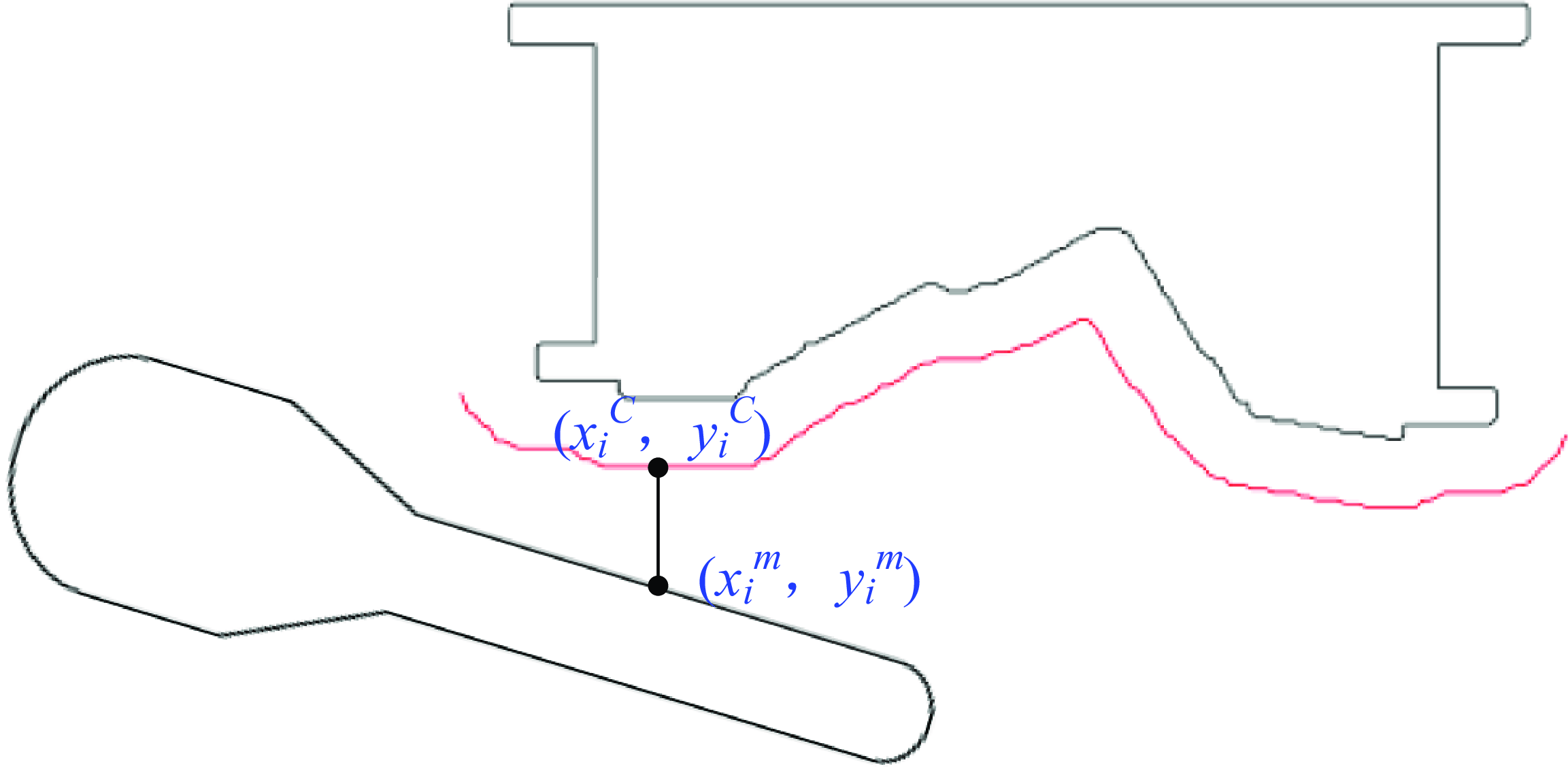
As shown in Eq. (5), the minimum distance d t between the target manipulator and the gradient contour is directly obtained by using the one-level operation in mathematics. If d t in Eq. (5) is greater than zero, the coordinated manipulator in Figure 5 will not collide with the upper die. Otherwise, the manipulator may collide with the upper die.
 \begin{equation} d_{t}=\min \left\{y_{i}^{C}-y_{i}^{m}\left|\, x_{i}^{C}=x_{i}^{m},1\leq i\leq n_{t}\right.\right\} \end{equation}
where
 $x_i^m$
and
 $y_i^m$
are coordinates of the target manipulator in the horizontal and vertical directions, respectively. n
t
is the number of points at time t where the target manipulator has the same horizontal coordinate as the gradient contour.
Distance detection in the stamping station.

2.3. Local support strategy
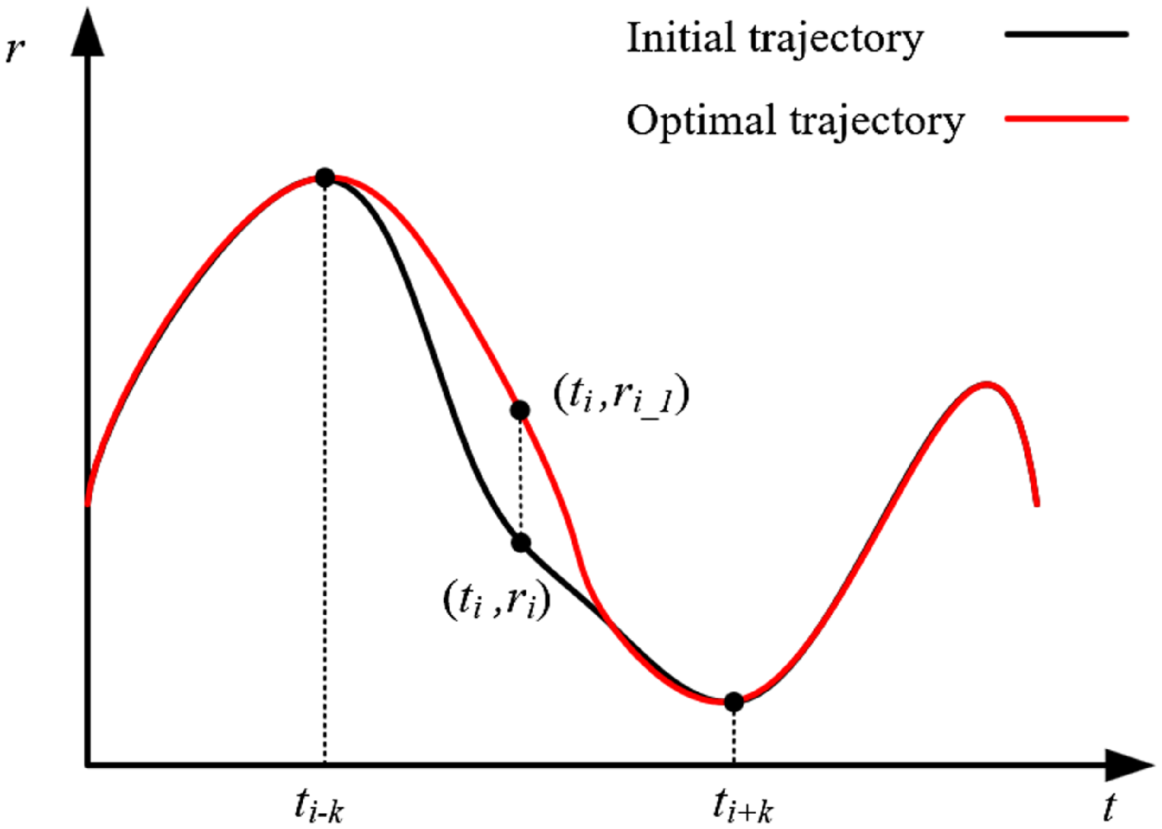
The coordinated manipulator handles the sheet metal part in the narrow dynamic space. The multi-machine collision is easy to occur. A time-displacement curve of certain joint is shown in Figure 6, where t is time and r is displacement. It is assumed that a multi-machine collision occurs at the time interval t i-k and t i+k . The black curve is the initial collision trajectory of the coordinated manipulator in joint space. To ensure the continuous periodic running of multiple machines, the collision trajectory is optimized to the collision-free trajectory represented by the red curve. Outside the time interval t i-k to t i+k , the performance of the initial and optimal trajectories is consistent. It includes displacement, velocity, acceleration, and other higher derivatives. In this case, control points (t i-k , r i-k ) and (t i+k , r i+k ) in Figure 6 divide the whole spatial-temporal region into local support region and local optimization region. The local optimization region is at the time interval t i-k and t i+k .
The initial and optimal displacement of the coordinated manipulator in joint space.

As shown in Eq. (6), there is a path point set P t in the local optimization region.
 \begin{equation} P_{t}=\left\{\left(t_{j},r_{j}\right)\left|\,i-k\leq j\leq i+k,i,j,k\in Z\right.\right\} \end{equation}
where t i and r i are time and displacement, respectively. i is the labeled point number in the middle of the local optimization region. k is the half number of elements in P t .
Due to abrupt changes of position and time at control points (t
i-k
, r
i-k
) and (t
i+k
, r
i+k
), the trajectory performance is significantly reduced. To ensure the smooth transition of trajectory performance between local support region and local optimization region, some auxiliary control points are added. P
t
in Eq. (6) is transformed into
 $P_{t}^{\prime}$
in Eq. (7). As shown in Figure 6, the path point set
 $P_{t}^{\prime}$
consists of the optimal trajectory in the local optimization region.
 \begin{equation} {P_{t}}^{\prime}=\left\{\begin{array}{l} \left\{\left(t_{i-k-l},r_{i-k}\right)\left| 1\leq l\leq L,l,L\in Z\right.\right\}\\ \left\{\left(t'_{j},r'_{j}\right)\left| i-k\leq j\leq i+k,i,j,k\in Z\right.\right\}\\ \left\{\left(t_{i+k+l},r_{i+k}\right)\left| 1\leq l\leq L,l,L\in Z\right.\right\} \end{array}\right. \end{equation}
where
 $t_{i}^{\prime}$
and
 $r_{i}^{\prime}$
are adjusted time and displacement, respectively. L is the number of auxiliary control points.
The displacement of the auxiliary control point is identical to that of the control point. It can reduce the sudden vibration of the coordinated manipulator. By the analytical reinforcement method based on chi-square distribution in Section 3, the collision-prone pose of the coordinated manipulator in the local optimization region is smoothly optimized.
3. Trajectory optimization based on the analytical reinforcement method
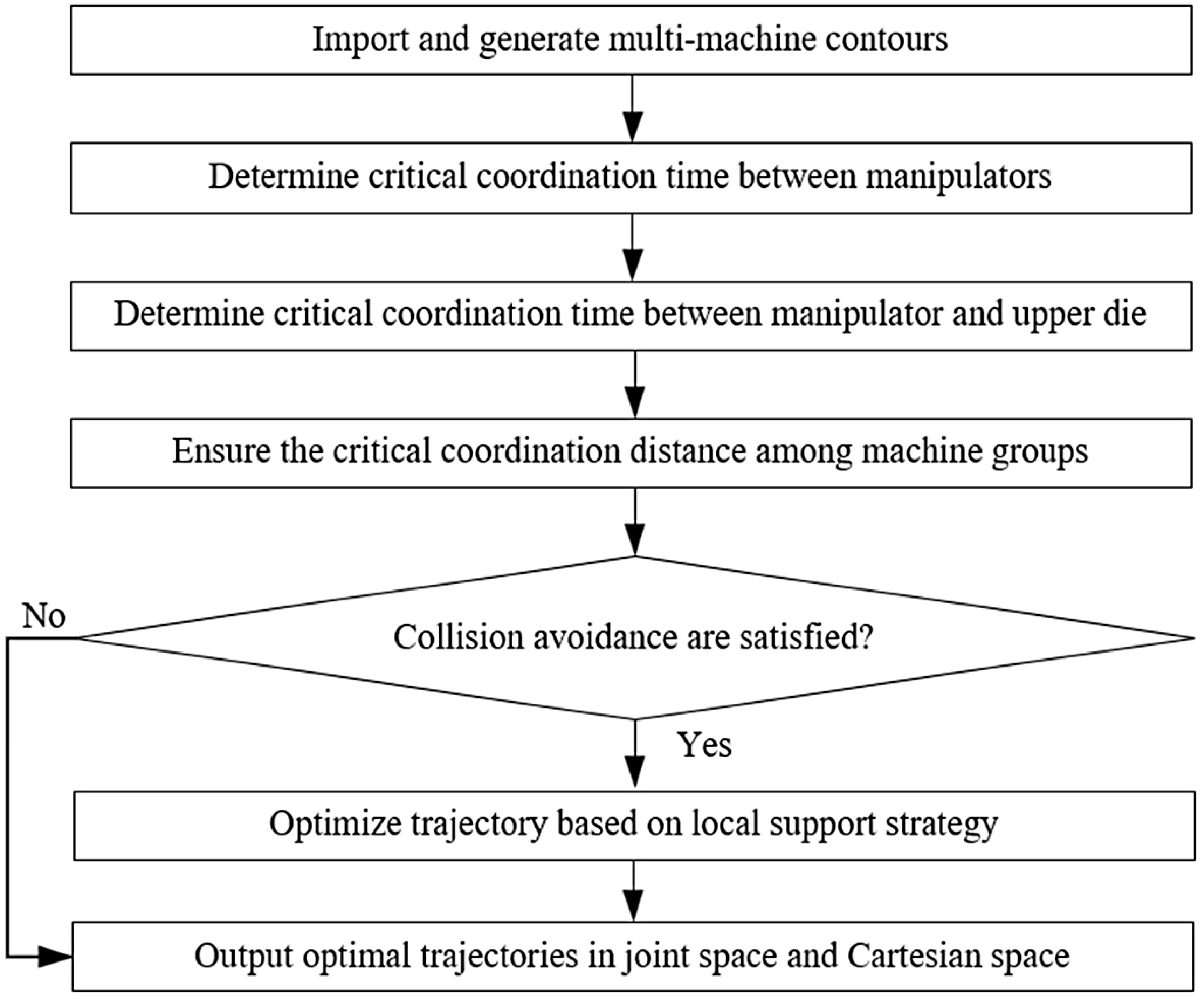
Multiple machines are prone to collision and interference in a dynamic and narrow space. Position adjustment and period optimization are common collision-free methods. But they cannot ensure the smooth transition of variable period trajectory between local support region and local optimization region. In this case, the analytical reinforcement method is proposed to fine-tune the trajectory with local support performance. Local support performance ensures the trajectory is optimized in specific local regions to prevent collision and maintain high performance. Detailed steps of the proposed method are introduced in Figure 7.
Trajectory optimization steps based on the analytical reinforcement method.

Step 1: Import and generate multi-machine contours
According to similar procedures in Figure 3, multi-machine contours such as upper die, lower die, sheet metal part, and manipulator links are imported and generated in the programming software named Python. To improve the reliability of collision detection and trajectory optimization results, the machine layout in Python is established in accordance with the actual experiment. The lower die is static, and the upper die is driven by the fixed path of the crank-link mechanism. Based on the analytical equation of forward kinematics, the position relationship of the multi-link manipulator is established. Multi-link manipulator and sheet metal part are driven by trajectories in joint space.
Step 2: Determine critical coordination time between manipulators
As shown in Figure 1, after the upper die completes the stamping in the stamping station 1, manipulator 2 needs to take out the stamped sheet metal part, then manipulator 1 places the new sheet metal part to be stamped in the stamping station 1. The two manipulators handle the sheet metal part in the same working area. If the two manipulators are not coordinated properly, unexpected collision may occur. Generally, the width of the sheet metal part is greater than that of the end-effector attached to the manipulator. If the distance between two adjacent end-effector is too small, the two sheet metal parts will be easily prone to collision.
Combined with the collision-free gradient optimization function based on the circle envelope method in Section 2.2, the gradient contour of the manipulator 2 is generated. As the crucial reference for collision detection, the gradient value g is the safety distance between manipulators 1 and 2. When the manipulator 1 enters the stamping station 1, the critical coordination time
 $\Delta$
t
m1-m2 between manipulators 1 and 2 in Figure 1 is obtained by Eq. (8). Based on Eq. (5), if g′
is less than g, collision will occur.
 \begin{equation} \Delta t_{m1-m2}={\unicode{x03A8}} _{i={\unicode{x0394}} t}\left\{g',g\right\} \end{equation}
where
 ${\unicode{x03A8}}$
is the mathematical operation shown in Eq. (9). g′
is the calculated distance obtained by Eq. (10).
 \begin{equation} {\unicode{x03A8}} _{i={\unicode{x0394}} t}\left\{g',g\right\}=\left\{\begin{array}{ll} \Delta t,&{\rm if}\ g'\geq g\ {\rm and}\ 1\leq \Delta t\leq F\left(t_{m1},\,t_{m2}\right)-1\\ {\unicode{x03A8}} _{i=\Delta t+1}\left\{g',g\right\},&{\rm if}\ g'\lt g\ {\rm and}\ 1\leq \Delta t\lt F\left(t_{m1},\,t_{m2}\right)-1\\ {\rm none},&{\rm if}\ g'\lt g\ {\rm and}\ \Delta t=F\left(t_{m1},\,t_{m2}\right)-1 \end{array}\right. \end{equation}
where t
m1 is the number of time points for manipulator 1 in stamping station 1. t
m2 is the number of time points for manipulator 2 in stamping station 1.
 $\Delta$
t is the time point, with an initial value of 1. none means that Eq. (9) has no solution. F is the mathematical operation shown in Eq. (11).
 \begin{equation} g'=F\left(\overset{F\left(t_{m1},t_{m2}\right)}{\underset{j=1}{\Lambda} }\left| f\left(r_{t_{1+j}}^{m1}\right),\,f\left(r_{t_{i+j}}^{m2}\right)\right| ,g\right) \end{equation}
where
 $\Lambda$
is the mathematical operation to find the minimum Euclidean distance between the points in two sets.
 $f(r^m_t)$
is the mathematical operation to obtain the position of the manipulator m at time t.
 \begin{equation} F\left(i,j\right)=\left\{\begin{array}{ll} i,&{\rm if}\ i\leq j\\ j,&{\rm else} \end{array}\right. \end{equation}
Step 3: Determine critical coordination time between manipulator and upper die
When the manipulator is outside the stamping station, there is no collision. Otherwise, distance calculation and collision detection are performed. Combined with the collision-free gradient optimization function based on the circle envelope method in Section 2.2, the gradient contour of the upper die is generated. Based on Eqs. (8)–(11), the critical coordination time
 $\Delta$
t
m1-u1 between the manipulator 1 and upper die 1 in Figure 1 is obtained. Similarly, the critical coordination time
 $\Delta$
t
m2-u1 between the manipulator 2 and upper die 1 in Figure 1 is also obtained.
Step 4: Ensure the critical coordination distance among machine groups
Decentralized dynamic trajectory planning between three groups A, B, and C of adjacent machines in the stamping station 1 is carried out in Steps 3 and 4. Adjacent machines in group A include manipulators 1 and 2. Adjacent machines in group B include the manipulator 1 and upper die 1. Adjacent machines in group C include the manipulator 2 and upper die 1. The corresponding critical coordination time is determined. For the trajectory planning between closed-loop machines, even if there is no collision or interference between machines in any two groups, there may still be collision or interference between machines in the remaining group. This paper assumes that there is no collision or interference between machines in groups A and C. In this case, machines in the group B are more likely to collide. If there is no collision between machines in the group B, Step 5 will be skipped out. Otherwise, the following procedures will be executed. The maximum collision time t col and the critical coordination distance d col between manipulator 1 and upper die are obtained by Eq. (12).
 \begin{equation} \begin{array}{l} \left(d_{{\rm col}},t_{{\rm col}}\right)={\unicode{x0398}} \left\langle Gro_{B}\right\rangle \\ s.t.\left(Gro_{A}\cup Gro_{C}\right)=0 \end{array} \end{equation}
where Θ is the mathematical operation to extract the maximum collision time t col and the critical coordination distance d col. Gro A, Gro B , and Gro C are shown in Eqs. (13)–(15).
 \begin{equation} Gro_{A}={\Phi} \left(\overset{t_{m2}}{\underset{j=1}{\Lambda} }\left| f\left(r_{t_{j}-\Delta t_{m1-m2}}^{m1}\right),\,f\left(r_{t_{j}}^{m2}\right)\right| ,g\right) \end{equation}
where
 ${\Phi}$
is the mathematical operation to extract the collision time set Gro
A
between manipulators 1 and 2 when the value of calculated distance is smaller than g.
 \begin{equation} Gro_{B}={\Phi} \left(\overset{t_{u1}}{\underset{j=1}{\Lambda} }\left| f\left(r_{t_{j}-\Delta t_{m1-u1}}^{m1}\right),\,f\left(r_{t_{j}}^{u1}\right)\right| ,g\right) \end{equation}
where Gro B is the collision time set between the manipulator 1 and upper die 1 when the value of calculated distance is smaller than g.
 \begin{equation} Gro_{C}={\Phi} \left(\overset{t_{u1}}{\underset{j=1}{\Lambda} }\left| f\left(r_{t_{j}-\Delta t_{m2-u1}}^{m2}\right),\,f\left(r_{t_{j}}^{u1}\right)\right| ,g\right) \end{equation}
where Gro C is the collision time set between the manipulator 2 and upper die 1 when the value of calculated distance is smaller than g.
Step 5: Optimize trajectory based on local support strategy
Based on the analytical equation of inverse kinematics, the pose of the manipulator in joint space can be adjusted by the trajectory in Cartesian space. As mentioned in Step 4, collisions can only occur between manipulator 1 and upper die 1. The structure of the high-speed flexible manipulator is shown in Figure 8. The structure diagram of the planar manipulator and its adjacent upper die is shown in Figure 9. Based on Eq. (16), the collision-free trajectory between the manipulator and the upper die at time t col is generated by the analytical reinforcement method.
 \begin{equation} \Delta \theta _{{t_{{\rm col}}}}=\arcsin \left(\frac{Y_{\min }-E_{y}}{\sqrt{\left(f_{x}\left(r_{t_{{\rm col}}}^{m1}\right)-E_{x}\right)^{2}+\left(f_{y}\left(r_{t_{{\rm col}}}^{m1}\right)-E_{y}\right)^{2}}}\right) \end{equation}
where
 $\Delta$
θ
is the adjusted pose of joint R
5. E
x
and E
y
are coordinates of joint R
6 in the horizontal and vertical directions, respectively. Y
min is the minimum coordinate of the upper die in the vertical direction.
The structure of the high-speed flexible manipulator.

Structure diagram of multi-machine coordination.

Combined with Eq. (16), the optimal pose r5′ of joint R5 is obtained by Eq. (17).
 \begin{equation} r_{5}^{\prime}=r_{5}+\Delta \theta _{{t_{{\rm col}}}} \end{equation}
where r 5 is the original pose of joint R 5.
Based on analytical equations of inverse kinematics, the optimal coordinates
 $d_{4x}^{\prime}$
,
 $d_{4y}^{\prime}$
of joint D
4 in the horizontal and vertical directions can be calculated by Eq. (18). In the vertical direction, the optimal pose
 $d_{1y}^{\prime}$
of joint D
1 and the optimal pose
 $d_{7y}^{\prime}$
of joint D
7 can be calculated by Eqs. (19) and (20), respectively.
 \begin{equation} \left\{\begin{array}{l} d_{4x}^{\prime}=E_{\mathrm{x}}-l_{5}\sin r_{5}^{\prime}\\ d_{4y}^{\prime}=E_{y}-\xi _{4}+l_{5}\cos r_{5}^{\prime} \end{array}\right. \end{equation}
where l 5 is the length of link between joints R 5 and R 6. ξ 4 is the error constant.
 \begin{equation} d_{1y}^{\prime}=d_{1y}-\xi _{1} \end{equation}
where d 1y is the original pose of joint D 1. ξ 1 is the error constant.
 \begin{equation} d_{7y}^{\prime}=d_{7y}-\xi _{7} \end{equation}
where d 7y is the original pose of joint D 7. ξ 7 is the error constant.
Based on Eqs. (18)–(20), the optimal pose
 $r_{3}^{\prime}$
of joint R
3 and the optimal pose
 $r_{2}^{\prime}$
of joint R
2 can be modified to Eqs. (21) and (22), respectively.
 \begin{align}& r_{3}^{\prime}=\arctan \left(\frac{d_{4x}^{\prime}}{d_{4y}^{\prime}-d_{7y}^{\prime}}\right) \end{align}
 \begin{align}&\,\, r_{2}^{\prime}=\arcsin \left(\frac{l_{3}\sin r_{3}^{\prime}}{l_{2}}\right) \end{align}
where l 2 is the length of link between points A and C in Figure 8. l 3 is the length of link between points B and C in Figure 8.
In order to ensure the smoothness of manipulator trajectory at the local optimization region, the probability density function F(x) of the chi-square distribution in Eq. (23) is used.
 \begin{equation} F\left(x\right)=\frac{1}{2{\Gamma} \left(n/2\right)}\left(\frac{x}{2}\right)^{\frac{n}{2}-1}e^{-\frac{1}{2}} \end{equation}
where n is the degree of freedom. The symbol
 ${\Gamma}$
of mathematical operation is shown in Eq. (24).
 \begin{equation} {\Gamma} \left(\alpha \right)=\int _{0}^{+\infty }x^{\alpha -1}e^{-x}dx \left(x\gt 0\right) \end{equation}
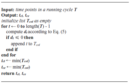
determining local optimization region

The algorithm 1 provides the procedure for determining the time interval [t cl , t ce] corresponding to the local optimization region. Combined with the local support strategy in Section 2.3, the trajectory at the local optimization region with time interval [t cl , t ce] can be further optimized. It is represented by Eq. (25).
 \begin{equation} J_{k}^{\prime}\left(x\right)=\left\{\begin{array}{l} \frac{J_{k}^{\prime}}{F\left(x\right)_{\max }}\left(F\left(x\right)-F\left(x\right)_{\min }\right),x\in \left[t_{cl},t_{ce}\right]\\ J_{k}\left(x\right), \textit{otherwise} \end{array}\right. \end{equation}
where J
k
is the pose of joint k at the local support region.
 $J_{k}^{\prime}$
is the pose of joint k at the local optimization region. t
cl
is the beginning time of the collision. t
ce
is the end time of the collision.
Step 6: Output optimal trajectories in joint space and Cartesian space
A sharp curve in the motion trajectory may lead to abrupt changes in force and acceleration. The lower the transient vibration and overshoot of the manipulator, the better the performance of the motion trajectory. In addition, the average acceleration is related to the torque, which reflects the energy consumption of the motor. To maintain the high performance of the motion trajectory, principles 1 to 3 should be satisfied.
Principle 1: There is no sharp point on the velocity curve during the continuous motion period.
Principle 2: There is no collision among machines during the continuous motion period.
Principle 3: The performance metric for the trajectory is determined by Eq. (26). When compared to the initial trajectory, the changes in the values of f 1 and f 2 in the optimal trajectory should be less than 5%.
 \begin{equation} \begin{array}{l} f_{1}=\int _{i=1}^{n_{c}}\frac{\left(t_{i-1}+t_{i}\right)a_{i}}{2}\\ f_{2}=\int _{i=1}^{n_{c}}\frac{\left(t_{i-1}+t_{i}\right)j_{i}}{2}\\ s.t. a_{\min }\leq a_{i}\leq a_{\max }\\ j_{\min }\leq j_{i}\leq j_{\max } \end{array} \end{equation}
where f 1 and f 2 are functions to measure the energy consumption and evaluate the smoothness of the trajectory, respectively. a min and j min are minimum values of acceleration and jerk, respectively. a max and j max are maximum values of acceleration and jerk, respectively. n c is the number of time points at the local optimization region.
Principle 3 will not be implemented until Principles 1 and 2 are satisfied. If Principles 1–3 are satisfied, optimal trajectories in joint space and Cartesian space can be generated. Otherwise, Steps 5 and 6 will be re-executed. The proposed method will not be terminated until the optimal trajectory satisfying Principles 1–3 is generated.
4. Case study
The planar manipulator with 5 degrees of freedom and 2 redundancies in Figure 8 is taken as the case to illustrate the proposed method. Trajectories in Cartesian and joint space can be firstly generated by the method based on the joint classification and particle swarm optimization algorithm [Reference Huang, Zhou, Yu and Wang34]. The width of sheet metal part affects the work efficiency of the manipulator. With the width diminished of sheet metal part in stamping line, the work efficiency of its corresponding manipulator improves. In this case, the trajectory performance of the leftmost manipulator is the bottleneck factor to improve the work efficiency of the stamping line. The handling period of the feeding manipulator is 4s. It is discretized into 4800 time points. The widths of sheet metal parts 1 and 2 in Figure 1 are 2.224 and 2.210 m, respectively. Based on Eqs. (8)–(11), the critical coordination time
 $\Delta$
t
m1-m2
in Eq. (8) is 1750. Similarly, the critical coordination time
 $\Delta$
t
m1-u1 in step 3 in Section 3 between manipulator 1 and upper die 1 is 800. The critical coordination time
 $\Delta$
t
m2-u1 in step 3 in section 3 between manipulator 2 and upper die 1 is 3600. The distance between manipulator 1 and upper die 1 is rapidly calculated by on collision-free gradient optimization function. Based on Eq. (12), the maximum collision time t
col
and the critical coordination distance d
col
between manipulator 1 and upper die are 2000 and 0.275m, respectively.
Horizontal operation of the link R5 in the die area can improve the work efficiency of coordination. Compared with Figure 10(a), the inclined link R5 of manipulator 1 in Figure 10(b) requires smaller space to work in die area and more efficiency. Therefore, changing the initial pose of manipulator enables efficient operation in narrow feeding scenarios. The rapid change of pose in joint space will decrease the performance of the initial trajectory and lead to increased vibration and energy consumption. The analytical reinforcement method is used to address this issue, and locally optimize the trajectory of the feeding manipulator 1. To ensure the smooth transition of the whole trajectory, the chi-square distribution in Eq. (23) is utilized and n is adjusted to 80. Combined with Eq. (25), the optimal trajectory with local support performance can be generated. The end-effector optimal trajectory in the vertical direction in Cartesian space is shown in Figure 11. Notably, units of displacement s, velocity v, acceleration a, jerk j, and time t are m, m/s, m/s 2 , m/s 3 , and s, respectively. The black and blue curve in Figure 11 represent initial trajectory and optimal trajectory of manipulator 1, respectively.
The coordination at the same moment before and after optimization.

The end-effector optimal trajectory in the vertical direction.

Similarly, the end-effector optimal trajectory in the horizontal direction in Cartesian space is shown in Figure 12. On this basis, combined with the forward kinematics and inverse kinematics equations [Reference Yu, Wang, Zhang and Zhang32], displacement-time and velocity-time curves of some typical active joints R2, D4, and R5 in joint space are shown in Figure 13. Notably, units of displacement and velocity for rotary joints are rad and rad/s, respectively.
The end-effector optimal trajectory in the horizontal direction.

The high-performance trajectories of typical active joints.

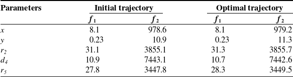
In Table I, units of f 1 and f 2 for r 2 , r 5 are rad/s2 and rad/s3, respectively. Units of f 1 and f 2 for other parameters are m/s2 and m/s3, respectively. f 1 and f 2 in the initial and optimal trajectories are approximately identical. In addition, by the continuous periodic running in Figure 14, simulation and experiment results show that there is no collision between the manipulator and adjacent machines. The optimal trajectory improves the efficiency of manipulator in the narrow feeding scenario. The consistent work efficiency between the manipulator and the whole stamping line is achieved.
The motion state of the manipulator at one moment.

f1 and f2 corresponding to initial and optimal trajectories.

5. Discussion
The section mainly discusses results obtained by analytical reinforcement method. During the multi-machine coordination in the stamping line, the manipulator may collide with the adjacent dynamic and static machines. As the stamping process advances from the leftmost stamping station to the rightmost stamping station in Figure 1, the width of the sheet metal part becomes smaller and smaller. The larger the width of sheet metal parts, the higher the collision possibility between the feeding manipulator and its adjacent machines. In this case, the trajectory performance of the leftmost manipulator is the bottleneck factor to improve the work efficiency of the stamping line. The multi-machine coordination in the stamping line is transformed into the coordination between the leftmost manipulator and its adjacent machines. Therefore, the proposed method applies to the local collision-free trajectory optimization in the progressive die stamping line, multi-station stamping line, and other similar working scenes [Reference Yu33].
Contour is a key indicator to determine whether the two machines collide. Euclidean distance equation is commonly used to obtain the shortest distance between two contours. Due to the low computational efficiency, it is easy to fail in the multiple machines with a large amount of scatter contour points. To this issue, the collision-free gradient optimization function based on the circle envelope method is proposed to improve the distance evaluation efficiency. If the shortest distance between two machines exceeds the desired value, the trajectory is commonly optimized by changing some poses in joint space based on the original intelligent trajectory optimization method [Reference Yu, Wang, Zhang and Zhang32, Reference Huang, Zhou, Yu and Wang34]. But it is prone to singularities, solving failures, increasing solving time, and other inefficiencies. Based on the existing multi-machine coordination trajectory [Reference Yu, Wang, Zhang and Zhang32], the proposed analytical reinforcement method can rapidly generate the expected trajectory.
The work efficiency of the feeding manipulator is generally significantly higher than that of the multi-machine coordination in the whole stamping line. To ensure the continuous running of multiple machines in the stamping line, the actual running speed of the feeding manipulator out of the stamping station in Figure 1 is slow [Reference Yu, Zhou and Huang28]. By the proposed analytical reinforcement method, the consistent work efficiency between the original manipulator and the whole stamping line is achieved by generating smooth trajectory with local support performance.
6. Conclusions
In this paper, collision-free trajectory with local support performance is investigated for the emergency collision avoidance of the coordinated manipulator in the flexible stamping line. Main conclusions are listed below.
-
1. Combined with the analytical equation of inverse kinematics, the analytical reinforcement method is proposed to generate collision-free trajectories with local support performance. It can improve the trajectory optimization efficiency of the multi-machine coordination.
-
2. The probability density function of the chi-square distribution is used to optimize the trajectory smoothness. There is no sharp point in the optimal displacement and velocity curves. Compared with that in the initial trajectory, the variation of f 1 and f 2 in the optimal trajectory is less than 2%.
-
3. After local emergency collision avoidance, simulation and experiments show that the feeding manipulator can run continuously. And the work efficiency of the whole stamping line is consistent with that of the feeding manipulator.
The scope of this study is limited to the multi-machine coordination of planar manipulators. It is a challenge to calculate the minimum distances between spatial manipulator and multi-machine. The issue of multi-machine coordination of spatial manipulators is an intriguing one which could be usefully explored in further research.
Data availability
The authors do not have permission to share data.
Author contribution
Xingyu Zhang: Formal analysis, Writing-original draft, Investigation. Luchuan Yu: Writing-review & editing, Supervision. Shenquan Huang: Conceptualization, Supervision. Youzhi Zhang: Investigation.
Competing interests
The authors declare that they have no known competing financial interests or personal relationships that could have appeared to influence the work reported in this paper.
Financial support
This work was supported by National Natural Science Foundation of China (grant number 52305549); and Innovation Ability Improvement Project of Science and Technology Small and Medium Enterprises in Shandong Province (grant number 2024TSGC0628).