



1. Introduction
The formation of structures in turbulent flows is ubiquitously observed in nature, for example in atmospheric flows or oceans. In two-dimensional hydrodynamic turbulence, the structure formation process is associated with the inverse cascade of kinetic energy, transferring this quantity from smaller to ever larger spatial scales. This well-known phenomenon has already been predicted in the seminal papers of Kraichnan (Reference Kraichnan1967), Leith (Reference Leith1968) and Batchelor (Reference Batchelor1969) (KLB) and observed in numerous simulations (e.g. Lilly Reference Lilly1971; Frisch & Sulem Reference Frisch and Sulem1984; Maltrud & Vallis Reference Maltrud and Vallis1993; Boffetta & Musacchio Reference Boffetta and Musacchio2010) and experiments (e.g. Paret & Tabeling Reference Paret and Tabeling1998; Rutgers Reference Rutgers1998; Chen et al. Reference Chen, Ecke, Eyink, Rivera, Wan and Xiao2006). We have chosen this physical system for the present work because it allows us to study naturally emergent coherence typically appearing in the form of structurally rather simple vortices or combinations of those. These vortical structures are embedded in a statistically isotropic and turbulent two-dimensional flow which is conveniently accessible to direct numerical simulation (DNS) and measurement.
An intuitive and commonly accepted defining characteristic of coherence is persistence for a finite time, which leaves room for more detailed specification. A mathematically unique definition would not only be beneficial for fluid mechanics research but also for related disciplines such as astrophysics. There, the problem of the non-universality regarding vortex identification has been pointed out by Canivete Cuissa & Steiner (Reference Canivete Cuissa and Steiner2020) and Yadav, Cameron & Solanki (Reference Yadav, Cameron and Solanki2021) with respect to studies of the solar atmosphere.
A number of methods for the detection of coherent structures exist that are often built on different specifications of coherence. In fact, most of the comparative studies in the literature focus on a specific class of coherence specification, e.g. Jeong & Hussain (Reference Jeong and Hussain1995) studied various vortex criteria, Hadjighasem et al. (Reference Hadjighasem, Farazmand, Blazevski, Froyland and Haller2017) compared different techniques for Lagrangian coherent structure (LCS) identification and Taira et al. (Reference Taira, Brunton, Dawson, Rowley, Colonius, McKeon, Schmidt, Gordeyev, Theofilis and Ukeiley2017) discussed numerous mode decomposition methods. A comparison and meaningful evaluation of different detection strategies and of their respective coherence specification requires fiducial physical properties of the considered flow which can be related to the detected structures.
In the present work, we consider three coherence detection schemes, two vorticity based and one of Lagrangian type, that use the Okubo–Weiss (OW) criterion (Okubo Reference Okubo1970; Weiss Reference Weiss1991), the vorticity magnitude (VM) and the finite-time Lyapunov exponent (FTLE) field determining LCSs (Haller & Yuan Reference Haller and Yuan2000; Haller Reference Haller2015). We compare the detection results by investigating the physical properties of the coherent and the residual (non-coherent) structures in the two-dimensional turbulent system.
The work of Ouellette (Reference Ouellette2012) follows a similar approach, which has led to several experimental studies (see Liao & Ouellette Reference Liao and Ouellette2013; Kelley, Allshouse & Ouellette Reference Kelley, Allshouse and Ouellette2013). The low Reynolds numbers attained in these two-dimensional experiments ( $Re = 185$ (Liao & Ouellette Reference Liao and Ouellette2013) and
 $Re = 220$ (Kelley et al. Reference Kelley, Allshouse and Ouellette2013)), however, do not allow for, e.g., an adequate investigation of cross-scale turbulent interactions in the framework of the KLB similarity ansatz. This motivates the use of DNSs in the present investigation.
More specifically, we consider spectral nonlinear cross-scale fluxes of energy, as well as their scale-filtered correspondents in configuration space. We also compare with previous results based on a multi-scale gradient (MSG) ansatz and employ a recently proposed vortex scaling phenomenology for two-dimensional Navier–Stokes turbulence (Burgess & Scott Reference Burgess and Scott2017, Reference Burgess and Scott2018) which applies dimensional arguments to impose physically motivated constraints onto coherent vortices. The results obtained by these theoretical approaches serve as physical reference points for the comparison of structure detection techniques and the interpretation of their results in relation to the inverse turbulent cascade of energy.
This paper is structured as follows. Section 2 presents the decomposition of the flow into coherent and residual contributions. Section 3 briefly introduces coherent structure specifications. Section 4 describes the applied diagnostics and theoretical concepts. Section 5 presents numerical methods and the parameters used for simulations and analysis. The main results are presented in § 6. A conclusion is given in § 7.
2. Physical model and flow decomposition
We consider Navier–Stokes turbulence on a two-dimensional  $2{\rm \pi}$-periodic square of size
 $A$ governed by the differential equations
 $$\begin{gather} \partial_t \boldsymbol{u} + (\boldsymbol{u} \boldsymbol{\cdot} \boldsymbol{\nabla}) \boldsymbol{u} ={-}\boldsymbol{\nabla} p + \nu \nabla^2 \boldsymbol{u}, \end{gather}$$
 $$\begin{gather}\boldsymbol{\nabla} \boldsymbol{\cdot} \boldsymbol{u} = 0, \end{gather}$$
where  $\boldsymbol {u} = (u_x, u_y)$,
 $p$ and
 $\nu$ are the velocity, pressure and kinematic viscosity, respectively. The kinetic energy per unit mass
 $E = (1/2A) \int _A \boldsymbol {u}^2 \,{\rm d}A$ and the enstrophy
 $\varOmega = (1/2A) \int _A \omega ^2 \,{\rm d}A$ defined with the vorticity
 $\omega = \partial _x u_y - \partial _y u_x$, are inviscid invariants in a two-dimensional configuration. The kinetic energy exhibits an inverse cascade, transferring energy from small to large length scales, in contrast to the enstrophy, which exhibits a direct cascade.
We employ a decomposition of the total vorticity field into a coherent part,  $\omega _c$, and a residual/incoherent contribution,
 $\omega _r$, (cf. Ohkitani Reference Ohkitani1991) to carry out the analysis of different schemes for coherence detection (cf. § 3):
 $$\begin{gather} \omega = \omega_c + \omega_r, \end{gather}$$
 $$\begin{gather}\omega_c(\boldsymbol{x}) = \begin{cases} \omega(\boldsymbol{x}), & \epsilon(\boldsymbol{x}) \geq \epsilon_{thr}, \\ 0, & \epsilon(\boldsymbol{x}) < \epsilon_{thr}, \end{cases} \end{gather}$$
 $$\begin{gather}\omega_r(\boldsymbol{x}) = \begin{cases} 0, & \epsilon(\boldsymbol{x}) \geq \epsilon_{thr}, \\ \omega(\boldsymbol{x}), & \epsilon(\boldsymbol{x}) < \epsilon_{thr}. \end{cases} \end{gather}$$
Based on the particular specification of coherence, a physical characteristic of the flow,  $\epsilon (\boldsymbol {x})$, serves as an indicator of this property, turning the detection into a thresholding procedure with a fixed threshold,
 $\epsilon _{thr}$. In order to improve comparability of different detection schemes, it is important to gauge their thresholds with respect to a physical property of the flow (see § 3.4). Technical details of the decomposition are pointed out in Appendix A.1. The coherent velocity field,
 $\boldsymbol {u}_c = (u_{c,x}, u_{c,y})$, and the residual velocity
 $\boldsymbol {u}_r = (u_{r,x}, u_{r,y})$, are approximated by inverting
 $\boldsymbol {\omega }_{c/r}=\boldsymbol {\nabla }\times \boldsymbol {u}_{c/r}$ in Fourier space, a procedure symbolically represented by the operator
 $\boldsymbol {\nabla }\times \nabla ^{-2}$, which similarly has been employed in several related works (see Benzi et al. Reference Benzi, Paladin, Patarnello, Santangelo and Vulpiani1986; Benzi, Patarnello & Santangelo Reference Benzi, Patarnello and Santangelo1988; Borue Reference Borue1994; Okamoto et al. Reference Okamoto, Yoshimatsu, Schneider, Farge and Kaneda2007; Yoshimatsu et al. Reference Yoshimatsu, Kondo, Schneider, Okamoto, Hagiwara and Farge2009; Vallgren Reference Vallgren2011; Burgess & Scott Reference Burgess and Scott2018):
 \begin{equation} \left. \begin{aligned} \boldsymbol{u}_{c/r} & ={-}\boldsymbol{\nabla} \times (\nabla^{{-}2} \boldsymbol{\omega}_{c/r}),\\ \boldsymbol{u} & = \boldsymbol{u}_{c} + \boldsymbol{u}_{r}. \end{aligned} \right\} \end{equation}
This enables straightforward access to various decomposed turbulent fields and related quantities such as the Fourier spectrum of kinetic energy per unit mass. It is defined as  $E(k) = \sum _k | \hat {\boldsymbol {u}}(\boldsymbol {k}) |^2 / 2$ with the wavevector
 $\boldsymbol {k}=(k_x,k_y)$ and for the respective length scale
 $\ell \sim k^{-1}$. Fourier-transformed quantities are denoted by ‘
 $\unicode{x005E} $’ and the sum over all wavevectors located on a wavenumber shell,
 $k \leq | \boldsymbol {k} | < k+1$, is indicated as
 $\sum _k$. According to the KLB phenomenology, the spectrum possesses scaling properties for the inverse kinetic energy and direct enstrophy cascade ranges, which are
 $$\begin{gather} E(k) \sim \epsilon_I^{2/3} k^{{-}5/3}, \quad k \ll k_f, \end{gather}$$
 $$\begin{gather}E(k) \sim \eta_I^{2/3} k^{{-}3}, \quad k \gg k_f, \end{gather}$$
with  $k_f$ the forcing wavenumber at which energy and enstrophy are injected with an injection rate
 $\epsilon _I$ or
 $\eta _I = k_f^2 \epsilon _I$, respectively. Here, we are interested in a decomposition of the kinetic energy spectrum as
 \begin{equation} E(k) = E_{c}(k) + E_{r}(k) + E_{cr}(k), \end{equation}
where  $E_{c}(k) = \sum _k | \hat {\boldsymbol {u}}_c(\boldsymbol {k}) |^2 / 2$ and
 $E_{r}(k) = \sum _k | \hat {\boldsymbol {u}}_r(\boldsymbol {k}) |^2 / 2$ are associated to spectral contributions from purely coherent and residual regions, respectively, and
 $E_{cr}(k) = \sum _k \mathrm {Re}[\hat {\boldsymbol {u}}^{*}_c(\boldsymbol {k}) \boldsymbol {\cdot } \hat {\boldsymbol {u}}_r(\boldsymbol {k})]$ the spectrum resulting from mixed contributions of coherent and residual parts, with ‘
 ${ }^{*}$’ denoting the complex conjugate.
In the following, we introduce the identification schemes considered for  $\epsilon (\boldsymbol {x})$ in (2.4) and (2.5) and the choice of the corresponding threshold values
 $\epsilon _{thr}$.
3. Coherence specifications
In general, schemes for the detection of coherent structures can be grouped into several categories including threshold methods, modal decomposition methods such as proper orthogonal decomposition (POD) (Holmes et al. Reference Holmes, Lumley, Berkooz and Rowley2012), dynamic mode decomposition (DMD) (Rowley et al. Reference Rowley, Mezić, Bagheri, Schlatter and Henningson2009; Schmid Reference Schmid2010) or spectral proper orthogonal decomposition (SPOD) (Towne, Schmidt & Colonius Reference Towne, Schmidt and Colonius2018) and wavelet methods (see Okamoto et al. Reference Okamoto, Yoshimatsu, Schneider, Farge and Kaneda2007; Yoshimatsu et al. Reference Yoshimatsu, Kondo, Schneider, Okamoto, Hagiwara and Farge2009; Farge & Schneider Reference Farge and Schneider2015). In this work, we focus on threshold methods, in particular the approaches based on the OW criterion (Okubo Reference Okubo1970; Weiss Reference Weiss1991), the VM and the LCSs (Haller & Yuan Reference Haller and Yuan2000; Haller Reference Haller2015). These schemes are straightforwardly employed using equations (2.4) and (2.5). The thresholds for the VM and for the LCS-based structure detection are chosen with the help of vortex scaling (see § 3.4).
3.1. Okubo–Weiss criterion (OW) $/Q$-criterion

A frequently applied quantity for structure identification is the Eulerian velocity gradient tensor  $\boldsymbol {\nabla } \boldsymbol {u}$, which is often investigated in decomposed form
 $\boldsymbol {\nabla } \boldsymbol {u} = \boldsymbol{\mathsf{S}} + \boldsymbol{\mathsf{W}}$, with
 $\boldsymbol{\mathsf{S}} = (\boldsymbol {\nabla } \boldsymbol {u} + (\boldsymbol {\nabla } \boldsymbol {u})^\textrm {T})/2$ the symmetric strain-rate tensor and
 $\boldsymbol{\mathsf{W}} = (\boldsymbol {\nabla } \boldsymbol {u} - (\boldsymbol {\nabla } \boldsymbol {u})^\textrm {T})/2$ the skew-symmetric spin tensor. The usage of invariants of
 $\boldsymbol {\nabla } \boldsymbol {u}$, e.g. the eigenvalues or the trace, and of its tensor decomposition have led to numerous identification schemes (see e.g. Hunt, Wray & Moin Reference Hunt, Wray and Moin1988; Chong, Perry & Cantwell Reference Chong, Perry and Cantwell1990; Jeong & Hussain Reference Jeong and Hussain1995; Hua Reference Hua1998; Zhou et al. Reference Zhou, Adrian, Balachandar and Kendall1999; Chakraborty, Balachandar & Adrian Reference Chakraborty, Balachandar and Adrian2005). However, all of these methods face the problem of objectivity (Haller Reference Haller2005; Haller et al. Reference Haller, Hadjighasem, Farazmand and Huhn2016), i.e. they lack invariance under certain transformations of the frame of reference which combine rotation and translation. Thus, for the sake of simplicity, we restrict ourselves to the well-known
 $Q$-criterion (Hunt et al. Reference Hunt, Wray and Moin1988), whose two-dimensional equivalent resembles the OW criterion. It is defined as
 \begin{equation} Q = \tfrac{1}{2}
(\left| \boldsymbol{\mathsf{W}} \right|^2 - \left| \boldsymbol{\mathsf{S}} \right|^2) = \tfrac{1}{2} ( \tfrac{1}{2} \omega^2
- \left| \boldsymbol{\mathsf{S}} \right|^2 ),
\end{equation}
where for  $Q > 0$ vortex dominated/elliptical regions and for
 $Q < 0$ strain dominated/ hyperbolic regions are detected. Thus,
 $\epsilon (\boldsymbol {x}) = Q(\boldsymbol {x})$ and
 $\epsilon _{thr}=0$ are set in (2.4) and (2.5).
3.2. Vorticity magnitude
Coherent structures in two-dimensional flows are often most clearly visible in the spatial distribution of the vorticity. Thus, an intuitive approach is to set  $\epsilon (\boldsymbol {x}) = | \omega (\boldsymbol {x}) |$ in (2.4) and (2.5). Furthermore, the vorticity is closely connected to the Lagrangian-averaged vorticity deviation (LAVD) method (Haller et al. Reference Haller, Hadjighasem, Farazmand and Huhn2016), which is an objective detection criterion.
3.3. Lagrangian coherent structures
LCSs take the evolution of the flow field into account by determining the pair-dispersion characteristic of passively advected Lagrangian tracers (Haller & Yuan Reference Haller and Yuan2000; Haller Reference Haller2015). Thus, they reveal structures in the flow, which are neither captured by the vorticity  $\omega$ nor variants of the velocity gradient tensor
 $\boldsymbol {\nabla } \boldsymbol {u}$. To this end, the flowmap
 $\boldsymbol {F}_{t_0}^{t}(\boldsymbol {x}_0) = \boldsymbol {x}(t;t_0,\boldsymbol {x}_0)$ is considered, with
 $\boldsymbol {x}_0 = (x_0,y_0)$ the initial position at time
 $t_0$. The detection of LCSs can be realised by determining the FTLE field which is given by
 \begin{equation} \varLambda_{t_0}^{t}(\boldsymbol{x}_0) = \frac{1}{T_{eddy}} \log \sqrt{\lambda^C_2(\boldsymbol{x}_0)}, \end{equation}
with  $\lambda ^C_{2}$ the largest eigenvalue of the Cauchy–Green strain tensor
 $\boldsymbol{\mathsf{C}}_{t_0}^t(\boldsymbol {x}_0) = [ \boldsymbol {\nabla } \boldsymbol {F}_{t_0}^t(\boldsymbol {x}_0) ]^\textrm {T} \boldsymbol {\nabla } \boldsymbol {F}_{t_0}^t(\boldsymbol {x}_0)$. The FTLE is interpreted as a local measure of stretching and can be calculated forward and backward in time. Thus, the values are set to
 $\epsilon (\boldsymbol {x}) = \varLambda _{t_0}^{t_0+T_{eddy}}(\boldsymbol {x})$ for the forward-in-time and
 $\epsilon (\boldsymbol {x}) = \varLambda _{t_0}^{t_0-T_{eddy}}(\boldsymbol {x})$ for the backward-in-time case. Please note, that for the FTLE case the roles of
 $\omega _c$ and
 $\omega _r$ are switched in (2.4) and (2.5), meaning that small FTLE values correspond to coherent regions, in contrast to the VM
 $| \omega (\boldsymbol {x}) |$. This is because large FTLE values isolate coherent regions as illustrated in figure 4(c,d). To the best of the authors’ knowledge no condition exists for the flowmap integration time. Hence, we suggest setting it to the large-eddy turnover time
 $T_{eddy}$ according to § 5, which is typically the longest characteristic correlation time scale of the system. Further numerical details for the FTLE calculation are discussed in Appendix A.2.
Although more refined LCS approaches exist, for our purposes the FTLE yields sufficient insight into the flow physics, as high-valued FTLE regions, which are visually perceived as sharp ridges in the flow, are supposed to materially separate dynamically distinct domains with different transport characteristics. For example, these domains mark areas of zero cross-scale energy fluxes in low-Reynolds-number systems (cf. Kelley et al. Reference Kelley, Allshouse and Ouellette2013). Furthermore, forward-in-time FTLE (f-FTLE) ridges are associated with repelling LCSs and backward-in-time FTLE (b-FTLE) ridges to attracting LCSs, indicating stable and unstable manifolds in the flow in the sense of dynamical systems theory.
3.4. Determining the threshold: vortex scaling
Two of the three detection schemes considered here include free threshold parameters which complicate a meaningful comparison of the detection methods and the physical interpretation of the detection results. In order to achieve comparability between the three coherence specifications, the VM and LCS schemes are gauged by making use of the above-mentioned vortex scaling phenomenology.
This model, which we briefly summarise here for completeness, provides a physically motivated diagnostic signature which we use as a reference for the highly non-trivial threshold choice of  $\epsilon _{thr}$ in (2.4) and (2.5). The phenomenology characterises coherent structures by their vortex area
 $A$ in configuration space instead of the classical wavenumber dependence in Fourier space. Therefore, a time-dependent vortex number density distribution
 $n(A,t)$ is defined, which yields the number of coherent vortices per unit area for a certain vortex area
 $A$ at time
 $t$. The model is based on the first three moments of
 $n\overline {\omega _v^2}$ with the vortex intensity
 $\overline {\omega _v^2}$. They are the vortex energy
 $E_v$, vortex enstrophy
 $Z_v$ and vortex number
 $N_v$, respectively. All three quantities are assumed to be approximately conserved during the spatial growth of an ‘average’ vortex of area
 $A$. The number density is anticipated to follow a power law
 $t^{\alpha _i} A^{-r_i}$ with exponents
 $\alpha _i$ and
 $r_i$ determined via the conservation of
 $E_v$,
 $Z_v$ and
 $N_v$. The range of areas is divided into a thermal bath regime
 $A_f \leq A < A_{-}$, an intermediate scaling regime
 $A_{-} < A < A_{+}$ and a front of the vortex population
 $A_{+} < A \leq A_{max}$, respectively, where
 $A_{-}$ and
 $A_{+}$ are transitional areas,
 $A_f$ the forcing-scale area and
 $A_{max}$ the maximum vortex area.
In this model, the thermal bath is associated with the equilibration of the flow with the continuous forcing, which injects energy at a constant rate generating small-scale vorticity. This leads to an  $A$-independent flux of
 $E_v$ in
 $A$-space. The intermediate scaling regime consists of a self-similar distribution of vortex sizes. It is assumed that the enstrophy lost through filament shedding during merger and aggregation processes is replaced by the enstrophy injection such that the vortex enstrophy
 $Z_v$ is also approximately conserved. In the front regime, vortices are expected to be large and distant from each other, such that merging events rarely occur. Thus, approximately conserving the vortex number
 $N_v$. Based on these conservation assumptions, the scaling laws of the number density for varying area regimes are derived as (see Burgess & Scott Reference Burgess and Scott2017, Reference Burgess and Scott2018)
 \begin{equation} n(A,t) \sim \begin{cases} A^{{-}3}, & A_f \leq A < A_{-}, \\ t^{{-}1} A^{{-}1}, & A_{-} < A < A_{+}, \\ t^{5} A^{{-}6}, & A_{+} < A \leq A_{max}. \end{cases} \end{equation}
We take the best achievable agreement with the three regime subdivision (3.3) as a reference to gauge the threshold values in (2.4) and (2.5). Please note that this qualitative level of agreement mainly relies on the assumption that the emergence and the evolution of coherence are asymptotically self-similar for sufficiently large scale-separation between the regions of the forcing and the large scales of the system under consideration. This can only be fulfilled up to a rather modest approximate level in turbulence DNS. In the present work, the scaling exponents are considered relative to each other. Thus, their absolute numerical values are not of principal importance to the investigation. They are nevertheless mentioned above for completeness.
4. Diagnostic methods for the inverse cascade
The inverse cascade of kinetic energy corresponds to a cross-scale energy flux of which we distinguish coherent and residual contributions from three perspectives: (i) spectrally in Fourier space, (ii) scale-filtered in configuration space which combines the aspects of spatial scale and position and (iii) via a MSG approach (Eyink Reference Eyink2006b) which adds scale locality and the differentiation between involved physical processes.
4.1. Spectral flux
The temporal evolution of the energy spectrum is straightforwardly obtained from the Navier–Stokes equations (2.1) and (2.2) as
 \begin{equation} \partial_t E(k) + T(k) = D(k) + F(k), \end{equation}
with the nonlinear transfer term  $T(k) = \sum _k \mathrm {Re} [\hat {\boldsymbol {u}}^{*}(\boldsymbol {k}) \boldsymbol {\cdot } \widehat {(\boldsymbol {u} \boldsymbol {\cdot } \boldsymbol {\nabla } \boldsymbol {u})}(\boldsymbol {k})]$. Kinetic energy is provided to the flow by a forcing term
 $+\boldsymbol {f}_u$ on the right-hand side of the Navier–Stokes momentum balance (2.1). Thus, the energy source term is determined as
 $F(k) = \sum _k \mathrm {Re}[ \hat {\boldsymbol {u}}^{*}(\boldsymbol {k}) \boldsymbol {\cdot } \hat {\boldsymbol {f}}_u(\boldsymbol {k})]$, which is equivalent to the energy injection rate
 $\epsilon _I$ when summed over all Fourier wavenumbers. In order to allow for a statistically stationary state, kinetic energy accumulating at the largest length scales of the flow due to the inverse cascade has to be continuously extracted from the system. For this purpose a large-scale damping term
 $-d_{\alpha } \boldsymbol {u}$ is added to the right-hand side of (2.1). The energy sink
 $D(k) = D_{\nu }(k) + D_{\alpha }(k)$ is split into two dissipative contributions, where
 $D_{\nu }(k) = -2 \nu k^2 E(k)$ is the viscous dissipation active on small length scales and
 $D_{\alpha }(k) = -2 d_{\alpha } E(k)$ introduces friction active on large length scales. These terms are equivalent to the energy dissipation rate on viscous scales
 $\epsilon _{\nu }$ and on large scales
 $\epsilon _{\alpha }$, respectively, when summed over all wavenumbers. Details on the numerical implementation of
 $+\boldsymbol {f}_u$ and
 $-d_{\alpha } \boldsymbol {u}$ are given in the text around equation (5.1) in § 5.
The spectral cross-scale energy flux  $Z(k)$ is obtained by summing the transfer term over consecutive shells labelled by their characteristic wavenumber radius, k′′:
 \begin{equation} Z(k) = \sum_{k'=0}^k T(k') = \sum_{k'=0}^k \sum_{k''} \mathrm{Re}[\hat{\boldsymbol{u}}^{*}(\boldsymbol{k}) \boldsymbol{\cdot} \widehat{(\boldsymbol{u} \boldsymbol{\cdot} \boldsymbol{\nabla} \boldsymbol{u})}(\boldsymbol{k})], \end{equation}
and corresponds to the flux of energy from scales smaller than  $k$ to scales larger than
 $k$. The influence of the coherent and residual contributions with regard to the cascade mechanism is measured by the decomposition
 $$\begin{gather} Z(k) = \sum_{\alpha,\beta,\gamma \in \{c,r\}} Z_{\alpha,\beta,\gamma}(k), \end{gather}$$
 $$\begin{gather}Z_{\alpha,\beta,\gamma}(k) = \sum_{k'=0}^k T_{\alpha,\beta,\gamma}(k') = \sum_{k'=0}^k \sum_{k''} \mathrm{Re}[\hat{\boldsymbol{u}}_{\alpha}^{*}(\boldsymbol{k}) \boldsymbol{\cdot} \widehat{(\boldsymbol{u}_{\beta} \boldsymbol{\cdot} \boldsymbol{\nabla} \boldsymbol{u}_{\gamma})}(\boldsymbol{k})], \end{gather}$$
which results in eight independent flux contributions. We investigate the homogeneous fluxes originating from purely coherent  $Z_{c,c,c}(k)$ and residual components
 $Z_{r,r,r}(k)$, and the mixed flux arising through coherent–residual interactions as
 $Z_{cr}(k) = Z(k) - Z_{c,c,c}(k) - Z_{r,r,r}(k)$.
4.2. Spatial flux distribution
A complementary formulation of the cross-scale energy flux which captures its local structure in configuration space and which enables a detailed analysis regarding its spatial distribution is obtained by a scale-filter approach (cf. e.g. Ouellette Reference Ouellette2012). For the  $i$th component of the velocity vector the filter operation at a length scale
 $\ell$ is given by
 \begin{equation} \bar{u}_i(\boldsymbol{x}) = \int G_{\ell}(\boldsymbol{r}) u_i(\boldsymbol{x}+\boldsymbol{r}) \,\mathrm{d}^2 \boldsymbol{r}, \end{equation}
where we choose  $G_{\ell }$ as a smooth, non-negative, spatially well-localised filter kernel with unit integral. Because we are interested in the spatial distribution of the cross-scale flux, the locality aspect of the filter is crucial for the accurate localisation of flux contributions in configuration space. Hence, in this work we employ a Gaussian filter:
 $\hat {G}_{\ell }(\boldsymbol {k})=\exp (-k^2 {\ell }^2/24)$ to achieve sufficient filter locality in Fourier space as well as in configuration space. The temporal evolution of the filtered kinetic energy,
 $\bar {E} = | \bar {\boldsymbol {u}} |^2/2$, is given by (see Pope Reference Pope2000)
 \begin{equation} \partial_t \bar{E} + \partial_i \bar{q}_i ={-}\bar{\epsilon}_{\nu} - \bar{Z}, \end{equation}
with  $\partial _i$ the partial derivative of the
 $i$th component, where we use the Einstein summation convention. In addition,
 $\bar {q}_i = \bar {u}_i \bar {E} + \bar {u}_j (\bar {p} \delta _{ij} + \bar {\tau }_{ij} - 2 \nu \bar {S}_{ij})$ contains the nonlinear spatial transport and the viscous dissipation of the filtered large-scale kinetic energy with
 $\delta _{ij}$ the Kronecker delta function,
 $\bar {\epsilon }_{\nu } = 2 \nu \bar {S}_{ij} \bar {S}_{ij}$ the viscous dissipation from the filtered velocity field, and
 $\bar {Z} = - \bar {S}_{ij} \bar {\tau }_{ij}$ the spatial cross-scale flux term representing the exchange of kinetic energy between the known filtered fields and the fluctuations which have been depleted by the filter operation in the filtered numerical system. The flux term is an inner product of the (filtered) strain-rate tensor
 $\bar {S}_{ij} = (\partial _j \bar {u}_{i} + \partial _i \bar {u}_{j})/2$ and the subgrid stress tensor
 $\bar {\tau }_{ij} = \overline {u_i u_j} - \bar {u}_i \bar {u}_j$, that expresses the stresses exerted by the depleted fluctuations. Please note that we are referring to the deviatoric (trace-free) stress term
 $\mathring {\bar {\boldsymbol {\tau }}} = \bar {\boldsymbol {\tau }} - (1/2) tr(\bar {\boldsymbol {\tau }}) \mathbb {I}$, with
 $tr$ the trace operator and
 $\mathbb {I}$ the unit matrix. For the remainder we write
 $\bar {\boldsymbol {\tau }}$ instead of
 $\mathring {\bar {\boldsymbol {\tau }}}$. The production term
 $\bar {Z}$ is equally understood as a spatial cross-scale flux term. Note that choosing a sharp spectral filter instead of a smooth Gaussian filter will lead to the equality between the spatial average of the production term and the spectral flux in (4.2) as
 $\langle \bar {Z}(\boldsymbol {x}) \rangle = Z(k=2{\rm \pi} /\ell )$, if the wavenumber
 $k$ is chosen according to the filtering length scale
 $\ell$.
The strain-rate and stress tensor are further decomposed into coherent, residual and mixed contributions
 \begin{equation} \bar{Z}(\boldsymbol{x}) = \sum_{\alpha,\beta,\gamma \in \{ c, r \}} \bar{Z}_{\alpha,\beta,\gamma}(\boldsymbol{x}) = \sum_{\alpha,\beta,\gamma \in \{ c, r \}} \bar{\boldsymbol{\mathsf{S}}}_{\alpha} : \bar{\boldsymbol{\tau}}_{\beta,\gamma}, \end{equation}
with  $\bar {\boldsymbol{\mathsf{S}}}_{\alpha } = (\boldsymbol {\nabla } \bar {\boldsymbol {u}}_{\alpha } + (\boldsymbol {\nabla } \bar {\boldsymbol {u}}_{\alpha })^\textrm {T})/2$ and
 $\bar {\boldsymbol {\tau }}_{\beta,\gamma } = \overline {\boldsymbol {u}_{\beta } \boldsymbol {u}_{\gamma }} - \bar {\boldsymbol {u}}_{\beta } \bar {\boldsymbol {u}}_{\gamma }$. We propose the following three-part decomposition:
 \begin{align} \bar{Z}(\boldsymbol{x}) ={-}\bar{\boldsymbol{\mathsf{S}}} : \bar{\boldsymbol{\tau}} = & \underbrace{-\bar{\boldsymbol{\mathsf{S}}}_c : \bar{\boldsymbol{\tau}}_{c,c}}_{\bar{Z}_c(\boldsymbol{x})} \underbrace{-\bar{\boldsymbol{\mathsf{S}}}_r : \bar{\boldsymbol{\tau}}_{r,r}}_{\bar{Z}_r(\boldsymbol{x})} \nonumber\\ & \underbrace{-\bar{\boldsymbol{\mathsf{S}}}_c : \bar{\boldsymbol{\tau}}_{r,r} -\bar{\boldsymbol{\mathsf{S}}}_r : \bar{\boldsymbol{\tau}}_{c,c} -\bar{\boldsymbol{\mathsf{S}}}_c : (\bar{\boldsymbol{\tau}}_{c,r} + \bar{\boldsymbol{\tau}}_{r,c}) -\bar{\boldsymbol{\mathsf{S}}}_r : (\bar{\boldsymbol{\tau}}_{c,r} + \bar{\boldsymbol{\tau}}_{r,c})}_{\bar{Z}_{cr}(\boldsymbol{x})}, \end{align}
where  $\bar {Z}_c(\boldsymbol {x})$ consists of purely coherent and
 $\bar {Z}_r(\boldsymbol {x})$ of purely residual contributions, and
 $\bar {Z}_{cr}(\boldsymbol {x})$ is the flux contribution originating from mixed interactions.
Because the spatial cross-scale flux consists of an inner product of two tensors, the analysis of angle alignments between tensor eigenframes is possible. Thus, a polar decomposition leads to the following expression for the total and decomposed fluxes (see Eyink Reference Eyink2006b; Fang & Ouellette Reference Fang and Ouellette2016):
 $$\begin{gather} \bar{Z}(\boldsymbol{x}) ={-}2 \bar{\sigma}(\boldsymbol{x}) \bar{\lambda}(\boldsymbol{x}) \cos(2 \delta \bar{\theta}(\boldsymbol{x})), \end{gather}$$
 $$\begin{gather}\bar{Z}_{c/r}(\boldsymbol{x}) ={-}2 \bar{\sigma}_{c/r}(\boldsymbol{x}) \bar{\lambda}_{c/r}(\boldsymbol{x}) \cos(2 \delta \bar{\theta}_{c/r}(\boldsymbol{x})), \end{gather}$$
respectively. The positive eigenvalues of the strain-rate and subgrid stress tensors are  $\bar {\sigma }$ and
 $\bar {\lambda }$, respectively, and the angle between their corresponding eigenvectors is
 $\delta \bar {\theta }$ as illustrated in figure 1(a). The same definitions are used for the eigenvalues and angles of coherent and residual parts, which are indicated by the indices
 $c$ and
 $r$, respectively. The cosine of the rotation angle between strain-rate and stress tensors,
 $\cos (2 \delta \bar {\theta })$, can be understood as an efficiency of the cross-scale energy transfer (Fang & Ouellette Reference Fang and Ouellette2016). Therefore, a detailed analysis of angle distributions from coherent
 $\delta \bar {\theta }_{c}$ and residual parts
 $\delta \bar {\theta }_{r}$ is conducted in § 6.1.
Overview of different angles used in this work. (a) Angle  $\delta \bar {\theta }$ between the strain rate
 $\bar {\boldsymbol{\mathsf{S}}}$ and subgrid stress tensor
 $\bar {\boldsymbol {\tau }}$. (b) Angle
 $\delta \alpha ^{[b]}$ between the large-scale strain-rate tensor
 $\boldsymbol{\mathsf{S}}^{(0)}$ and the band-pass filtered strain-rate tensor
 $\boldsymbol{\mathsf{S}}^{[b]}$. Reproduced with permission from Eyink (Reference Eyink2006b). (c) Angle
 $\delta \beta ^{[b]}$ between the contractile direction of the large-scale strain-rate tensor
 $\boldsymbol{\mathsf{S}}^{(0)}$ and the band-pass filtered vorticity gradient vector
 $\boldsymbol {\nabla } \omega ^{[b]}$.

The mixed cross-scale flux  $\bar {Z}_{cr}$ in (4.8) is a very complex object due to the heterogeneous subgrid stress tensors,
 $\bar {\boldsymbol {\tau }}_{c,r}$ and
 $\bar {\boldsymbol {\tau }}_{r,c}$, which are not symmetric and, thus, not straightforward to interpret. Only the sum of
 $\bar {\boldsymbol {\tau }}_{c,r} + \bar {\boldsymbol {\tau }}_{r,c}$ yields a symmetric stress quantity. Thus, the mixed cross-scale flux contribution consists of a sum of four different physical contributions: (i) exertion of residual stress on coherent strain rate; (ii) exertion of coherent stress on residual strain rate; (iii) exertion of mixed stress on coherent strain rate; and (iv) exertion of mixed stress on residual strain rate. For conciseness of this paper, we abstain from analysing all the single contributions of this mixed flux regarding their rotation angles, and focus on the sum of all four contributions altogether.
4.3. MSG flux expansion
As a final extension of the flux analysis, the locality between strain-rate tensors on varying scales is analysed according to the second-order MSG approach (Eyink Reference Eyink2006a,Reference Eyinkb). For that, a second filtering operation is defined as
 \begin{equation} u_i^{({b})}(\boldsymbol{x}) = \int G_{\ell_b}(\boldsymbol{r}) u_i(\boldsymbol{x}+\boldsymbol{r}) \,\mathrm{d}^2 \boldsymbol{r}, \end{equation}
where  $G_{\ell _b}$ filters out contributions from all scales smaller than
 $\ell _b = \lambda ^{-b} \ell$, with a geometric factor
 $\lambda > 1$. This leads to the band-pass filtered velocity
 \begin{equation} u_i^{[b]} = \begin{cases} u_i^{({b})} - u_i^{(b-1)}, & b \geq 1, \\ \bar{u}_i, & b = 0, \end{cases} \end{equation}
representing contributions from a band of length scales between  $\ell _b$ and
 $\ell _{b-1}$. The filtering operation leads to the multi-scale property of the MSG expanded cross-scale flux approach. The multi-gradient nature comes from a Taylor expansion of the velocity increments
 $\delta \boldsymbol {u}(\boldsymbol {r};\boldsymbol {x}) = \boldsymbol {u}(\boldsymbol {x}+\boldsymbol {r}) - \boldsymbol {u}(\boldsymbol {x})$ with separation vector
 $\boldsymbol {r}$. The technical details for the derivation of the second-order MSG flux are outlined in Appendix A.3 and yield (see Eyink Reference Eyink2006b)
 \begin{align} Z_{*}^{MSG} &={-} \boldsymbol{\mathsf{S}}^{(0)} : \boldsymbol{\tau}_{*}^{MSG} \nonumber\\ &= Z_{*}^{MSG}(\boldsymbol{\mathsf{S}}^{(0)} : \tilde{\boldsymbol{\mathsf{S}}}^{[b]},\boldsymbol{\mathsf{S}}^{(0)} : \boldsymbol{\mathsf{S}}^{[b]}, (\boldsymbol{\nabla} \omega^{[b]})^{{\rm T}} \boldsymbol{\mathsf{S}}^{(0)} (\boldsymbol{\nabla} \omega^{[b]})) \nonumber\\ &= \sum_{b=0}^{n_b} (Z_{SR}^{[b]} + Z_{DSR}^{[b]} + Z_{DSM}^{[b]} + Z_{VGS}^{[b]}) - Z_{FSF}^{(n_b)}. \end{align}
The parameter  $b \in \mathbb {N}_0$ denotes the level of scale locality of the respective MSG flux contributions
 $Z_{SR}^{[b]}$,
 $Z_{DSR}^{[b]}$,
 $Z_{DSM}^{[b]}$ and
 $Z_{VGS}^{[b]}$, meaning that for low
 $b$-values contributions from strongly scale local interactions are measured, whereas contributions of non-local interactions are obtained for larger values. The total number of filter bands is denoted as
 $n_b$. The inner products between tensors, as well as matrix vector products are expressible in polar coordinates as
 $$\begin{gather} \boldsymbol{\mathsf{S}}^{(0)} : \tilde{\boldsymbol{\mathsf{S}}}^{[b]} ={-}\sigma^{(0)} \sigma^{[b]} \sin(2 \delta \alpha^{[b]}), \end{gather}$$
 $$\begin{gather}\boldsymbol{\mathsf{S}}^{(0)} : \boldsymbol{\mathsf{S}}^{[b]} = \sigma^{(0)} \sigma^{[b]} \cos(2 \delta \alpha^{[b]}), \end{gather}$$
 $$\begin{gather}(\boldsymbol{\nabla} \omega^{[b]})^{{\rm T}} \boldsymbol{\mathsf{S}}^{(0)} (\boldsymbol{\nabla} \omega^{[b]}) ={-}\sigma^{(0)} |\boldsymbol{\nabla} \omega^{[b]}|^2 \cos(2 \delta \beta^{[b]}), \end{gather}$$
where  $\sigma ^{(0)}$ and
 $\sigma ^{[b]}$ are the positive eigenvalues of the strain-rate tensors
 $\boldsymbol{\mathsf{S}}^{(0)}$ and
 $\boldsymbol{\mathsf{S}}^{[b]}$, respectively, with
 $\alpha ^{(0)}$ and
 $\alpha ^{[b]}$ the angles between their corresponding eigenvectors to a fixed orthogonal frame of reference, and
 $\tilde {\boldsymbol{\mathsf{S}}}^{[b]}$ the skew-strain-rate matrix rotated counterclockwise by
 ${\rm \pi} /4$ to the original strain matrix
 $\boldsymbol{\mathsf{S}}^{[b]}$. According to figure 1(b),
 $\delta \alpha ^{[b]} = \alpha ^{[b]} - \alpha ^{(0)}$ is the rotation angle between the large-scale tensor
 $\boldsymbol{\mathsf{S}}^{(0)}$ and the subfilter-scale tensors
 $\boldsymbol{\mathsf{S}}^{[b]}$. Figure 1(c) shows
 $\delta \beta ^{[b]}$, which is the angle between the vorticity gradient vector
 $\boldsymbol {\nabla } \omega ^{[b]}$ and the eigenvector of
 $\boldsymbol{\mathsf{S}}^{(0)}$ corresponding to the negative eigenvalue. The latter is equivalent to its contractile direction.
The second-order MSG flux can be subdivided into four flux channels, in which the investigation of the angles  $\delta \alpha ^{[b]}$ and
 $\delta \beta ^{[b]}$ directly illuminates the proposed vortex thinning picture (Eyink Reference Eyink2006b; Xiao et al. Reference Xiao, Wan, Chen and Eyink2009).
(a) The strain rotation (SR)
$Z_{SR}^{[b]}$ is equivalent to the first-order MSG expansion and relates to the following physical picture: a small-scale vortex $\omega ^{[b]}$ embedded in a large-scale strain-rate field $\boldsymbol{\mathsf{S}}^{(0)}$, as illustrated in figure 1(b), is stretched along the positive and compressed along the negative eigendirection of the strain. This leads to an elliptical shape inducing a shear layer and, thus, a small-scale strain rotated with $\delta \alpha ^{[b]} = \pm {\rm \pi}/4$ towards the large-scale strain, depending on the sign of the vorticity.(b) The differential strain rotation (DSR)
$Z_{DSR}^{[b]}$ contains a Newtonian stress–strain relation of the form $\boldsymbol {\tau }^{[b]} = -\nu _T^{[b]} \boldsymbol{\mathsf{S}}^{[b]}$, with negative eddy viscosity $\nu _T^{[b]}$. According to figure 1(b), the elliptically shaped vortex still possesses the same area, but the circumference increases leading to a loss of energy, due to Kelvin's theorem of the conservation of circulation $\varGamma = \oint \boldsymbol {u} \boldsymbol {\cdot } \,\mathrm {d} \boldsymbol {s}$. As a consequence, the small-scale stress $\boldsymbol {\tau }^{[b]}$ exerts negative work on the large-scale strain $\boldsymbol{\mathsf{S}}^{(0)}$ because of its parallel alignment to that strain. This results in an energy transfer towards larger length scales.(c) The vorticity gradient stretching (VGS)
$Z_{VGS}^{[b]}$ is a measure of the elongation of vortex lines. The angle $\delta \beta ^{[b]}$ between the vorticity gradient vector $\boldsymbol {\nabla } \omega ^{[b]}$ and the contractile direction of the large-scale strain $\boldsymbol{\mathsf{S}}^{(0)}$ measures the alignment of the stretching direction to the vorticity isolines. Thus, a higher tendency for this alignment increases the rate of stretching parallel to the isolines, as depicted in figure 1(c), leading to a thinning of the vortex.(d) The differential strain magnification (DSM)
$Z_{DSM}^{[b]}$ contains, similar to the SR term, a skew-Newtonian stress–strain relation with skew-eddy-viscosity $\gamma _T^{[b]}$. It measures the logarithmic rate of strain increase, when moving in the direction of increasing vorticity. According to Xiao et al. (Reference Xiao, Wan, Chen and Eyink2009), this term is generally expected to be smaller, as we can confirm in the results of § 6.2.


Although the vortex thinning picture is not necessarily associated with single coherent vortices, but rather with the whole vorticity ensemble itself, we intend to measure the influence of coherent regions and their residual backgrounds regarding this mechanism. This is achieved by the following three-part decomposition:
 \begin{align} & Z_{*}^{MSG} = \underbrace{- \boldsymbol{\mathsf{S}}_c^{(0)} : \boldsymbol{\tau}_{*,c,c}^{MSG}}_{Z_{*,c}^{MSG}} \underbrace{- \boldsymbol{\mathsf{S}}_r^{(0)} : \boldsymbol{\tau}_{*,r,r}^{MSG}}_{Z_{*,r}^{MSG}} \nonumber\\ &\quad \underbrace{- \boldsymbol{\mathsf{S}}_c^{(0)} : \boldsymbol{\tau}_{*,r,r}^{MSG} - \boldsymbol{\mathsf{S}}_r^{(0)} : \boldsymbol{\tau}_{*,c,c}^{MSG} - \boldsymbol{\mathsf{S}}_c^{(0)} : (\boldsymbol{\tau}_{*,c,r}^{MSG} + \boldsymbol{\tau}_{*,r,c}^{MSG}) - \boldsymbol{\mathsf{S}}_r^{(0)} : (\boldsymbol{\tau}_{*,c,r}^{MSG} + \boldsymbol{\tau}_{*,r,c}^{MSG})}_{Z_{*,cr}^{MSG}}, \end{align}
with  $Z_{*,c}^{MSG}$ and
 $Z_{*,r}^{MSG}$ the purely coherent and residual second-order MSG flux expansions, respectively, and
 $Z_{*,cr}^{MSG}$ the flux contribution originating from the mixed interactions. For the reasons similar to those already given in § 4.2, the same form of heterogeneous stresses,
 $\boldsymbol {\tau }_{*,c,r}^{MSG}$ and
 $\boldsymbol {\tau }_{*,r,c}^{MSG}$, appears in the mixed MSG expanded flux. To limit the scope of this paper, we refrain from an in-depth analysis of the vortex thinning angles
 $\delta \alpha ^{[b]}$ and
 $\delta \beta ^{[b]}$ for the mixed MSG flux contribution. However, the decomposition of the MSG expanded flux into purely coherent and residual parts implies a decomposition of the different flux channels as well:
 \begin{equation} Z_{*,c/r}^{MSG} = \sum_{b=0}^{n_b} (Z_{SR,c/r}^{[b]} + Z_{DSR,c/r}^{[b]} + Z_{DSM,c/r}^{[b]} + Z_{VGS,c/r}^{[b]}) - Z_{FSF,c/r}^{(n_b)}. \end{equation}
This leads to the analysis of different angles between strain-rate tensors and vorticity gradient vectors for varying scale localities, set by  $b$, originating from coherent and residual components:
 $$\begin{gather} \boldsymbol{\mathsf{S}}^{(0)}_c : \tilde{\boldsymbol{\mathsf{S}}}^{[b]}_c ={-}\sigma^{(0)}_c \sigma^{[b]}_c \sin(2 \delta \alpha^{[b]}_c), \end{gather}$$
 $$\begin{gather}\boldsymbol{\mathsf{S}}^{(0)}_r : \tilde{\boldsymbol{\mathsf{S}}}^{[b]}_r ={-}\sigma^{(0)}_r \sigma^{[b]}_r \sin(2 \delta \alpha^{[b]}_r), \end{gather}$$
 $$\begin{gather}\boldsymbol{\mathsf{S}}^{(0)}_c : \boldsymbol{\mathsf{S}}^{[b]}_c = \sigma^{(0)}_c \sigma^{[b]}_c \cos(2 \delta \alpha^{[b]}_c), \end{gather}$$
 $$\begin{gather}\boldsymbol{\mathsf{S}}^{(0)}_r : \boldsymbol{\mathsf{S}}^{[b]}_r = \sigma^{(0)}_r \sigma^{[b]}_r \cos(2 \delta \alpha^{[b]}_r), \end{gather}$$
 $$\begin{gather}(\boldsymbol{\nabla} \omega^{[b]}_c)^{{\rm T}} \boldsymbol{\mathsf{S}}^{(0)}_c (\boldsymbol{\nabla} \omega^{[b]}_c) ={-}\sigma^{(0)}_c | \boldsymbol{\nabla} \omega^{[b]}_c |^2 \cos(2 \delta \beta^{[b]}_c), \end{gather}$$
 $$\begin{gather}(\boldsymbol{\nabla} \omega^{[b]}_r)^{{\rm T}} \boldsymbol{\mathsf{S}}^{(0)}_r (\boldsymbol{\nabla} \omega^{[b]}_r) ={-}\sigma^{(0)}_r | \boldsymbol{\nabla} \omega^{[b]}_r |^2 \cos(2 \delta \beta^{[b]}_r). \end{gather}$$
The variables are interpreted in the same fashion as above for the total field but now with respect to the coherent (index  $c$) and residual (index
 $r$) contributions. We present an analysis of the thinning effects in § 6.2, for which
 $Z_{SR,c/r}^{[b]}$,
 $Z_{DSR,c/r}^{[b]}$,
 $Z_{VGS,c/r}^{[b]}$ and their corresponding angles
 $\delta \alpha ^{[b]}_{c/r}$,
 $\delta \beta ^{[b]}_{c/r}$ are the relevant quantities measuring the thinning tendencies of purely coherent and residual parts, respectively.
5. Numerical methods and parameters
Equations (2.1) and (2.2) are solved in Fourier space using the equivalent and numerically more favourable vorticity representation. The differential equation includes a small-scale forcing term,  $\hat {f}_\omega$, and a large-scale damping function,
 $-\hat {d}_\omega \hat {\omega }$, yielding
 \begin{equation} \partial_t \hat{\omega} + \widehat{\left[ (\boldsymbol{u} \boldsymbol{\cdot} \boldsymbol{\nabla}) \omega \right]} = \nu k^2 \hat{\omega} + \hat{f}_{\omega} - \hat{d}_{\omega} \hat{\omega}. \end{equation}
It is solved by a pseudospectral approach, with a second-order trapezoidal leapfrog time integration scheme, and a  $2/3$-dealiasing method (Canuto et al. Reference Canuto, Hussaini, Quarteroni and Zang1988). The forcing components of the velocity field
 $\hat {f}_{u,x}$ and
 $\hat {f}_{u,y}$ are drawn from Gaussian normal distributions and they are afterwards projected onto the solenoidal components
 $\hat {f}_{u,j} = ( \delta _{ij}-k_i k_j/k^2 ) \hat {f}_{u,i}$ to satisfy the incompressibility condition. The forcing term is then constructed as
 $\hat {f}_{\omega }(\boldsymbol {k}) = \mathrm {i} ( k_x\, \hat {f}_{u,y}\,(\boldsymbol {k}) - k_y \hat {f}_{u,x}(\boldsymbol {k}) )$ and applied at a wavenumber of
 $k_f=200$. In order to avoid the accumulation of energy at large scales due to the inverse cascade, a large-scale linear damping term with a Gaussian damping factor
 $\hat {d}_{\omega }(\boldsymbol {k}) = \alpha _{\omega } \exp (-(k-k_{0,\omega })^2/(2 \sigma _{\omega }^2))$ is employed. The parameters for the large-scale friction factor
 $\alpha _{\omega }$, the centre of the Gaussian damping profile
 $k_{0,\omega }$ and its variance
 $\sigma ^2_{\omega }$ are given in table 2 in Appendix B. We solve the system at a resolution of
 $4096^2$ in the square periodic domain
 $2 {\rm \pi}\times 2 {\rm \pi}$.
The large-eddy turnover time is estimated as  $T_{eddy} = L_{int}/u_{rms}$, with
 $L_{int}=\int k^{-1} E(k) \,\textrm {d}k / \int E(k) \,\textrm {d}k$ the integral length scale and
 $u_{rms}$ the root-mean-square velocity, which is also used for the integration time of the passive tracers in the FTLE/LCS calculation in (3.2). Our results are taken after reaching a statistically stationary state, as confirmed in figure 2(a). They are averaged over
 $100$ snapshots equidistantly distributed over roughly
 $20 T_{eddy}$.
Flow observables of run 1 (see table 2 in Appendix B). (a) Time evolution of the kinetic energy  $E$ and enstrophy
 $\varOmega$. The enstrophy is divided by
 $10^3$ for better visualisation. (b) Vorticity
 $\omega$ from a
 $1024^2$ region, which is
 $6.25\,\%$ of the total physical domain. The colourbar is normalised to
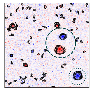
 $\omega /\max {|\omega |}$ for better visualisation of emerging structures. The upper circle highlights a vortex pair and the lower circle marks a single large-scale vortex. Physical quantities for both of these regions are further analysed in figure 4. (c) Kinetic energy spectrum
 $E(k)$ with inset showing the compensated spectrum
 $E(k) k^{5/3} \epsilon _I^{-2/3}$, where the black dashed line indicates a value of
 $C_E = 6.69$ predicted by the test-field model (TFM) closure of Kraichnan (Reference Kraichnan1971). (d) Normalised cross-scale kinetic energy flux
 $Z^E(k)/\epsilon _I$, where the inset shows the normalised enstrophy flux
 $Z^{\varOmega }(k)/\eta _I$.

A discussion of the chosen values of the energy injection rate  $\epsilon _I$ and the general system parameters for the present numerical setup can be found in Appendix B, which is related to the characteristics of structure formation, the kinetic energy spectrum and the cross-scale kinetic energy flux. There, we conclude that run 1 (table 2 in Appendix B) is the best choice for the purpose of our present study. The spatial vorticity distribution in figure 2(b) exhibits a clearly developed population of visually distinguishable vortices or coherent structures. The kinetic energy spectrum in figure 2(c) deviates from the theoretically expected
 $k^{-5/3}$ scaling due to finite-size effects discussed in Appendix B, but we deem it to be more adequate for the subsequent analysis due to a more clearly discernible structuring of the flow. The cross-scale kinetic energy and enstrophy fluxes shown in figure 2(d) possess sufficiently extended ranges of inverse and direct spectral transfer. This facilitates the cross-scale flux decompositions in §§ 6.1 and 6.2.
5.1. Structure detection
As already mentioned in the previous §§ 3.2 and 3.3, the threshold choice for the VM, the f-FTLE and the b-FTLE criterion to sample coherent regions from the vorticity distribution is not straightforward. Therefore, the threshold is chosen such that the three-subregime structure of the coherent vortex number density,  $n(A)$, in (3.3) is realised most clearly. The system studied by Burgess & Scott (Reference Burgess and Scott2017, Reference Burgess and Scott2018) assumed stationarity by imposing an integral length scale far below the largest length scales of the system domain. In contrast, our system is in a statistically stationary state with constant kinetic energy
 $E$ and enstrophy
 $\varOmega$ according to figure 2(a). Therefore, we analyse the scaling sensitivity of the number density
 $n(A)$ only in dependence of the coherent area
 $A$ without the time
 $t$, as presented in figure 3(b,e,h,
 $k$).
Coherent structures, number density and kinetic energy spectra obtained by the VM (a–c), OW criterion (d–f), f-FTLE (g–i) and b-FTLE ( j—l), respectively. The coherent areas are colour-coded matching the normalised number densities  $n(A)/N$ and the decomposed energy spectra, with
 $N$ the total number of detected structures. Colour code: (i) lowest area occupation, green regions corresponding to the green lines of the number density and decomposed energy spectra plots; (ii) intermediate area occupation, green+blue regions corresponding to the blue lines; and (iii) largest area occupation, green+blue+red regions corresponding to the red lines. The OW criterion has only one permitted threshold, hence only a single area occupation is shown. All the energy spectra are compensated by
 $k^{-5/3}$, with the black solid line indicating the total energy spectrum
 $E(k)$, and the coloured solid and dashed lines denoting the coherent
 $E_{c}(k)$ and residual
 $E_{r}(k)$ spectra, respectively. The black dotted horizontal line visualises deviations from the
 $k^{-5/3}$ scaling.

Our comparison of coherence specifications and detection methods begins with the VM criterion. This approach is technically closest to the detection method chosen in Burgess & Scott (Reference Burgess and Scott2017, Reference Burgess and Scott2018) and, thus, expected and observed to yield the best agreement with the findings published there and with the corresponding asymptotic scaling laws of the vortex number density,  $n(A)$. We vary the VM threshold introduced in § 3.2 with three different values
 $\epsilon _{thr}=1.1 \omega _{rms}$,
 $0.9 \omega _{rms}$ and
 $0.7 \omega _{rms}$, for which the total areas occupied by the coherent regions in figure 3(a) amount to
 $3.4\,\%$,
 $6.1\,\%$ and
 $13.5\,\%$, respectively. Filamentary structures occur with increasing area occupation extending the thermal bath regime in figure 3(b). The number density approximately exhibits the phenomenologically proposed asymptotic
 $A^{-3}$ scaling for the highest area occupation. The approximate power law deteriorates as the threshold is raised and the detected set comprises of fewer structures. As the VM criterion explicitly detects regions of high vorticity, the most energetic regions of the flow are included in the coherent part, which is evident from the decomposed kinetic energy spectra in figure 3(c). Most of the energy is concentrated in
 $E_c(k)$, whereas the energy in the residual spectrum
 $E_r(k)$ decreases for larger length scales with scalings which become flatter than
 $k^{-5/3}$ for increasing area occupations. The clearly discernible intermediate region exhibits an increased fluctuation level for lower thresholds because larger and, thus, fewer structures tend to be detected. This is consistent with larger deviations of the measured scaling exponent from the predicted value than in the case of the thermal bath as presented in table 1.
Logarithmic power-law scalings of the three-part vortex number densities  $n(A)$ corresponding to structures detected by the VM (
 $\epsilon _{thr}=0.9 \omega _{rms}$, area occupation:
 $6.1\,\%$), OW criterion, f-FTLE (
 $\epsilon _{thr} = 0.905 \varLambda _{t_0,rms}^{t_0+T_{eddy}}$, area occupation:
 $6.0\,\%$) and b-FTLE (
 $\epsilon _{thr} = 0.915 \varLambda _{t_0,rms}^{t_0-T_{eddy}}$, area occupation:
 $6.8\,\%$), respectively. The scaling ranges are denoted as (i) thermal bath
 $A_f \leq A < A_-$, (ii) intermediate
 $A_- < A < A_+$, and (iii) front
 $A_+ < A \leq A_{max}$. Scaling exponents based on linear regression are given together with the respective standard deviation. The transitional areas
 $A_-$ and
 $A_+$ are estimated from figure 3(b,e,h,k). For simplicity, the forcing-scale area
 $A_f$ and the maximum vortex area
 $A_{\max }$ are chosen as the first and last data points of the respective abscissae of
 $n(A)$.

In contrast to the VM method, the OW criterion only permits one possible threshold  $\epsilon _{thr}=0$. The detected coherent regions in figure 3(d) amount to an area occupation of
 $5.3\,\%$. The thermal bath range obtained via the OW method drops steeper with increasing area
 $A$ than for the VM technique (cf. table 1). This indicates a preference of the OW criterion for intense vortices at the cost of lesser vortical structures in the interval
 $A_f \leq A < A_-$. The intermediate range of the number density
 $n(A)$ in figure 3(e) has the best fulfillment of the
 $A^{-1}$ scaling compared with the other methods according to table 1. This is not surprising, because the OW criterion favours circularly shaped structures, which are also detected by the modified vorticity threshold criterion used by Burgess & Scott (Reference Burgess and Scott2017, Reference Burgess and Scott2018). The residual energy spectrum
 $E_r(k)$ in figure 3( f) possesses a scaling closer to
 $k^{-5/3}$ in the inertial range from
 $k \approx 10$–200 versus the total spectrum
 $E(k)$. In comparison, the coherent spectrum
 $E_c(k)$ has a much shorter
 $k^{-5/3}$ scaling range from
 $k \approx 10-30$, which becomes shallower for increasing wavenumbers. This indicates that the lacking energetic self-similarity of largest-scale coherent structures detected by the OW criterion pollutes the scaling of the theoretically expected KLB spectrum of total energy (see Appendix B). The residual energy whose scaling is not suffering from this specific finite-size effect of the numerical simulation exhibits good agreement with KLB expectations, see also, e.g., Borue (Reference Borue1994), Scott (Reference Scott2007), Vallgren (Reference Vallgren2011) and Burgess & Scott (Reference Burgess and Scott2018).
With regard to the sensitivity of the LCS detection, presented in § 3.3, we set the thresholds of the f-FTLE sampling scheme to  $\epsilon _{thr} = 0.87 \varLambda _{t_0,rms}^{t_0+T_{eddy}}$,
 $0.905 \varLambda _{t_0,rms}^{t_0+T_{eddy}}$ and
 $0.94 \varLambda _{t_0,rms}^{t_0+T_{eddy}}$, which amount to coherent area occupations of
 $3.1\,\%$,
 $6.0\,\%$ and
 $11.2\,\%$, respectively. The thresholds for the b-FTLE are set to
 $\epsilon _{thr} = 0.88 \varLambda _{t_0,rms}^{t_0-T_{eddy}}$,
 $0.915 \varLambda _{t_0,rms}^{t_0-T_{eddy}}$ and
 $0.94 \varLambda _{t_0,rms}^{t_0-T_{eddy}}$, resulting in coherent area occupations of
 $3.3\,\%$,
 $6.8\,\%$ and
 $10.9\,\%$, respectively. The crinkly shaped structures occurring in the domain, as shown in figure 3(g,j), lead to the flattening of the thermal bath regime and a simultaneous steepening of the intermediate range with increasing area occupation, as depicted in figure 3(h,k). Note that the different structural shape also results in a more extended thermal bath regime and a diminishing intermediate range with increasing area occupation in contrast to the OW and VM criterion. Comparing f-FTLE and b-FTLE fields, similar larger-sized structures are detected by both fields, whereas smaller-sized structures are detected at differing positions. This is not surprising, because forward- and backward-in-time LCSs, are associated with different fluid dynamics, i.e. repelling and attracting manifolds in a dynamical systems sense, respectively (Haller & Yuan Reference Haller and Yuan2000; Haller Reference Haller2015). The residual energy spectra
 $E_r(k)$ in figure 3(i,l) are closer to a
 $k^{-5/3}$ scaling throughout the entire inertial range compared with the total spectrum
 $E(k)$, indicating a pollution of the KLB spectrum by the coherent structures similar to the results of the OW criterion.
The large-scale damping required for the achieving stationarity impacts the apparition of large-scale structures as discussed in Appendix B. This leads to the anomalous and partially polluted power laws of the front regime in figure 3(b,e,h,k) compared with the phenomenologically expected exponent of  $A^{-6}$ (Burgess & Scott Reference Burgess and Scott2017, Reference Burgess and Scott2018), where a large-scale damping mechanism has not been employed. Another reason for the deviation is the resolution of
 $8192^2$ in the conducted DNS of Burgess & Scott (Reference Burgess and Scott2017, Reference Burgess and Scott2018), which is higher compared with our present study. Nevertheless, the overall trend of the three-part number density
 $n(A)$ is satisfied in all of these definitions. Moreover, independent of the definition, coherent structures tend to distort the theoretically predicted KLB scaling as illustrated in figure 3(c, f,i,l).
In summary and in comparison with the VM detection technique the OW and the LCS approaches tend to detect similar large-scale coherence features of the flow, in spite of their distinct underlying coherence specifications. The different characterisations of coherence lead to a reduced sensitivity for small-scale turbulent structures in the case of OW, while the physically most involved LCS method tends to detect a surplus of small-scale structures compared with the most simple VM specification. We proceed by setting the respective detection parameters such that the detection signatures as shown in figure 3(b,e,h,k) become most similar to each other, i.e. an area occupation of 6.1 % for VM, of 6.0 % for f-FTLE and of 6.8 % for b-FTLE. The resulting scalings in table 1 reflect a rough overall agreement with the three expected scaling regimes of the number density  $n(A)$. Small adjustments of these thresholds do not result into qualitatively significant differences regarding the inverse cascade analysis, which is conducted in the next section.
6. Relation of coherent structures to the inverse cascade process
Coherent features of the vorticity field  $\omega$ (shown in figure 2b) contain most of its kinetic energy, as inferred from the spatial distribution from the absolute velocity
 $| \boldsymbol {u} |$ in figure 4(a), with the largest fraction located in the vicinity of the vortex core. For the vortex pair in figure 2(b), the energy increases towards their separatrix where the maximum value is reached.
Various physical quantities of the same region as shown in figure 2(b). (a) Absolute velocity  $| \boldsymbol {u} |$. (b) Energy rate
 $dE/dt$. (c) The f-FTLE
 $\varLambda _{t_0}^{t_0+T_{eddy}}$. (d) The b-FTLE
 $\varLambda _{t_0}^{t_0-T_{eddy}}$. (e) Cross-scale kinetic energy flux
 $\bar {Z}$ obtained from a smooth Gaussian filter with a filtering wavenumber of
 $k=60$. ( f) Angle between strain rate and subgrid stress tensor
 $\delta \bar {\theta }$ obtained from the same filter as in (e).

The f-FTLE and b-FTLE fields,  $\varLambda _{t_0}^{t_0+T_{eddy}}$ and
 $\varLambda _{t_0}^{t_0-T_{eddy}}$, are illustrated in figures 4(c) and 4(d), respectively, where high FTLE values are potential candidates for LCSs. The LCS method considered here detects coherent vortices by the characteristic patterns of two-particle dispersion dynamics perpendicular to the identified material lines that are shown in the figure. From this perspective, the approach senses the imprint of a coherent structure on the surrounding flow rather than detecting specific differential (OW) or amplitude markers (VM) associated with coherence. LCS can thus be regarded as complementary to the two other methods considered here. The LCS based on the f-FTLE field displays more pronounced small-scale fluctuations perpendicular to the respective material line as compared with the b-FTLE field. This reflects the different repelling and attracting dynamics expected along forward- and backward-in-time LCSs, while the difference between the Lagrangian scheme used for the f-FTLE and the semi-Lagrangian approach employed for the b-FTLE (see Appendix A.2) can play a role here as well. There is a strong visual correlation between ridges in both FTLE fields with the boundaries of vortices observed in the vorticity field. This corroborates the above choice of sampling the vorticity distribution with the f-FTLE and b-FTLE according to (2.4) and (2.5).
6.1. Cross-scale flux efficiency
When aiming at establishing a link between the nonlinear cross-scale flux and the detected structures in configuration space, the temporal derivative of energy,  $\textrm {d}E/\textrm {d}t$, see figure 4(b), is only of limited value as it does not yield clear localised signatures correlated with coherent vortices. In contrast, the spatial distribution of the cross-scale energy flux
 $\bar {Z}$ exhibits intense quadrupolar structures in coherent regions reflecting their high level of symmetry. This is shown in figure 4(e) and has been observed by Xiao et al. (Reference Xiao, Wan, Chen and Eyink2009) and Liao & Ouellette (Reference Liao and Ouellette2013) as well. Thus, coherent regions lead to large local contributions to the cross-scale flux, but do not necessarily generate significant contributions to the spatially averaged net inverse flux
 $\langle \bar {Z} \rangle$.
The cross-scale energy flux is decomposed into its coherent, residual and mixed contributions, for the spectral cross-scale fluxes  $Z_{c,c,c}^E(k)$,
 $Z_{r,r,r}^E(k)$,
 $Z_{cr}^E(k)$ (4.4) and the spatially averaged cross-scale flux distributions in configuration space
 $\langle \bar {Z}_c(\boldsymbol {x}) \rangle$,
 $\langle \bar {Z}_r(\boldsymbol {x}) \rangle$,
 $\langle \bar {Z}_{cr}(\boldsymbol {x}) \rangle$ (4.8), respectively. Both cross-scale flux measurements are shown in figure 5, because the
 $Z^E(k)$ representation is usually favoured for quantifying the existence of turbulent cascade activity, whereas the
 $\bar {Z}(\boldsymbol {x})$ representation is commonly used to reveal the spatial structure of the flux. We observe that the fluxes of all coherence definitions are qualitatively similar, although the OW criterion in figure 5(b), and the f-/b-FTLE in figures 5(c) and 5(d), respectively, possess higher quantitative similarity in contrast to the VM scheme. For the latter, the coherent flux
 $Z_{c,c,c}^E(k)$ is slightly higher for all scales as shown in figure 5(a) which shows the limits of the applied simple gauge criterion. This is because the VM favourably extracts higher-valued vorticity regions compared with the other detection schemes, which are attributed to larger-sized structures according to the coherent spectrum
 $E_c(k)$ in figure 3(c). Therefore, the highest coherent flux contributions are rather in the lower wavenumber range, with a decreasing contribution towards higher wavenumbers. The structures detected by the f-FTLEs and b-FTLEs have vanishing coherent flux contributions, which are close to zero for the entire inertial range. This is in agreement with both forward- and backward-in-time LCSs, having the tendency to collectively inhibit the energy transfer among scales (Kelley et al. Reference Kelley, Allshouse and Ouellette2013). The circularly shaped structures identified by the OW criterion also exhibit the same behaviour of inhibiting the cross-scale flux. These observations contribute to an alternative definition of coherence in a turbulence context in the sense that energy within these structures tends to remain rather closely at their given length scales without cascading across scales.
Comparison of cross-scale kinetic energy fluxes of varying coherence definitions, obtained from the spectral formulation  $Z^E(k)$ (dashed lines) and the spatially averaged formulation
 $\langle \bar {Z}(\boldsymbol {x}) \rangle$ (solid lines) obtained by Gaussian filtering for varying filter length scales
 $\ell$: (a) VM, (b) OW, (c) f-FTLE and (d) b-FTLE. The grey vertical line indicates the wavenumber
 $k=60$, at which the subsequent analysis of the spatial cross-scale flux distribution is conducted.

In general, the merging of coherent vortices has been one of the most appealing physical mechanisms for the inverse cascade for quite some time. However, independent of the definition and as shown above, the coherent part of the flux  $Z_{c,c,c}^E(k)$ has an overall low negative contribution throughout the inertial range. Therefore, merging effects of coherent structures have a weak influence to the overall inverse cascade, which also has been pointed out by Xiao et al. (Reference Xiao, Wan, Chen and Eyink2009).
The residual flux  $Z_{r,r,r}^E(k)$ remains negative throughout the inertial range as well, peaking at small-scales, close to the forcing wavenumbers, and decaying roughly logarithmically towards larger scales. This is due to the contribution of detected smaller-sized structures, according to the residual spectra
 $E_r(k)$ already shown in figure 3(c, f,i,l) above. We propose in § 6.2 that the negative contribution of the residual flux is attributed to a stronger impact of the thinning mechanism on smaller scales.
Furthermore, a substantial amount of the net negative flux on each length scale originates from the mixed coherent–residual interactions  $Z_{cr}^E(k)$, which roughly stays at a constant level throughout the inverse flux region. We abstain from ascribing this flux contribution to more specific physical dynamics as this flux results from the complex interplay between coherent/residual/mixed stresses and coherent/residual strain rates as already mentioned in § 4.2.
Because the Fourier cross-scale flux is determined via spatial integration, an investigation in configuration space is reasonable for gaining further insight. The coherent part  $\bar {Z}_c(\boldsymbol {x})$ reconstructed from
 $\omega _c$ mostly consists of highly ordered quadrupolar structures and is exemplarily illustrated for the VM criterion in figure 6(a). Compared with that, the
 $\omega _r$-reconstructed residual part
 $\bar {Z}_r(\boldsymbol {x})$ in figure 6(b) has rather complex and unordered spatial features. Similar spatial characteristics for coherent and residual parts are obtained for the other coherence-detection methods. In addition, qualitatively similar findings are gained for filtering lengths below the damping-dominated and above the forcing-dominated length scales, hence we employ a filtering wavenumber of
 $k=60$ for the remaining analysis.
Reconstructed spatial cross-scale kinetic energy flux distributions of the (a) purely coherent  $\bar {Z}_c(\boldsymbol {x})$ and (b) purely residual
 $\bar {Z}_r(\boldsymbol {x})$ parts obtained by the VM criterion for a filtering wavenumber of
 $k=60$, with each normalised by its root-mean-square value for visualisation purposes. The absolute values of
 $\bar {Z}_c$ are much higher compared with
 $\bar {Z}_r$ with a ratio
 ${\max (|\bar {Z}_c|)}/{\max (|\bar {Z}_r|)} \approx 44$.

Another observation, in the context of the present work, is that coherent structures, independent of their detection method, have much higher local cross-scale flux amplitudes compared with their residual counterparts. Using the VM criterion as an example, the ratio between the maximum absolute values of the  $\omega _c$-reconstructed and the
 $\omega _r$-reconstructed spatial cross-scale fluxes is
 ${\max (|\bar {Z}_c|)}/{\max (|\bar {Z}_r|)} \approx 44$. Similar ratios are obtained for the other coherence definitions. However, high amplitudes are not necessarily responsible for a high net inverse flux. As a general observation, the probability density function (p.d.f.) of the total cross-scale flux
 $\bar {Z}$, used for reference for the comparison with the various coherence schemes shown in figure 7(a–d), centralises around zero with a slightly negative skewness of
 $\tilde {\mu }_3 = -0.93$. Furthermore, the p.d.f. has a kurtosis of
 $\tilde {\mu }_4 = 336$ corresponding to a very flat distribution, which indicates that rare high negative amplitude events contribute to the total net negative flux. The p.d.f.s of the coherent parts
 $\bar {Z}_c$ of all coherence definitions exhibit larger tails to both positive and negative values compared with the total field, with kurtosis values of
 $404$,
 $430$,
 $503$ and
 $547$ for the VM, OW criterion, f-FTLE, and b-FTLE, respectively. This suggests that coherent structures are responsible for the high spatial fluctuations of the total cross-scale flux distribution, although these strong fluctuations do not sustain a cascade as already seen before with the overall low Fourier cross-scale flux contributions in figure 5(a–d). In contrast, the p.d.f.s of the residual contributions
 $\bar {Z}_r$ possess lower tails to both positive and negative values. The negative skewness values of
 $-0.76$,
 $-1.4$,
 $-2.01$, and
 $-0.96$ for the VM, OW criterion, f-FTLE, and b-FTLE, respectively, lead to a measurable net inverse cascade of the residual part. However, due to the overall flat nature of the residual p.d.f.s, the residual cascade is also driven by rare high negative amplitude events.
All quantities are filtered at a wavenumber of  $k=60$. (a–d) The p.d.f.s of spatial cross-scale flux distributions
 $\bar {Z}$,
 $\bar {Z}_c$ and
 $\bar {Z}_r$ with each normalised by its standard deviation
 $\bar {Z}^{SD}$,
 $\bar {Z}_c^{SD}$ and
 $\bar {Z}_r^{SD}$, respectively. (e–h) The p.d.f.s of rotation angle distributions between strain-rate and subgrid stress tensors
 $\delta \bar {\theta }$,
 $\delta \bar {\theta }_c$ and
 $\delta \bar {\theta }_r$. (a) VM, (b) OW, (c) f-FTLE, (d) b-FTLE, (e) VM, (f ) OW, (g) f-FTLE, (h) b-FTLE.

The angle distributions between stress and strain-rate tensors as a flux transfer efficiency measure, motivated by (4.9) and (4.10), is shown in figure 4( f), where the largest part of the marked coherent regions display angles close to  $\delta \bar {\theta } = {\rm \pi}/4$. The corresponding misalignment of strain-rate and subfilter stress tensors results in a lower nonlinear flux efficiency. A clearer picture of the overall cascade direction tendencies is obtained from the p.d.f.s of
 $\delta \bar {\theta }$,
 $\delta \bar {\theta }_c$ and
 $\delta \bar {\theta }_r$ shown in figure 7(e–h). The p.d.f. of the total field
 $\delta \bar {\theta }$ clearly shifts towards values smaller than
 ${\rm \pi} /4$, with skewness and kurtosis values of
 $\tilde {\mu }_3 = 0.06$ and
 $\tilde {\mu }_4 = 3.79$, respectively. This indicates that the strain-rate and stress tensors,
 $\bar {\boldsymbol{\mathsf{S}}}$ and
 $\bar {\boldsymbol {\tau }}$, tend to positively align, which lead to the overall net negative flux. However, the shape of all the p.d.f.s of the coherent parts
 $\delta \bar {\theta }_c$ are mostly symmetric and centred at a value of
 ${\rm \pi} /4$ with skewness values
 $0.06$,
 $0.02$,
 $0.0$, and
 $0.03$ for the VM, OW criterion, f-FTLE and b-FTLE, respectively. Thus, the coherent strain-rate and stress tensors,
 $\bar {\boldsymbol{\mathsf{S}}}_c$ and
 $\bar {\boldsymbol {\tau }}_{c,c}$, have the tendency to fully misalign, resulting in a lower cross-scale flux efficiency, despite their high local flux amplitudes. On the contrary, the p.d.f.s of the residual parts
 $\delta \bar {\theta }_r$ skew even more to the right compared with the total field
 $\delta \bar {\theta }$, with skewness values of
 $0.14$,
 $0.13$,
 $0.12$, and
 $0.11$ for the VM, OW criterion, f-FTLE and b-FTLE, respectively. In addition, for the OW criterion in figure 7( f), for the f-FTLE in figure 7(g), and for the b-FTLE in figure 7(h), the left tails of the residual parts
 $\delta \bar {\theta }_r$ are even higher and the right tails even lower compared with their corresponding coherent counterparts
 $\delta \bar {\theta }_c$. These tendencies lead to a higher stress-strain tensor alignment behaviour and thus a higher cross-scale flux efficiency of the residual compared with the coherent part.
We conclude that although strong nonlinear cross-scale flux interactions are found within the quadrupolar structures of figure 6(a), these high local flux amplitudes are not responsible for an actual cascade process. They are rather responsible for sustaining the structures’ coherence in a turbulent environment by keeping the associated energy close to specific length scales.
6.2. Coherent shape preservation and residual thinning mechanism
A possible reason for the small coherent Fourier cross-scale flux contributions is the shape preservation of coherent structures in combination with the enhanced flux efficiency of the residual part due to increased vortex thinning. To verify this hypothesis, the MSG expanded cross-scale energy flux in (4.13) and its decomposed form in (4.17) and (4.18) are investigated in more detail with a filtering length of  $\ell ={\rm \pi} /15$, a geometric factor of
 $\lambda =2$ and a total number of filter bands of
 $n_b=5$. For a detailed analysis the flux fractions
 $Q^{[b]}$ on different subfilter-scales are divided into
 \begin{equation} Q^{[b]} = \frac{\langle Z_{SR}^{[b]} \rangle + \langle Z_{DSR}^{[b]} \rangle + \langle Z_{DSM}^{[b]} \rangle + \langle Z_{VGS}^{[b]} \rangle}{\langle Z_{*}^{MSG} \rangle} = Q_{SR}^{[b]} + Q_{DSR}^{[b]} + Q_{DSM}^{[b]} + Q_{VGS}^{[b]}, \end{equation}
where  $Q_{SR}^{[b]}$,
 $Q_{DSR}^{[b]}$,
 $Q_{DSM}^{[b]}$ and
 $Q_{VGS}^{[b]}$ are the flux fractions resulting from SR, DSR, DSM and VGS, respectively. All the flux channels are further decomposed into their coherent (
 $c$), residual (
 $r$) and mixed (
 $cr$) contributions, e.g. the fraction of the SR is decomposed as
 $Q_{SR}^{[b]} = Q_{SR,c}^{[b]} + Q_{SR,r}^{[b]} + Q_{SR,cr}^{[b]}$. All these contributions are illustrated in figure 8.
Second-order MSG flux fractions for the length scale bands in the range of  $b \in [0,5]$ originating from SR
 $Q_{SR}^{[b]}$ (green), DSR
 $Q_{DSR}^{[b]}$ (violet), DSM
 $Q_{DSM}^{[b]}$ (blue), and VGS
 $Q_{VGS}^{[b]}$ (orange) contributions, decoded into their corresponding coherent (subscript
 $c$), residual (subscript
 $r$), and mixed (subscript
 $cr$) parts. The varying coherence criterions are compared for every
 $b$ in the following order: VM, OW criterion, f-FTLE and b-FTLE.

As already discussed by Xiao et al. (Reference Xiao, Wan, Chen and Eyink2009), the MSG flux  $Z_{*}^{MSG}$ exhibits the locality behaviour predicted by the test-field model (TFM) closure of Kraichnan (Reference Kraichnan1971). Thus, it is not surprising in figure 8 that the majority of the contributions do not result from strongly local interactions
 $b=0$, but rather from non-local interactions
 $b \in [1,3]$, with a decreasing influence from highly non-local interactions
 $b \geq 4$, with
 $b$ being a measure of the scale locality of nonlinear interactions. The first-order MSG flux only consists of the SR term
 $Z_{SR}^{[b]}$, which has no contribution to the strongly local interactions (
 $Q_{SR}^{[0]}=0$) (Eyink Reference Eyink2006b; Xiao et al. Reference Xiao, Wan, Chen and Eyink2009). Thus, second-order contributions are necessary to sufficiently capture the cross-scale flux. The DSM
 $Z_{DSM}^{[b]}$ has the lowest overall contribution and is also non-existent for strongly local interactions (
 $Q_{DSM}^{[0]}=0$) (Eyink Reference Eyink2006b; Xiao et al. Reference Xiao, Wan, Chen and Eyink2009). Hence, its effect originating from coherent and residual parts are not further analysed with respect to strain-rate alignment properties.
In figure 8 the relative contributions of the coherent, residual and mixed parts to each flux channel are nearly independent of the scale locality  $b$ and the specific coherence definition. The simple VM method represents a notable exception generally yielding increased coherent flux contributions at the cost of the residual fluxes. As already mentioned above, this is the consequence of the simple gauge criterion chosen in § 5.1 that is not capable of eliminating all differences between the detection methods. Test simulations (not shown) indicate that the VM method is more robust than the LCS techniques to variations of the threshold value with regard to the scaling of the vortex number density, but exhibits a stronger and monotonic impact of the threshold on the relative importance of the different MSG flux fractions than the LCS methods. The gauging procedure thus leads to an effective relative threshold decrease for the VM method compared with the other more complex coherence specifications, illustrating the difficulty of neutralising all differences between the coherence specifications. The flux fractions mostly reflect the decomposed Fourier cross-scale flux contributions already presented in figure 5 above. For example, the f-FTLE criterion has small coherent cross-scale flux contributions
 $Z_{c,c,c}^E(k)$ throughout the inertial range in figure 5(c), and the coherent fractions
 $Q_{SR,c}^{[b]}$,
 $Q_{DSR,c}^{[b]}$,
 $Q_{DSM,c}^{[b]}$, and
 $Q_{VGS,c}^{[b]}$ of the MSG flux in figure 8 are small for all of the flux channels as well, except for the VM method as mentioned above. We associate the lack of substantial SR and VGS of the coherent structures with their shape preservation characteristic. In contrast, the residual fractions
 $Q_{SR,r}^{[b]}$,
 $Q_{DSR,r}^{[b]}$,
 $Q_{DSM,r}^{[b]}$, and
 $Q_{VGS,r}^{[b]}$ have a much higher contribution in all these MSG flux channels, which is also reflected by the residual cross-scale flux
 $Z_{r,r,r}^E(k)$. In addition, the coherent cross-scale flux of the VM criterion is decreasing, while the residual flux is increasing for higher wavenumbers in the inertial range in figure 5(a). This is also reflected by the MSG flux fractions in figure 8. There, the coherent fractions of all MSG flux channels decrease, while the residual fractions increase for lower scale locality. These observations are a first sign that vortex thinning plays a minor role in coherent structures and is more active in the residual counterpart instead. Lastly, similar to the decomposed cross-scale fluxes in figure 5(a–d), the mixed interactions
 $Q_{SR,cr}^{[b]}$,
 $Q_{DSR,cr}^{[b]}$,
 $Q_{DSM,cr}^{[b]}$, and
 $Q_{VGS,cr}^{[b]}$ contribute to almost half of the fractions in all MSG flux channels in figure 8. However, this does not imply that coherent–residual interactions lead to an enhanced thinning mechanism, since the MSG cross-scale flux of the mixed contribution
 $Z_{*,cr}^{MSG}$ in (4.17) consists of four different heterogeneous strain-rate and stress components. We leave the analysis of these heterogeneous interactions for future investigations.
According to the numerical studies of Xiao et al. (Reference Xiao, Wan, Chen and Eyink2009) and as described in § 4.3, the vortex thinning mechanism is geometrically quantified by the rotation angles  $\delta \alpha ^{[b]}$ and
 $\delta \beta ^{[b]}$, which are illustrated in figures 1(b) and 1(c), respectively. Conditioning the angle
 $\delta \alpha ^{[b]}$ onto the band-pass filtered vorticities
 $\omega ^{[b]}$ allows us to obtain statistics of the rotation angle behaviour between the large scale strain-rate
 $\boldsymbol{\mathsf{S}}^{(0)}$ and the band-pass filtered strain-rates
 $\boldsymbol{\mathsf{S}}^{[b]}$, and thus reveals the physical mechanism of the MSG flux contribution originated from the SR term
 $Z_{SR}^{[b]}$ in (4.13). A conditioning of the angle
 $\delta \alpha ^{[b]}$ onto the band-pass filtered eddy-viscosities
 $\nu _T^{[b]}$ allows the analysis of the alignment behaviour between the large scale strain-rate
 $\boldsymbol{\mathsf{S}}^{(0)}$ and the band-pass filtered stress
 $\boldsymbol {\tau }^{[b]} = -\nu _T^{[b]} \boldsymbol{\mathsf{S}}^{[b]}$, which comes from a Newtonian stress-strain relation as already described in § 4.3. From this we are able to infer the physical mechanism of the DSR term
 $Z_{DSR}^{[b]}$ in (4.13), which quantifies the direction of the stress work exertion on the strain-rate field from small to large length scales. Finally, analysing the
 $\delta \beta ^{[b]}$ angle reveals the influence of the VGS mechanism described by
 $Z_{VGS}^{[b]}$ in (4.13). We extend the angle analysis by investigating the angles
 $\delta \alpha _{c/r}^{[b]}$ and
 $\delta \beta _{c/r}^{[b]}$ of the purely coherent and residual contributions based on the (4.19)–(4.24). According to figure 9(b,d, f) all coherence definitions provide similar results regarding the above mentioned angle statistics. Thus, the following observations and conclusions are made for coherent structures in general, independent of the concrete definition.
(a) The p.d.f.s of strain-rate tensor angles  $\delta \alpha ^{[b]}$ conditioned onto the negative vorticities
 $\omega ^{[b]}$. (b) Expected values of
 $\delta \alpha ^{[b]}$,
 $\delta \alpha ^{[b]}_c$ and
 $\delta \alpha ^{[b]}_r$ conditioned onto the negative vorticities
 $\omega ^{[b]}$,
 $\omega ^{[b]}_c$ and
 $\omega ^{[b]}_r$, respectively, for varying coherence definitions. (c) The p.d.f.s of strain-rate tensor angles
 $\delta \alpha ^{[b]}$ conditioned onto the positive eddy-viscosities
 $\nu _T^{[b]}$. (d) Expected values of
 $|\delta \alpha ^{[b]} |$,
 $|\delta \alpha ^{[b]}_c |$ and
 $|\delta \alpha ^{[b]}_r |$ conditioned onto the positive eddy-viscosities
 $\nu _T^{[b]}$,
 $\nu _{T,c}^{[b]}$ and
 $\nu _{T,r}^{[b]}$, respectively, for varying coherence definitions. (e) The p.d.f.s of angles between the large-scale strain-rate tensor and vorticity gradient vector
 $\delta \beta ^{[b]}$. ( f) Expected values of
 $\delta \beta ^{[b]}$,
 $\delta \beta ^{[b]}_c$ and
 $\delta \beta ^{[b]}_r$ for varying coherence definitions.

The closer the angles between the strain-rate tensors  $\delta \alpha ^{[b]}$ are to values of
 $\pm {\rm \pi}/4$ (their sign reflecting the sign of
 $\omega ^{[b]}$), the higher the contribution of the SR term
 $Z_{SR}^{[b]}$ to the inverse cascade. This rotation angle tendency is exemplarily illustrated in figure 9(a) for the negative vorticity condition
 $-\omega ^{[b]}$, for which the peak of the p.d.f.
 $P(\delta \alpha ^{[b]} | \omega ^{[b]} < 0)$ gradually shifts towards
 $+{\rm \pi} /4$ with decreasing scale locality, implied by the increasing
 $b$-values (cf. Xiao et al. Reference Xiao, Wan, Chen and Eyink2009). This gradual peak shift quantifies SR and the accompanied transformation of circularly shaped structures into shear layers. Thus, investigating the presence of SR is one possibility to show the existence of the thinning process for the total field. Therefore, if we measure the shift of the p.d.f. peak, we are able to determine the SR effect separately for the purely coherent and residual parts. We achieve this by evaluating the conditional expectation values of the angles
 $\delta \alpha ^{[b]}$,
 $\delta \alpha ^{[b]}_c$ and
 $\delta \alpha ^{[b]}_r$ as
 \begin{equation} \mathbb{E} [\delta
\alpha^{[b]} | (\omega^{[b]} < 0) ], \mathbb{E}
[\delta \alpha^{[b]}_c | (\omega^{[b]}_c < 0) ],
\mathbb{E} [\delta \alpha^{[b]}_r | (\omega^{[b]}_r <
0) ]. \end{equation}
Figure 9(b) shows that the conditional expectation values for the coherent structures, independent of the concrete definition, are approximately  $\mathbb {E} [\delta \alpha ^{[b]}_c | (\omega ^{[b]}_c < 0) ] \approx 0$. This means that there is only a minor gradual shift of the p.d.f. peak for coherent structures with decreasing scale locality (increasing
 $b$-values). This leads to the conclusion that SR and therefore thinning effects are barely present within structures of the coherent part. Hence, coherent structures are generally not turned into shear layers and tend to preserve their shape. On the contrary, the residual part exhibits an increased expected value
 $\mathbb {E} [\delta \alpha ^{[b]}_r | (\omega ^{[b]}_r < 0) ]$ with decreasing scale locality. Therefore, the background residual field is prone to the development of shear layers and thus has a higher thinning tendency compared with the coherent structures in the system.
The DSR term  $Z_{DSR}^{[b]}$ has an increasing contribution to the overall inverse cascade, if the angle is
 $| \delta \alpha ^{[b]} | \gtrless {\rm \pi}/4$ for positive or negative eddy-viscosities
 $\pm \nu _T^{[b]}$, respectively. Therefore, the band-pass filtered stress tensors
 $\boldsymbol {\tau }^{[b]}$ should exhibit parallel or anti-parallel alignments to the large-scale strain-rate tensor
 $\boldsymbol{\mathsf{S}}^{(0)}$ based on the eddy-viscosity's sign in order to maximise the
 $Z_{DSR}^{[b]}$ contribution. The alignment tendency reveals the energy transfer between scales during the vortex thinning procedure. Thus, negative work exertion of the small-scale stress
 $\boldsymbol {\tau }^{[b]}$ on the large-scale strain-rate field
 $\boldsymbol{\mathsf{S}}^{(0)}$ is understood as a general energy transfer from small to large length scales enabling an overall inverse energy cascade, whereas positive work exertion allows for a direct energy cascade. The p.d.f. of the angles exemplarily conditioned onto the positive eddy-viscosity
 $P(\delta \alpha ^{[b]}|\nu _T^{[b]} > 0)$ for the total field is presented in figure 9(c) and shows that the angle becomes
 $| \delta \alpha ^{[b]} | > {\rm \pi}/4$ for
 $b \geq 3$ (cf. Xiao et al. Reference Xiao, Wan, Chen and Eyink2009). This reveals the negative work exertion of the small-scale stress
 $\boldsymbol {\tau }^{[b]}$ on the large-scale strain-rate tensor
 $\boldsymbol{\mathsf{S}}^{(0)}$, as depicted in figure 1(b), and leads to the conclusion that the vortex thinning mechanism facilitates the energy transfer from small to large length scales for the entire field. The conditional expectation values of the angles
 $\delta \alpha ^{[b]}$,
 $\delta \alpha ^{[b]}_c$ and
 $\delta \alpha ^{[b]}_r$,
 \begin{equation}
\mathbb{E} [| \delta \alpha^{[b]} | | (\nu_T^{[b]} > 0) ],
\mathbb{E} [| \delta \alpha^{[b]}_c| | (\nu_{T,c}^{[b]} > 0)], \mathbb{E}
[| \delta \alpha^{[b]}_r | | (\nu_{T,r}^{[b]} > 0)], \end{equation}
are determined to measure the shift of the maxima towards  $| \delta \alpha ^{[b]} | > {\rm \pi}/4$ for increasing
 $b$-values in figure 9(d) and are also used to determine the alignment tendencies of coherent and residual parts. The absolute values
 $| \delta \alpha ^{[b]} |$ instead of the original angle
 $\delta \alpha ^{[b]}$ are considered, because the p.d.f.s in figure 9(c) are symmetric. As a result, figure 9(d) shows that the negative work exertion is present within the residual parts for
 $b \geq 3$ as the angles become
 $| \delta \alpha ^{[b]}_r | > {\rm \pi}/4$. Although
 $\mathbb {E} [| \delta \alpha ^{[b]}_c | | (\nu _{T,c}^{[b]} > 0) ]$ increases for larger
 $b$, the angles for the coherent structures remain at
 $| \delta \alpha ^{[b]}_c | < {\rm \pi}/4$ independent of the scale locality. This means that the coherent part even has the tendency that the coherent band-pass filtered stress tensors
 $\boldsymbol {\tau }_c^{[b]}$ exert positive instead of negative work on the coherent large-scale strain-rate tensor
 $\boldsymbol{\mathsf{S}}_c^{(0)}$. Thus, energy within coherent structures is not transferred from the small-scale stress to the large-scale strain-rate due to the weak contributions of the thinning mechanism.
Lastly, the VGS term  $Z_{VGS}^{[b]}$ is dependent on the angles
 $\delta \beta ^{[b]}$ between the contractile direction of the large-scale strain-rate
 $\boldsymbol{\mathsf{S}}^{(0)}$ and the vorticity gradients
 $\boldsymbol {\nabla } \omega ^{[b]}$. These angles approach zero
 $\delta \beta ^{[b]} \rightarrow 0$ for decreasing scale locality (increasing
 $b$), as presented in figure 9(e) (cf. Xiao et al. Reference Xiao, Wan, Chen and Eyink2009), which shows the contribution
 $Z_{VGS}^{[b]}$ for the total field. This quantifies the presence of the vorticity isoline deformation along the stretching direction of the large-scale strain-rate field, as depicted in figure 1(b) for the total field. The alignment angles
 $\delta \beta _{c/r}^{[b]}$ between the purely coherent/residual vorticity gradients
 $\boldsymbol {\nabla } \omega _{c/r}^{[b]}$ and the purely coherent/residual contractile direction of the strain-rate tensor
 $\boldsymbol{\mathsf{S}}_{c/r}^{(0)}$ are used to measure the effect of VGS in the coherent and residual parts of the flow respectively. The following expected values
 \begin{equation}
\mathbb{E} [\delta \beta^{[b]}], \mathbb{E} [\delta \beta^{[b]}_c], \mathbb{E} [\delta \beta^{[b]}_r],
\end{equation}
for the total, coherent and residual fields are illustrated in figure 9( f). The expected value for the residual angle  $\mathbb {E} [\delta \beta ^{[b]}_r ]$ decreases for large scale separations (increasing
 $b$), indicating the presence of the VGS in the residual part and thus is another indicator of the thinning mechanism. For the coherent part
 $\mathbb {E} [\delta \beta ^{[b]}_c ]$ is close to
 ${\rm \pi} /4$ for all values of
 $b$. This implies the physical picture that the coherent large-scale strain-rate tensor
 $\boldsymbol{\mathsf{S}}_{c}^{(0)}$ is not distorting the vorticity isolines, which ultimately leads to a shape preservation of coherent structures.
In conclusion, the small cascade efficiency of coherent structures is caused by their shape preserving nature determined by the depletion of  $Z_{SR,c}^{[b]}$ and
 $Z_{VGS,c}^{[b]}$ terms independent of the scale separations
 $b$ in combination with the positive work exertion of the small-scale stresses on the large scale strain-rate, as captured by the
 $Z_{DSR,c}^{[b]}$ term. In contrast, the higher flux efficiency in the residual parts of the flow is caused by the enhanced thinning mechanism quantified by the
 $Z_{SR,r}^{[b]}$ and
 $Z_{VGS,r}^{[b]}$ contributions and the negative work exertion captured in the
 $Z_{DSR,r}^{[b]}$ term.
7. Conclusions
The present investigation deals with the nonlinear dynamics of coherent and residual structures in pseudospectral DNS of two-dimensional Navier–Stokes turbulence forced at small scales. This involves the application of three commonly applied coherence detection schemes based on the OW criterion, on the VM, and on LCSs to identify and to isolate the respective flow components. Among these threshold-based detection methods, the VM technique and the LCS approach are gauged by using statistical properties of detected structures to improve comparability of the detection results. Using this setup, (i) the performance of the employed detection methods is discussed in relation to each other, (ii) the coherent and residual contributions to the cross-scale energy flux of the inverse turbulent cascade have been analysed in spectral Fourier as well as in configuration space to study their role for the characteristics and for the dynamics of the respective parts of the flow.
We have found that (i) under application of the chosen gauge criterion and in comparison with the VM scheme the OW method exhibits a bias towards largest-scale and most energetic structures. In contrast, the LCS scheme shows an increased susceptibility for small-scale coherence as compared with the VM method. Both tendencies can largely be neutralised by adjusting the free parameters of the VM and the LCS methods to yield the same scale-dependency of the vortex number density as the OW specification.
With respect to the role of detected coherent structures for turbulence dynamics, (ii), we find that they are responsible for a pollution of the phenomenologically expected spectral scaling of the kinetic energy spectrum  $E(k)\sim k^{-5/3}$ at largest spatial scales. This finding is supported by the largely unaffected
 $k^{-5/3}$-scaling observed in the energy spectrum of the residual (incoherent) fraction of the turbulent fluctuations. The observation suggests the possible use of coherence detection and decomposition in DNS of homogeneous turbulence for the reduction of the large-scale condensation of inversely cascading quantities for physical systems that feature inverse cascades, e.g. two-dimensional Navier–Stokes turbulence or magnetohydrodynamic turbulence.
The application of a spatial scale-filter approach for the analysis of the nonlinear dynamics of coherent and residual parts of the turbulent flow indicates a high nonlinear activity within coherent structures. The finding shows that coherent structures in two-dimensional Navier–Stokes turbulence are in general dynamically sustained while the spatial structure of the dynamics yields a shape-preserving depletion of the nonlinear cross-scale flux with regard to the entire structure. This is in agreement with the observed coherent Fourier cross-scale energy fluxes and the low flux efficiency due to the high misalignment tendencies of coherent strain-rate and subgrid stress tensors. The shape preservation of coherent structures in this case is verified by employing the MSG expansion of the coherent spatial cross-scale energy fluxes that exhibits a clear depletion of the deformation processes that are scale-flux generating. These findings suggest to employ the depletion of the MSG contributions of SR and VGS as markers for structural coherence in two-dimensional turbulent flows.
The inverse cascade is instead driven by a combination of (i) interactions entirely among residual fluctuations and of (ii) nonlinear interactions between coherent structures and residual fluctuations. The former contribution is strongest at small scales while the latter dominates at large scales. This suggests that two different physical processes are responsible for the respective energy fluxes. For the first contribution the dominant physical process has recently been introduced as vortex thinning. This is in line with the enhanced alignment properties of the residual strain-rate and subgrid stress tensors, yielding a high flux efficiency. The second contribution is the dominant flux contribution and stays on a relatively high and roughly constant level throughout the inverse flux region. We abstain from ascribing this flux contribution to more specific physical dynamics as multiple factors may be determining its characteristics due to the heterogeneous character of the interacting strain-rate and stress tensor fields. Further work is presently being pursued along these directions.
Acknowledgements
The authors thank B. Beck, R. Mäusle, J. Reiss and J.-M. Teissier for fruitful discussions.
Funding
This work was supported by the German Research Foundation (DFG) within the Research Training Group GRK 2433. Computing resources from the Max Planck Computing and Data Facility (MPCDF) are also acknowledged.
Declaration of interests
The authors report no conflict of interest.
Appendix A. Technical details
A.1. Vorticity decomposition
After thresholding according to one of the investigated coherence criteria in the fashion of (2.4) and (2.5), the non-zero scalar values of the vorticity field are clustered. All adjacent neighbouring non-zero pixels (maximum of four neighbours for each pixel) are grouped into separately countable and connected clusters. Then, clusters whose number of pixels are below the forcing area of  $A_f = {\rm \pi}(\ell _f/2)^2$, with
 $\ell _f = 2 {\rm \pi}/k_f$ the forcing length scale, are excluded and discarded from the coherent field. After that, a
 $5 \times 5$ smooth Gaussian filter is applied to avoid regularity issues caused by sharp boundaries. This leads to the coherent vorticity field
 $\omega _c^{smooth}$. The residual field is obtained by subtraction:
 \begin{equation} \omega_r = \omega - \omega_c^{smooth}. \end{equation}
A.2. Efficient FTLE calculation
From a technical viewpoint, integrating larger amounts of Lagrangian tracers to sufficiently resolve a turbulent flow in space and time requires substantial computational resources. Thus, we utilise an efficient numerical technique, as suggested by Finn & Apte (Reference Finn and Apte2013), to simultaneously calculate the flowmap  $\boldsymbol {F}_{t_0}^{t}$ forward and backward in time by employing a Lagrangian and a semi-Lagrangian scheme, respectively. The forward-in-time/Lagrangian scheme advects passive tracers for an integration time
 $T$ according to the underlying velocity field, which generate the forward-in-time flowmap,
 $\boldsymbol {F}_{t_0}^{t_0+T}$. The backward-in-time/semi-Lagrangian scheme, introduced by Leung (Reference Leung2011), is based on the solution of level-set equations and constructs the backward-in-time flowmap,
 $\boldsymbol {F}_{t_0}^{t_0-T}$, by tracking coordinates on an Eulerian grid.
For an increased temporal resolution of the FTLE fields, a flowmap composition method, proposed by Brunton & Rowley (Reference Brunton and Rowley2010), is applied as
 \begin{equation} \boldsymbol{F}_{t_0}^{t_0+T} = \mathcal{I} \boldsymbol{F}_{t_0+(N-1)h}^{t_0+Nh} \circ \ldots \circ \mathcal{I} \boldsymbol{F}_{t_0+h}^{t_0+2h} \circ \boldsymbol{F}_{t_0}^{t_0+h}, \end{equation}
where  $\circ$ is the composition operator,
 $N$ the number of substeps,
 $h=100$ the flowmap substep and
 $\mathcal {I}$ the interpolation operator. A second-order Runge–Kutta integration scheme is applied for particle integration and a cubic interpolation scheme, suggested by Staniforth & Côté (Reference Staniforth and Côté1991), is used for the interpolation operator and the mapping of particles between grid points.
A.3. MSG flux derivation
The multi-gradient nature of the approach arises from a Taylor expansion
 \begin{equation} \delta \boldsymbol{u}^{(b,m)}(\boldsymbol{r};\boldsymbol{x}) = \sum_{p=1}^{m} \frac{1}{p!} (\boldsymbol{r} \boldsymbol{\cdot} \boldsymbol{\nabla})^p \boldsymbol{u}^{({b})}(\boldsymbol{x}) \end{equation}
of the filtered velocity increments  $\delta \boldsymbol {u}^{({b})}(\boldsymbol {r};\boldsymbol {x}) = \boldsymbol {u}^{({b})}(\boldsymbol {x}+\boldsymbol {r}) - \boldsymbol {u}^{({b})}(\boldsymbol {x})$ with separation vector
 $\boldsymbol {r}$, which is subject to the filtering operation given by equation (4.11). The filtered subgrid stress tensor
 $\boldsymbol {\tau }^{({b})}$ can then be entirely expressed by the Taylor expanded velocity increments instead of the original increments
 $\delta \boldsymbol {u}^{({b})}(\boldsymbol {r})$. This yields (cf. Eyink Reference Eyink2006a)
 \begin{align} \boldsymbol{\tau}^{(b,m)} &= \int G_l(\boldsymbol{r}) \delta \boldsymbol{u}^{(b,m)}(\boldsymbol{r}) \delta \boldsymbol{u}^{(b,m)}(\boldsymbol{r}) \,\mathrm{d}^2 \boldsymbol{r} \nonumber\\ &\quad - \int G_l(\boldsymbol{r}) \delta \boldsymbol{u}^{(b,m)}(\boldsymbol{r}) \,\mathrm{d}^2 \boldsymbol{r} \int G_l(\boldsymbol{r}) \delta \boldsymbol{u}^{(b,m)}(\boldsymbol{r}) \,\mathrm{d}^2 \boldsymbol{r}, \end{align}
where  $\boldsymbol {\tau }^{(b,m)}$ is a multi-scale and multi-gradient expression for the stress.
It can be shown that the MSG expanded stress converges as  $\lim _{m \rightarrow \infty } \boldsymbol {\tau }^{(b,m)} = \boldsymbol {\tau }^{({b})}$ in the
 $L^1$-norm. Nevertheless, for increasing scale indices
 $b$, which corresponds to adding finer-scale structures, a growing amount of space gradients of higher-order,
 $m$, is required to approximate
 $\boldsymbol {\tau }^{(b,m)} \approx \boldsymbol {\tau }^{({b})}$. Therefore, a coherent-subregions approximation (CSA) approach is suggested by Eyink (Reference Eyink2006a) enabling the approximation of the MSG stress by low-order gradients
 $m$. As a result, the CSA corrected MSG stress is obtained, which is more accurately approximated as
 $\boldsymbol {\tau }^{(b,m)}_{*} \approx \boldsymbol {\tau }^{(b,m)}$ with fewer gradients
 $m$. According to Eyink (Reference Eyink2006b) and Xiao et al. (Reference Xiao, Wan, Chen and Eyink2009), the best approximation with regard to the original cross-scale flux term is reached for expansions up to the second-order in gradients
 $m=2$. For the sake of brevity we define
 $\boldsymbol {\tau }_{*}^{MSG}=\boldsymbol {\tau }_{*}^{(b,2)}$ and
 $Z_{*}^{MSG} = Z_{*}^{(b,2)}$, which are the MSG-CSA stress and cross-scale flux, respectively, expanded to second order, giving
 \begin{align} Z_{*}^{MSG} &={-} \boldsymbol{\mathsf{S}}^{(0)} : \boldsymbol{\tau}_{*}^{MSG} \nonumber\\ &= \sum_{b=0}^{n_b} \left[ \underbrace{-\frac{\bar{C}_2^{[b]}}{2} \ell_b^2 \omega^{[b]} (\boldsymbol{\mathsf{S}}^{(0)} : \tilde{\boldsymbol{\mathsf{S}}}^{[b]})}_{Z_{SR}^{[b]}} \underbrace{ + \frac{\bar{C}_4^{[b]}}{8} \ell_b^4 (\overbrace{\boldsymbol{\nabla} \omega^{[b]} \boldsymbol{\cdot} \boldsymbol{\nabla} \alpha^{[b]}}^{\nu_T^{[b]}}) (\boldsymbol{\mathsf{S}}^{(0)} : \boldsymbol{\mathsf{S}}^{[b]})}_{Z_{DSR}^{[b]}} \right.\nonumber\\ &\quad\left.\underbrace{-\frac{\bar{C}_4^{[b]}}{16} \ell_b^4 (\overbrace{\boldsymbol{\nabla} \omega^{[b]} \boldsymbol{\cdot} \boldsymbol{\nabla} \ln \sigma^{[b]}}^{\gamma_T^{[b]}}) (\boldsymbol{\mathsf{S}}^{(0)} : \tilde{\boldsymbol{\mathsf{S}}}^{[b]})}_{Z_{DSM}^{[b]}} \underbrace{+ \frac{\bar{C}_4^{[b]}}{32} \ell_b^4 (\boldsymbol{\nabla} \omega^{[b]})^{{\rm T}} \boldsymbol{\mathsf{S}}^{(0)} (\boldsymbol{\nabla} \omega^{[b]})}_{Z_{VGS}^{[b]}} \right] \nonumber\\ & \quad\underbrace{- (\boldsymbol{\nabla} \psi_{*}^{(n_b)})^{{\rm T}} \boldsymbol{\mathsf{S}}^{(0)} (\boldsymbol{\nabla} \psi_{*}^{(n_b)})}_{Z_{FSF}^{(n_b)}}, \end{align}
with the fluctuation stream function  $\psi _{*}^{(n_b)}$ (cf. Eyink Reference Eyink2006b) and the coefficients
 $\bar {C}_p^{[b]}$ (cf. appendix C in Eyink Reference Eyink2006a). The flux contribution from the fluctuation stream function (FSF)
 $Z_{FSF}^{(n_b)}$ is similarly interpreted as a VGS but considered much smaller in magnitude due to cancellations from spatial averaging. In addition, it possesses a positive mean as shown by Xiao et al. (Reference Xiao, Wan, Chen and Eyink2009), thus a further analysis with regard to the inverse cascade mechanism is neglected for this term.
Appendix B. Sensitivity of energy injection rate, KLB theory and finite-size effects
The present coherent structure analysis is based on DNS of the two-dimensional Navier–Stokes equations. In this section, we briefly discuss the choice of system parameters, with regard to the dynamics of structure formation and turbulence statistics.
In contrast to other studies (see Babiano et al. Reference Babiano, Basdevant, Legras and Sadourny1987; Maltrud & Vallis Reference Maltrud and Vallis1993; Borue Reference Borue1994; Danilov & Gurarie Reference Danilov and Gurarie2001; Vallgren Reference Vallgren2011; Burgess & Scott Reference Burgess and Scott2018), the present work does not employ a hyperviscous dissipation term to avoid the accompanying unphysical distortion of the spatial structure of the flow. Although this shortens the scaling-range of the enstrophy cascade, the resulting spectral extent still suffices for our purposes, as shown by the spectra and enstrophy fluxes in figure 2(c,d), and figure 10. We have found no further implications for other diagnostics relevant in the context of the present investigation.
Kinetic energy spectra  $E(k)$ of runs 2 and 3 with varying kinetic energy injection rates (a) with inset showing the compensated spectra
 $E(k) k^{5/3} \epsilon _I^{-2/3}$, where the black dashed line indicates a value of
 $C_E = 6.69$ predicted by the TFM closure of Kraichnan (Reference Kraichnan1971). Normalised cross-scale kinetic energy
 $Z^E(k)/\epsilon _I$ (b) and enstrophy fluxes
 $Z^{\varOmega }(k)/\eta _I$ (c) from runs 2 and 3, respectively.

The formation of structures is dependent on the energy injection rate  $\epsilon _I$ and therefore we vary its rate for fixed viscosity
 $\nu$ and large-scale friction values (
 $k_{0,\omega }$,
 $\sigma _{\omega }^2$,
 $\alpha _{\omega }$), which also affects the ratio of energy dissipated at largest scales with rate
 $\epsilon _{\alpha }$ and at viscous scales with rate
 $\epsilon _{\nu }$. Due to the unavoidably limited spectral bandwidth of the numerical simulations, it is not possible to fulfil both requirements of the KLB picture at the same time, namely a ratio of
 $\epsilon _{\alpha }/\epsilon _I = 1$, such that all the injected energy is dissipated at large-scales, in combination with an exact power-law
 $\sim k^{-5/3}$ for the energy scaling-range. Even DNS at significantly higher numerical resolution (see e.g. Boffetta & Musacchio Reference Boffetta and Musacchio2010) exhibit smaller deviations from the asymptotic scaling exponent. We observe, that simultaneously only one of the two characteristics is approximately realisable with sufficient accuracy. Therefore, three simulation runs are performed, as listed in table 2. Next to numerical resolution and the large-scale damping required for quasi-stationarity of the flow, the large-scale driving, i.e. the energy injection rate
 $\epsilon _I$, exerts an important influence on the system.
Simulation parameters of the two-dimensional hydrodynamic turbulence system with a resolution of  $4096^2$, forcing wavenumber
 $k_f = 200$, large-scale friction factor
 $\alpha _{\omega }=500$, centre of Gaussian damping profile
 $k_{0,\omega } = 0.1$, variance of the Gaussian
 $\sigma _{\omega }^2 = 1$, viscosity
 $\nu =5 \times 10^{-5}$ and timestep
 $\textrm {d}t=5 \times 10^{-6}$.

According to figure 2(c), run 1 with the highest energy injection rate exhibits the strongest deviation from the  $k^{-5/3}$ scaling, but the best developed normalised cross-scale energy
 $Z^E(k)/\epsilon _I$ and enstrophy fluxes
 $Z^{\varOmega }(k)/\eta _I$ (figure 2d) close to values of
 $-1$ and
 $1$ in the energy and enstrophy inertial ranges, respectively. Run 3 with the lowest energy injection rate in figure 10 is the closest to fulfil the power-law but displays weaker nonlinear fluxes. Although claims exist that relate the large-scale steepening of the energy spectrum to the large-scale damping leading to the formation of large-scale coherent vortices at largest scales (see Borue Reference Borue1994; Danilov & Gurarie Reference Danilov and Gurarie2001), other studies show that vortex formation already occurs on smaller scales and is not entirely an artifact due to hypofriction effects (see Babiano et al. Reference Babiano, Basdevant, Legras and Sadourny1987; Vallgren Reference Vallgren2011; Burgess & Scott Reference Burgess and Scott2017). Therefore, it appears to be plausible that the formation of coherent structures in configuration space is an inherent property of two-dimensional turbulence not captured by the wavenumber-based KLB phenomenology. This structure formation property has the tendency to pollute the scaling of the energy spectrum, which is further discussed in § 5.
With decreasing energy injection rate the vorticity field has less distinct coherent features as shown in figure 2(b) and figure 11(a,b), where single vortex structures become less intense and gradually dissolve into the residual background, similarly observed by Burgess & Scott (Reference Burgess and Scott2017). At the same time the p.d.f. of the vorticity becomes flatter with increasing injection rates according to figure 11(c), where the increasing values at the tails of the p.d.f.s are associated with the large vorticity values in the visible vortex cores. For the present analysis run 1 is used, due to the most visible presence of coherent structures and the stronger spectral cross-scale flux in the inverse cascade regime compared with the other DNS. However, the remaining DNS, runs 2 and 3, also lead to qualitatively similar results. This suggests that the similarity scaling is not the determining factor for the inverse cascade dynamics of coherent structures.
(a,b) Vorticities of runs 2 and 3 from a  $1024^2$ region, which is
 $6.25\,\%$ of the total physical domain. The colourbar is normalised to
 $\omega /\max {|\omega |}$ for a better visual comparison of structures from varying injection rates. (c) The kurtosis of the vorticity p.d.f.s from runs 1–3 are denoted as
 $\tilde {\mu }_4$.

The large-scale damping certainly has a strong and intended effect on the large-scale energetics that naturally extends over a limited spectral range into the smaller-scale dynamics. The high level of isotropy of the damping mechanism, however, is an effort to avoid additional severe nuisances such as violent and random artificial straining or other unwanted anisotropic processes. Although comparison with similar works without applied large-scale damping suggests that the damping does not lead to even more severe artefacts with regard to coherence dynamics as already inflicted by the finite size of the system. Such unwanted side-effects, in particular with regard to the higher-order MSG results, cannot, of course, be fully ruled out. Furthermore, the effect of numerical resolution, as observed in test simulations with a monotonically decreasing number of collocation points down to  $256^2$ reveals that the three-regime signature of the vortex number density already becomes less discernible at a resolution of
 $2048^2$. The qualitative results obtained via the MSG expansion, in contrast, remain unchanged and observable for all tested resolutions.



