1 Introduction
Flutter is an aeroelastic instability characterized by self-sustained oscillations of an elastic solid due to an incidental small disturbance. The energy for sustained oscillations of the elastic structure is provided by the airstream flowing around it. Analysis of the interplay of elasto-dynamics of the solid and the unsteady aerodynamics of the flow, which defines aeroelastic instabilities such as flutter, requires accurate modelling of the fluid, the solid and their coupling. The mechanism of energy transfer from the fluid to the solid, or vice versa, during aeroelastic flutter differs as the lifting surface operates in different flow regimes. For instance, in what is termed as classical bending-torsion flutter, the phase difference between two degrees of freedom of oscillation of the elastic solid is often a prerequisite for this instability to occur; whereas flow separation is the main cause of stall flutter. Given the rather diverse causes of aeroelastic flutter, the choice of fluid model used varies with the conditions in which the aeroelastic system operates.
An important feature of transonic flow is the presence of regions of subsonic and supersonic flow partitioned by a shock over the solid lifting surface, and the interaction of shock and boundary layer. The supersonic region is usually terminated by a strong shock and the appearance of the shock increases the drag force considerably. Viscous effects can change the strength and position of the shock, and if the shock induces a very high pressure gradient across it, then this could lead to shock-induced separation. Consequently, these flow characteristics may drastically lower the dynamic pressure, at a given Mach number, where aeroelastic instability sets in.
The literature pertinent to unsteady aerodynamic phenomena within transonic flutter is indeed vast, and a recent review on unsteady transonic aerodynamics by Bendiksen (Reference Bendiksen2011) gives an excellent introduction, historical development and a survey of literature in this field. We review a selection of these literature that are relevant to our study on the influence of shock–boundary layer interactions on transonic flutter.
The numerical computation of the unsteady transonic flow field uses Euler solvers, and couples them with either a two degree of freedom or multi degree of freedom finite-element-based vibration model of the elastic wing, in order to determine the transonic flutter boundary that has been reported in Bendiksen & Kousen (Reference Bendiksen and Kousen1987) and Alonso & Jameson (Reference Alonso and Jameson1994). The existence of limit-cycle oscillations and multiple flutter points at a given Mach number in transonic flutter simulations using inviscid Euler solvers is also well documented (Bendiksen Reference Bendiksen1992, Reference Bendiksen2009). However, in contrast, Prananta, Hounjet & Zwaan (Reference Prananta, Hounjet and Zwaan1998) using a thin-layer Navier–Stokes equations along with a Baldwin & Lomax (Reference Baldwin and Lomax1978) turbulence model showed that only a single flutter speed exists at a given free-stream Mach number, unlike the flutter boundary obtained from Euler computations. The transonic flutter dip was found to be much more shallow than the inviscid transonic flutter dip.
The influence of wall boundary interference in a wind tunnel is important when comparing numerical simulations with experiment. Castro, Ekaterinaris & Platzer (Reference Castro, Ekaterinaris and Platzer2002) performed numerical flutter analysis of the NLR 7301 airfoil including wall interference effects at free stream Mach number
 $M_{\infty }=0.768$
and compared with the available experimental results. Thin-layer Navier–Stokes equations with a Spalart & Allmaras (Reference Spalart and Allmaras1992) turbulence model was used in the simulation and the wall interference was considered using an inviscid boundary with varying porosity. A
 $50\,\%$
porous wall was found to faithfully simulate both steady and flutter results of the experiment. Though the introduction of this porosity parameter improved numerical flutter prediction, the numerical model and the computational method used were archaic. Apart from the implemented aeroelastic coupling being weak, the validity of thin-layer Navier–Stokes (NS) equations near the stagnation point, where streamwise flow variation is significant, is a moot point.
Since thin-layer Navier–Stokes models are not complete for the boundary layer separation problem, Bohbot & Darracq (Reference Bohbot and Darracq2001) solved the Navier–Stokes equations along with the Spalart & Allmaras (Reference Spalart and Allmaras1992) turbulence model. The computed flutter boundary was observed to be different from those using a thin-layer Navier–Stokes solver, at free-stream Mach numbers higher than those where the bottom of the transonic dip occurs. This was due to the fact that the shock was strong enough to cause separation in this region. Zhang et al. (Reference Zhang, Yang, Liu and Schuster2005) used non-moving Cartesian grids to compute the flutter boundary of the same two-dimensional aeroelastic system using different turbulence models. They show that the flutter boundary predicted in the regions where shock–boundary layer interactions are significant depend on the turbulence model used in the computation. This is further investigated in this study with Spalart & Allmaras (Reference Spalart and Allmaras1992) turbulence model.
Martinelli, Jameson & Grasso (Reference Martinelli, Jameson and Grasso1986) showed, using Reynolds-averaged Navier–Stokes (RANS) simulations based on a Baldwin & Lomax (Reference Baldwin and Lomax1978) turbulence model, that viscous effects can shift the shock location by as much as 20 % of the airfoil chord length. Since the shock moves upstream, the shock strength was found to be lower compared to inviscid results. Raveh (Reference Raveh2008) showed the importance of viscous effects in unsteady transonic flows by numerically simulating flow over an airfoil at large angles of incidence. Large shock oscillations were found at a combination of free-stream Mach number and mean angle of attack even though the airfoil was held stationary. This buffeting was attributed to the interaction between the shock and boundary layer. When the same airfoil was given a prescribed pitching motion with small amplitudes, buffeting was observed by monitoring the frequency content of the aerodynamic coefficients. Buffeting was reduced as the amplitude of pitching oscillation was increased.
Turbulence is an extremely complicated flow phenomena that satisfies the Navier–Stokes equations instantaneously. The enormity of the length and time scales involved in turbulence limit the computation to average flow quantities for engineering analysis. This averaging leads to unknown quantities that require modelling and the model complexity increases with an increase in demand for detail. Analogous to molecular viscosity of laminar flows, the Boussinesq eddy viscosity model linearly relates the turbulent stress tensor with the strain rate tensor in the entire flow field by a proportionality constant called the eddy viscosity. This eddy viscosity is a property of the flow and is affected by the nature and shape of the solid boundaries, free-stream turbulent intensity and flow history that may persist long enough to invalidate the very approximation (Wilcox Reference Wilcox1994, chap. 6). Models based on the Boussinesq approximation fail to simulate flow with sudden changes in mean strain rate such as across shocks, over curved surfaces and with boundary layer separation. Introduction of nonlinear constitutive relations help to overcome curvature effects but fail to predict flow with separation. In fact, curvature effects can be obtained using ad hoc corrections to Boussinesq models. Second-order models solve differential equations for the evolution of Reynold’s stresses without the Boussinesq approximation. These models are expected to solve the deficiencies of the Boussinesq approximation with the formidable task of establishing closure approximations and at the cost of computational efficiency. Unsteady turbulent boundary layers become more challenging as they introduce frequency dependent phenomena such as boundary layer separation and reattachment, periodic shock motion, etc. With the above limitations in the turbulence model used, it is not surprising if the computed solution deviates from the expected value especially when the flow is separated.
Tijdeman (Reference Tijdeman1977) chronicled in detail, through experiments and numerical simulations, the nature of shocks in transonic flows, the factors affecting airloads in the transonic regime, types of shock motion and displacement and their characteristics and certain special wing sections that are shock free. Tijdeman’s report formed the basis of Ashley’s (Reference Ashley1980) work on the role of shocks in transonic flutter. Ashley used a heuristic model that superposed a shock doublet, determined using Tijdeman’s (Reference Tijdeman1977) work, on linearized compressible potential flow theory. The summary of his findings was that presence of the shock was destabilizing for a single degree of freedom airfoil motion in pitch, but for two degrees of freedom bending-torsion motions the presence of the shock could either be stabilizing or destabilizing depending on the aeroelasticity system parameters of the model.
Our work focuses on the role of shock displacement and shock–boundary layer interactions on transonic flutter, in particular, the energetics of power flow from the airflow to the elastic solid in those regions where shock–boundary layer interactions are significant, with the intent of understanding the mechanisms that cause a drop in the flutter boundary leading to an early aeroelastic flutter instability: the transonic flutter dip. Towards that we consider a two-dimensional section of a swept wing for the aeroelastic analysis. An unsteady RANS solver, using the Spalart–Allmaras turbulence model, for a moving boundary is coupled with the structural dynamics of the elastic wing section to compute the time response of the aeroelastic system. We first compute the viscous flutter boundary and compare it with the flutter boundary computed using an inviscid solver. We then go on to discuss the influence of viscosity and shock–boundary layer interactions and correlate it in terms of the energy pumped into the elastic wing with the intent of explaining the influence of these mechanisms on the observed transonic flutter boundary.
2 Aeroelastic model
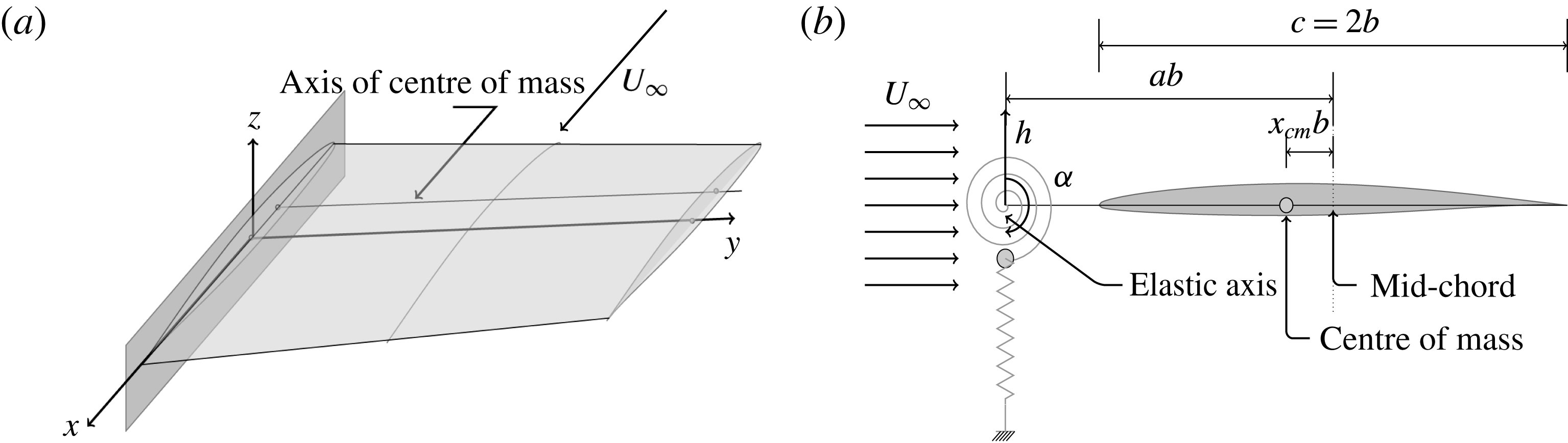
A swept wing shown in figure 1(a) executes a combination of bending and torsional oscillations during flutter. Any section of this wing, assuming the cross-section to be rigid, essentially executes translational vibrations in the
 $z$
-direction and rotational vibrations about the
 $y$
-axis. These motion are referred to as heave and pitch, respectively, in the literature on aeroelasticity. These are depicted in figure 1(b) together with other parameters that define the airfoil motion kinematics. The heave and pitch degrees of freedom are constrained by linear springs. The structural properties of the two-dimensional aeroelastic system such as spring stiffness, mass, moment of inertia, position of the elastic axis and mass centre are chosen such that the airfoil mimics the wing when its motion is dominated by its first two natural modes of oscillation. The airfoil is placed in a flow of uniform velocity in the transonic regime. An initial disturbance to this two-dimensional aeroelastic configuration can lead to net energy extraction from the flow leading to a diverging self-sustained oscillations of the elastic wing section; or net energy loss to the flow that results in decaying wing oscillations; and finally a net energy balance in which the elastic solid neither loses nor gains energy from the flow in one cycle, resulting in sustained periodic oscillations of the wing, and this is usually referred to as aeroelastic flutter.
Aeroelastic configuration (Isogai Reference Isogai1979). (a) Flow over an elastic wing. (b) Two-dimensional aeroelastic equivalent of the wing.

For this aeroelastic system, the elastic axis and the centre of mass of the airfoil are not co-located. The displacements are measured with reference to the elastic axis. Consequently, there is no elastic coupling, and the elasto-dynamic governing equations are coupled through the inertia terms. The forcing functions comprising the unsteady lift and pitching moment are derived from the flow governing equations. The aeroelastic governing equations of motion are then
 $$\begin{eqnarray}\left.\begin{array}{@{}c@{}}m\ddot{h}-S_{\unicode[STIX]{x1D6FC}}\ddot{\unicode[STIX]{x1D6FC}}+K_{h}h=L,\\ -S_{\unicode[STIX]{x1D6FC}}\ddot{h}+I_{\unicode[STIX]{x1D6FC}}\ddot{\unicode[STIX]{x1D6FC}}+K_{\unicode[STIX]{x1D6FC}}\unicode[STIX]{x1D6FC}=M_{ea}.\end{array}\right\}\end{eqnarray}$$
Here
 $L$
and
 $M_{ea}$
are the lift and moment about the elastic axis, with the lift force positive when it is pointing upward and pitching moment positive when oriented nose up.
 $K_{h}$
and
 $K_{\unicode[STIX]{x1D6FC}}$
are the bending and torsional spring stiffnesses.
 $m$
is the mass of the wing per unit span.
 $S_{\unicode[STIX]{x1D6FC}}$
and
 $I_{\unicode[STIX]{x1D6FC}}$
are the static unbalance and the section moment of inertia, respectively, about the elastic axis.
 $h$
and
 $\unicode[STIX]{x1D6FC}$
are the generalized coordinates in plunge and pitch degrees of freedom, with heave positive for upward displacement and pitch positive for nose-up rotation. Non-dimensionalizing time by the natural frequency of the torsional spring,
 $\unicode[STIX]{x1D70F}=\unicode[STIX]{x1D714}_{\unicode[STIX]{x1D6FC}}t$
, we have the governing equations in the form of
 $$\begin{eqnarray}\left[M\right]\left\{q^{\prime \prime }\right\}+\left[K\right]\left\{q\right\}=\left\{F\right\},\end{eqnarray}$$
where
 $$\begin{eqnarray}\left[M\right]=\left[\begin{array}{@{}cc@{}}1 & -x_{\unicode[STIX]{x1D6FC}}\\ -x_{\unicode[STIX]{x1D6FC}} & r_{\unicode[STIX]{x1D6FC}}^{2}\end{array}\right],\quad \left[K\right]=\left[\begin{array}{@{}cc@{}}\left({\displaystyle \frac{\unicode[STIX]{x1D714}_{h}}{\unicode[STIX]{x1D714}_{\unicode[STIX]{x1D6FC}}}}\right)^{2} & 0\\ 0 & r_{\unicode[STIX]{x1D6FC}}^{2}\end{array}\right],\end{eqnarray}$$
are the non-dimensional mass and stiffness matrices,
 $x_{\unicode[STIX]{x1D6FC}}$
is the non-dimensional distance between the mass centre and the elastic axis and is positive when the mass centre is aft of the elastic axis,
 $r_{\unicode[STIX]{x1D6FC}}$
is the radius of gyration with respect to the elastic axis, and
 $\unicode[STIX]{x1D714}_{h}$
and
 $\unicode[STIX]{x1D714}_{\unicode[STIX]{x1D6FC}}$
are the uncoupled natural frequencies of the system in plunge and pitch respectively. The load and displacement vectors are
 $$\begin{eqnarray}\displaystyle \left[F\right]={\displaystyle \frac{1}{\unicode[STIX]{x03C0}\unicode[STIX]{x1D707}\unicode[STIX]{x1D705}^{2}}}\left[\begin{array}{@{}c@{}}C_{l}\\ 2C_{m}\end{array}\right],\quad \left\{q\right\}=\left\{\begin{array}{@{}c@{}}{\displaystyle \frac{h}{b}}\\ \unicode[STIX]{x1D6FC}\end{array}\right\}. & & \displaystyle\end{eqnarray}$$
Here
 $C_{l}$
and
 $C_{m}$
are the coefficient of lift and coefficient of moment about the elastic axis.
 $b$
is the semi-chord of the airfoil,
 $\unicode[STIX]{x1D705}=\unicode[STIX]{x1D714}_{\unicode[STIX]{x1D6FC}}b/U_{\infty }$
is the reduced frequency defined with respect to
 $\unicode[STIX]{x1D714}_{\unicode[STIX]{x1D6FC}}$
,
 $\unicode[STIX]{x1D707}=m/\unicode[STIX]{x03C0}\unicode[STIX]{x1D70C}b^{2}$
is the mass ratio and
 $m$
is airfoil mass per unit span. Equation (2.2) is written in state space form and then numerically integrated using a second-order accurate implicit time integration. These equations are solved for the displacement and velocity vectors.
The aerodynamic terms
 $C_{l}$
and
 $C_{m}$
are computed using a RANS equation using a Spalart–Allmaras turbulence model for closure. A finite volume approach is used for the spatial discretization of the integral form of the governing equations as it satisfies discrete conservation which is necessary for accurate flow computation. Roe’s (Roe Reference Roe1981) approximate Riemann solver is used for the spatial discretization of the convective part of density weighted time-averaged Navier–Stokes equations. The monotone upstream-centred scheme for conservation laws proposed by van Leer (Reference van Leer1979) is used to achieve second-order accurate spatial discretization in smooth regions of flow. The van Albada limiter (Hirsch Reference Hirsch1994, chap. 21) is used for shock resolution without oscillations. Viscous terms are treated using second-order accurate central-difference scheme.
A second-order accurate implicit time discretization of the flow governing equations is carried out. A relaxation scheme which uses the lower–upper implicit factorization proposed by Jameson & Turkel (Reference Jameson and Turkel1981) is implemented for steady flow computations. An implicit dual time stepping is performed for the unsteady flow computations which solves the algebraic equations obtained from both spatial and temporal discretization as a steady flow problem using the relaxation technique in pseudo-time.
Special care is required while discretizing the turbulence model equation (Spalart & Allmaras Reference Spalart and Allmaras1992) taking the stability of the numerical scheme into account. The turbulence equation is decoupled from the Navier–Stokes equation while solving. The advection part is discretized using a first-order accurate upwind scheme. The dissipative term is discretized using a second-order accurate central-difference scheme. To guarantee positivity of the turbulent viscosity variable, the production term is integrated explicitly and the destruction term is integrated implicitly. Lastly, the trip term in the present flow solver is neglected by assuming the free-stream flow to be turbulent.
The fluid velocity on the solid boundary is set equal to the moving solid boundary velocity. The solid wall is assumed adiabatic. The turbulent viscosity is set equal to zero on the solid wall because the Reynolds stresses are zero on the wall. Pressure is extrapolated on the solid surface from the computational domain. Assuming that the flow is subsonic in the free stream, the far-field boundary conditions are imposed using Riemann invariants. At an outflow boundary the tangential velocity and entropy are specified by extrapolation from the computational domain whereas for an inflow boundary they are the free-stream values. These quantities give a complete definition of the flow in the far field. If the flow is supersonic then all the flow quantities are specified as free-stream values at the inflow boundary and are extrapolated at the outflow boundary.
Validation of the flow solver for stationary and oscillating wing sections are presented in appendix A where we have compared inviscid and viscous results with experimental results. In an attached flow, thickness effect of the boundary layer is found to have a significant effect in shifting the shock location and its strength. The computed unsteady lift coefficient, and pressure distribution at different instants for a pitching airfoil, are found to be in good agreement with experimental results. However, there is a qualitative difference in the computed pitching moment coefficient with the experimentally measured ones.
3 The transonic flutter boundary
The test case as given in Isogai (Reference Isogai1979) is considered for the aeroelastic calculations with the following parameters for a NACA 64A010 airfoil section. The non-dimensional distance between the elastic axis and the mass centre is denoted by
 $x_{\unicode[STIX]{x1D6FC}}$
and
 $x_{\unicode[STIX]{x1D6FC}}=1.8$
; the radius of gyration about the elastic axis
 $r_{\unicode[STIX]{x1D6FC}}=\sqrt{3.48}$
; the mass ratio
 $\unicode[STIX]{x1D707}=60$
; the non-dimensional distance between the elastic axis and the mid-chord
 $a=-2.0$
; and the ratio of uncoupled natural frequencies in heave and pitch
 $\unicode[STIX]{x1D714}_{h}/\unicode[STIX]{x1D714}_{\unicode[STIX]{x1D6FC}}=1.0$
. All simulations are performed in a flow of airfoil chord based Reynolds number
 $6\times 10^{6}$
.
A prescribed motion to the airfoil is given through an initial condition. This motion is such that the airfoil is forced in pitching about the elastic axis in the fluid flow, at the given Mach number, for three cycles at a set frequency of
 $\unicode[STIX]{x1D714}_{\unicode[STIX]{x1D6FC}}$
and amplitude
 $1^{\circ }$
. Then the imaginary hinge about which it is pitching is set free and at the same time the forcing too is removed. The time evolution of the aeroelastic system response is then studied.
The computational grids used are of C-type of size
 $256\times 72\times A160$
and the grid spacing on the solid surface is set to
 $y^{+}=1.0$
.
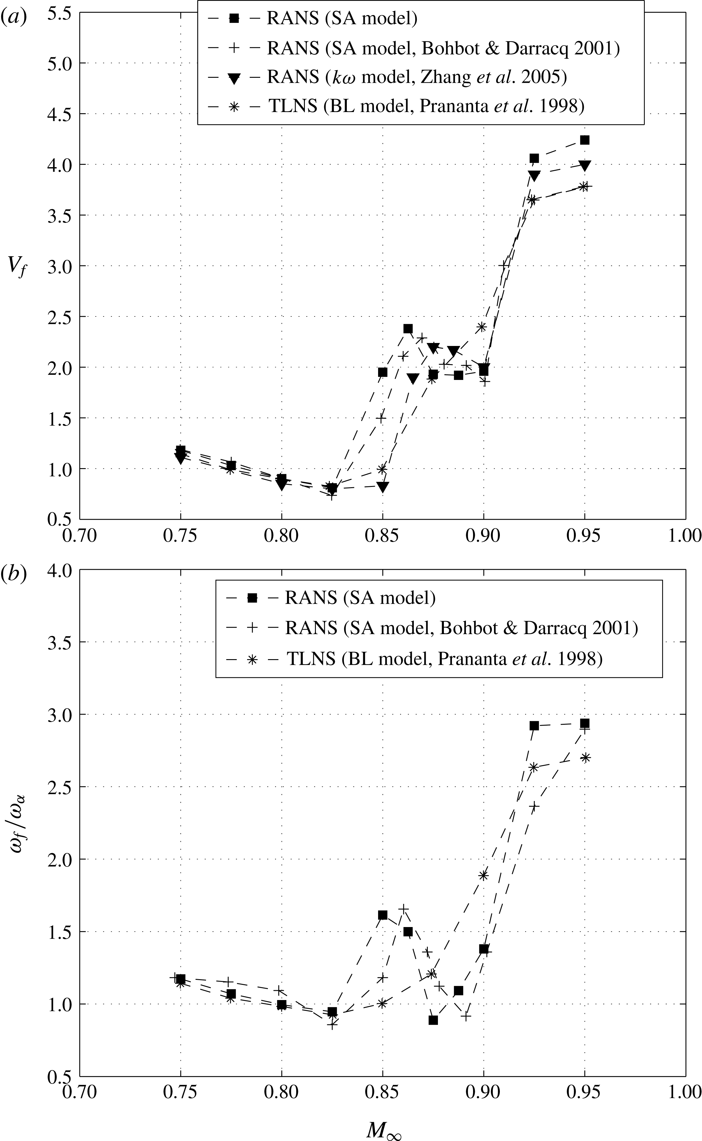
Figure 2(a) shows the comparison of flutter boundary computed by us with those of others using different flow governing equations and different turbulence models that are available in literature. The flutter boundary is a graphical plot of the flutter index and flutter frequency as a function of free-stream Mach number. The flutter index is defined as
 $V_{f}=U_{\infty }/(b\unicode[STIX]{x1D714}_{\unicode[STIX]{x1D6FC}}\sqrt{\unicode[STIX]{x1D707}})$
and denotes the free-stream airspeed with reference to the given flexible lifting surface, at a specified altitude, that gives rise to an undamped oscillation when disturbed from rest. The frequency at which it flutters is called flutter frequency,
 $\unicode[STIX]{x1D714}_{f}$
.
Flutter boundary of the aeroelastic system.

Shown in figure 2(a), Bohbot & Darracq (Reference Bohbot and Darracq2001) numerically solved the RANS equations with the Spalart–Allmaras turbulence model just as we have done. The difference in their flutter boundary and that computed by us could be because of the time integration scheme used for the aeroelastic equations. Bohbot and Darracq used the Newmark method to time integrate the aeroelastic equations whereas we have used a second-order accurate backward-difference scheme to time discretize the set of first-order differential equations in state space form. We have ensured that our flow solver as well as structural dynamic solver uses the same temporal discretization scheme. This also results in reducing the time discretization error due to coupling.
Zhang et al. (Reference Zhang, Yang, Liu and Schuster2005) solved the RANS equations together with the
 $k-\unicode[STIX]{x1D714}$
turbulence model to simulate fluid flow for aeroelastic computations. The flutter boundary computed by Zhang et al. is almost similar to our computation including the peak in the post transonic dip region of
 $0.85\leqslant M_{\infty }\leqslant 0.875$
. But their results under-predict the flutter speed at a given Mach number, and hence the apparent rightward shift. The turbulence model used for the computation may perhaps be the cause of this difference in their and our results. Prananta et al. (Reference Prananta, Hounjet and Zwaan1998) solved the thin-layer Navier–Stokes equations to model the fluid flow for the same aeroelastic system. The Baldwin–Lomax turbulence model was used to model turbulence. The flutter boundary determined by this method does not predict the peak in the region beyond the transonic dip.
The variation of flutter frequency as a function of Mach number, figure 2(b), also shows differences due to different turbulent models that we observed in the flutter boundary results. RANS models capture a similar trend, but the thin-layer Navier–Stokes model is qualitatively different. Thin-layer Navier–Stokes equations are not a good approximation for flows where the streamwise velocity gradients are significant such as near the leading edge and near the shock. In summary, shock and boundary layer interaction computations in the transonic flow regime depends on the governing equations, especially turbulence model used and time integration scheme.
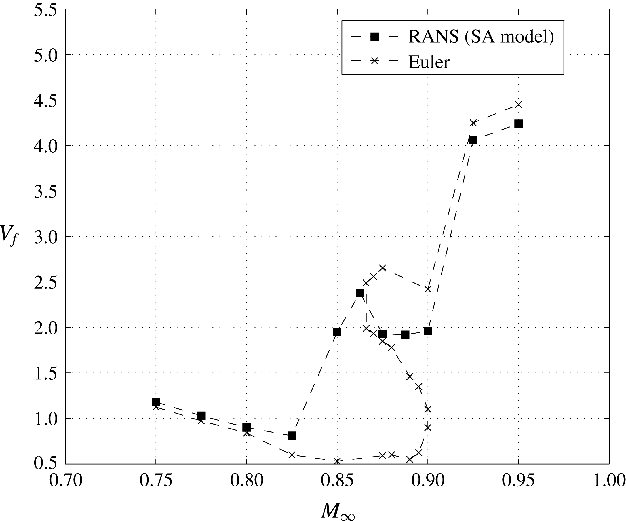
We would like to highlight the comparison of viscous transonic flutter results with those obtained using an inviscid flow solver for the aeroelastic configuration shown in figure 1. The flutter boundary is computed and shown in figures 3 and 4. The flutter boundaries computed by inviscid and viscous solvers are almost the same for
 $M_{\infty }\leqslant 0.825$
and
 $M_{\infty }\geqslant 0.925$
. However in the interval
 $0.825<M_{\infty }<0.925$
the inviscid and viscous solvers predict very different results. For one, the transonic dip is much more pronounced and prolonged until
 $M_{\infty }=0.9$
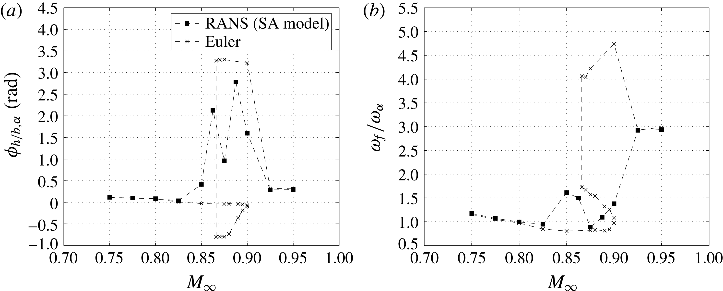
in the inviscid case. The second, and more important feature, is that the viscous flow flutter boundary is remarkable for its absence of multiple flutter points at a given Mach number that is seen in the inviscid results. Even the flutter frequency and phase difference between pitch and heave motions during flutter are significantly different in the transonic flow regime.
In order to better understand the transonic flutter boundary, we first re-visit the transonic flutter similarity parameters of Bendiksen (Reference Bendiksen1998). The similarity parameters are
 $$\begin{eqnarray}\left.\begin{array}{@{}c@{}}\bar{U}={\displaystyle \frac{U_{\infty }}{b\unicode[STIX]{x1D714}_{\unicode[STIX]{x1D6FC}}}},\\ \unicode[STIX]{x1D712}={\displaystyle \frac{1-M_{\infty }^{2}}{\left[(\unicode[STIX]{x1D6FE}+1)M_{\infty }^{2}\unicode[STIX]{x1D6FF}\right]^{2/3}}},\\ \unicode[STIX]{x1D6F9}={\displaystyle \frac{\bar{U}^{2}}{\unicode[STIX]{x03C0}\unicode[STIX]{x1D707}\left[(\unicode[STIX]{x1D6FE}+1)M_{\infty }^{2}\unicode[STIX]{x1D6FF}\right]^{1/3}}}.\end{array}\right\}\end{eqnarray}$$
Comparison of flutter boundary using inviscid and viscous computation.

Flutter frequency and phase difference as a function of Mach number using inviscid and viscous computation: (a) phase difference between
 $-h/b$
and
 $\unicode[STIX]{x1D6FC}$
with
 $M_{\infty }$
; (b)
 $\unicode[STIX]{x1D714}_{f}/\unicode[STIX]{x1D714}_{\unicode[STIX]{x1D6FC}}$
versus
 $M_{\infty }$
.

These similarity parameters are derived using transonic small perturbation equations and as such are merely to be used as pointers that airfoils belonging to the same family having different thickness and flow conditions can be compared using these parameters. The idea being that the response of two aeroelastic systems having the same similarity parameters will give similar flutter response. In the above set of relations,
 $\bar{U}$
is the reciprocal of reduced frequency of oscillation of the aeroelastic system, indicating the requirement that oscillations occur at the same reduced frequency for the two aeroelastic systems. If
 $\unicode[STIX]{x1D712}$
is equal this indicates the similarity of pressure distribution on two airfoil surfaces that are compared under quasi-steady conditions. Lastly,
 $\unicode[STIX]{x1D6F9}$
represents the equivalence of unsteady aerodynamic forces on aeroelastic systems under consideration.
The effect of viscosity for
 $M_{\infty }\leqslant 0.825$
is just to increase the thickness of the airfoil profile for the external flowing fluid as no separation is encountered in these flow regimes. Increased thickness on the airfoil is not the same throughout the airfoil surface. As a first approximation, if we use these similarity parameters to explain the shift in flutter boundary for
 $M_{\infty }\leqslant 0.825$
, we find that the similarity parameters predict that the viscous flutter boundary be placed below the inviscid flutter boundary: this is exactly opposite to the numerical viscous flutter prediction shown in figure 3. This difference is amplified at
 $M_{\infty }=0.825$
.
We now take a look at the flutter phenomenon at four Mach numbers more closely in order to better understand the fluid–elastic interactions as well as explain the deviation from results obtained using inviscid fluid flow models.
 $M_{\infty }=0.825,V_{f}=0.81$

The viscous solver predicts an early, weaker shock compared with the inviscid calculation. The growth of the boundary layer downstream of the shock decreases the streamwise pressure gradient in this region leading to this early, weak shock. It is known that shocks are destabilizing in the transonic dip region. However, the reduced shock strength because of viscosity increases the flutter index or flutter speed in the transonic dip region and is therefore stabilizing. Thus, the effect of thickness increase due to viscosity is the cause of a shallower dip in the transonic region compared to the inviscid flutter boundary. So, in summary, the transonic flutter similarity parameters are really not very useful while predicting trends in the flutter boundary due to viscosity-induced airfoil thickness increase.
Aeroelastic system response and shock displacement at
 $M_{\infty }=0.825$
and
 $V_{f}=0.81$
during a cycle of flutter.

Skin-friction variation on the airfoil surface at different instants for
 $M_{\infty }=0.85$
and
 $V_{f}=1.93$
: (a)
 $\unicode[STIX]{x1D6FC}=0.015^{\circ },h/b=-0.0037,\unicode[STIX]{x1D711}=2.40^{\circ }$
; (b)
 $\unicode[STIX]{x1D6FC}=0.355^{\circ },h/b=-0.0076,\unicode[STIX]{x1D711}=90.23^{\circ }$
; (c)
 $\unicode[STIX]{x1D6FC}=-0.014^{\circ },h/b=0.0037,\unicode[STIX]{x1D711}=182.46^{\circ }$
; (d)
 $\unicode[STIX]{x1D6FC}=-0.353^{\circ },h/b=0.0076,\unicode[STIX]{x1D711}=270.28^{\circ }$
.

The phase difference between heave and pitch degrees of freedom is shown in figure 4(a). A positive phase angle is when heave motion leads the pitching motion. At
 $M_{\infty }=0.825$
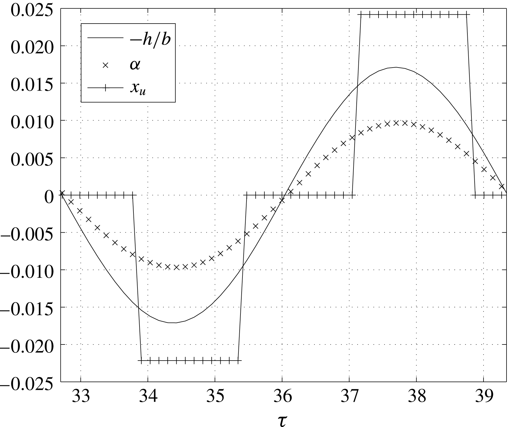
the phase difference is close to zero. The flutter frequency too, figure 4(b), is at its lowest point. The response of the aeroelastic system at this point is predominantly first mode. The flutter frequency is almost equal to the uncoupled natural frequency in pitch. Inviscid flow results too predict almost the same phase difference and flutter frequency. Viscosity seems to have little influence at this point in the transonic flow regime. As shown in figure 5, unsteady shock oscillations –
 $x_{u}(\unicode[STIX]{x1D70F})$
– that are not in phase with the airfoil motion are responsible for the sustained oscillations of the elastic wing.
$M_{\infty }=0.85,V_{f}=1.93$

A sudden increase in flutter speed is observed for
 $0.825\leqslant M_{\infty }\leqslant 0.8625$
in the case of the viscous transonic flutter boundary. We first analyse the case of flutter at
 $M_{\infty }=0.85$
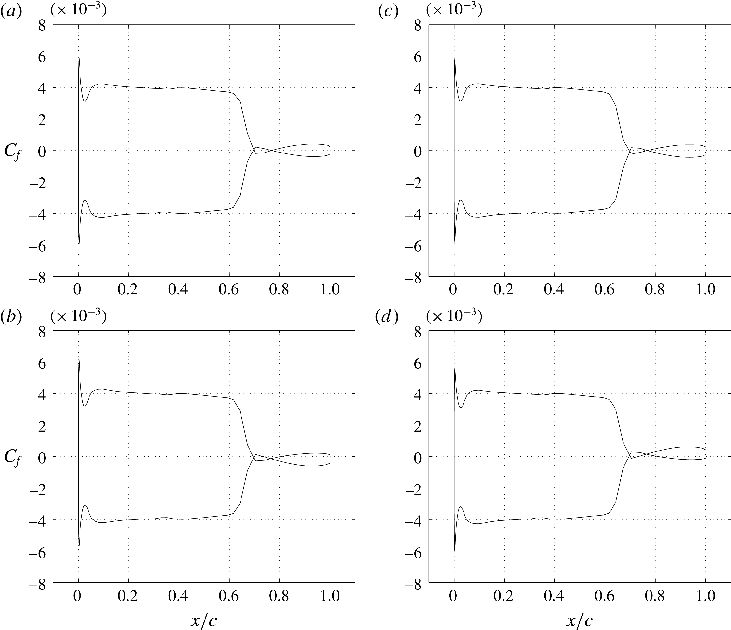
. The increase in Mach number increases the shock strength leading to separation. But the separated region reattaches immediately downstream. In figure 6 the skin-friction distribution on the airfoil surface at different instants, measured in terms of the phase
 $\unicode[STIX]{x1D711}=\unicode[STIX]{x1D714}_{f}t$
of the pitch oscillation during a cycle of flutter, is shown. The skin friction distribution on the upper and lower surface crosses the zero skin-friction line twice indicating separation and reattachment. In fact the shock-induced separation and reattachment has a significant effect on the flutter boundary and is reflected in figures 3 and 4. Further, in this case the effect of viscosity is not restricted just to increase the airfoil profile thickness with reference to the external fluid flow.
It can be seen from the phase difference plot, figure 4(a) at
 $M_{\infty }=0.85$
, that the phase difference between the two degrees of freedom of the aeroelastic system increases. It is possible that the flow separation and re-attachment over the airfoil surface leads to changing the aerodynamic damping perceived by the aeroelastic oscillator. This in turn induces, one, a phase difference between the shock and airfoil motion; and two, increases the phase difference between heave and pitch degrees of freedom leading to an increase in aerodynamic coupling for the extraction of energy from the flow. The combination of these influences results in increasing the flutter index at
 $M_{\infty }=0.85$
, on the flutter boundary, relative to that at
 $M_{\infty }=0.825$
.
$M_{\infty }=0.875,V_{f}=1.93$

Figure 7 shows the flutter response at
 $M_{\infty }=0.875$
with a flutter index
 $V_{f}=1.93$
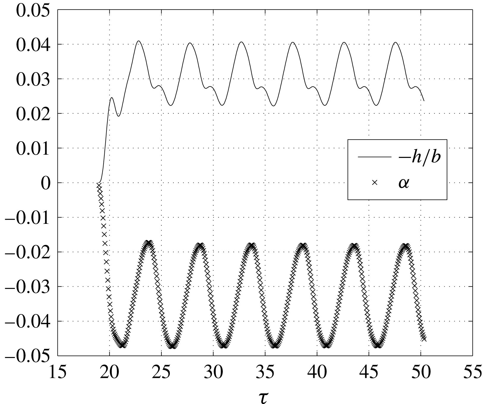
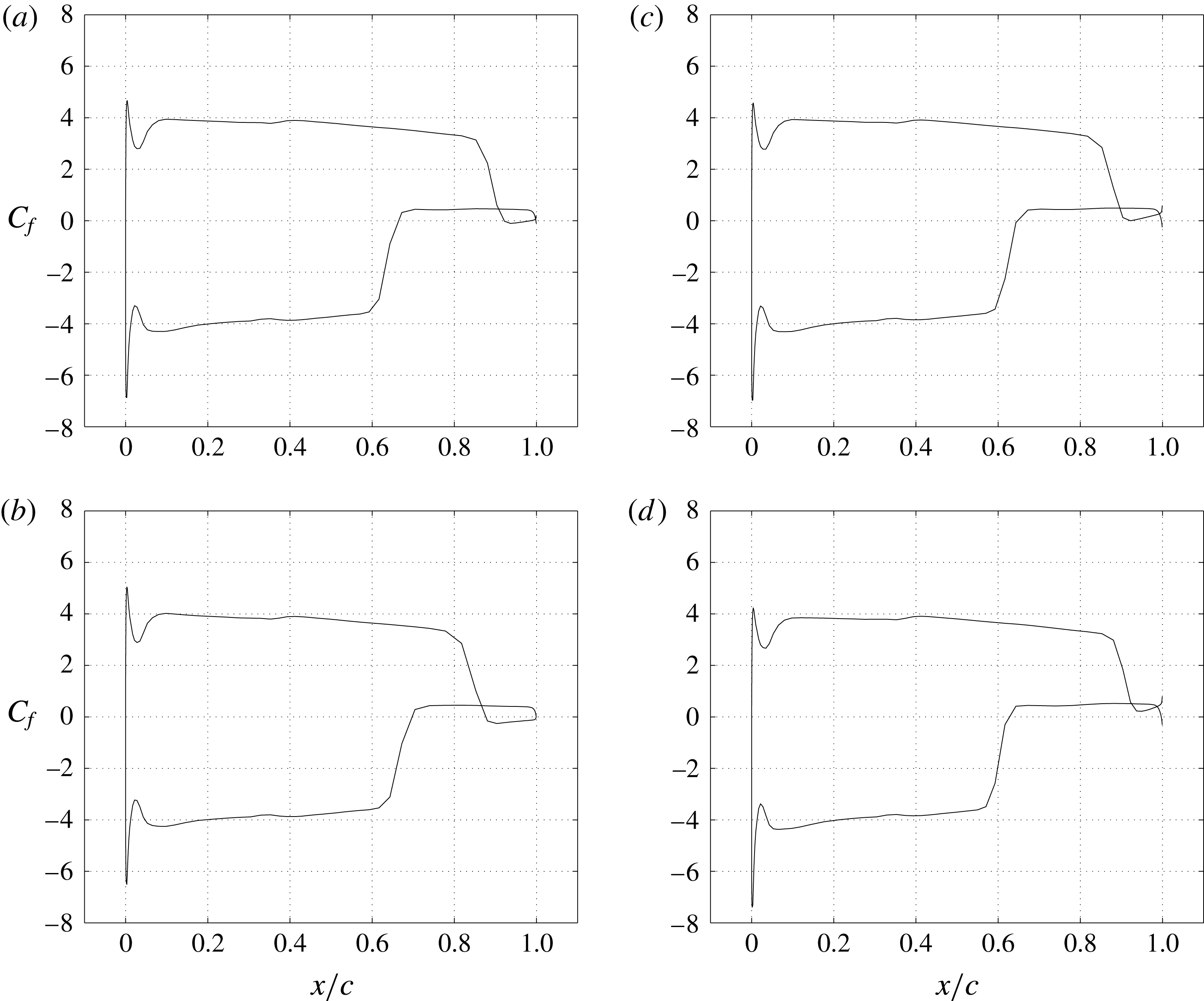
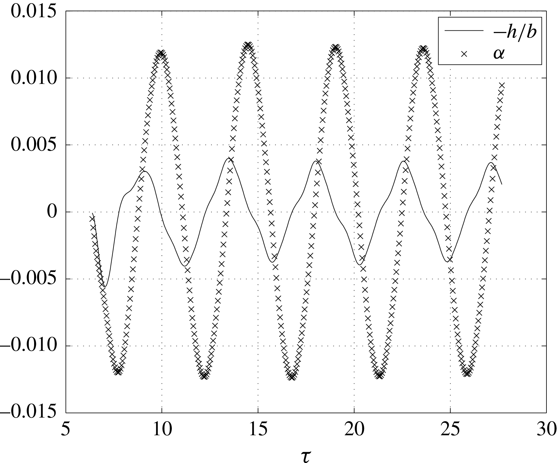
. The response shows the system oscillating about a new equilibrium position that is vertically displaced upward and with a nose down attitude. The increase in Mach number increases the shock strength on the airfoil surface leading to separation of the fluid on the airfoil surface. That this is so can be observed and verified in the skin-friction distribution shown in figure 8. Because of the large pressure rise in the separated region on the lower surface of the airfoil, the airfoil is pushed up with its nose down. The elastic forces are unable to recover the system to its original equilibrium position.
Aeroelastic system response for
 $M_{\infty }=0.875$
and
 $V_{f}=1.93$
.

Skin-friction variation on the airfoil surface at different instants for
 $M_{\infty }=0.875$
and
 $V_{f}=1.93$
. (a)
 $\unicode[STIX]{x1D6FC}=-1.72^{\circ },h/b=-0.040,\unicode[STIX]{x1D711}=0.11^{\circ }$
(b)
 $\unicode[STIX]{x1D6FC}=-1.03^{\circ },h/b=-0.032,\unicode[STIX]{x1D711}=85.79^{\circ }$
. (c)
 $\unicode[STIX]{x1D6FC}=-2.07^{\circ },h/b=-0.027,\unicode[STIX]{x1D711}=171.47^{\circ }$
. (d)
 $\unicode[STIX]{x1D6FC}=-2.69^{\circ },h/b=-0.023,\unicode[STIX]{x1D711}=257.15^{\circ }$

Mach contours at different instants for
 $M_{\infty }=0.875$
and
 $V_{f}=1.93$
: (a)
 $\unicode[STIX]{x1D6FC}=-1.72^{\circ },h/b=-0.040,\unicode[STIX]{x1D711}=0.11^{\circ }$
; (b)
 $\unicode[STIX]{x1D6FC}=-1.03^{\circ },h/b=-0.032,\unicode[STIX]{x1D711}=85.79^{\circ }$
; (c)
 $\unicode[STIX]{x1D6FC}=-2.07,h/b=-0.027,\unicode[STIX]{x1D711}=171.47^{\circ }$
; (d)
 $\unicode[STIX]{x1D6FC}=-2.69,h/b=-0.023,\unicode[STIX]{x1D711}=257.15^{\circ }$
.

Pressure distribution on the airfoil surface at different instants for
 $M_{\infty }=0.875$
and
 $V_{f}=1.93$
: (a)
 $\unicode[STIX]{x1D6FC}=-1.72^{\circ },h/b=-0.040,\unicode[STIX]{x1D711}=0.11^{\circ }$
; (b)
 $\unicode[STIX]{x1D6FC}=-1.03^{\circ },h/b=-0.032,\unicode[STIX]{x1D711}=85.79^{\circ }$
; (c)
 $\unicode[STIX]{x1D6FC}=-2.07,h/b=-0.027,\unicode[STIX]{x1D711}=171.47^{\circ }$
; (d)
 $\unicode[STIX]{x1D6FC}=-2.69,h/b=-0.023,\unicode[STIX]{x1D711}=257.15^{\circ }$
.

Phase plane plots of heave and pitch degrees of freedom for
 $M_{\infty }=0.875$
and
 $V_{f}=1.93$
for different initial conditions: (a) phase plane plot of heave motion; (b) phase plane plot of pitch motion.

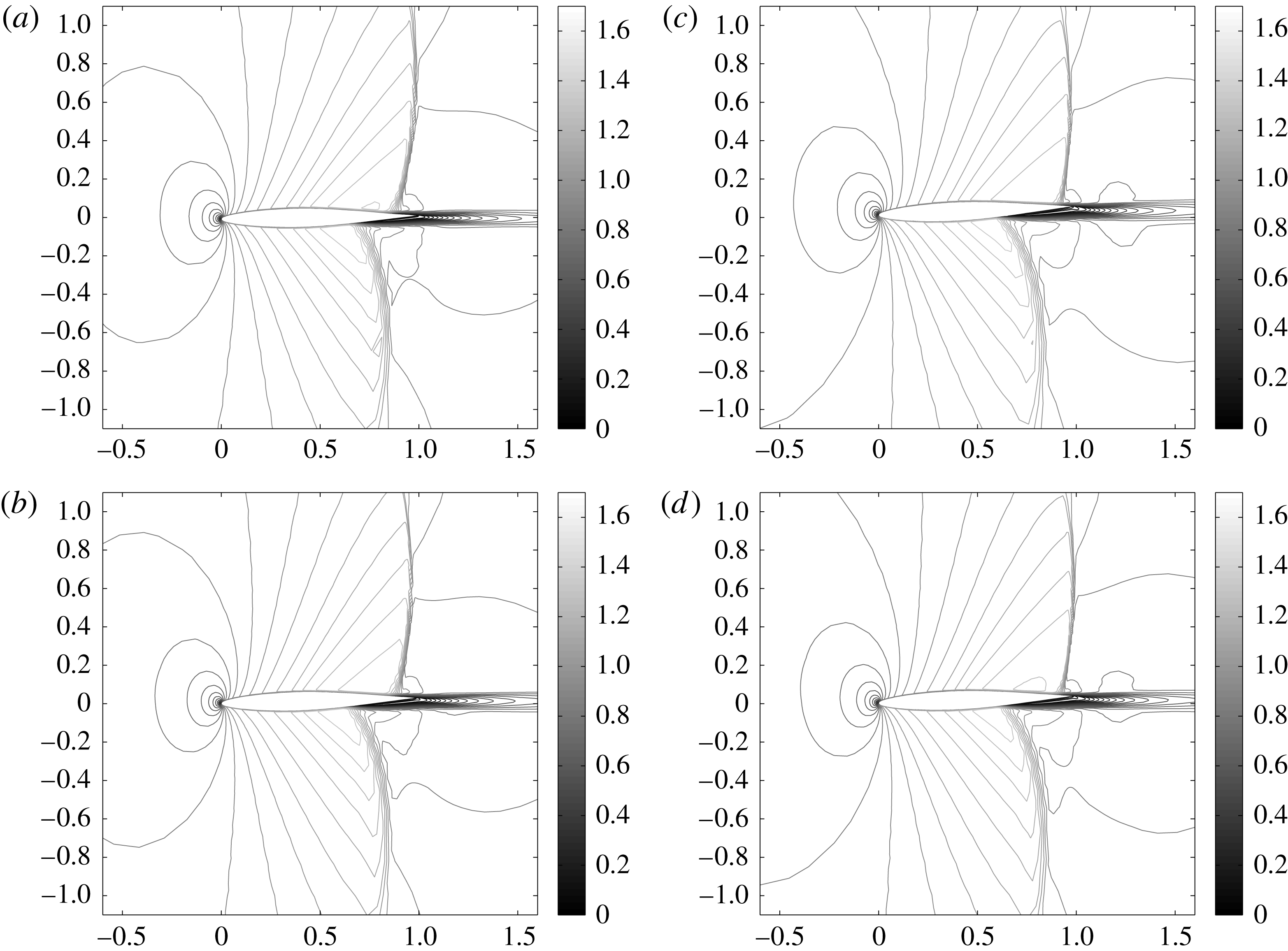
The Mach contours shown at these instants in figure 9 give a clearer picture of what is taking place. Note that the shock on the upper surface occurs aft relative to that on the lower surface of the airfoil. Since the airfoil’s new equilibrium position is nose down throughout the oscillation cycle, the shock on the lower surface separates the flow much earlier than the upper surface shock. The nose down position during all the instants is expected to give a stronger shock on the lower surface of the airfoil if the fluid were inviscid. But the boundary layer being unable to sustain the pressure gradient separates much earlier pushing the shock upstream with reduced strength. Supplementary movie 1 showing Mach contours of the flutter response at
 $M_{\infty }=0.875$
and
 $V_{f}=1.93$
using RANS simulation can be found at https://doi.org/10.1017/jfm.2017.629. For comparison, we have also shown the Euler simulations of the flutter response at
 $M_{\infty }=0.875$
and
 $V_{f}=1.85$
in supplementary movie 2.
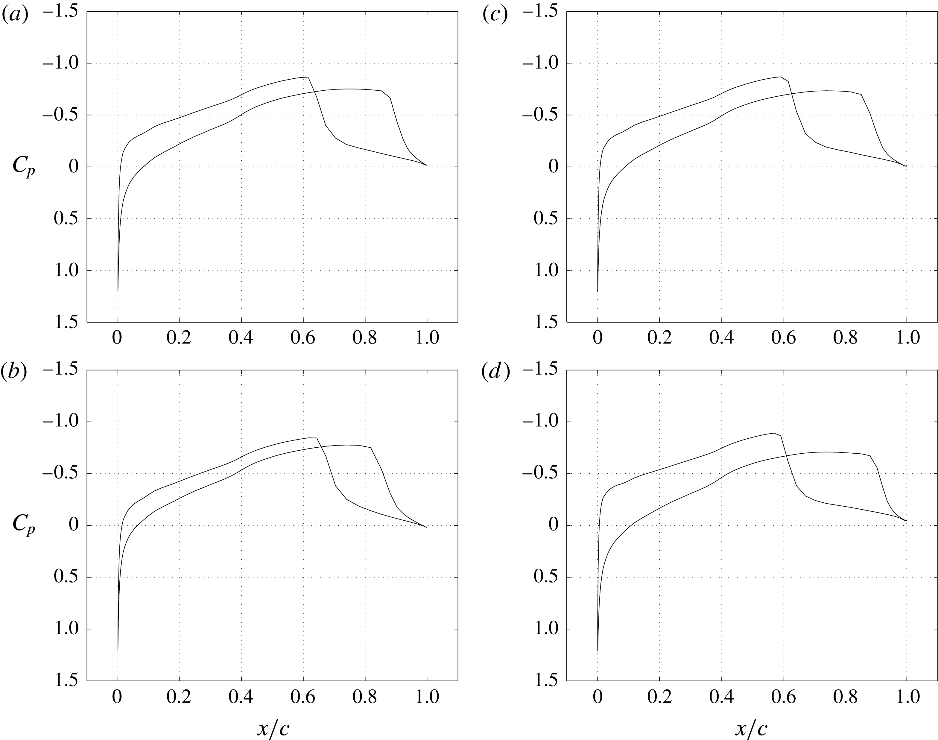
We have also shown the pressure distribution on the airfoil surface at different instants of the flutter cycle of figure 10 that gives a better idea of the pressure induced on the upper and lower surface of the airfoil as a consequence of the shock-induced boundary layer separation. On the lower surface of the airfoil, shock occurs much earlier than on the upper surface. Therefore, the post shock region for the lower surface is larger compared to that of the upper surface. This leads to displacing the wing upwards and giving it a nose down attitude in pitch.
Note that the coefficient of pressure on the upper and lower surfaces are negative, or denote suction, and that the shock is stronger on the lower surface. Flow separation, induced by the shock, too occurs earlier along the chord on the lower airfoil surface. The suction pressure is responsible for displacing the wing upward and giving it a nose down attitude in pitch.
As a consequence of all these complex flow phenomena, a sudden change in trend is observed in the flutter boundary shown in figures 3 and 4 for
 $M_{\infty }=0.875$
with a flutter index
 $V_{f}=1.93$
. The flutter index and flutter frequency drops relative to that at
 $M_{\infty }=0.8625$
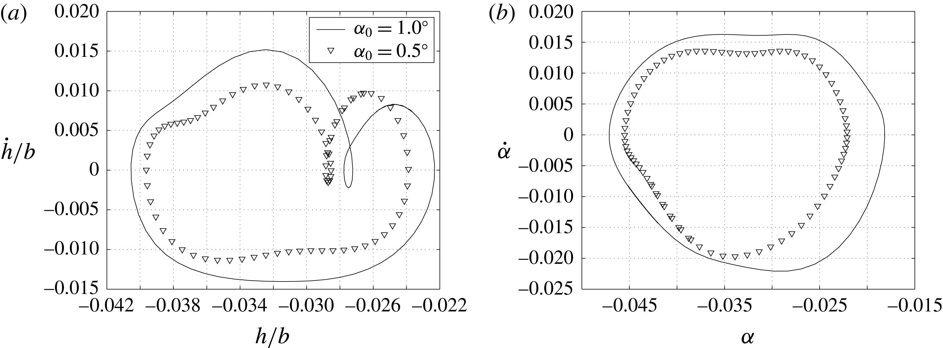
making the elastic system more vulnerable to flutter. We also investigated the influence of initial conditions in order to ascertain if the oscillations were of the limit-cycle type. The existence of a periodic equilibrium solution is implied by the response in the state space being independent of initial conditions. The phase plane plots for the heave and pitch degrees of freedom for different initial conditions are shown in figure 11. It can be seen that unlike in the case of limit-cycle oscillations that are independent of initial conditions, the flutter response of the system depends on the initial condition.
$M_{\infty }=0.9,V_{f}=1.950$

With further increase in Mach number the shock strength increases and at the same time the shock is pushed further downstream towards the trailing edge. We consider the specific case of
 $M_{\infty }=0.900$
to discuss some of the features in this regime. This shock leads to separation but the separated region is much smaller than at
 $M_{\infty }=0.875$
and hence the elastic forces bring back the system to oscillate about its original equilibrium position unlike the previous case. Figure 12 shows the response of the aeroelastic system where the amplitude of pitching is higher than the amplitude of heaving. The separated region near the trailing edge, even though restricted to a small region because of its large moment arm, imparts a greater moment leading to a response with large pitching amplitude.
$M_{\infty }=0.925,V_{f}=4.0,M_{\infty }=0.95,V_{f}=4.25$

Now, finally, we consider flutter at two flight Mach numbers:
 $M_{\infty }=0.925$
and
 $M_{\infty }=0.950$
. The increase in Mach number pushes the shock to the trailing edge of the airfoil and hence the effect of viscosity on the flutter boundary is completely eliminated. The flutter boundary computed by inviscid and viscous solutions almost coincide in these cases. This can be seen in the flutter boundary at these two Mach numbers in figures 3 and 4. The boundary layer thickness effect is negligibly small as the flow is accelerating throughout the surface of the airfoil. Whatever differences are observed in the viscous and inviscid flutter boundary are perhaps due to numerical errors arising from the choice of C-grids used for viscous computations and O-grids used for inviscid computations.
Aeroelastic system response for
 $M_{\infty }=0.900$
and
 $V_{f}=1.950$
.

We can now consolidate and summarize the above discussion. Until the bottom of the transonic dip or
 $M_{\infty }\leqslant 0.825$
, the influence of viscosity, through the boundary layer, is an apparent increase in the thickness of the airfoil that pushes the flutter boundary towards higher flutter indices and as such tends to augment the stability of the aeroelastic system. A further increase in Mach number beyond the bottom of the flutter boundary,
 $0.825<M_{\infty }<0.8625$
, the presence of shocks on both bottom and top surfaces leads to separation and subsequent re-attachment on the respective surfaces. This leads to a sudden increase in the flutter boundary. An increase in shock strength because of further increase in free-stream Mach number,
 $M_{\infty }=0.875$
, leads to separation of the flow inducing the system to oscillate about a new equilibrium position. This is accompanied by a sudden drop in the flutter boundary thereby destabilizing the aeroelastic system. This is the region where viscosity significantly changes the flutter boundary and the nature of fluid–elastic interaction in transonic flow because of shock-induced separation. A further increase in Mach number,
 $M_{\infty }\geqslant 0.925$
, pushes the shock to the trailing edge; the influence of shock and shock boundary layer interaction is minimal, and the flutter boundary trends similarly with the inviscid flutter boundary of the aeroelastic system. In this region viscous effects have no significant effect on the flutter characteristics of the aeroelastic system considered.
4 Shock–boundary layer interaction and energetics
Rearranging the aeroelastic governing equation (2.2) for the net energy input into the structure gives
 $$\begin{eqnarray}\int _{0}^{T}\{F\}\{q^{\prime }\}\,\text{d}\unicode[STIX]{x1D70F}=\int _{0}^{T}[[M]\{q^{\prime \prime }\}+[K]\{q\}]\{q^{\prime }\}\,\text{d}\unicode[STIX]{x1D70F}.\end{eqnarray}$$
When there is no net energy input into the structure during one cycle of oscillation, then the amplitude of oscillation remains constant, and the aeroelastic system is said to be in a state of flutter. If the elastic structure accumulates energy, the amplitude of oscillations of the structure increases and the structure may eventually fail. Instead, if the structure loses energy to the flowing fluid around it in every cycle of oscillation, then the aeroelastic system oscillates with diminishing amplitude in every cycle and reaches a stable equilibrium position.
In terms of stored energy of the structure, the above equation can be written as
 $$\begin{eqnarray}\int _{0}^{T}\left[K\right]\left\{q\right\}\left\{q^{\prime }\right\}\,\text{d}\unicode[STIX]{x1D70F}=\int _{0}^{T}\left[\left\{F\right\}-\left[M\right]\left\{q^{\prime \prime }\right\}\right]\left\{q^{\prime }\right\}\,\text{d}\unicode[STIX]{x1D70F}.\end{eqnarray}$$
This stored energy of the system will give a measure for the variation of net energy of the aeroelastic system.
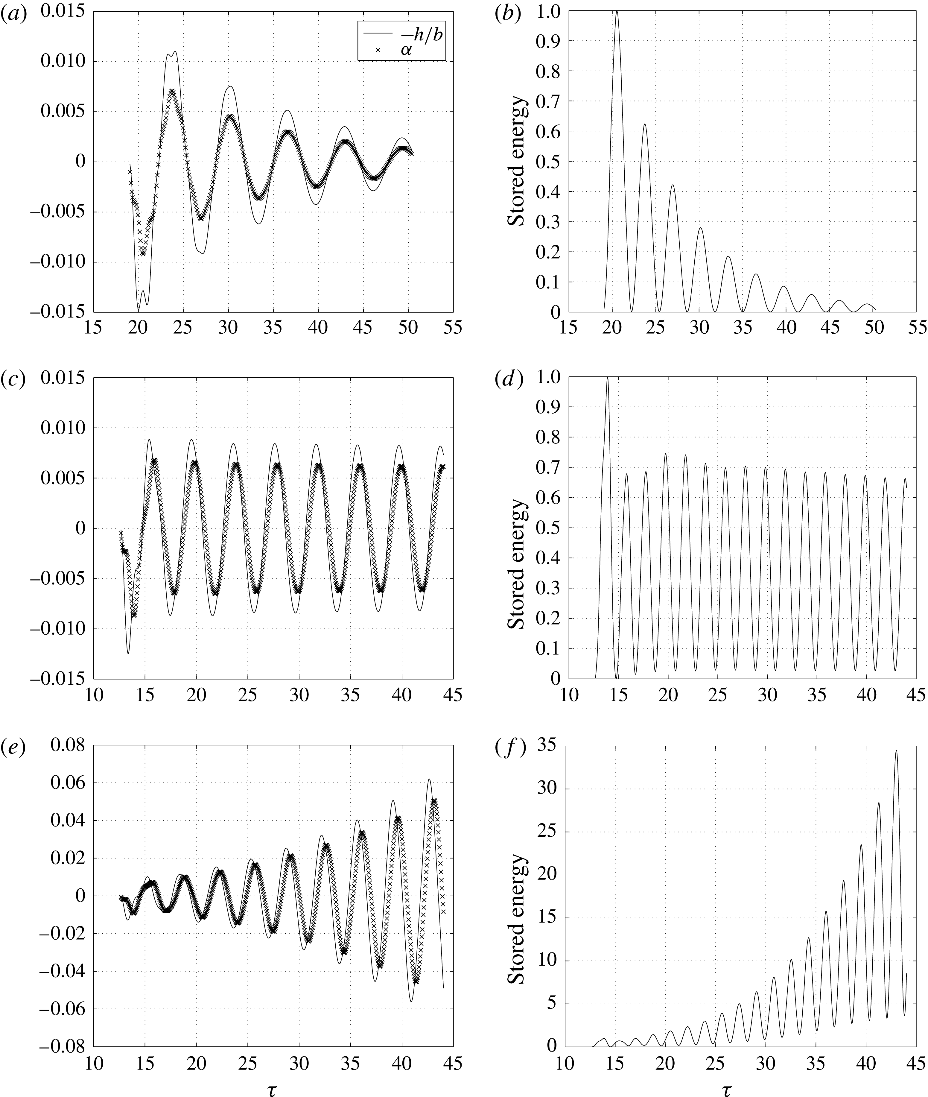
In figure 13, we illustrate these three cases of the aeroelastic system response corresponding to three different airspeeds
 $V_{f}$
for a Mach number of
 $M_{\infty }=0.85$
. Note that at this Mach number the aeroelastic system flutters at
 $V_{f}=1.93$
. Figure 13(a,c,e) presents the aeroelastic system response in terms of the time history of heave and pitch degrees of freedom, and figure 13(b,d,f) the variation of the stored elastic energy in the aeroelastic system. In figure 13(a,b)
 $V_{f}=1.00$
and is less than the flutter speed
 $V_{f}=1.93$
, and consequently, the amplitude of oscillation decreases and the stored energy in the aeroelastic also decays. When
 $V_{f}=1.93$
, the stored energy does not change after every cycle of oscillation shown in figure 13(d), and the system is executing a neutral response shown in figure 13(c). If the system starts accumulating energy, as when
 $V_{f}=2.30$
, the system executes a diverging response and the stored energy after every cycle increases as shown in 13(e) and 13(f) respectively.
In (4.2),
 $\{F\}\left\{q\prime \right\}$
is the aerodynamic power transferred to the elastic wing by fluid forces. In the discussion that follows we study the effect of viscosity in changing the power distribution on the surface of the wing section at airspeeds where flutter occurs. The net energy input to the wing is zero.
Different flutter response and stored energy of the aeroelastic system at
 $M_{\infty }=0.850$
: (a) damped response at
 $V_{f}=1.00$
; (b) stored energy variation at
 $V_{f}=1.00$
; (c) neutral response at
 $V_{f}=1.93$
; (d) stored energy variation at
 $V_{f}=1.93$
; (e) diverging response at
 $V_{f}=2.30$
; (f) stored energy variation at
 $V_{f}=2.30$
.

The aerodynamic power calculated on the surface of the airfoil due to two forces, namely pressure and viscous forces are
 $$\begin{eqnarray}\left.\begin{array}{@{}c@{}}\text{aerodynamic power due to pressure force}_{x,z}=(\unicode[STIX]{x0394}zx^{\prime }-\unicode[STIX]{x0394}xz^{\prime })p,\\ \text{aerodynamic power due to viscous force}_{x,z}=(\unicode[STIX]{x0394}xx^{\prime }+\unicode[STIX]{x0394}zz^{\prime })\frac{1}{2}\unicode[STIX]{x1D70C}_{\infty }u_{\infty }^{2}C_{f}.\end{array}\right\}\end{eqnarray}$$
Here
 $\unicode[STIX]{x0394}x$
and
 $\unicode[STIX]{x0394}z$
are the increments in
 $x$
and
 $z$
directions on the airfoil surface over which the pressure
 $p$
and skin friction coefficient
 $C_{f}$
are computed numerically.
 $x^{\prime }$
and
 $z^{\prime }$
are the velocities in
 $x$
and
 $z$
directions respectively on the airfoil surface at point
 $(x,z)$
. The computed power at each point
 $(x,z)$
is non-dimensionalized by
 $\unicode[STIX]{x1D70C}_{\infty }b^{5}\unicode[STIX]{x1D714}_{\unicode[STIX]{x1D6FC}}^{3}$
. The total power is defined as the power applied on the camber line of the airfoil and is equal to the sum of the power on the upper and lower surfaces corresponding to the points on the camber line. We focus our attention on the flutter phenomenon at two Mach numbers:
 $M_{\infty }=0.825$
and
 $M_{\infty }=0.875$
. As discussed earlier, at
 $M_{\infty }=0.825$
there is sudden increase in the flutter speed attributed to separation and re-attachment; at
 $M_{\infty }=0.875$
flutter oscillations occur about a new equilibrium position displaced upward and pitching nose-down due to shock-induced flow separation on the top and bottom airfoil surfaces.
$M_{\infty }=0.825$

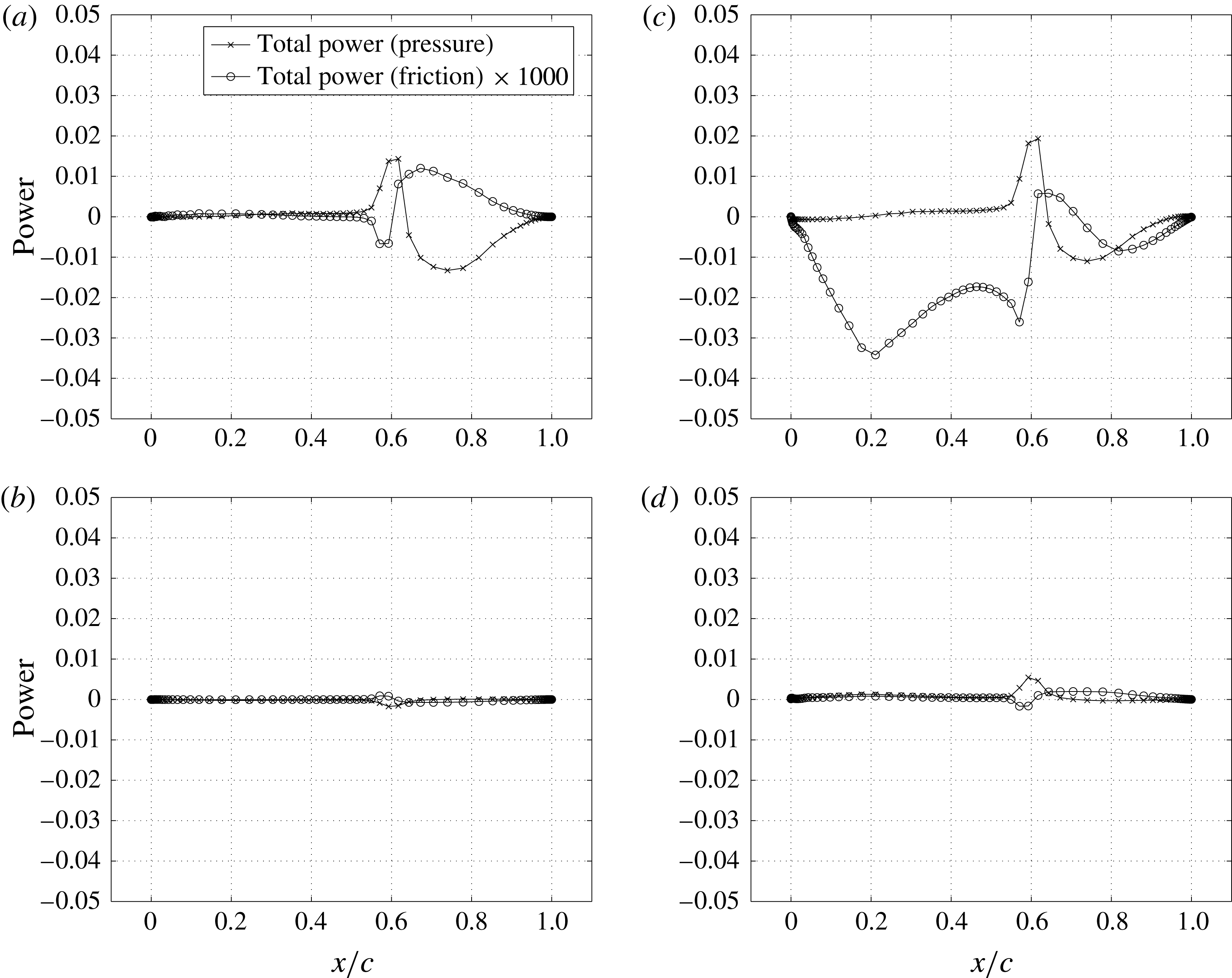
Figure 14 shows total power variation on the airfoil camber line at different instants of flutter at the bottom of the transonic dip at
 $M_{\infty }=0.825$
and
 $V_{f}=0.810$
. This is the case of predominant single mode oscillations of the aeroelastic system as discussed in the context of figures 4 and 5 in § 3. Power distributions in figure 14(b,d) show zero power contribution by aerodynamic forces as the velocity become zero at these instants. Power contribution by viscous forces is very small, almost three orders of magnitude less compared to pressure forces. The power contribution by shocks due to pressure forces is always positive, indicating the unsteady shock motion being responsible for the sustained oscillations of the system. We have observed this in the inviscid case at the same Mach number too. But because of viscous effects, shocks are less strong and are diffused at their feet. This leads to a lower power contribution to the elastic system by the shocks. However, unlike in the inviscid simulations though, power in the region downstream of the shock is negative indicating that viscous effects extract energy from the system and make it more stable.
$M_{\infty }=0.875$

The flutter response of the aeroelastic system at
 $M_{\infty }=0.875$
is interesting for many reasons. In the viscous simulations, the system flutters about a new equilibrium position accompanied by a local minimum of the flutter boundary. In the inviscid simulations, multiple flutter points are observed at
 $M_{\infty }=0.875$
, as seen in figure 3. Now if one were to examine the phase difference between the two degrees of freedom at this Mach number, shown in figure 4(a), for the viscous simulations there is significant phase difference: around
 $1$
radian or
 $57.3^{\circ }$
. The inviscid simulations shows that the phase difference changes at each of the three flutter speeds. At
 $V_{f}=0.592$
the phase difference is close to zero,
 $-0.0386$
, and the motion is predominantly first mode; at
 $V_{f}=1.850$
the phase difference is
 $-0.7347$
implying that heaving motion lags pitch but there is contribution from first and second modes of oscillation; and at
 $V_{f}=2.654$
, the phase difference is
 $3.3$
or close to
 $\unicode[STIX]{x03C0}$
, the heave and pitch motions are
 $180^{\circ }$
out of phase with each other, and the response is predominantly second mode. In other words, one observes here a case of multiple flutter speeds at a given Mach number, with increasing phase difference as the flutter speed increases, and varied modal participation in the flutter response.
Power distribution on the airfoil surface at different instants for
 $M_{\infty }=0.825$
and
 $V_{f}=0.810$
: (a)
 $\unicode[STIX]{x1D6FC}=0.02^{\circ },h/b=-0.001,\unicode[STIX]{x1D711}=2.83^{\circ }$
; (b)
 $\unicode[STIX]{x1D6FC}=0.55^{\circ },h/b=-0.017,\unicode[STIX]{x1D711}=88.01^{\circ }$
; (c)
 $\unicode[STIX]{x1D6FC}=0.02^{\circ },h/b=0.00,\unicode[STIX]{x1D711}=180.29^{\circ }$
; (d)
 $\unicode[STIX]{x1D6FC}=-0.55^{\circ },h/b=0.017,\unicode[STIX]{x1D711}=272.57^{\circ }$
.

At
 $M_{\infty }=0.875$
the flutter frequency
 $\unicode[STIX]{x1D714}_{f}/\unicode[STIX]{x1D714}_{\unicode[STIX]{x1D6FC}}=0.71$
as seen in figure 4(b). This fundamental frequency of the flutter response is close to the first mode frequency. Notice that the inviscid simulations at this Mach number show multiple flutter frequencies corresponding to multiple flutter speeds, but at each of these flutter speeds the flutter response has a predominant single frequency component. The frequency of flutter response increases as the flutter speed increases and moves from the first mode natural frequency to the second mode natural frequency; the second mode participation increases with increase in flutter frequency and flutter speed.
Phase plane plot for
 $M_{\infty }=0.875$
flutter case: (a) first mode; (b) second mode.

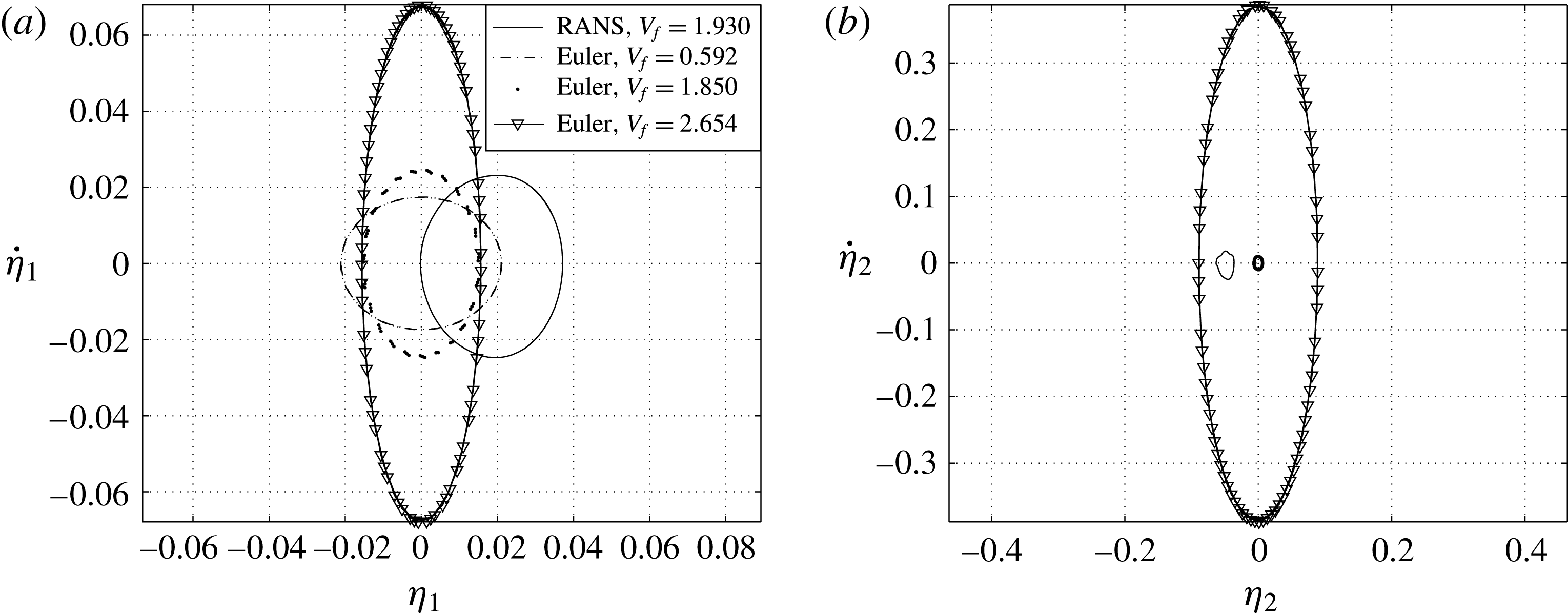
The phase plane plots in terms of modal coordinates for the aeroelastic system at
 $M_{\infty }=0.875$
are shown in figure 15. Here
 $\unicode[STIX]{x1D702}_{1}$
and
 $\unicode[STIX]{x1D702}_{2}$
are the first and second mode of the aeroelastic system. Both viscous and inviscid Euler results are included in these plots. The phase plane plots in terms of modal coordinates give a rough idea of the relative contribution by different modes to the response of the aeroelastic system during flutter. The first mode contribution to the flutter response is shown in figure 15(a). The first mode contribution to the response in the viscous and inviscid simulations are comparable. The viscous simulations shows the first mode oscillations about a new equilibrium point that is displaced vertically upward and nose-down, this was discussed earlier with reference to figure 7, and the first mode response re-affirms that observation. The contribution of the second mode to the overall response is shown in figure 15(b). The second mode oscillations computed from the viscous simulations are also about the new equilibrium position as shown in figure 7. The second mode contribution to the flutter response points to a significant variation between the RANS and inviscid simulations. At the three flutter speeds in the inviscid simulations at this Mach number, the second mode contribution is significantly different not only with reference to that of the viscous simulations but also between each other. The inviscid flutter response varies: starting from first mode flutter at the lowest flow speed
 $V_{f}=0.592$
, it jumps to binary flutter involving coupling between modes at
 $V_{f}=1.85$
and finally at
 $V_{f}=2.654$
one has second mode flutter response.
Power distribution on the airfoil surface at different instants for
 $M_{\infty }=0.875$
and
 $V_{f}=1.930$
: (a)
 $\unicode[STIX]{x1D6FC}=-1.72^{\circ },h/b=-0.040,\unicode[STIX]{x1D711}=0.11^{\circ }$
; (b)
 $\unicode[STIX]{x1D6FC}=-1.03^{\circ },h/b=-0.032,\unicode[STIX]{x1D711}=85.79^{\circ }$
; (c)
 $\unicode[STIX]{x1D6FC}=-2.07,h/b=-0.027,\unicode[STIX]{x1D711}=171.47^{\circ }$
; (d)
 $\unicode[STIX]{x1D6FC}=-2.69,h/b=-0.023,\unicode[STIX]{x1D711}=257.15^{\circ }$
.

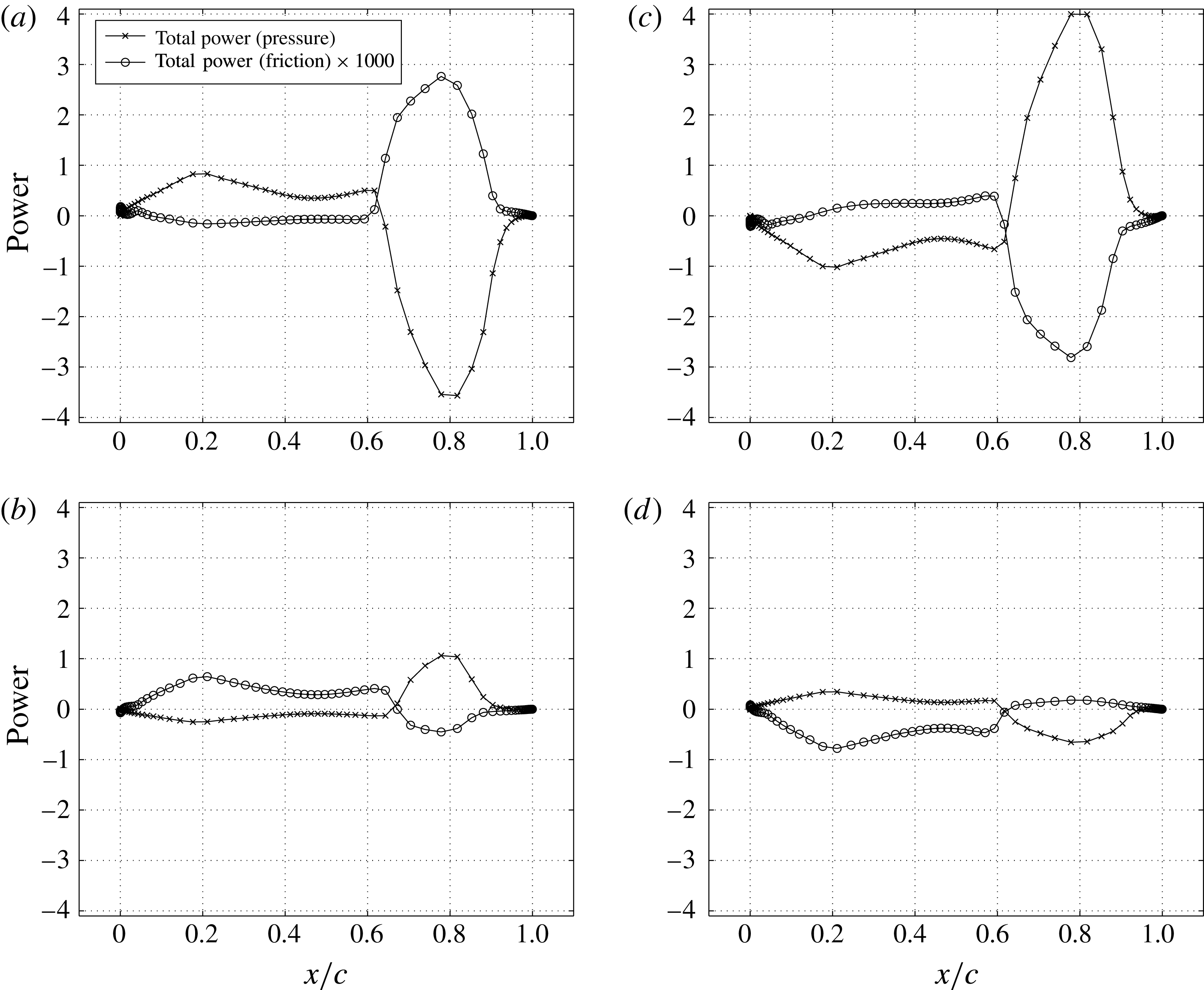
Now, rejoining the discussion on the viscous simulations, figure 16 shows the total power distribution on the airfoil camber line at different instants during a flutter cycle. In this case the airfoil oscillates about a new equilibrium position as the separated boundary layer keeps the nose of the airfoil down throughout. Since the distance between the two shocks, on the lower and upper surfaces of the airfoil, are large, the power transfer by the shock to the aeroelastic structure increases. It can be observed here too that the power due to viscous forces is almost three orders of magnitude lower than the pressure forces. But the important point to note here is that the interaction between the boundary layer and the shocks over the airfoil surface manipulates the power flow to the elastic system such that the observed flutter boundary and the dynamic characteristics of the aeroelastic system are drastically different from what is observed in the inviscid case.
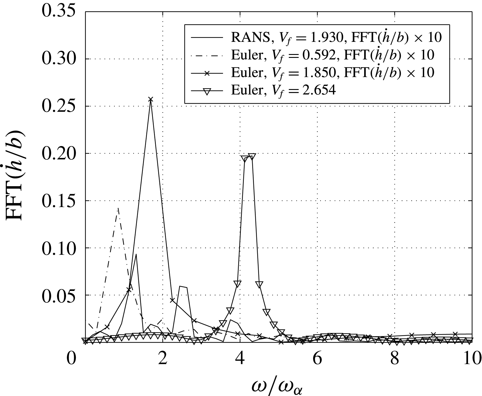
We also examined the frequency content of the response of the aeroelastic system as shown in figure 17. For this the Fourier transform of the heave velocity of the two degrees of freedom system is considered. We chose the velocity rather than the displacement to avoid the zero frequency response of the heave amplitude due to the shift in equilibrium position. The Fourier transform of the three inviscid flutter responses at this Mach number are also shown in this figure. It can be seen that the inviscid flutter response in each case has a single peak whereas the viscous fluid flow flutter response has three dominant peaks, decreasing in amplitude as their frequency increases. These three frequencies are:
 $\unicode[STIX]{x1D714}/\unicode[STIX]{x1D714}_{\unicode[STIX]{x1D6FC}}\approx 1.2,2.4,3.6$
. One also observed these frequency components in the flutter heave response in figure 7 earlier. The heave response clearly shows the periodic nature of the signal and the presence of harmonics. Fluid dynamic forces arising because of shock-induced separation is responsible for the multiple forcing frequencies of the aeroelastic system. Unlike in the inviscid simulation, viscous effects lead to separation of fluid that in turn lead to shock reversal (Bendiksen Reference Bendiksen2009), thereby increasing the number of aerodynamic forcing frequencies. Apart from these effects, the flow separates during some instants of the cycle and remains attached during other instants on the upper surface of the airfoil shown in figure 8. Therefore, multiple frequencies are present in the flutter response of the aeroelastic system caused by shock-induced separation and shock reversal in this region of the flutter boundary where viscous effects are significant.
Frequency content for
 $M_{\infty }=0.875$
flutter case.

5 Summary
Single mode flutter dominates in the lower Mach number interval of the transonic dip region: near
 $0.825$
. This suggests that the energy pumping mechanism here is the unsteady shock motion unlike in the case of classical bending-torsion flutter. This is also suggestive of the fact that viscosity has no significant influence in changing the behaviour of the system response in this Mach number range, as the same single mode response is observed even in the case of the inviscid transonic flutter boundary. Until this point in the flutter boundary, viscous and inviscid flutter points follow the same trend and are very close to one another with a slight shift towards the higher flutter index for the viscous case. Weakening of the shock strength due to viscous effects is responsible for this upward shift in the flutter index thereby mildly stabilizing the aeroelastic system. However, between
 $0.825<M_{\infty }<0.925$
, first an increase in Mach number increases the strength of the shock leading to separation. But the separated flow reattaches onto the airfoil surface. This effect of viscosity is reflected on the flutter boundary by a sudden jump in the flutter index. A drastic change in the flutter boundary is seen in the regime where the shock causes separation. Multiple frequencies are now seen in the aeroelastic response. At Mach numbers
 ${\geqslant}0.925$
, the shock strength increases and it shifts the shock towards the trailing edge thereby reducing the region of viscous influence to a small area near the trailing edge of the airfoil. Once again the viscous flutter boundary coincides with the inviscid flutter boundary.
The interval
 $0.825<M_{\infty }<0.925$
is the most affected by shock-induced boundary layer separation. The aerodynamic power due to pressure forces is three orders of magnitude greater than the power due to viscous forces acting on the airfoil surface alone. However, viscosity manipulates the strength and location of the shock and changes the magnitude and location of the resultant aerodynamic force acting on the elastic airfoil, leading to participation of two modes in the overall motion. In particular, at
 $M_{\infty }=0.875$
, these oscillations with two modes participating occurs about a new equilibrium point. Limitations of the Boussinesq turbulence models and the numerical methods adopted lead to quantitatively sensitive flutter boundary but they are qualitatively similar, especially in the Mach number range where shock-induced boundary layer separation is significant. Aeroelastic experiments, or an acceptable numerical model that can resolve turbulence, can validate these results.
The results presented in this work are for a particular instance of a two-dimensional aeroelastic system, and in general will vary as system parameters change. In a three-dimensional case, the flow structure will be a lot more complex, with features such as lambda shocks, along with other fluid–elastic features, that may influence the flutter boundary. However, these numerical simulations are pointers to the importance of viscosity and shock–boundary layer interactions, in unsteady transonic flows in general, and their influence on transonic flutter characteristics in particular.
Acknowledgement
The research presented here was partially supported by the Aeronautical Development Agency (ADA), India. We gratefully acknowledge their support.
Supplementary movies
Supplementary movies are available at https://doi.org/10.1017/jfm.2017.629.
Appendix A. Validation of the flow solver
The flow solver is validated first for flow over stationary airfoils and then flow over pitching airfoils. Structured grids of C-type are generated around the airfoil in all viscous flow simulations. C-type grids are represented by three numbers
 $n1\times n2\times An3$
with first number
 $n1$
representing the number of grids around the airfoil and cut lines, the second number
 $n2$
representing the number of grids normal to the surface of the airfoil and the third number
 $An3$
representing the number of grids on the airfoil surface. The far-field boundary is set at
 $20$
chord lengths away from the airfoil for all cases.
A.1 Stationary airfoil
In order to validate the flow solver, a grid convergence study was carried out for the flow over a stationary NACA 0012 airfoil held at an angle of attack of
 $1.77^{\circ }$
in a flow of Mach number
 $0.502$
and Reynolds number
 $2.91\times 10^{6}$
. The grids considered for the study are of size
 $256\times 72\times A160$
and
 $320\times 90\times A200$
. In both cases grid spacing normal to the solid surface is set equal to
 $8\times 10^{-6}$
times the chord length which corresponds to
 $y^{+}=1.0$
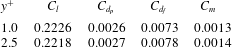
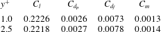
for the given Reynolds number. The aerodynamic coefficients computed using these grids are shown in table 1. It can be observed that grids of size
 $256\times 72\times A160$
can resolve the flow with considerable accuracy. A similar convergence study is performed by varying the grid spacing on the solid surface, that is for
 $y^{+}=1.0$
and
 $y^{+}=2.5$
. The aerodynamic coefficients computed are tabulated in table 2. The grid with
 $y^{+}=2.5$
has computed the aerodynamic coefficients with a maximum error of
 $8\,\%$
when compared with grids having
 $y^{+}=1.0$
. Throughout our computation grids of size
 $256\times 72\times A160$
with a
 $y^{+}=1.0$
are used.
Convergence study of NACA 0012 airfoil at
 $M_{\infty }=0.502$
,
 $Re_{\infty }=2.91\times 10^{6}$
at
 $\unicode[STIX]{x1D6FC}=1.77^{\circ }$
.

Convergence study of NACA 0012 airfoil at
 $M_{\infty }=0.502$
,
 $Re_{\infty }=2.91\times 10^{6}$
at
 $\unicode[STIX]{x1D6FC}=1.77^{\circ }$
with grids 256
 $\times$
72 with different normal grid spacing.
Turbulent flow computations were done on NACA 0012 and RAE 2822 airfoils which are held stationary at an angle to the flowing fluid. Experimental results are available for these cases for validation.
Validation of RANS solver for NACA 0012 airfoil;
 $M_{\infty }=0.502$
,
 $Re_{\infty }=2.91\times 10^{6}$
at
 $\unicode[STIX]{x1D6FC}=1.77^{\circ }$
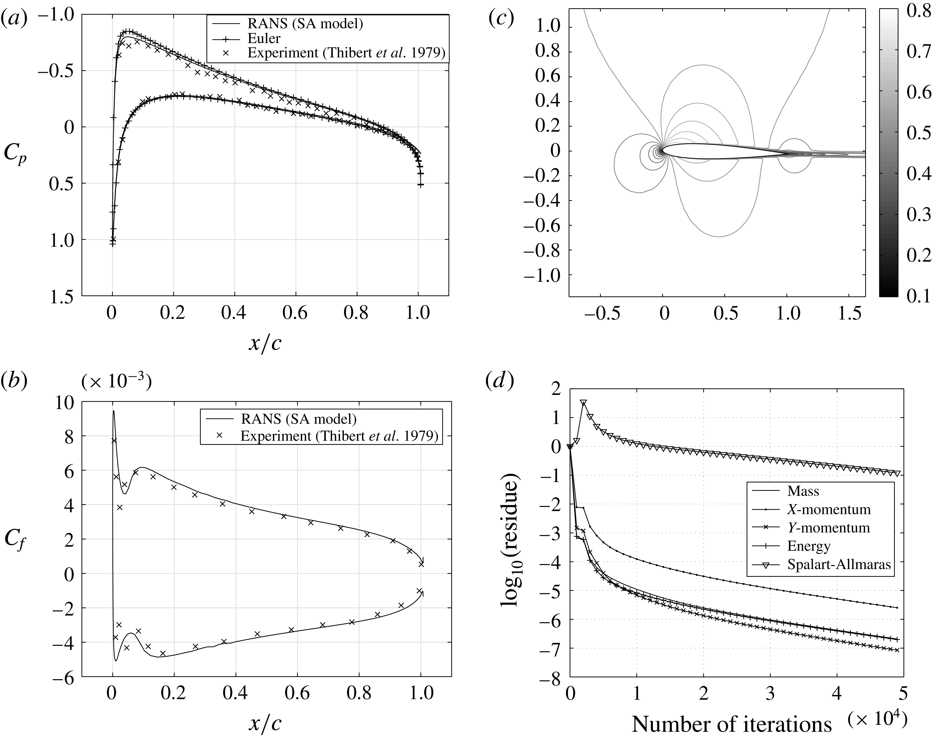
: (a) coefficient of pressure variation on the chord; (b) coefficient of friction variation on the chord; (c) mach contours over the airfoil; (d) residue decay with iterations.

Validation of RANS solver for RAE 2822 airfoil;
 $M_{\infty }=0.73$
,
 $Re_{\infty }=6.5\times 10^{6}$
at
 $\unicode[STIX]{x1D6FC}=2.79^{\circ }$
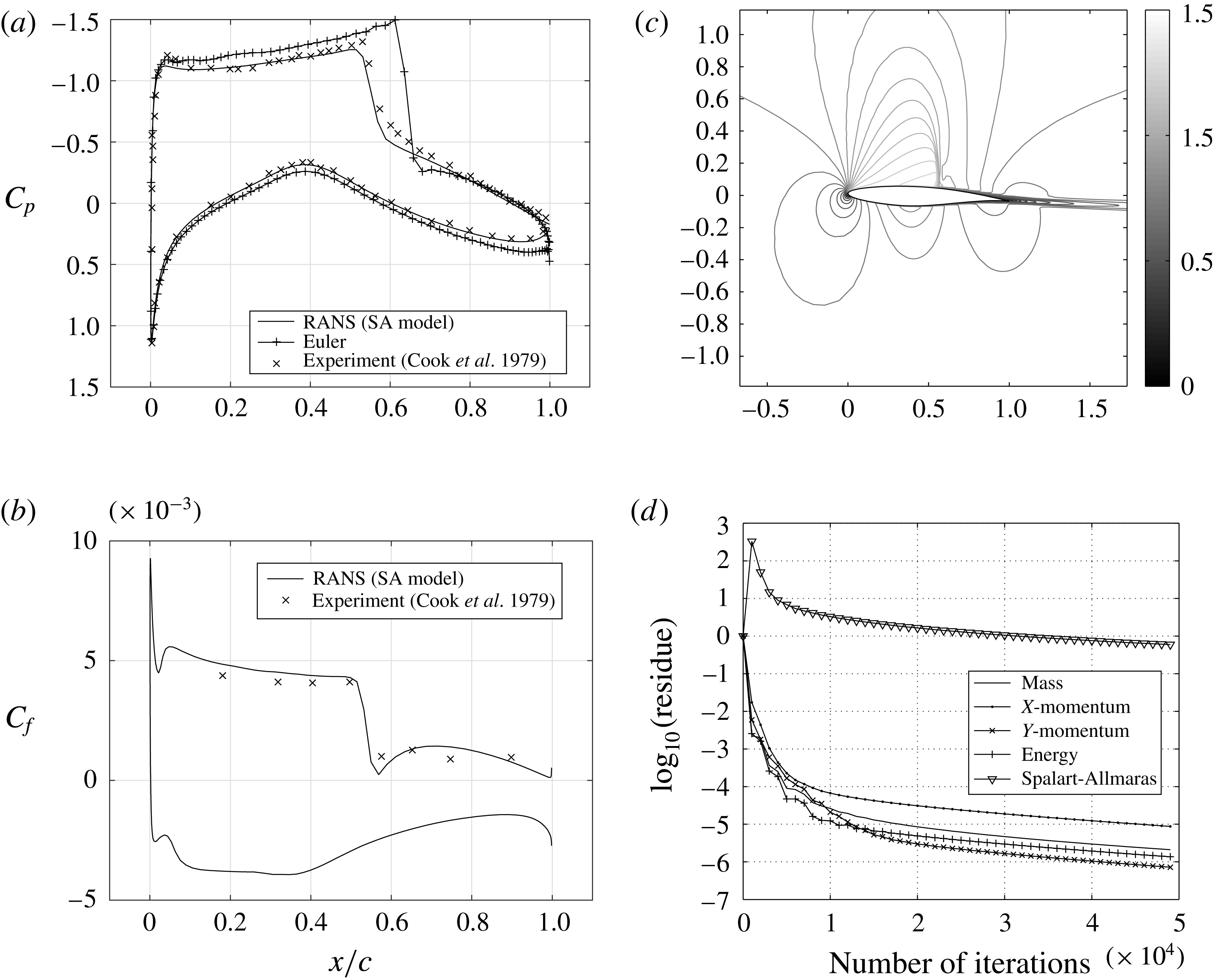
: (a) coefficient of pressure variation on the chord; (b) coefficient of friction variation on the chord; (c) mach contours over the airfoil; (d) residue decay with iterations.

A.2 NACA0012 airfoil
The first case considered is turbulent flow over NACA 0012 airfoil held at
 $1.77^{\circ }$
angle of attack in a flow of Mach number
 $0.502$
and Reynolds number
 $2.91\times 10^{6}$
(Thibert, Grandjacques & Ohman Reference Thibert, Grandjacques and Ohman1979). Figure 18 shows the coefficient of pressure distribution, coefficient of friction distribution, Mach contours and residue decay with iterations. The pressure distribution is shown in figure 18(a) and is compared with the experimental results of Thibert et al. (Reference Thibert, Grandjacques and Ohman1979). The numerical results are in close agreement with the experimental results. Inviscid results for the same case are superimposed over this figure which predicts the pressure distribution to a considerable accuracy. A small deviation near the lowest pressure point on the upper surface is observed for the inviscid case. The absence of viscous diffusion makes the fluid attain higher velocities than the viscous fluid and hence a deviation in pressure is seen around this point. Similarly at the trailing edge the pressure recovery for the inviscid case is higher compared to the viscous case. The skin friction distribution on the airfoil surface is shown in figure 18(b). The computed friction coefficient is compared with the experimental results which are superimposed in the same figure. From the skin-friction plot it can be concluded that the flow has not separated on the airfoil as the skin-friction coefficient curves do not cross the
 $C_{f}=0.0$
line. Figure 18(c) shows the iso-Mach lines for the flow considered. These Mach lines indicate that the complete flow field is subsonic in this case. Figure 18(d) shows the decay of residue with number of iterations. The residues dropped almost six decades for all governing equations except the turbulence model equation. This test case indicates that the inviscid computation is a good approximation for turbulent fluid flow simulation in subsonic flows at low angles of attack.
A.3 RAE2822 airfoil
The next case considered is the turbulent flow over RAE 2822 airfoil. Here the airfoil is held in a flow of Mach number
 $0.73$
, Reynolds number
 $6.5\times 10^{6}$
at an angle of
 $2.79^{\circ }$
to the free stream. Figure 19 shows the variations of coefficient of pressure, skin friction on the airfoil surface, Mach contour over the airfoil and residue decay with iterations. A sudden change in pressure distribution can be seen in figure 19(a) indicating the presence of shock on the airfoil surface. The local fluid velocity on the airfoil surface increases because of the airfoil geometry that can be seen in figure 19(c). This supersonic pocket ends with a shock shown by a sudden decrease in Mach number. Pressure and skin friction distributions are compared with the available experimental results of Cook, McDonald & Fermin (Reference Cook, McDonald and Fermin1979). The computed numerical viscous results are in close agreement with the experimental results. Shock strength and location are captured accurately. Inviscid numerical results are also superimposed over these results. Inviscid shock strength and location are far and away from either experimental or RANS solutions. This is because of the boundary layer, which changes the airfoil profile for the external flow field. As in the case of the NACA 0012 airfoil, the fluid has not separated anywhere on the airfoil, and can be seen in figure 19(b). Convergence in this case too is achieved with residues of each governing equation dropping by almost six decades except the turbulence model equation – shown in figure 19(d).
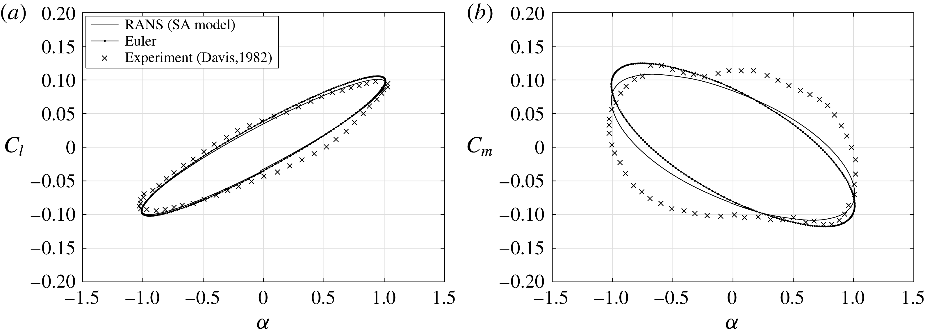
Lift and moment coefficient history for AGARD CT6 test case: (a) coefficient of lift versus angle of attack; (b) coefficient of moment versus angle of attack.

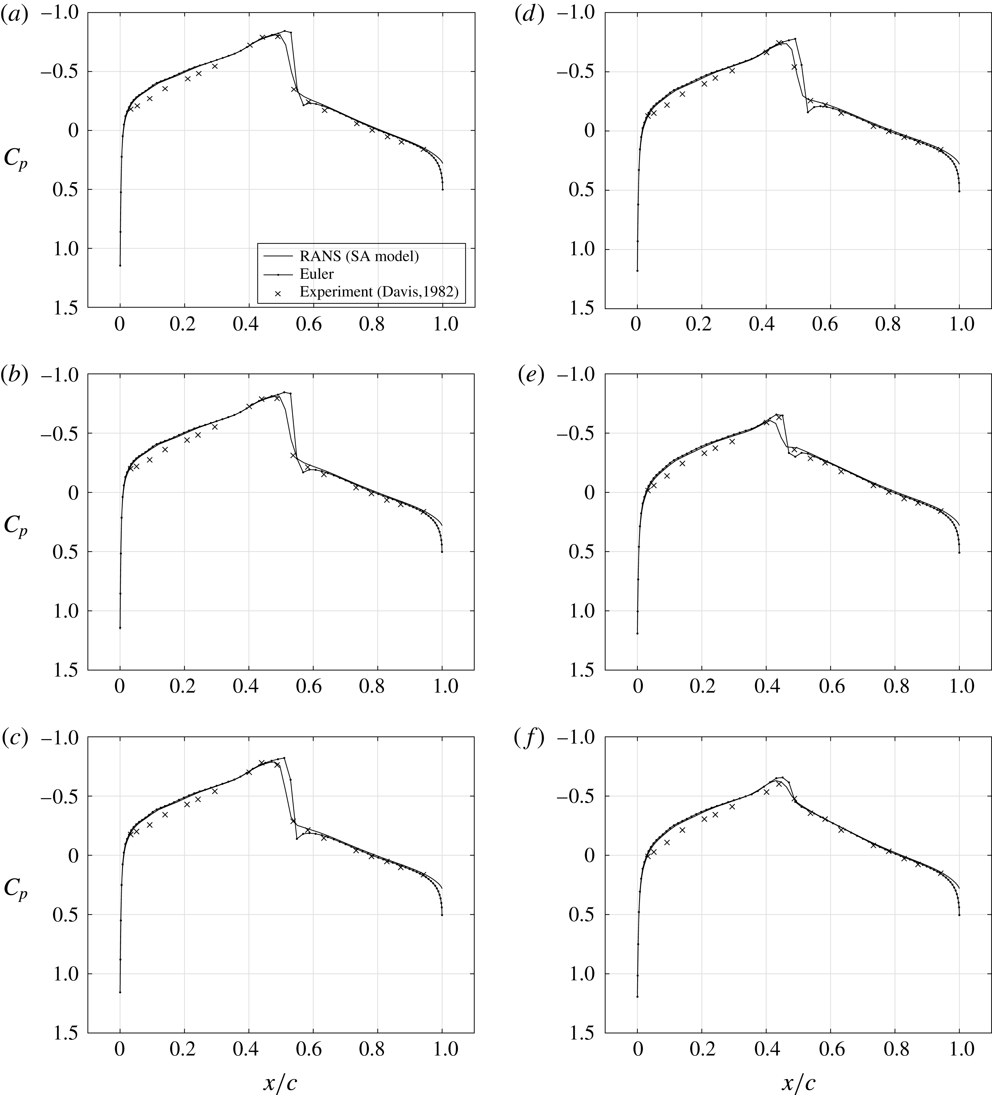
Instantaneous pressure distribution for AGARD CT6 test case on the airfoil upper surface: (a)
 $\unicode[STIX]{x1D6FC}=0.99^{\circ },\unicode[STIX]{x1D711}=101.25^{\circ }$
; (b)
 $\unicode[STIX]{x1D6FC}=0.57^{\circ },\unicode[STIX]{x1D711}=146.25^{\circ }$
; (c)
 $\unicode[STIX]{x1D6FC}=0.08^{\circ },\unicode[STIX]{x1D711}=174.37^{\circ }$
; (d)
 $\unicode[STIX]{x1D6FC}=-0.49^{\circ },\unicode[STIX]{x1D711}=209.53^{\circ }$
; (e)
 $\unicode[STIX]{x1D6FC}=-1.01^{\circ },\unicode[STIX]{x1D711}=269.99^{\circ }$
; (f)
 $\unicode[STIX]{x1D6FC}=-0.40^{\circ },\unicode[STIX]{x1D711}=336.09^{\circ }$
.

A.4 Pitching airfoil
In order to study flow over a moving airfoil, pitching motion is prescribed to the airfoil in a flow. The equation governing the airfoil motion is
 $$\begin{eqnarray}\unicode[STIX]{x1D6FC}=\unicode[STIX]{x1D6FC}_{m}+\unicode[STIX]{x1D6FC}_{0}\sin \unicode[STIX]{x1D714}t.\end{eqnarray}$$
 $\unicode[STIX]{x1D6FC}$
is the instantaneous angle of attack,
 $\unicode[STIX]{x1D6FC}_{m}$
is the mean angle of attack and
 $\unicode[STIX]{x1D6FC}_{0}$
is the amplitude of oscillation in pitch. The frequency of oscillation
 $\unicode[STIX]{x1D714}$
is defined by the reduced frequency
 $\unicode[STIX]{x1D705}$
as
 $$\begin{eqnarray}\unicode[STIX]{x1D705}={\displaystyle \frac{\unicode[STIX]{x1D714}b}{U_{\infty }}}.\end{eqnarray}$$
Here
 $b$
is the semi-chord and
 $U_{\infty }$
is the free-stream velocity of the fluid. Steady state solution is calculated over the stationary airfoil at its mean angle of attack. The airfoil is set in motion impulsively as defined by (A 1). Unsteady calculations are performed and the lift and moment variations are observed after the transients in the solution die down. All unsteady flow computations are performed using grids of C-type and of size
 $256\times 72\times A160$
. Grid spacing normal to the solid surface is set equal to
 $y^{+}=1.0$
.
A.4.1 AGARD CT6
The unsteady transonic test case considered for numerical verification is the AGARD CT6 of Davis (Reference Davis1982). Here a NACA 64A010 airfoil is forced in pitching about its quarter chord in a flow of Mach number
 $0.796$
and Reynolds number
 $12.56\times 10^{6}$
and at a mean angle of
 $0^{\circ }$
with an amplitude of oscillation of
 $1.01^{\circ }$
at a reduced frequency of
 $0.202$
. Lift and moment coefficients are shown in figure 20. Inviscid numerical results are also superimposed on these figures which shows a slight variation with RANS results. The reasons for both inviscid and viscous solutions to be in close agreement with the experimental results are because of high Reynolds number, low angle of attack and the airfoil being thin. As the Reynolds number increases, the boundary layer thickness decreases leading to approximately the same profile for the external flow field of viscous and inviscid simulations. The NACA 64A010 airfoil used in the AGARD CT6 case being thin has a higher critical Mach number. Therefore the effect of a higher Mach number leading to shock-induced viscous effects is reduced.
Pressure distribution on the airfoil surface at different instants for AGARD CT6 test case are shown in figure 21. Inviscid pressure distribution are also superimposed over these results along with the experimental results of Davis (Reference Davis1982). It can be seen that the shock location and strength captured by the RANS solver is close to that predicted by experiment, whereas the inviscid solver captures a stronger shock aft of the experimentally predicted shock location. The effect of viscosity in changing the strength and location of the shock when the airfoil is oscillating is clearly seen once again