1 Introduction
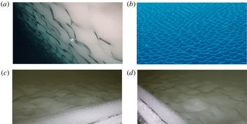
Interactions between a turbulent flow and an ablating surface material occur in a wide variety of contexts, often resulting in regularly spaced patterns of surface indentations known as scallops (see figure 1). These regular patterns, caused by differential ablation of the surface material, are ubiquitous in nature, having been observed in rock caves, sand, ice caves, river bedforms, snow, ice boreholes, inner walls of metal pipes, dissolvable bodies, icebergs, sea ice and river ice (e.g. Carey Reference Carey1966; Curl Reference Curl1966; Blumberg & Curl Reference Blumberg and Curl1974; Thomas Reference Thomas1979; Gilpin, Hirata & Cheng Reference Gilpin, Hirata and Cheng1980; Hanratty Reference Hanratty1981; Nelson, McLean & Wolfe Reference Nelson, McLean and Wolfe1993; Wykes et al. Reference Wykes, Mac Huang, Hajjar and Ristroph2018). These scallop examples encompass different fluids, materials and ablation mechanisms, namely, melting, erosion, dissolution and sediment transport. The unifying feature across this diverse set of examples is thought to be the fluid dynamics of turbulent flow adjacent to an erodible surface, and the corresponding ablation rates induced by this flow.
Photos of scallop formations on the sides of icebergs (a,b) and from the laboratory experiments of this study (c,d). Photos (a) and (b) were taken in the Southern Ocean with a remotely operated vehicle (Hobson, Sherman & McGill Reference Hobson, Sherman and McGill2011). Images courtesy of Brett Hobson, © 2009 Monterey Bay Aquarium Research Institute. Images (c) and (d) are courtesy of Denise Holland. The peak-to-peak wavelengths of these scallops (a–d) are roughly 10 cm, 10 cm, 12 cm and 12 cm, respectively.

A number of studies have examined the flow mechanisms responsible for the formation of scallops. In a pioneering work, Curl (Reference Curl1966) investigated limestone–water and ice–air scallop patterns in caves, observing that scallops tend to have a universal profile oriented along the direction of flow, with steeper slopes on their leeward sides than their streamward sides. Curl (Reference Curl1966) proposed that scallops satisfy a universally constant Reynolds number
 $Re^{\ast }=U\unicode[STIX]{x1D706}/\unicode[STIX]{x1D708}\approx 22\,500$
, where
 $U$
is the free-stream velocity,
 $\unicode[STIX]{x1D706}$
is the scallop wavelength and
 $\unicode[STIX]{x1D708}$
is the kinematic viscosity of the fluid. He suggested that this relationship could be used to deduce past flow speeds and directions from cave scallop patterns. Curl (Reference Curl1966) also noted that scallop patterns tend to propagate downstream in the direction of the flow, due to higher ablation rates on their streamward sides than their leeward sides.
Blumberg & Curl (Reference Blumberg and Curl1974) detailed a flow-driven mechanism for scallop formation, in which scallops form due to a self-reinforcing interaction between the geometry of the surface, the adjacent flow field and the resulting differential ablation rates that occur. Their proposed mechanism, motivated by dye tracer experiments, involved boundary-layer flow separation occurring at the scallop crest and a transition to turbulence of the separated flow, creating recirculating eddies in the scallop trough. Downstream of the recirculation zone, a reattachment of the flow occurs, and the flow pattern repeats as it travels over the subsequent scallop crest. This reattachment location corresponds roughly to the region of maximum ablation rates. In this work, the authors additionally suggested that a ‘scallop Reynolds number’ based on the friction velocity
 $u_{\ast }$
is more appropriate, and proposed a value of
 $Re^{\ast }=u_{\ast }\unicode[STIX]{x1D706}/\unicode[STIX]{x1D708}=2200$
.
Thomas (Reference Thomas1979) investigated the scalloping phenomenon across a remarkable range of materials and flow conditions. Using experimental data encompassing scallop wavelengths ranging from
 $50~\unicode[STIX]{x03BC}\text{m}$
to 1 m, he found an approximate relationship of
 $Re^{\ast }=u_{\ast }\unicode[STIX]{x1D706}/\unicode[STIX]{x1D708}=1000$
. Thomas (Reference Thomas1979) found that most data points satisfied this relationship within a factor of 2 or 3, supporting a ‘wall similarity hypothesis’ for scallop formation, in which the characteristic scallop wavelength is a universal multiple of the viscous sublayer length scale
 $\unicode[STIX]{x1D708}/u_{\ast }$
.
The focus of this work is scallops that form at the ice–water interface. Ice scallops typically occupy a parameter space spanning wavelengths of 5–20 cm and free-stream velocities of 0.10–1.50 m s
 $^{-1}$
. The ice–water interface evolution problem is a Stefan problem (Stefan Reference Stefan1891), involving a time-evolving boundary condition governed by phase changes between water and ice. Ice scallops occur in a regime in which the fluid flow is turbulent, resulting in a complex coupled interaction between the evolving ice geometry and the ice–water boundary layer (Gilpin et al.
Reference Gilpin, Hirata and Cheng1980). In laboratory experiments using fresh water, Ashton (Reference Ashton1972), Ashton & Kennedy (Reference Ashton and Kennedy1972), Hsu, Locher & Kennedy (Reference Hsu, Locher and Kennedy1979) and Gilpin et al. (Reference Gilpin, Hirata and Cheng1980) found that, under turbulent flow conditions, ice–water ripple patterns developed in response to an initial perturbation in the ice interface. They found that these ripple patterns deepened and migrated in the downstream flow direction over time, indicating that maximum heat transfer occurs downstream of the trough position. The ripple patterns in these studies were ‘two-dimensional’ with all crests aligned transverse to the flow direction. This geometry is distinct from ice scallops, which have a clear three-dimensional (3-D) structure resembling a hexagonal packing arrangement when viewed from above (see figure 1). Two-dimensional (2-D) ice ripples have been observed primarily in controlled settings with unidirectional flow, whereas 3-D scallop patterns are more commonly observed in nature (Gilpin et al.
Reference Gilpin, Hirata and Cheng1980). In their laboratory experiments, Gilpin et al. (Reference Gilpin, Hirata and Cheng1980) found that ice interfaces that developed 2-D ripples would eventually transition to 3-D scallop patterns.
Theoretical analyses have also provided insight into ice–water interface instabilities. Performing a 2-D linear stability analysis on a theoretical model of melting in the presence of a turbulent flow, Thorsness & Hanratty (Reference Thorsness and Hanratty1979a
) and Hanratty (Reference Hanratty1981) identified a range of unstable wavelengths for a melting surface, reporting positive growth rates for
 $2000\unicode[STIX]{x1D708}/u_{\ast }<\unicode[STIX]{x1D706}<18\,000\unicode[STIX]{x1D708}/u_{\ast }$
, with the most unstable wavelengths occurring in the range
 $3100\unicode[STIX]{x1D708}/u_{\ast }<\unicode[STIX]{x1D706}<6300\unicode[STIX]{x1D708}/u_{\ast }$
. These results agreed well with the experimentally derived relationship of
 $\unicode[STIX]{x1D706}=3180\unicode[STIX]{x1D708}/u_{\ast }$
of Hsu et al. (Reference Hsu, Locher and Kennedy1979). In recent work, Claudin, Durán & Andreotti (Reference Claudin, Durán and Andreotti2017) built upon the 2-D framework of Hanratty (Reference Hanratty1981) by explicitly incorporating the effects of surface roughness. Claudin et al. (Reference Claudin, Durán and Andreotti2017) provide predictions for the most unstable wavelengths and amplitudes, finding that unstable growth ceases when the surface became sufficiently rough, thereby suggesting a mechanism for the selection of the ripple amplitude. Interestingly, the linear stability analysis of Camporeale & Ridolfi (Reference Camporeale and Ridolfi2012) for 3-D laminar flows with a free surface revealed that interfacial instabilities can also occur in the laminar regime due to free surface effects.
In laboratory experiments, field observations and theoretical computations, scallops have been shown to increase turbulent heat transfer to the ice–water interface (Gilpin et al. Reference Gilpin, Hirata and Cheng1980; Seki, Fukusako & Younan Reference Seki, Fukusako and Younan1984; Wettlaufer Reference Wettlaufer1991; Feltham, Worster & Wettlaufer Reference Feltham, Worster and Wettlaufer2002), suggesting that they may have an important influence on overall melt rates of sea ice, icebergs and ice shelves. Small-scale turbulent heat transfer in the ice–ocean boundary layer has a profound impact on ice melt rates, yet these processes occur at scales well below those currently resolvable by general circulation models (GCMs) or regional ice–ocean models. In order to account for these crucial yet unresolvable processes, parametrizations must be used which utilize bulk information to estimate oceanic turbulent heat flux (Mellor, McPhee & Steele Reference Mellor, McPhee and Steele1986; McPhee, Maykut & Morison Reference McPhee, Maykut and Morison1987; Hellmer & Olbers Reference Hellmer and Olbers1989; Steele, Mellor & McPhee Reference Steele, Mellor and McPhee1989; Jenkins Reference Jenkins1991; McPhee Reference McPhee1992, Reference McPhee2008; Holland & Jenkins Reference Holland and Jenkins1999; Dansereau, Heimbach & Losch Reference Dansereau, Heimbach and Losch2014; Ramudu et al. Reference Ramudu, Hirsh, Olson and Gnanadesikan2016). A typical assumption of these parametrizations is that the ice interface is hydraulically smooth (Kader & Yaglom Reference Kader and Yaglom1972), thereby ignoring the potentially important effects of ice geometry on melt rates. Given the ubiquity of ice scallops in nature, it is crucial to investigate ice–water boundary-layer turbulence in the presence of complex ice geometries in order to guide future development of melt-rate parametrizations for use in large-scale numerical models.
While the studies above have demonstrated the crucial importance of the turbulent flow field in determining scallop formation and evolution, direct measurements of the turbulent boundary layer adjacent to an evolving ice–water interface have remained elusive, due to the small spatial scales and high-frequency fluctuations that characterize these flows. In this work, we explore scallops using recent experimental techniques, presenting direct observations of an evolving ice–water interface at sub-millimetre spatial resolution and 15 Hz temporal resolution. These data were obtained from a series of laboratory experiments performed in a refrigerated flume at the Cold Regions Research and Engineering Laboratory (CRREL). In these experiments, water of a specified free-stream velocity was flowed overtop a bed of initially flat freshwater ice and the subsequent ice geometry and flow changes were examined using flow measurements based on particle image velocimetry (PIV; Willert & Gharib Reference Willert and Gharib1991; Adrian Reference Adrian2005; Adrian & Westerweel Reference Adrian and Westerweel2011). These high-resolution data of the ice–water interface provide new insights into the flow-driven mechanisms underlying scallop formation and evolution.
The plan of this paper is as follows. In § 2, we describe the experimental set-up and measurement techniques used in the laboratory flume experiments. Section 3 investigates the evolution of the ice–water interface, identifying three distinct regimes of interface evolution. In § 4, we analyse flow measurements in the ice–water boundary layer, providing a detailed comparison of flow over flat and scalloped ice and proposing a mechanism for scallop formation involving a positive feedback between the ice-interface geometry and shear production of turbulent kinetic energy in the flow interior. In § 5, we present turbulent heat flux measurements collected near a scalloped interface. Section 6 considers these results in the context of melt-rate parametrizations used in numerical ice–ocean models. We present conclusions and future directions in § 7.
2 Experimental set-up and methods
2.1 Experimental set-up
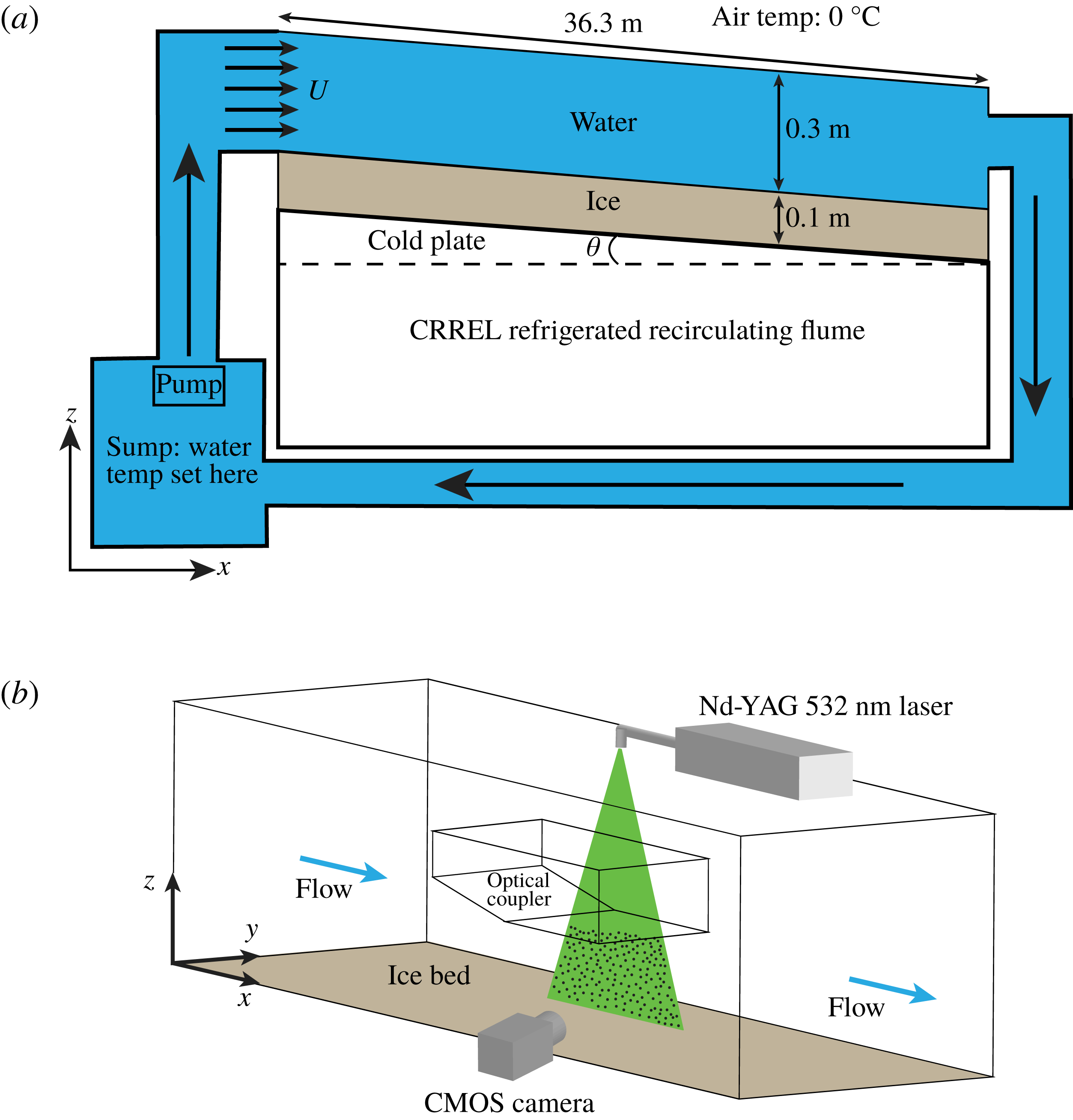
Experiments were performed in the CRREL recirculating flume (Richmond & Lunardini Reference Richmond and Lunardini1990), as depicted in figure 2. The flume is 36.6 m long, 1.2 m wide and 0.9 m deep, and is contained in a refrigerated room with air temperatures maintained at
 $0\,^{\circ }$
C. This air temperature is chosen to ensure that essentially all ice melting in these experiments occurs due to heat transfer between water and ice. Water is pumped into the flume at a specified volume flux, which ranges from 0 to 0.38 m
 $^{3}$
s
 $^{-1}$
, and recirculates in a closed loop. The flume system has a total water capacity of 169 m
 $^{3}$
. When not flowing through the system, the water is stored in a sump, where its temperature is controlled via heating and cooling coils. Additionally, the flume is capable of being tilted up to
 $1.1^{\circ }$
relative to the horizontal. The volume flux and flume tilt are the main parameters that control the free-stream velocity. Typical flow depths in these experiments were roughly 0.3 m, and all experiments were performed using fresh water. The CRREL flume has an open top and glass sides, which provide easy physical and optical access to the measurement region of interest near the ice–water interface. Also, the flume sides are equipped with rails and a sliding carriage, which allows for quick movement of the measurement apparatus to different sections of the flume.
Experimental set-up in the CRREL refrigerated recirculating flume. Panel (a) shows the movement of water through the system, and (b) shows the set-up of the measurement region.

The flume bed is equipped with a refrigerated plate, which can be held at a fixed temperature between
 $-29\,^{\circ }$
C and
 $10\,^{\circ }$
C, with a precision of
 $0.3\,^{\circ }$
C. For each experiment, a flat 10–15 cm thick sheet of freshwater ice was grown overnight on top of the flume bed. A specified free-stream velocity, water temperature and cold-plate temperature were chosen for each experiment, and water with these properties was flowed overtop of ice that was initially flat relative to the flume bed. The water temperature was measured using a thermistor with an error level of
 $0.1\,^{\circ }$
C. The free-stream velocity was initially chosen based on the water volume flux and flow depth, and subsequently was measured using PIV (see below), which has an error level of roughly 0.01 m s
 $^{-1}$
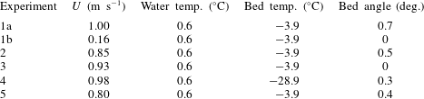
. A number of experiments were performed exploring this parameter space, and we primarily focus on a subset of these experiments (see table 1). A full table of the experiments performed is provided in the supplementary material available at https://doi.org/10.1017/jfm.2019.398. It should be noted that for some initial experiments, semi-cylindrical perturbations in the ice surface were created by placing PVC pipes into the ice as it froze. These perturbations were inspired by the findings of Gilpin et al. (Reference Gilpin, Hirata and Cheng1980), but we found that perturbations were not necessary to create scallop patterns and this technique was abandoned. All results in this paper are based on ice that was initially flat with millimetre-scale imperfections.
Summary of the experiments presented in this study.

2.2 Particle image velocimetry data
Quantitative flow measurements of the velocity field near the ice–water interface are made using 2-D PIV (Willert & Gharib Reference Willert and Gharib1991; Adrian Reference Adrian2005; Adrian & Westerweel Reference Adrian and Westerweel2011). The experimental set-up of the test region is shown in figure 2(b). This set-up is designed to capture two images of illuminated tracer particles in the fluid in quick succession, allowing for a velocity field to be computed by performing a cross-correlation analysis on the images. The fluid is seeded using 10
 $\unicode[STIX]{x03BC}$
m diameter glass beads, which are nearly neutrally buoyant in fresh water and are advected by the flow as nearly passive tracers.
A double-pulsed 532 nm Nd:YAG laser is placed on the flume’s sliding carriage at a fixed
 $y$
-position (see figure 2
b). The laser produces a well-collimated beam of light which passes through a cylindrical lens that produces a thin (0.5 mm) sheet of laser light in the
 $x{-}z$
plane. The glass beads effectively scatter the laser light, illuminating the tracer particles. A scientific complementary metal oxide semiconductor (sCMOS) camera with
 $2560\times 2160$
pixel resolution, 16 bits per pixel dynamic range, a 105 mm lens and
 $f$
-stop value of 2.8 is placed outside the flume and directed perpendicular to the
 $x{-}z$
plane. Some data were also collected using a 60 mm lens, which provided a larger field of view. The camera and laser are synchronized using a programmable timing unit such that the camera captures two images in rapid succession corresponding to the double pulse of laser light. For these experiments, the gap between laser pulses was
 $\unicode[STIX]{x0394}t=1~\text{ms}$
, and these double pulses fired at a frequency of 15 Hz (67 ms period). The camera was positioned at a
 $z$
-location chosen to capture the ice–water interface and the water above it. A typical field of view was roughly 6 cm
 $\times$
6 cm. As the ice melted over the course of the experiment, the camera was intermittently moved down in order to keep the ice–water interface in the camera’s field of view. For each
 $y$
-position of the laser, a calibration step was performed by recording images of a calibration plate that has a matrix of dots with known spacings and is placed in the
 $x{-}z$
laser plane. The camera was fitted with a bandpass filter at 532 nm
 $\pm$
10 nm to limit ambient background light from the images.
An experimental challenge was the refraction of laser light due to waves on the free upper surface of the water. In order to remedy this, an ‘optical coupler’ was constructed to allow for a rigid lid surface condition above the PIV study region. The optical coupler is a 2 m
 $\times$
1 m
 $\times$
0.3 m rectangular tub with a shallow ramp along its leading edge and a Plexiglas bottom above the study region (see figure 2
b). The optical coupler was lowered roughly 2 cm into the water in order to produce minimal flow disturbance while providing a flat optical surface for the laser sheet to be transmitted into the body of flowing water. The qualitative melt features observed underneath the optical coupler are indistinguishable from other portions of the flume, indicating that the coupler had no discernible influence on turbulent heat fluxes at the ice–water interface.
Data acquisition of PIV images was limited by the speed at which data could be written to disk. The typical data acquisition period was 6.7 s (100 double images), and one of these datasets was captured roughly every 120 s. The collected PIV images are analysed using commercial PIV software (DaVis 8.0 by LaVision). Velocity vectors are obtained using a multi-pass cross-correlation procedure which begins with 64
 $\times$
64 pixel PIV interrogation regions with 50 % overlap, and concludes with 32
 $\times$
32 pixel PIV interrogation regions. For consistency, we apply the same processing algorithm across all images and all experiments. No smoothing is applied to the output velocity vectors and no masking of the image is applied. Uncertainty quantification of the velocity vectors is performed using a correlation peak statistics algorithm (Wieneke Reference Wieneke2015), which shows that errors of the instantaneous velocities typically range from 2 % to 10 % of the velocity magnitude and tend to be larger in regions of enhanced velocity gradients. These errors are reduced under time averaging, yielding typical time-mean velocity errors of less than 1 %. The errors in time-mean velocity gradients are substantially larger when considered at a grid-point scale, ranging from 10 % to 60 % of the background shear values; however, the spatial coherence of velocity gradients over larger spatial scales increases our confidence in the computed values.
2.3 Heat flux measurements
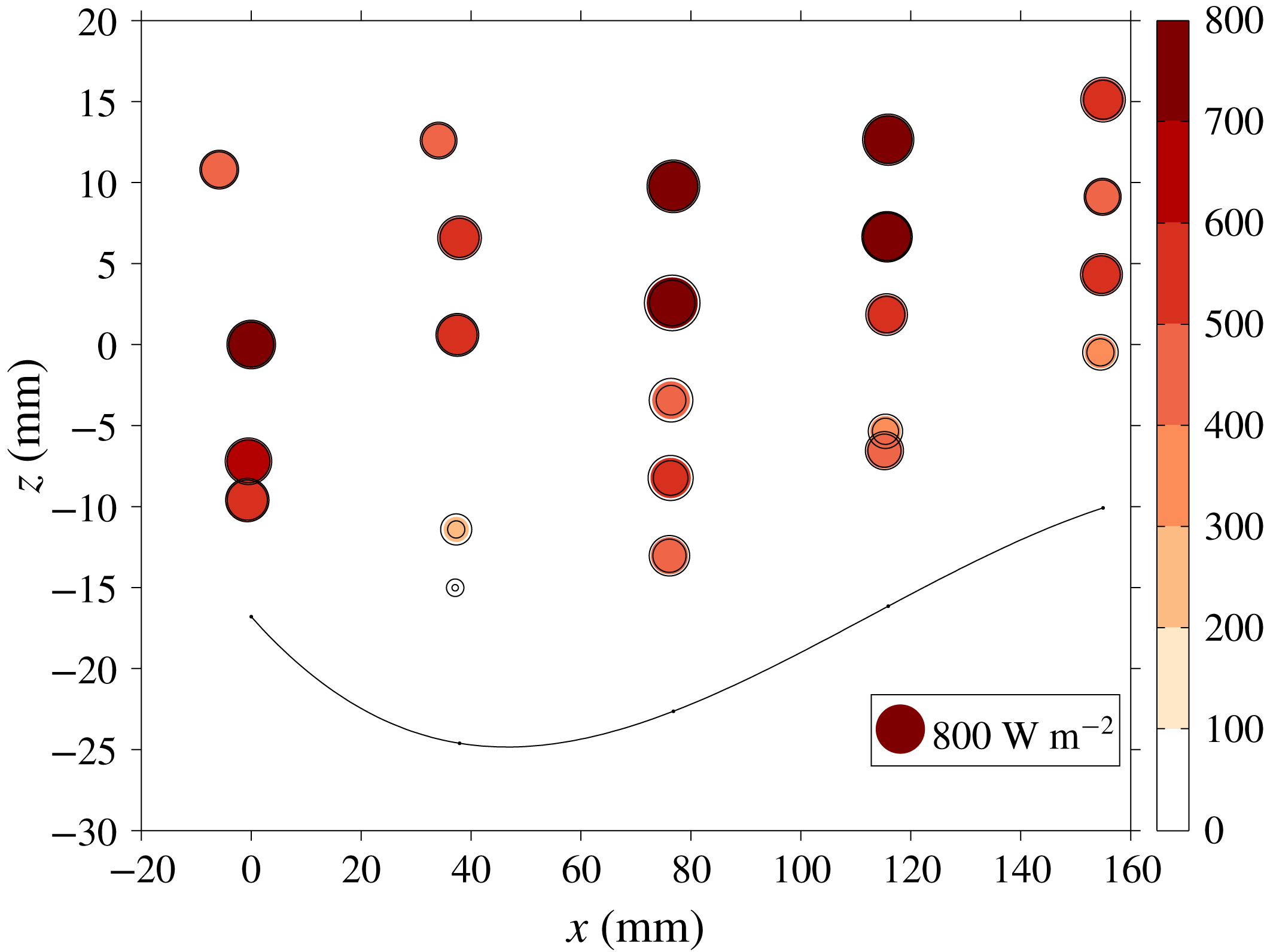
For experiment 5, a series of heat flux measurements were made in the trough region of a well-developed scallop by collecting simultaneous and nearly spatially coincident measurements of temperature and vertical velocity. Velocity measurements were collected using a 5 MHz bistatic coherent Doppler velocity profiler (BCDV; Stanton Reference Stanton2001) and temperatures were collected using an FP07 fast microthermistor (Goto, Yasuda & Nagasawa Reference Goto, Yasuda and Nagasawa2016) sampling at 200 Hz. The BCDV and thermistor have root-mean-square (r.m.s.) noise levels of 0.004 m s
 $^{-1}$
and 0.001 K, respectively. The BCDV was placed at a given
 $x$
-position and provided vertical velocity measurements in 1.2 mm bins. The thermistor was placed immediately downstream (roughly 1 mm) of the BCDV measurement region, allowing for collocated and simultaneous measurements of the vertical velocity
 $w$
and temperature
 $T$
and computation of the turbulent heat flux
 $w^{\prime }T^{\prime }$
, where the prime symbol indicates deviations from the time mean. By sampling different
 $z$
-positions with the thermistor and moving the BCDV to different
 $x$
-positions within the scallop trough, we are able to ‘resolve’ the vertical turbulent heat fluxes within a scallop trough. At each
 $(x,z)$
position,
 $w$
and
 $T$
are sampled for 1 min in order to obtain robust eddy statistics. The standard deviation of the measured vertical heat flux
 $w^{\prime }T^{\prime }$
was estimated by a bootstrap method (Emery & Thomson Reference Emery and Thomson2001) in which the 1 min time series were randomly subsampled in 15 s sections, the
 $w^{\prime }T^{\prime }$
covariance estimated for each subsection, and the mean and standard deviation of the resulting sample set calculated. In addition to temporal sampling error, there is potential for systematic heat flux errors associated with the 1 mm gap between the BCDV and thermistor measurements. We expect these errors to be small, as the 1 mm spacing between these measurements is small compared to the typical length scale of velocity fluctuations in this flow. For each measurement, the height above the ice–water interface was determined using the BCDV backscatter profile, and the position relative to a Lagrangian reference point at the scallop crest was determined using a measured downstream scallop advection velocity of 0.11 mm min
 $^{-1}$
.
2.4 Ice–water interface identification
A key element of this study is the identification of the ice–water interface using PIV images. After testing a number of approaches, we found that the interface could be robustly identified using the temporal variance of the PIV-derived velocity fields. In particular, the ice–water interface stands out as a thin low-variance strip when the velocity variance is plotted. To identify the interface, for each
 $x$
we search vertically downwards and find the first
 $z$
-value that falls below a specified threshold. These interface estimates have errors of roughly 1 mm and also contain occasional outliers. After this, the interface estimates are smoothed using MATLAB’s robust locally weighted linear regression function with a filtering span of 20 % of the domain length, yielding a final interface
 $z=h(x)$
. This technique was found to work well even with low-quality PIV data, meaning it could be applied to data across all of our experiments. Melt rates computed from these interface profiles have errors that depend on the time-averaging period. Typical melt-rate errors for the results presented in this paper range from 0.03 to 0.06 mm min
 $^{-1}$
.
2.5 Experimental challenges and limitations
A number of experimental challenges were encountered in attempting to capture high-resolution velocity data at the ice–water interface using PIV. A first challenge was a tradeoff related to laser intensity. High laser intensities are preferable, as they provide maximal illumination of the PIV particles; however, when using high intensities we encountered significant reflections from the ice surface, which saturated the boundary-layer portion of the image. Achieving an unsaturated image is necessary to allow background subtraction of the bright laser line on the ice surface, which then reveals particles near the ice–water boundary. Subtracting this background image prevents this laser line from dominating the cross-correlation and allows for detection of the particle displacement correlation peak, thus resolving velocity vectors close to the ice surface. Therefore, these laser reflections necessitated the use of lower laser intensities, which generally degraded the image quality and subsequent PIV-derived vector fields. A potential solution to this is the use of fluorescent PIV particles, which emit at a different wavelength than the Nd:YAG laser. By using a bandpass filter, the reflected laser light can be filtered out, allowing for the fluorescent particles to be captured using high laser intensities. We experimented with this approach, fabricating fluorescent particles following the methodology of Pedocchi, Martin & García (Reference Pedocchi, Martin and García2008), and had encouraging preliminary results. Unfortunately, the difficulty of fabricating a large mass of fluorescent particles precluded their use across our experiments.
Another challenge was the tradeoff between the camera field of view and the quality of the PIV-derived velocity vectors. We initially collected data using a roughly 150 mm
 $\times$
150 mm field of view, which provided data over a region spanning 1–2 scallop wavelengths. With a field of view of this size, the scallop trough occupies a small fraction of the image, and the PIV-derived velocity vectors did not have sufficient spatial resolution for a detailed analysis of turbulence in this region. It was found that using a smaller field of view of roughly 60 mm
 $\times$
60 mm yielded substantially higher-quality data with good resolution of the scallop trough region. The downside to this smaller field of view is that most of our data only capture a portion of a scallop wavelength, and this does not allow us to directly observe periodic flow structures.
As mentioned in § 2.1, having an optical coupler that allowed the laser to pass through a consistent upper water surface while creating minimal flow disturbance was essential. Data collected without the optical coupler were of extremely poor quality due to deflection of the laser sheet. We also note that the laser sheet was positioned at
 $y$
-locations corresponding to the middle of scallop troughs to limit out-of-plane reflections of the laser sheet. Finally, we also experimented with stereo PIV, which uses two cameras and allows out-of-plane velocities to be inferred. In general, we found that the stereo PIV data were of lower quality than the 2-D PIV data, due to astigmatism from viewing into the flume at an oblique angle to the glass sidewall. Because of this, we focused most of our efforts on obtaining high-quality 2-D PIV data in the
 $x{-}z$
plane. Given the observed 3-D geometry of scallops, with notable height variations occurring in both the along-flow and out-of-plane directions (see figure 1), future experiments targeted at measuring the 3-D velocity structure within a scallop are required.
3 Ice–water boundary evolution
3.1 Problem set-up
The ice–water boundary evolution problem is a fluid–structure interaction, commonly referred to as the Stefan problem (Stefan Reference Stefan1891). This problem involves a coupled interaction between water and ice, in which the turbulent flow field and corresponding heat transfer melts or freezes ice and modifies the geometry of the ice–water interface, thereby feeding back on the flow. We analyse our laboratory results using the following set of coupled partial differential equations to describe the ice–water interaction. The water portion of the domain is governed by the homogeneous, incompressible, non-hydrostatic 2-D (
 $x,z$
) Navier–Stokes equations:
 $$\begin{eqnarray}\displaystyle \unicode[STIX]{x1D70C}{\displaystyle \frac{\unicode[STIX]{x2202}\boldsymbol{u}}{\unicode[STIX]{x2202}t}}+\unicode[STIX]{x1D70C}\boldsymbol{u}\boldsymbol{\cdot }\unicode[STIX]{x1D735}\boldsymbol{u}=-\unicode[STIX]{x1D735}p+\unicode[STIX]{x1D707}\unicode[STIX]{x1D6FB}^{2}\boldsymbol{u}-\unicode[STIX]{x1D70C}g\hat{\boldsymbol{k}},\quad \unicode[STIX]{x1D735}\boldsymbol{\cdot }\boldsymbol{u}=0,\quad \unicode[STIX]{x1D70C}=\unicode[STIX]{x1D70C}_{w}, & & \displaystyle\end{eqnarray}$$
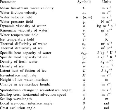
where these symbols are defined in table 2. Given that all experiments were performed with fresh water and over a small temperature range (in nearly all experiments the water was between 0
 $^{\circ }$
C and 1
 $^{\circ }$
C), we choose to model the water as a constant-density fluid. A scaling argument using a typical velocity and length scale for ice scallops shows that the buoyancy term,
 $g\unicode[STIX]{x0394}\unicode[STIX]{x1D70C}$
, is
 ${<}10^{-3}$
times the size of the advective term in the momentum equation. Therefore, we have neglected the buoyancy term in (3.1), treating the fluid as having constant density. Note that in oceanographic contexts with salt water adjacent to icebergs or sea ice, the buoyancy term will likely be an important contributor to the momentum budget and the scallop formation mechanism. We also note that out-of-plane velocity fluctuations are likely to play an important role in setting the 3-D structure of ice scallops, but were not measured with our 2-D PIV laboratory set-up.
Symbols used in this study.

The temperature evolution in the water portion of the domain is governed by an advection–diffusion equation,
 $$\begin{eqnarray}\displaystyle {\displaystyle \frac{\unicode[STIX]{x2202}T_{w}}{\unicode[STIX]{x2202}t}}+\boldsymbol{u}\boldsymbol{\cdot }\unicode[STIX]{x1D735}T_{w}=\unicode[STIX]{x1D735}\boldsymbol{\cdot }(\unicode[STIX]{x1D705}_{w}\unicode[STIX]{x1D735}T_{w}), & & \displaystyle\end{eqnarray}$$
and the ice temperatures satisfy a diffusion equation,
 $$\begin{eqnarray}\displaystyle {\displaystyle \frac{\unicode[STIX]{x2202}T_{i}}{\unicode[STIX]{x2202}t}}=\unicode[STIX]{x1D735}\boldsymbol{\cdot }(\unicode[STIX]{x1D705}_{i}\unicode[STIX]{x1D735}T_{i}). & & \displaystyle\end{eqnarray}$$
Finally, the melting/freezing of ice is governed by an interface condition, which enforces the conservation of heat across the ice–water interface:
 $$\begin{eqnarray}\displaystyle Q_{w}-Q_{i}=\unicode[STIX]{x1D70C}_{w}c_{p,w}\unicode[STIX]{x1D705}_{w}\unicode[STIX]{x1D735}T_{w}\boldsymbol{\cdot }\hat{\boldsymbol{n}}|_{b}-\unicode[STIX]{x1D70C}_{i}c_{p,i}\unicode[STIX]{x1D705}_{i}\unicode[STIX]{x1D735}T_{i}\boldsymbol{\cdot }\hat{\boldsymbol{n}}|_{b}=\unicode[STIX]{x1D70C}_{i}{\dot{M}}L. & & \displaystyle\end{eqnarray}$$
Here
 $Q_{w}$
and
 $Q_{i}$
are the water and ice heat flux terms, respectively, and
 $b$
is the ice–water interface, which has a fixed temperature of
 $T_{f}=0\,^{\circ }$
C, the freezing point of fresh water. The melt rate
 ${\dot{M}}$
is the rate of change of the interface position and acts along
 $\hat{\boldsymbol{n}}$
, the normal vector to the ice–water interface. The sign of
 ${\dot{M}}$
is determined by the relative size of
 $Q_{w}$
and
 $Q_{i}$
. If
 $Q_{w}>Q_{i}$
the ice will melt, and if
 $Q_{w}<Q_{i}$
the ice will freeze. If
 $\unicode[STIX]{x1D703}$
is the angle that the interface makes with the horizontal, the melt rate can be related to the change in the ice-interface height
 $\unicode[STIX]{x2202}h/\unicode[STIX]{x2202}t$
by the relation
 $$\begin{eqnarray}\displaystyle {\displaystyle \frac{\unicode[STIX]{x2202}h}{\unicode[STIX]{x2202}t}}=-{\displaystyle \frac{{\dot{M}}}{\text{cos}\,\unicode[STIX]{x1D703}}}. & & \displaystyle\end{eqnarray}$$
The ice-interface slopes produced in these experiments are relatively shallow (
 $0.95\leqslant \text{cos}\,\unicode[STIX]{x1D703}\leqslant 1$
), implying that changes in ice-interface height and melt rates are nearly equivalent in these experiments. When considering changes in ice geometry in this paper, we present changes in the ice-interface height,
 ${\dot{h}}=\unicode[STIX]{x2202}h/\unicode[STIX]{x2202}t$
, as this quantity is more straightforward to interpret than
 ${\dot{M}}$
. Henceforth, all use of the term ‘melt rate’ refers to
 $-{\dot{h}}$
, where the sign convention is chosen such that positive melt rates correspond to melting ice and negative melt rates correspond to freezing ice.
3.2 Regimes of interface evolution
All experiments began with initially flat ice and an imposed free-stream velocity
 $U$
. For sufficiently high
 $U$
(
 $U>0.6$
m s
 $^{-1}$
), scallops developed within the time scale of our 12 h experiment. Note that our results do not necessarily rule out scallop development at lower values of
 $U$
; we simply did not observe this development within the 12 h experimental period. In experiments with
 $U>0.8$
m s
 $^{-1}$
, scallops developed rapidly, with the ice transitioning from a flat to scalloped geometry within roughly 1 h. After this initial period of unstable scallop growth, the ice–water interface reached an equilibrium state, in which the scallop depth and along-flow and transverse wavelengths stabilized at constant values. As noted in earlier studies (e.g. Blumberg & Curl Reference Blumberg and Curl1974), these ‘equilibrium scallops’ are not fixed in space. Rather, the scalloped-ice geometry advects downstream over time, due to differential melt rates along the ice–water interface. The scallops also migrate vertically, due to the spatial-mean melt rate along the interface, which in our experiments was always positive (
 ${\dot{h}}<0$
). The scallop Reynolds numbers
 $\unicode[STIX]{x1D706}u_{\ast }/\unicode[STIX]{x1D708}$
in these experiments range from 2600 to 3400, which are broadly similar to the Reynolds numbers reported in earlier work (e.g. Ashton Reference Ashton1972; Ashton & Kennedy Reference Ashton and Kennedy1972; Blumberg & Curl Reference Blumberg and Curl1974; Hsu et al.
Reference Hsu, Locher and Kennedy1979; Gilpin et al.
Reference Gilpin, Hirata and Cheng1980). All scallops that developed in these experiments had a 3-D structure similar to that shown in figure 1. For a given flow speed, scallops emerged simultaneously at many spatial locations along the ice–water interface, adopting a roughly hexagonal packing structure and displaying uniform wavelengths, depths and shapes. Next, we present experimental data highlighting three different regimes of ice–water interface evolution: (1) an equilibrium scallop interface; (2) the transition from a flat to scalloped interface; and (3) an adjusting scallop interface.
3.2.1 Equilibrium scallop interface
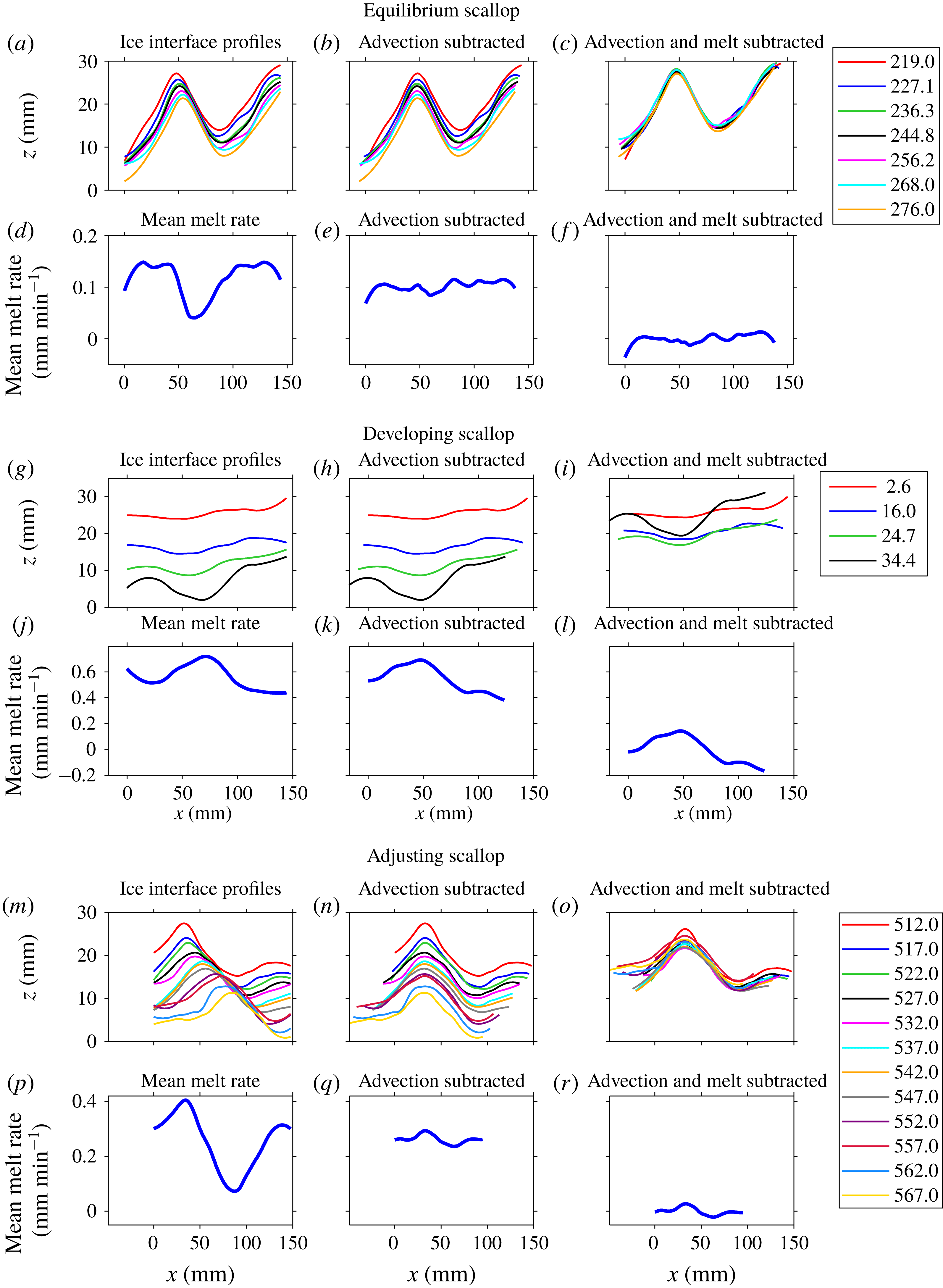
Figure 3(a) shows ice-interface profiles from experiment 1a, after scallops had developed and equilibrated. With each successive measurement, we observe that the ice interface melts downwards and the scallop crest moves to the right (downstream). We also note that the scallops have a geometric asymmetry, with steeper slopes on their leeward side and a shallower slope on their streamward side. In figure 3(d), we plot the time-mean melt rate as a function of
 $x$
(the along-flow direction). We observe significant spatial variation in the melt rate, with a minimum occurring roughly one-quarter wavelength downstream of the crest and a maximum occurring roughly three-quarters of a wavelength downstream. This spatially varying melt rate is the reason for the observed downstream migration of the equilibrium scallop geometry: the ice just downstream of the crest is destined to become a future crest, and the ice just downstream of the trough is destined to become a future trough.
While the scallop position is clearly non-stationary, its geometry is relatively fixed. To examine this more closely, we remove the advective component from the ice profiles. Specifically, we locate the crest positions and compute the mean horizontal crest advection speed
 $c$
. Next, for each time
 $t$
, we let
 $h(x,t)=H(x)$
, and subtract advection by performing the transformation
 $h(x,t)\mapsto H(x-ct)$
. The resulting ice-interface profiles are plotted in figure 3(b), and the corresponding time-mean melt rate is shown in figure 3(e). We observe that, after advection is subtracted, the melt rate is nearly constant along the interface. This indicates that, in this advective frame of reference, the scallop evolves with a roughly constant geometry.
Next, we additionally subtract the effect of the spatial and temporal mean melt rate,
 $-\bar{{\dot{h}}}$
, defined as
 $$\begin{eqnarray}\displaystyle -\bar{{\dot{h}}}=-{\displaystyle \frac{1}{T}}{\displaystyle \frac{1}{{\mathcal{L}}}}\int _{0}^{{\mathcal{L}}}\!\int _{0}^{T}{\dot{h}}(x^{\prime },t^{\prime })\,\text{d}t^{\prime }\,\text{d}x^{\prime }, & & \displaystyle\end{eqnarray}$$
where
 ${\mathcal{L}}$
is the length of the domain and
 $T$
is the time span over which data were collected. To additionally subtract the effect of the mean melt rate, we perform the transformation
 $h(x,t)\mapsto H(x-ct)-\bar{{\dot{h}}}t$
. The resulting ice-interface profiles, with advection and mean melt subtracted, are plotted in figure 3(c). The corresponding time-mean melt rate for these profiles is shown in figure 3(f). We observe that, with the subtraction of interface advection and mean melt, the scallop geometry assumes a roughly universal shape, with the profiles collapsing onto one another. This also implies that any cross-stream evolution of the 3-D scallop features is slow compared with their migration in the downstream direction.
3.2.2 Scallop development
Before reaching its equilibrium scallop geometry, the ice interface undergoes an unstable transition from a flat to a scalloped surface. Depending on the flow speed, this transition takes between 30 and 300 min of experiment time. In figure 3(g–l), we plot analogous quantities to figure 3(a–f), but for a regime of scallop development (data from experiment 2). Figure 3(g) shows interface profiles as the ice evolves from a flat to a scalloped geometry. We observe that the mean melt rate, shown in figure 3(j), has a maximum in the developing scallop trough. Moreover, unlike the equilibrium scallop case, when advection is subtracted (figure 3 h) the melt rates (figure 3 k) remain variable along the interface. Note that, in this experiment, advection was subtracted by finding the position of the scallop troughs, as these were more clearly identifiable than the crests. The spatially variable melt rate in figure 3(k) indicates that this scallop development regime does not have an advective reference frame in which the ice interface maintains its geometry. In other words, after flow is imposed, the ice undergoes an adjustment to a new stable geometry. Similarly, after the subtraction of advection and mean melt (figure 3 l), we do not observe the collapse of the interface profiles to a single shape, as in the equilibrium scallop case, indicating that the ice geometry is in a non-equilibrium state of development.
Ice-interface profiles (upper rows) and melt rates (lower rows) for an equilibrium scallop regime (a–f; experiment 1a), a developing scallop regime (g–l; experiment 2), and a scallop adjustment regime (m–r; experiment 1b). The flow direction is from left to right. The
 $x=0$
location is an arbitrary origin corresponding to the left edge of the field of view in the first dataset collected. The first column shows the raw data, the second column considers profiles where the effect of crest advection has been subtracted, and in the third column crest advection and mean melt rates have been subtracted. Colours indicate different times (measured in minutes) within the experiment. Note that the aspect ratio has been increased to emphasize the scallop geometry.

3.2.3 Scallop adjustment
A third regime of ice melt identified in our experiments is the adjustment of a pre-existing scalloped geometry. This scallop adjustment occurs when the flow conditions that were used to produce a scallop are modified. For example, in experiment 1a, scallops were produced using flow speeds of 1.00 m s
 $^{-1}$
. At the end of the experiment (experiment time of 495.0 min), the flow speed was reduced to 0.16 m s
 $^{-1}$
(experiment 1b), and the subsequent ice interface adjustment is reported here (figure 3
m–r).
We observe a clear downstream migration of the scallop interface (figure 3
m) and highly variable melt rates along this interface (figure 3
p). After subtraction of advection, we observe that melt rates are more uniform (figure 3
q), exhibiting a modest spatial variation, with a local maximum over the crest and a local minimum roughly one-quarter wavelength downstream of the crest. This melt-rate profile acts to preferentially melt the scallop crests, thereby dampening the existing scallop geometry. The adjustment process is illustrated in figure 3(o), which shows interface profiles after advection and mean melt have been subtracted. Unlike the equilibrium scallops of figure 3(c), these profiles do not collapse onto one another, indicating that the interface is undergoing modifications to its geometry and changes to its spatial-mean melt rate
 $\bar{{\dot{h}}}$
.
The adjustment process can also be captured by tracking the path that the scallop crest traverses through
 $x{-}z$
space. Following Blumberg & Curl (Reference Blumberg and Curl1974), we compute a crest evolution angle
 $\unicode[STIX]{x1D719}=\text{arctan}({\dot{h}}/c)$
, defined as the angle between the horizontal and the line connecting successive scallop crests. In the cases of equilibrium and developing scallops shown in figure 3, the values of
 $\unicode[STIX]{x1D719}$
are 40
 $^{\circ }$
and 41
 $^{\circ }$
, respectively, whereas in the adjustment case
 $\unicode[STIX]{x1D719}=15^{\circ }$
. This indicates that scallops adjusting to a slower flow speed have more horizontal advection, relative to their vertical melt rates, than their equilibrium counterparts, possibly due to the adjustment of the interface towards a new equilibrium wavelength. It is possible that
 $\unicode[STIX]{x1D719}$
would increase again once a new equilibrium is established, but our experiments did not run sufficiently long to explore this hypothesis.
3.3 Conditions for scallop equilibrium
Next, we investigate the interaction between ice geometry and melt rates, with the objective of developing understanding of the melt regimes identified above. This analysis does not address fluid dynamical features of the ice–water interaction, which we consider explicitly in the following section. Rather, we utilize given melt-rate profiles taken from the experiments, which can be thought of as the net outcome of fluid dynamical processes on the ice. Here we seek to identify the conditions under which a given ice geometry will propagate stably when subjected to a specified melt-rate profile.
Suppose that we have an initial ice geometry
 $h(x,t=0)=G(x)$
and are given a fixed melt-rate profile
 $F(x)$
. First, we know that if the melt-rate profile is non-constant and fixed in space, then the ice will melt unstably, with the deepest points growing continually deeper. Therefore, the maintenance of a fixed scallop geometry requires the movement of this melt-rate profile relative to the ice interface. We let
 $c$
be the horizontal advection speed of the melt-rate profile, and assume that
 $c$
has a constant value. Therefore, the time-evolving melt rate in this model is given by
 $-{\dot{h}}(x,t)=F(x-ct)$
. Now, we ask: Given this advecting melt-rate profile, what initial ice geometries
 $G(x)$
will evolve in equilibrium as
 $h(x,t)=G(x-ct)$
? We choose the same
 $c$
because we expect that ice geometry sets the properties of ice–water boundary-layer turbulence and the corresponding melt rates, and therefore the ice geometry and melt rates should advect at the same rate. For these conditions to be simultaneously satisfied, we must have that
 $-{\dot{h}}(x,t)=cG^{\prime }(x-ct)=F(x-ct)$
. At
 $t=0$
, we have
 $cG^{\prime }(x)=F(x)$
. Integrating in
 $x$
, we find that
 $$\begin{eqnarray}\displaystyle G(x)={\displaystyle \frac{1}{c}}\int _{0}^{x}F(x^{\prime })\,\text{d}x^{\prime }+C. & & \displaystyle\end{eqnarray}$$
Therefore, given a melt-rate profile and an advection speed
 $c$
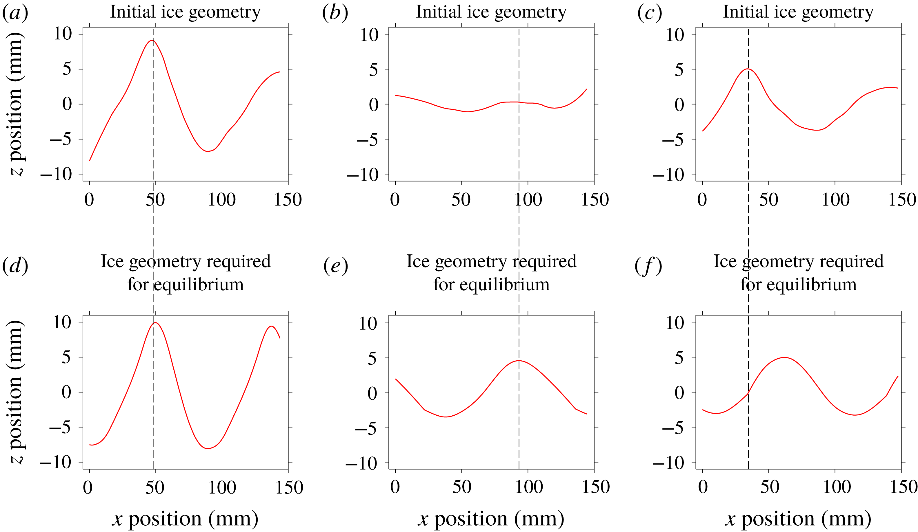
, this condition provides the initial ice geometry that will evolve in equilibrium. This can be applied directly to the observed melt rates and advection speeds from § 3.2 to compute the initial ice-interface geometries that would be required for equilibrium evolution. Comparing these hypothetical ice geometries to the actual initial ice geometries (see figure 4) provides information on the degree to which a given experiment has evolved to equilibrium. In particular, we find that, in the case of scallop development and adjustment (figures 4
b,e and 4
c,f, respectively), the initial profiles have a significant mismatch with the equilibrium profiles computed using (3.7), in terms of their amplitude and crest position, respectively. On the other hand, the equilibrium scallop case shows a good match between the two, indicating that it is indeed evolving in an equilibrium state.
Initial ice geometry required for equilibrium scallops (d–f; computed using condition (3.7)), and the actual initial ice geometry from the experiment (a–c). Shown are three cases: scallop equilibrium (a,d; experiment 1a), development (b,e; experiment 2), and adjustment (c,f; experiment 1b). The dashed vertical lines indicate the crest position of the initial geometry in the experiments (a–c), which can be compared to the crest position required for equilibrium scallops (d–f).

4 Flow measurements in an evolving ice–ocean boundary layer
4.1 Velocity field characteristics
In this section, we use laboratory PIV data to study the characteristics of the 2-D flow field,
 $\boldsymbol{u}=(u,w)$
, over a time-evolving ice–water interface. We begin by analysing time-mean velocity fields from experiment 3 in two contrasting ice geometries: (1) flat ice; and (2) a fully developed scallop.
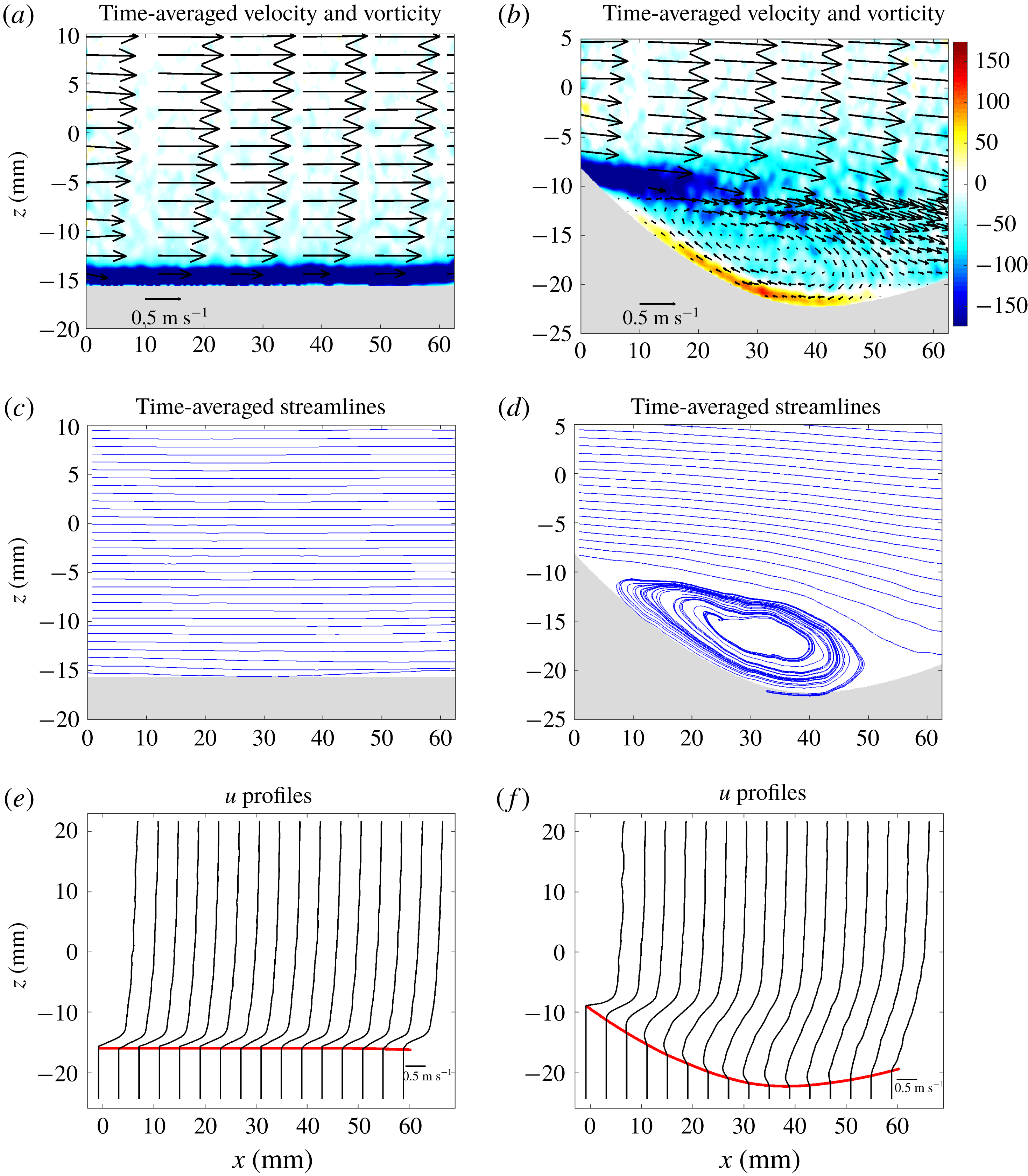
In figure 5, we plot the time-averaged velocity,
 $(\bar{u},\bar{w})$
, vorticity,
 $\bar{\unicode[STIX]{x1D701}}=\unicode[STIX]{x2202}\bar{w}/\unicode[STIX]{x2202}x-\unicode[STIX]{x2202}\bar{u}/\unicode[STIX]{x2202}z$
, and streamfunction,
 $\bar{\unicode[STIX]{x1D713}}$
, over flat and scalloped ice. The flat-ice velocity field is nearly uniform in
 $x$
, has little vertical velocity, and has a thin (2 mm) strip of negative vorticity which arises from the no-slip boundary condition at the ice–water interface. The velocity field displays a boundary-layer structure, which we investigate in detail below. The scalloped-ice geometry creates a clear modification to the flow field, dominated by a recirculating eddy that encompasses most of the scallop trough. This clockwise-rotating eddy has a length : height aspect ratio of roughly 5 : 1 and produces a negative vorticity field throughout most of the scallop trough. The no-slip boundary condition at the scallop crest acts as a source of negative vorticity, from which clockwise-rotating eddies are shed. There is also a thin strip of positive vorticity at the ice–water interface in the scallop trough, which arises due to the reverse flow of the recirculating eddy. In the time mean, the scallop trough is relatively quiescent compared to the free-stream flow: a typical velocity in the trough is 0.20 m s
 $^{-1}$
and the free-stream velocity is roughly 0.90 m s
 $^{-1}$
. This time-mean flow suggests a flow-driven mechanism for scallop creation, in which eddies act to preferentially transport heat into the scallop trough relative to the crests. Depending on the ice geometry, this flow field and corresponding heat transfer can either act to self-reinforce and grow an ice roughness element, or maintain an existing scallop. Our quantitative time-mean laboratory data closely resemble the sketch for a scallop flow-driven mechanism presented in Blumberg & Curl (Reference Blumberg and Curl1974).
Time-averaged velocity (vectors), vorticity (colour), streamlines and
 $u$
-velocity profiles over flat (a,c,e) and scalloped (b,d,f) ice from experiment 3. The ice–water interface in (e) and (f) is indicated in red and the vertical lines below the interface indicate
 $u=0$
values.

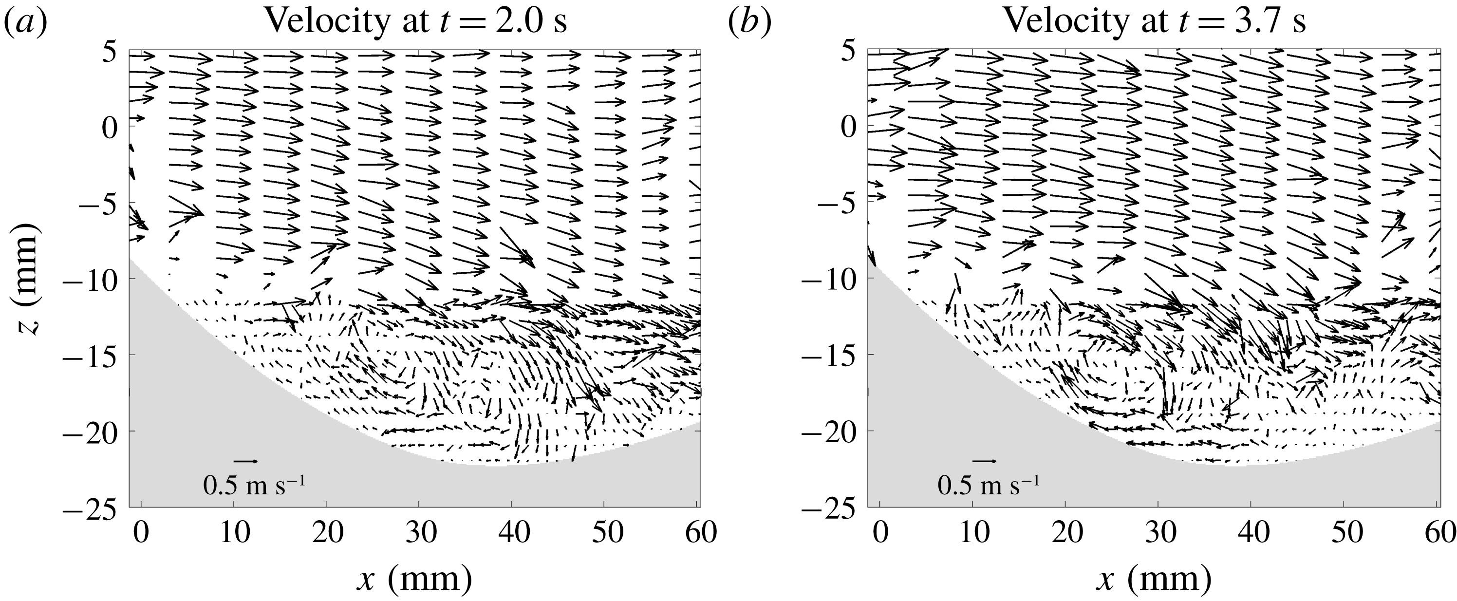
Snapshots of the instantaneous flow field over a scallop at different times from experiment 3.

It is important to note that, while the time-mean velocity field shows a clear recirculating flow pattern, any given snapshot of the field deviates from this substantially. To demonstrate this temporal variability, in figure 6 we show instantaneous snapshots of the velocity field over a scalloped geometry. Each of these snapshots is distinct, particularly in the scallop trough region, indicating that the scallop flow is highly transient near the ice–water interface. The snapshots are noisier, display more fine-scale structure and have larger trough velocities than their time-mean counterpart. Despite the differences between snapshots, each field displays a key common feature: a flow reversal that occurs within the scallop trough, which drives a reverse flow up the leeward side of the scallop. The recirculating eddies in these snapshots have varying spatial positions and tend to be more circular than the recirculating eddy in the time-mean flow. This highlights the important point that the time-mean velocity field is the result of averaging over a multitude of individual eddy and flow reversal events. These snapshots also provide an indication of the PIV data quality. Each snapshot field has some spurious vectors, but these errors tend to cancel out under time averaging. We return to the key role of transient flow features in scallop formation in § 4.3 below.
To further investigate the influence of a scalloped-ice geometry on the time-mean flow, we perform a decomposition
 $$\begin{eqnarray}\displaystyle \bar{\boldsymbol{u}}=[\bar{\boldsymbol{u}}]+\bar{\boldsymbol{u}}^{S}, & & \displaystyle\end{eqnarray}$$
where
 $[\cdot ]$
is an average along the
 $x$
-dimension, and
 $^{S}$
represents the deviation from this mean, often called the stationary eddy component. To perform this decomposition, we first change variables to a terrain-following vertical coordinate,
 $\unicode[STIX]{x1D70E}\in [0,1]$
. The transformation
 $(x,z)\mapsto (x,\unicode[STIX]{x1D70E})$
is given by
 $$\begin{eqnarray}\displaystyle \unicode[STIX]{x1D70E}={\displaystyle \frac{z-h(x)}{z_{top}-h(x)}}, & & \displaystyle\end{eqnarray}$$
where
 $z_{top}$
is the height of the optical coupler (with typical value of roughly 300 mm) and
 $h(x)$
is the ice–water interface. The value
 $\unicode[STIX]{x1D70E}=0$
corresponds to the ice–water interface, and
 $\unicode[STIX]{x1D70E}=1$
corresponds to the top of the field of view. The
 $x$
-average,
 $[\cdot ]$
, is computed along constant-
 $\unicode[STIX]{x1D70E}$
surfaces. This averaging technique is more robust to noise than using constant-
 $z$
surfaces, and has the advantage of associating points based on a physically relevant quantity: their distance from the ice–water interface.
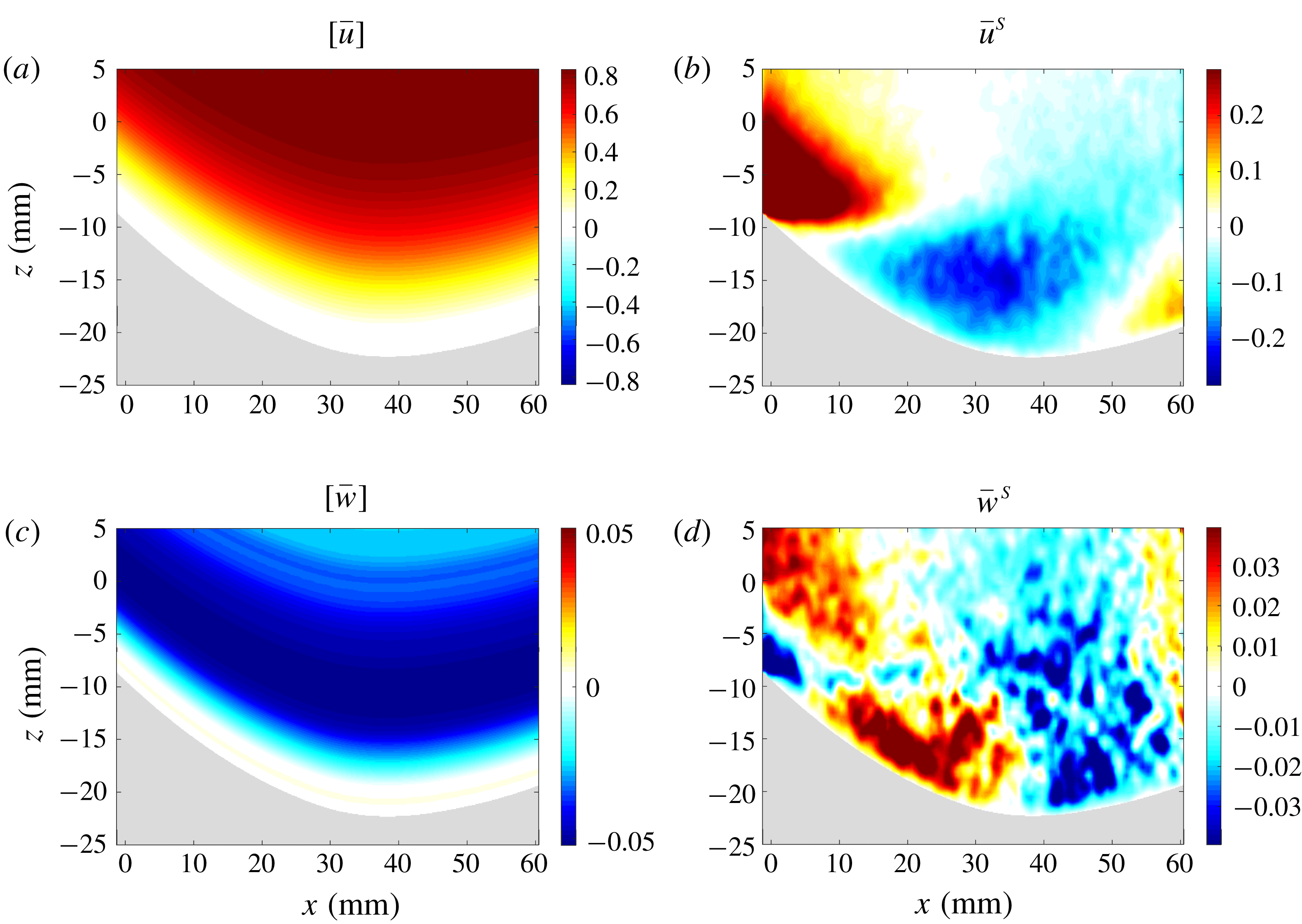
Decomposition of the time-mean scallop flow into an along-flow mean, (
 $[\bar{u}]$
,
 $[\bar{w}]$
), and a standing eddy component, (
 $\bar{u}^{S}$
,
 $\bar{w}^{S}$
). These data are from experiment 3.

We plot the decomposed time-mean velocity fields for a scalloped-ice geometry in figure 7. The
 $[u]$
values increase monotonically away from the interface, whereas the
 $[w]$
values are negative and strongest roughly 10 mm above the interface, indicating general downwelling near the scallop depression. The standing eddy component, (
 $\bar{u}^{S}$
,
 $\bar{w}^{S}$
), reflects deviations from this along-flow mean. Consistent with the flow reversal in figure 5, the
 $\bar{u}^{S}$
velocities are negative in the scallop trough, whereas the
 $\bar{w}^{S}$
velocities indicate upwelling upstream of the trough minimum and downwelling downstream of this minimum. The regions of anomalous downwelling and upwelling correspond to the regions of maximum and minimum melt, respectively, within a scallop trough (see figure 3). This suggests that this standing eddy pattern contributes to the differential melt rates along the ice–water interface and the downstream advection of the scalloped geometry.
4.2 Boundary-layer structure
We next consider the effect of ice geometry on the structure of the ice–water boundary layer. In figure 5(e,f), we plot time-mean profiles of the
 $u$
-velocity component over flat and scalloped ice. The flat-ice profiles display high levels of vertical shear immediately adjacent the ice–water boundary. Above this high-shear zone, the velocities increase much more slowly with height, obeying a logarithmic velocity profile, which we explore below. The scalloped-ice geometry has a clear influence on the ice–water boundary layer. Unlike the flat-ice case, the scallop boundary-layer profiles vary strongly according to their position within the scallop. At the scallop crest, there is a high level of vertical shear near the ice interface. At this location, the boundary-layer profiles resemble the flat-ice case, but have stronger vertical shear. Moving into the scallop interior, the vertical shear weakens substantially, indicating smaller velocities in the scallop trough region. Additionally, the boundary-layer profiles assume negative values near the ice interface in the scallop trough, indicating the flow reversal that occurs within the scallop. The loss of vertical shear within a scallop trough is a crucial element of scallop formation, which we explore in § 4.3 below.
Turbulent boundary layers near a wall display a well-known logarithmic velocity profile known as the ‘law of the wall’. The law of the wall for a velocity profile
 $u(z)$
adjacent to a flat, hydraulically smooth wall is given by
 $$\begin{eqnarray}\displaystyle u(z)={\displaystyle \frac{u_{\ast }}{\unicode[STIX]{x1D705}}}\,\text{ln}(z)+B, & & \displaystyle\end{eqnarray}$$
where
 $\unicode[STIX]{x1D705}$
is the von Kármán constant,
 $u_{\ast }=\sqrt{\,\overline{u^{\prime }w^{\prime }}\,}$
is the friction velocity and
 $B$
is a constant. Defining non-dimensional velocity and height variables given by
 $u^{+}=u/u_{\ast }$
and
 $z^{+}=z/\unicode[STIX]{x1D708}/u_{\ast }$
, this equation becomes
 $$\begin{eqnarray}\displaystyle u^{+}={\displaystyle \frac{1}{\unicode[STIX]{x1D705}}}\,\text{ln}(z^{+})+C, & & \displaystyle\end{eqnarray}$$
where
 $C$
is a constant (Schlichting et al.
Reference Schlichting, Gersten, Krause, Oertel and Mayes1960). Very close to the wall, viscous effects dominate and the velocities follow a linear profile given by
 $$\begin{eqnarray}\displaystyle u^{+}=z^{+}. & & \displaystyle\end{eqnarray}$$
This ‘viscous sublayer’ region applies for
 $0<z^{+}<5$
, whereas the logarithmic layer applies for
 $z^{+}>30$
. The region defined by
 $5<z^{+}<30$
is referred to as the ‘buffer layer’, which provides a smooth transition between the linear and logarithmic velocity regimes (Schlichting et al.
Reference Schlichting, Gersten, Krause, Oertel and Mayes1960).
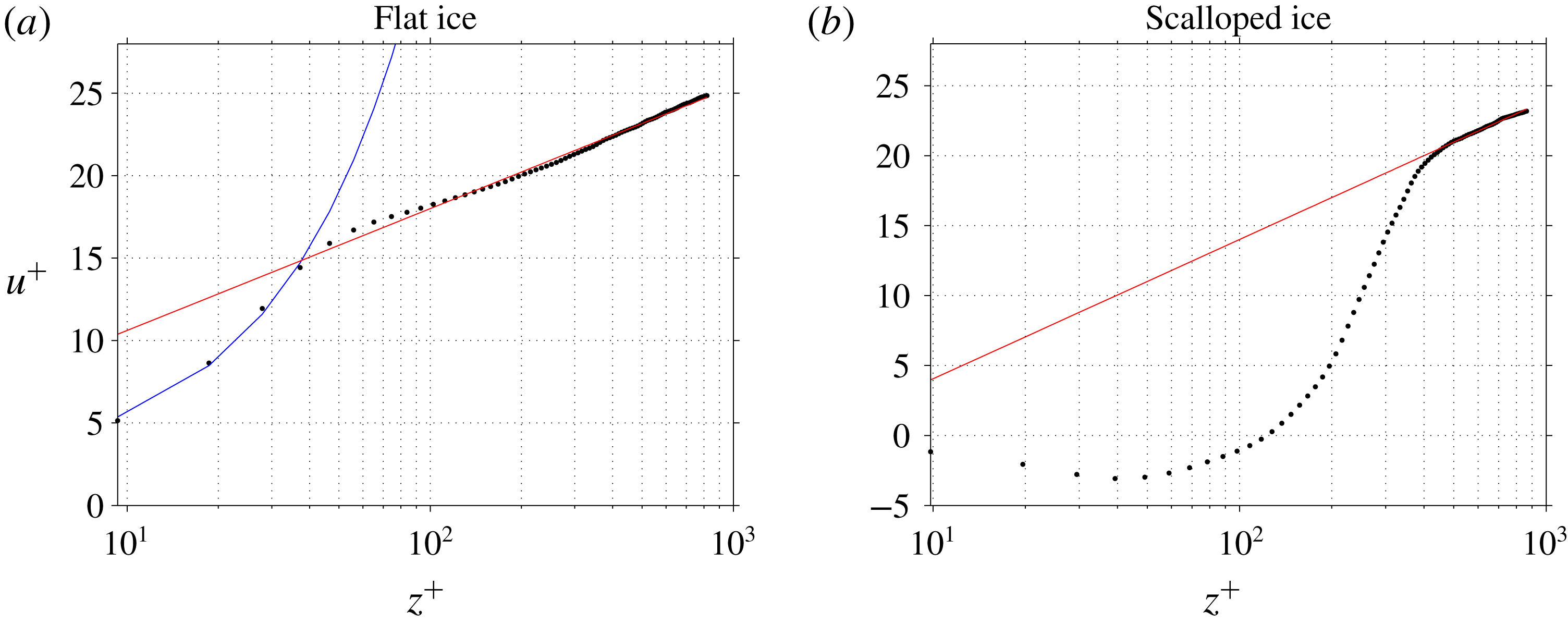
Law-of-the-wall relationship over flat ice and scalloped ice from experiment 3. The non-dimensional velocity
 $u^{+}$
is plotted as a function of the logarithm of the non-dimensional distance
 $z^{+}$
. The blue curve is a linear fit to the near-ice data points, and the red curve is a logarithmic fit to the data points in the ‘log-law’ region. For the flat-ice case, the velocities have been averaged between
 $x=0$
and
 $60$
. The scallop velocities have been averaged between
 $x=20$
and
 $40$
, the primary region of recirculation within the scallop trough. The hydraulic roughnesses are 0.016 mm and 0.16 mm for flat and scalloped ice, respectively.

In figure 8, we examine the agreement of our laboratory PIV data with the law-of-the-wall theory. To do this, we perform a direct computation of
 $u_{\ast }$
by averaging the kinematic shear stress values,
 $\overline{u^{\prime }w^{\prime }}$
, over the near-wall region in which these values are roughly constant. Specifically, we average over the region between
 $z=10$
and
 $z=20$
mm (see figure 5
e,f), which yields values of
 $u_{\ast }=0.04$
m s
 $^{-1}$
for both the flat- and scalloped-ice cases, respectively. The corresponding viscous length scale is given by
 $\unicode[STIX]{x1D708}/u_{\ast }=0.04$
mm, where
 $\unicode[STIX]{x1D708}=1.6\times 10^{-6}$
m
 $^{2}$
s
 $^{-1}$
is the kinematic viscosity of water at 0
 $^{\circ }$
C. Our data, with resolution of 0.4 mm, are unable to resolve the viscous sublayer. A specialized future study with very high vertical resolution would be required to properly probe this layer. We compute a velocity profile
 $u^{+}$
at each
 $x$
-location along the ice–water interface, and then compute the average of these profiles. For the flat-ice case, the
 $u^{+}$
profiles are uniform in
 $x$
, so the averaging is performed over the entire ice–water interface. Conversely, the
 $u^{+}$
profiles over scalloped ice vary strongly in
 $x$
, and therefore are sensitive to the averaging window. The vertical coordinate used for averaging is the (non-dimensional) distance from the ice–water interface (i.e. the averaging is performed over surfaces with constant distance from the ice–water interface).
The PIV data collected over flat ice reveal a clear law-of-the-wall boundary-layer structure, with velocity increasing logarithmically for
 $z^{+}>30$
(see figure 8
a). For values of
 $10<z^{+}<30$
, the velocities increase roughly linearly (which corresponds to an exponential shape in this linear–log plot). This region of roughly linear velocity increase is the buffer layer, which smoothly joins the logarithmic layer with the viscous sublayer. The scalloped-ice case also displays a logarithmic velocity layer, but only in the far field (
 $z^{+}>400$
when the averaging is performed between
 $x=20$
and
 $x=40$
, the primary region of recirculation within the scallop trough; for
 $u^{+}$
profiles at different
 $x$
locations in the scallop trough, see supplementary figure S1). Near the ice–water interface the velocities approach zero from the negative side, joining the reverse flow of the scallop trough to the viscous sublayer. For values of
 $50<z^{+}<300$
, the velocities increase roughly linearly, adjusting to the far-field logarithmic layer. The scalloped-ice geometry produces a clear modification to the boundary-layer flow, which has important implications for differential melt rates along the ice–water interface. We explore this next.
4.3 Turbulent kinetic energy: interaction between shear production and ice geometry
In this subsection, we consider the interaction between ice geometry and turbulent kinetic energy (TKE) in the ice–ocean boundary layer. We examine the role of TKE production via shear in driving the formation and downstream propagation of ice scallops. For the 2-D incompressible flow considered here, the TKE (denoted by
 $e$
) is given by
 $$\begin{eqnarray}\displaystyle e={\textstyle \frac{1}{2}}(u^{\prime }u^{\prime }+w^{\prime }w^{\prime }), & & \displaystyle\end{eqnarray}$$
where
 $\boldsymbol{u}^{\prime }=\boldsymbol{u}-\bar{\boldsymbol{u}}$
. The time-mean velocity
 $\bar{\boldsymbol{u}}$
is computed over the data acquisition period for a given ice geometry (i.e. 6.7 s and 100 velocity samples for these experiments). The evolution of time-mean TKE,
 $\bar{e}$
, is given by
 $$\begin{eqnarray}\displaystyle {\displaystyle \frac{\unicode[STIX]{x2202}\bar{e}}{\unicode[STIX]{x2202}t}}+\bar{\boldsymbol{u}}\boldsymbol{\cdot }\unicode[STIX]{x1D735}\bar{e}=S+T+B+D, & & \displaystyle\end{eqnarray}$$
where
 $S$
,
 $T$
,
 $B$
and
 $D$
are the shear production, transport, buoyancy production and dissipation terms, respectively. These terms are given by
 $$\begin{eqnarray}\displaystyle & \displaystyle S=-\overline{u_{i}^{\prime }u_{j}^{\prime }}\,{\displaystyle \frac{\unicode[STIX]{x2202}\overline{u_{i}}}{\unicode[STIX]{x2202}x_{j}}},\quad T=-{\displaystyle \frac{\unicode[STIX]{x2202}}{\unicode[STIX]{x2202}x_{j}}}\left[\overline{u_{j}^{\prime }e^{\prime }}+{\displaystyle \frac{1}{\unicode[STIX]{x1D70C}}}\overline{u_{j}^{\prime }p^{\prime }}-\unicode[STIX]{x1D708}\overline{u_{i}^{\prime }\left({\displaystyle \frac{\unicode[STIX]{x2202}u_{i}^{\prime }}{\unicode[STIX]{x2202}x_{j}}}+{\displaystyle \frac{\unicode[STIX]{x2202}u_{j}^{\prime }}{\unicode[STIX]{x2202}x_{i}}}\right)}\right], & \displaystyle\end{eqnarray}$$
 $$\begin{eqnarray}\displaystyle & \displaystyle B=\overline{w^{\prime }b^{\prime }},\quad D=-\unicode[STIX]{x1D708}\overline{{\displaystyle \frac{\unicode[STIX]{x2202}u_{i}^{\prime }}{\unicode[STIX]{x2202}x_{j}}}\left({\displaystyle \frac{\unicode[STIX]{x2202}u_{i}^{\prime }}{\unicode[STIX]{x2202}x_{j}}}+{\displaystyle \frac{\unicode[STIX]{x2202}u_{j}^{\prime }}{\unicode[STIX]{x2202}x_{i}}}\right)}, & \displaystyle\end{eqnarray}$$
 $i,j$
indices are used to denote velocity and coordinate components, and repeated indices are summed over.
The buoyancy production term is small for this experiment (typical values of
 ${<}10^{-7}$
, compared to
 $O(1)$
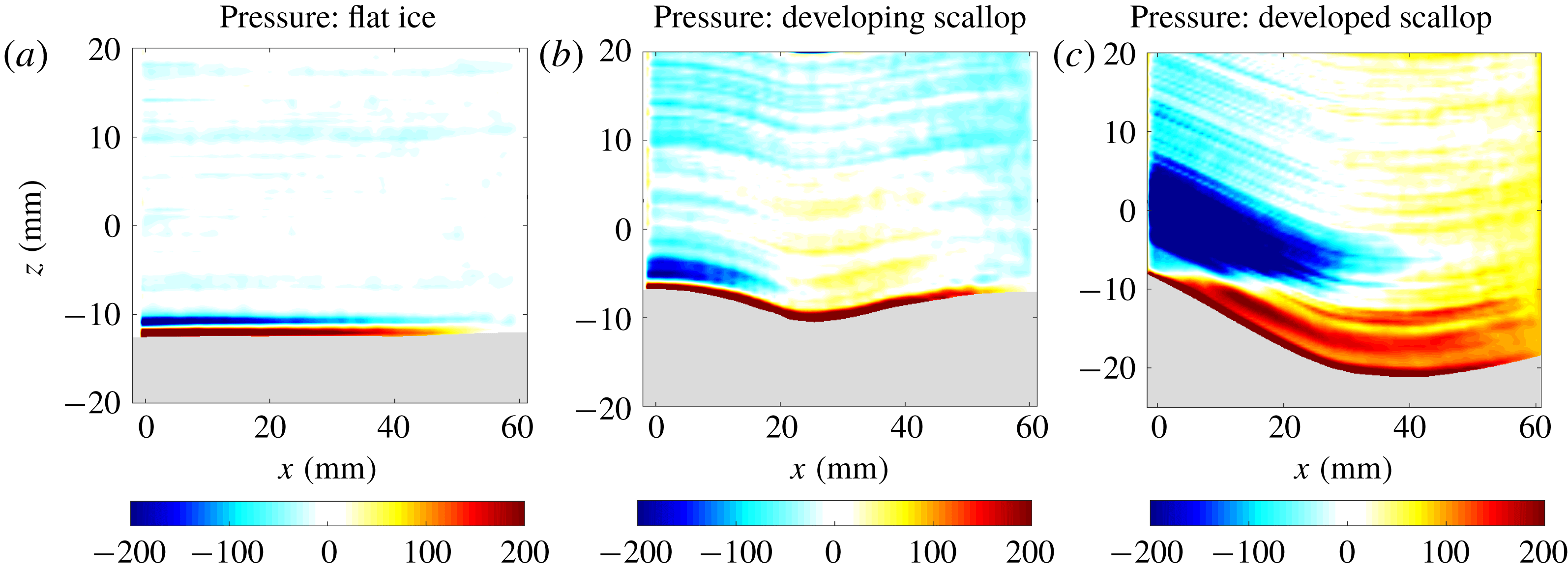
shear production values), and therefore we neglect it in this analysis. The transport term, involving a derivative of the covariance of velocity and TKE fluctuations, velocity and pressure fluctuations, and a viscous transport term, is challenging to measure accurately given the triple correlations and pressure fluctuations that appear in this term. In order to compute the pressure term, we compute all other terms in the momentum equation (3.1) using the measured velocities. This yields a pressure gradient field, which can be spatially integrated to obtain the time-varying pressure field. Using this method, we directly computed the transport term, but found that it was too noisy to interpret reliably (see figure S2). This noise is likely a combination of experimental noise (i.e. errors in our PIV-derived velocity vectors) and sampling error (i.e. not having enough velocity samples to reliably compute triple temporal covariances). Similarly, our data do not have sufficient spatial resolution to reliably estimate the dissipation term
 $D$
, as the dissipation length scale corresponding to typical velocity fluctuations,
 $\unicode[STIX]{x1D708}/u^{\prime }$
, is smaller than the resolution of our data. We find that the computed dissipation term closely resembles the spatial structure of the TKE field, but this may have errors associated with resolution (see figure S2). Future work, focused on accurately measuring and computing the transport and dissipation terms, is required. The shear production term comprises four distinct terms, with the dominant contribution coming from the
 $S_{xz}=-\overline{u^{\prime }w^{\prime }}(\unicode[STIX]{x2202}\overline{u}/\unicode[STIX]{x2202}z)$
term, which is the TKE production resulting from vertical shear of the horizontal mean flow. Computing this term is more robust than the transport and dissipation terms, since the mean flow varies over larger spatial scales. The other shear production terms are generally smaller in magnitude, less spatially coherent, and have higher levels of numerical noise (see figure S2). We also note that these 2-D velocity measurements are unable to assess TKE contributions associated with out-of-plane velocity fluctuations, which are likely an important aspect of 3-D scallop formation. For the present analysis, we focus on the TKE and the
 $S_{xz}$
shear production term.
TKE (m
 $^{2}$
s
 $^{-2}$
) and shear production (m
 $^{2}$
s
 $^{-3}$
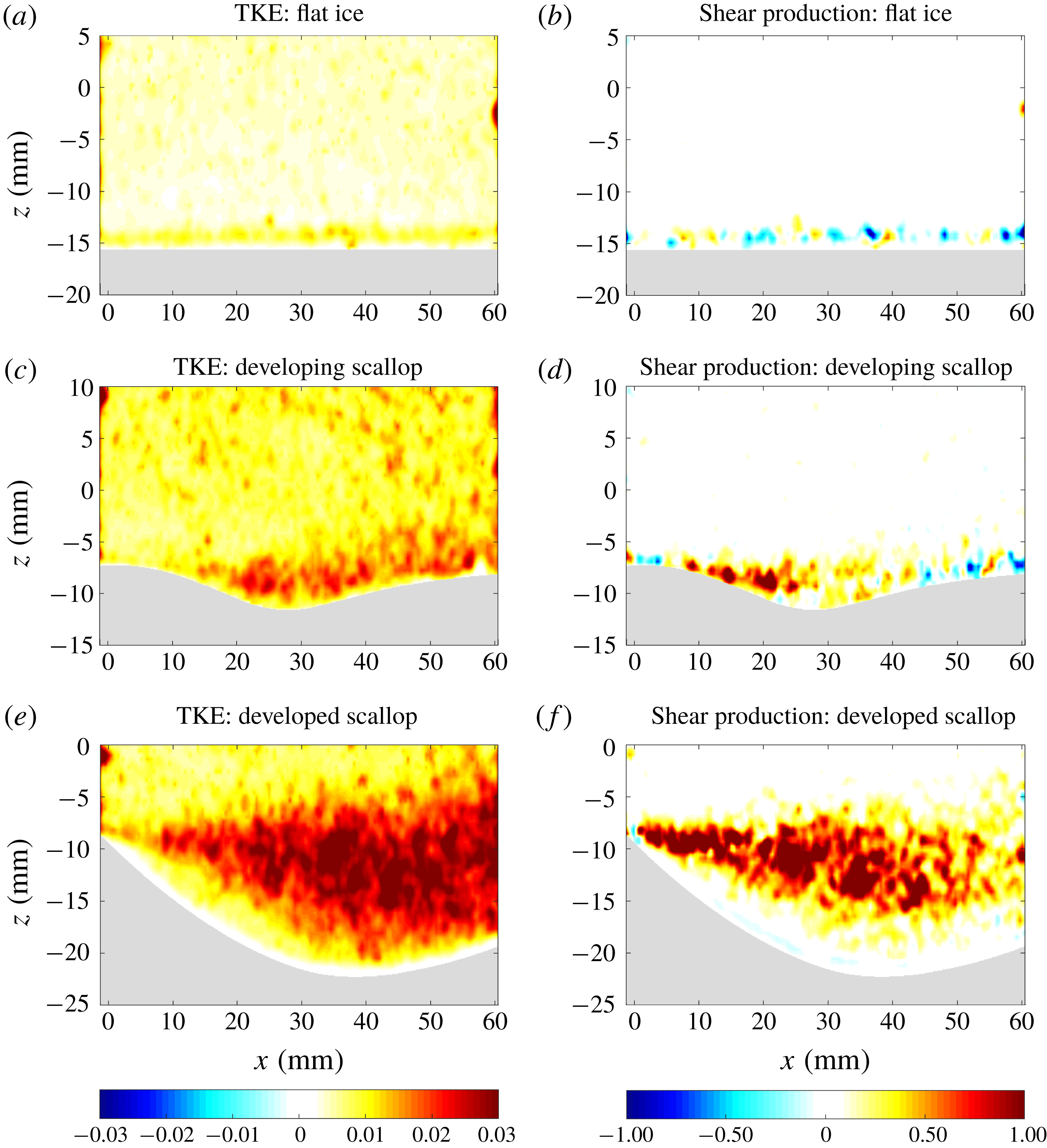
) measurements over flat ice (a,b), a developing scallop (c,d) and a fully developed scallop (e,f) from experiment 3.

In figure 9, we consider the evolution of TKE and
 $S_{xz}$
from experiment 3, as an initially flat ice–water interface develops into a scalloped geometry. The initially flat ice (figure 9
a,b) has a relatively uniform TKE distribution, aside from a small 2 mm strip of higher TKE at the ice–water interface. The shear production term over this flat interface is small, and does not display a coherent spatial structure. As the ice–water interface begins to develop a scalloped geometry (figure 9
c,d), there are notable changes to each of these fields. In particular, the TKE field develops high values in the scallop trough and along its streamward slope, with relatively lower values above and just downstream of the scallop crest. In contrast, the region of high shear production is spatially distinct, with high shear production values originating from the scallop crest and extending roughly to the middle of the scallop trough, beyond which the values are reduced.
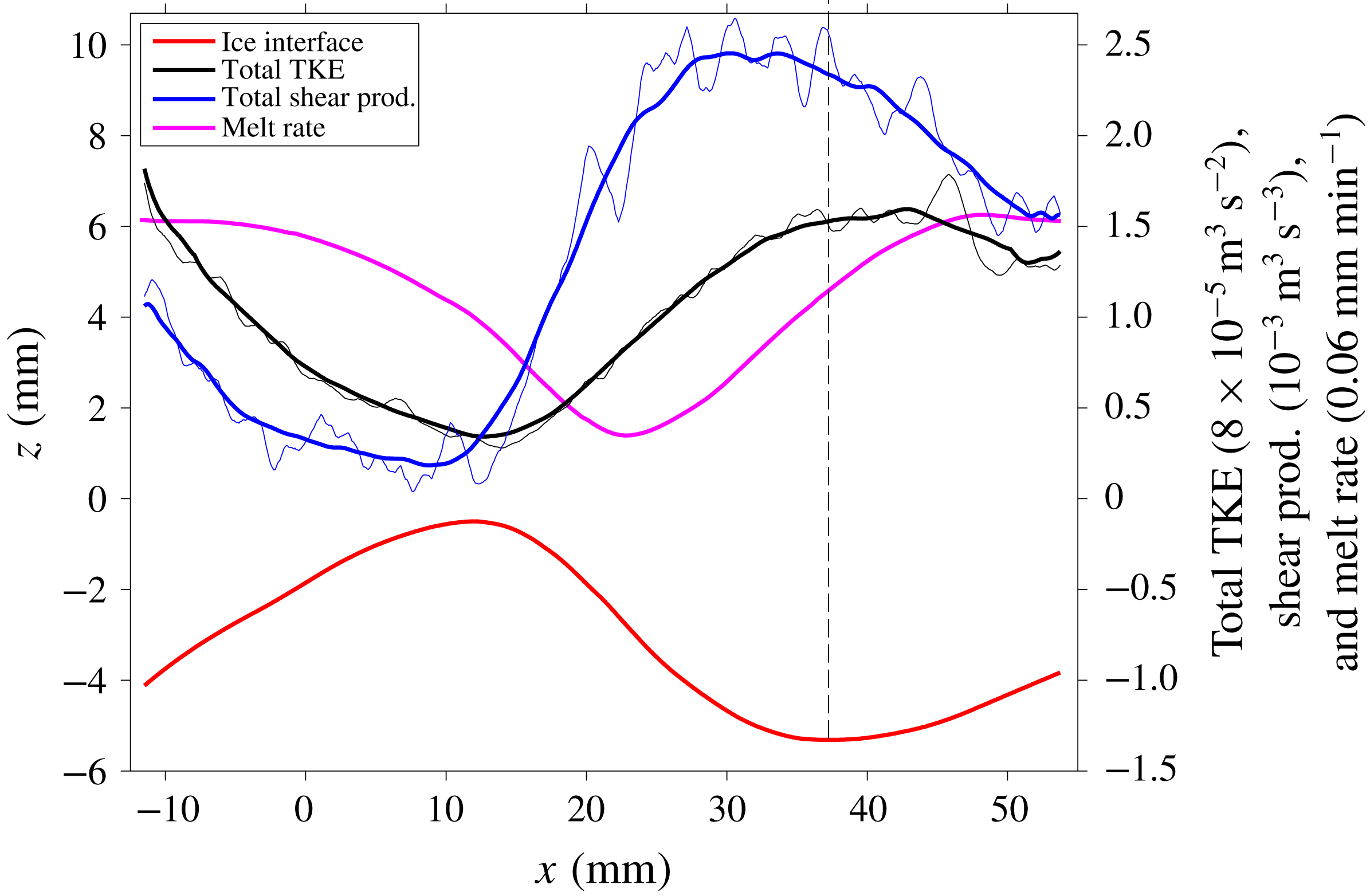
Analogous features can be seen more strikingly in the fully developed scallop in figure 9(e,f). The TKE field displays a flow separation occurring at the scallop crest, with a transition to turbulence occurring roughly 10 mm downstream of this separation point. The region of high TKE spreads out within the scallop trough, reaching its maximum values just downstream of the trough minimum. This TKE field acts to mix water temperatures down their mean gradient, tending to mix relatively warm water downwards towards the ice–water interface. Thus, the location of maximum TKE should correspond roughly to the location of maximum turbulent heat transfer, which is consistent with the observed maximum melt rates occurring just downstream of the scallop trough minimum. Additionally, the TKE values are lowest along the leeward slope of the scallop, consistent with the observed minimum melt rates at this location. We also note that the maximum melt rates coincide with the location of maximum downward advection by the time-mean recirculating flow (see figures 5 and 7), suggesting that there are likely melt-rate contributions from both the time-mean and the transient flow. The dominant source of scallop TKE is the production of TKE via vertical shear of the horizontal flow in the flow interior. The shear production is particularly high near the separation point at the scallop crest, and has high values extending to roughly the scallop trough minimum position, notably upstream of the maximum TKE location. The relative spatial distributions of the TKE and shear production terms are considered quantitatively in figure 11 below. We also note that experimental measurements of TKE and shear production over subaqueous sediment ripples similarly show maxima in these fields near the trough minimum position (Nelson et al. Reference Nelson, McLean and Wolfe1993); however, the interface geometry of these ripples is notably distinct from ice scallops, with steeper leeward slopes and shallower streamward slopes.
TKE (m
 $^{2}$
s
 $^{-2}$
) and shear production (m
 $^{2}$
s
 $^{-3}$
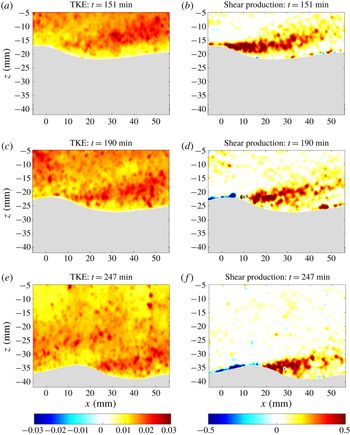
) measurements over an equilibrium scallop from experiment 4 at different experiment times: 151 min (a,b), 190 min (c,d), and 247 min (e,f).

We next consider the evolving TKE distribution of an equilibrium scallop geometry from experiment 4 (figure 10). As the ice interface melts downwards and the scallop crest migrates downstream, we observe a clear migration of the region of high shear production, illustrating the crucial importance of the scallop crest position in setting the region of high TKE. Again, we find relatively low TKE values at and immediately downstream of the scallop crest, and higher values downstream of the trough minimum location. We find negative shear production values along the streamward slope of the scallop and high positive values extending from the scallop crest to roughly the trough minimum. This relationship between ice geometry and TKE production via vertical shear in the flow interior suggests a self-reinforcing mechanism for scallop formation, which we discuss next.
4.4 A mechanism for scallop formation
Vertically integrated TKE (black) and shear production (blue) averaged over seven datasets collected near an equilibrium scallop geometry (red). The thick black and blue lines are running horizontal means computed over 8 mm bins. The melt rate is shown in magenta. The TKE and melt-rate curves have been shifted down for visual clarity (by 0.19 mm min
 $^{-1}$
and
 $1.2\times 10^{-4}~\text{m}^{3}~\text{s}^{-2}$
, respectively). The vertical dashed line is a reference to the scallop trough minimum position. These data are from experiment 4.

We quantify the net effect of TKE and shear production in the ice–water boundary layer by considering vertical integrals of these fields. The vertical integrals are computed from the ice interface to a height 10 mm above the scallop crest for seven datasets collected over an equilibrium scallop geometry from experiment 4. We reference the integrated TKE and shear production to a common Lagrangian point on the ice interface (the scallop crest) and average across the seven datasets in figure 11. These data cover nearly a full scallop wavelength and reveal the periodic turbulent flow features that occur near a scalloped surface. We find that the shear production term increases rapidly beginning at the scallop crest, reaching its maximum value prior to the trough minimum position. Beyond the trough minimum, the shear production values decrease monotonically along the streamward slope of the scallop and reach their minimum value at the scallop crest, at which point the flow pattern repeats itself. The integrated TKE is also periodic, but reaches its maximum value slightly downstream of the trough minimum, suggesting that the TKE produced via shear is advected downstream by the mean flow. Interestingly, the location of maximum TKE does not correspond directly to the location of maximum melt rates, which occurs slightly downstream of the TKE maximum. The melt-rate curve closely resembles a phase-shifted version of the TKE curve, indicating that the heat mixed downwards by turbulent eddies experiences some downstream transport before ultimately being transferred to the ice interface. The TKE maximum also coincides with the location of time-mean downward advection, which likely also contributes to the melt rates. These results have some minor sensitivity to the choice of vertical integration domain, but the identified phase relationships between shear production, TKE and melt rates are robust with respect to this choice.
Figure 11 suggests that scallops form and persist due to a periodic self-reinforcing feedback between ice geometry and the turbulent flow field. In this mechanism, the scallop crest is crucially important, acting as a source of TKE via the high vertical shear at this location. The turbulent eddies produced from this TKE source serve two critical functions in forming a scalloped geometry. Firstly, these eddies increase the vertical mixing of heat towards the ice–water interface, thereby driving increased melt rates downstream of the crest. Secondly, these eddies act to erode the vertical shear of the mean horizontal flow (see figure 5 f). This reduction in vertical shear removes the source of TKE, ultimately resulting in a reduction of heat transfer downstream of the melt-rate maximum. The location at which the shear production term begins to weaken corresponds roughly to the scallop trough minimum position. There is a clear phase relationship between the shear production, TKE and melt rate, with the shear production peaking first, followed by the TKE, followed by the melt rate. Downstream of the melt-rate maximum, as the ice geometry rises up to the next crest, a zone of high vertical shear of the horizontal flow is re-established, creating a new source of TKE to drive melting in the subsequent scallop. This periodic relationship between ice geometry, TKE production via vertical shear and melt rates describes a self-reinforcing mechanism for scallop formation and evolution. This analysis suggests that the length of the high shear production region is the critical factor in determining the wavelength of a scallop. Future work is required to examine the controls on the length of this shear production region and its dependence on Reynolds number.
Earlier work by Thorsness & Hanratty (Reference Thorsness and Hanratty1979a
,Reference Thorsness and Hanratty
b
) and Hanratty (Reference Hanratty1981) puts forth an alternative hypothesis that the final scallop wavelength is determined by linear instability properties of the initially flat interface rather than by characteristics of the separated turbulent flow. In particular, their 2-D linear stability analysis provides a prediction for the range of most unstable wavelengths and the corresponding phase angles between the melt-rate profile and the ice-interface geometry. We note that our measured scallop Reynolds number from experiment 4 of
 $\unicode[STIX]{x1D706}u_{\ast }/\unicode[STIX]{x1D708}=2800$
is broadly consistent with the predicted range of most unstable scallop Reynolds numbers of
 $3100<\unicode[STIX]{x1D706}u_{\ast }/\unicode[STIX]{x1D708}<6300$
from Thorsness & Hanratty (Reference Thorsness and Hanratty1979a
). Also, this Reynolds number of 2800 corresponds to a predicted phase angle of approximately 120
 $^{\circ }$
(see figure 9 of Thorsness & Hanratty (Reference Thorsness and Hanratty1979a
)), which is also broadly consistent with the observed phase angle of 140
 $^{\circ }$
(see figure 11). Recent work by Claudin et al. (Reference Claudin, Durán and Andreotti2017) provides predictions for both the wavelength and amplitude of 2-D ripple patterns, predicting an aspect ratio of roughly 2 % for a Reynolds number of 2800. This aspect ratio is considerably smaller than the observed 8 % aspect ratio, suggesting that flow features which are not captured in their theoretical model of turbulent mixing may be important in scallop formation. Thorsness & Hanratty (Reference Thorsness and Hanratty1979b
) note that their linearized equations for small-amplitude disturbances break down when the interface deepens and nonlinear effects, such as flow separation, become dominant. Interestingly, the wavelengths predicted by their linear stability analysis agree quite well with those observed in the fully nonlinear regime studied in this work. In principle these wavelengths do not need to be the same in these different flow regimes. In particular, the mechanism described above and in figure 11 requires a location of high vertical shear and flow separation, but does not require the pre-existence of a small-amplitude ripple pattern of the correct wavelength. For example, we expect that a scalloped-ice interface would adjust to a new wavelength if the flow speed was instantaneously adjusted. In this sense, the equilibrium scallop wavelength is not ‘caused’ by the wavelength of the initial small-amplitude perturbation that forms along the interface. However, the general agreement of the wavelength predicted by linear theory with the observed scallop wavelength suggests that a given imposed flow will produce initial small-amplitude ripples which eventually evolve into well-developed scallops of a similar wavelength. We also note that our laboratory data show evidence of growing interfacial instabilities within the fully nonlinear regime (e.g. see figure 9), suggesting that the final scallop geometry is not purely determined by the linear instability mechanism. Future work is required to explore the flow properties and melt rates that characterize these different stages of scallop evolution, including the importance of 3-D flow effects which have not been addressed in these earlier studies.
4.5 Effect of scallop evolution on drag
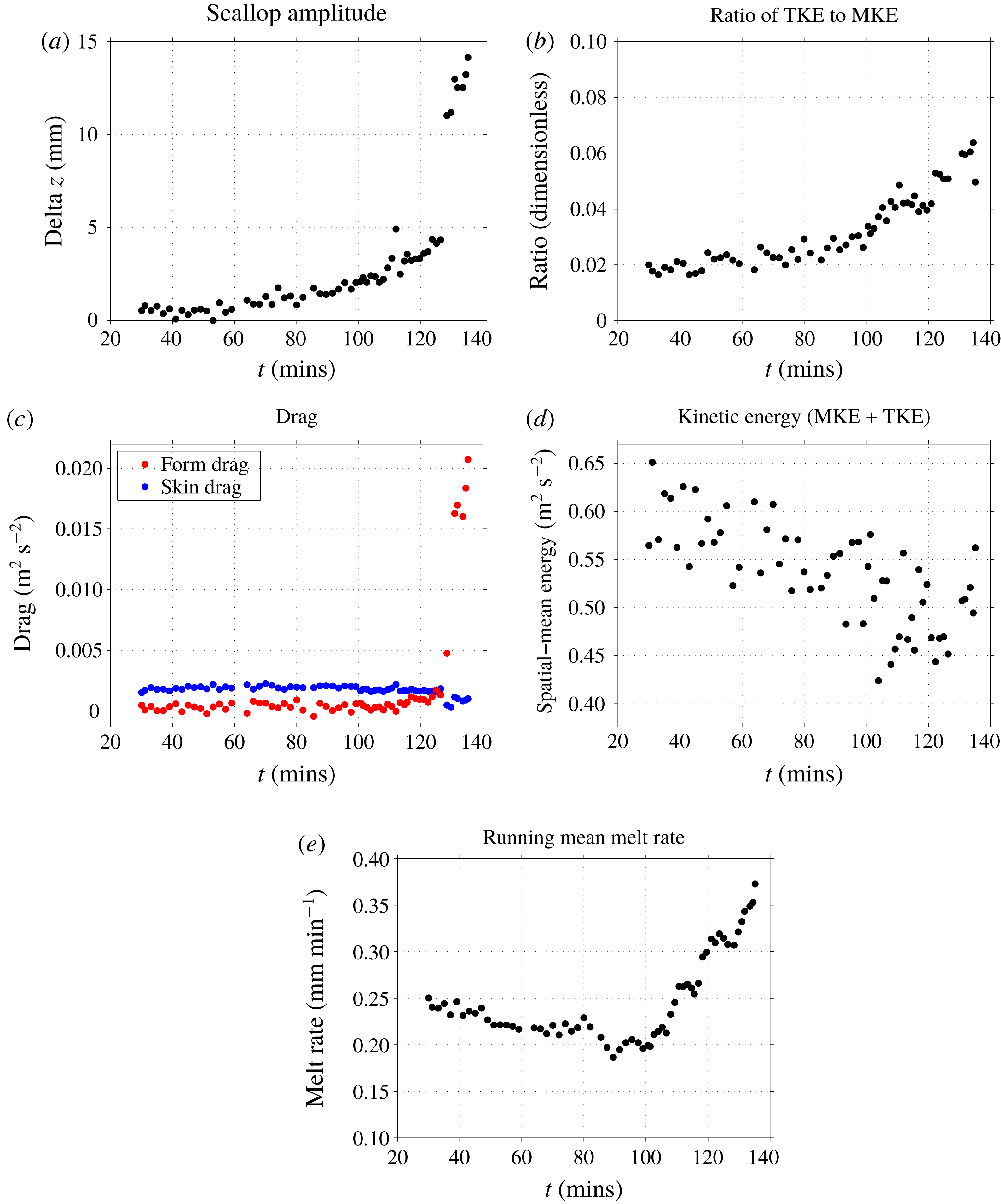
We have shown that scallops have a clear effect on the TKE of the ice–water boundary layer, tending to decelerate flow near the ice interface, suggesting a possible influence of scallops on fluid drag. We explore this next, considering the effect of an evolving ice–water geometry on form drag and skin drag. We let
 $z_{top}$
be the upper height limit of the data acquisition window and let
 $h(x,t)$
be the ice–water interface height. Integrating the momentum equation vertically between
 $h(x,t)$
and
 $z_{top}$
and horizontally between
 $x_{1}$
and
 $x_{2}$
, we obtain the mean form drag
 $F(t)$
as
 $$\begin{eqnarray}\displaystyle F(t)=\displaystyle {\displaystyle \frac{1}{{\mathcal{L}}}}\int _{x_{1}}^{x_{2}}{\displaystyle \frac{1}{\unicode[STIX]{x1D70C}}}{\displaystyle \frac{\unicode[STIX]{x2202}h(x,t)}{\unicode[STIX]{x2202}x}}p_{i}(x,t)\,\text{d}x, & & \displaystyle\end{eqnarray}$$
where
 $p_{i}(x,t)=p(x,z=h(x,t))$
is the pressure evaluated at the ice–water interface and
 ${\mathcal{L}}=x_{2}-x_{1}$
. We also recover the mean skin drag,
 $S(t)$
, defined as
 $$\begin{eqnarray}\displaystyle S(t)=\displaystyle -{\displaystyle \frac{1}{{\mathcal{L}}}}\int _{x_{1}}^{x_{2}}\!\int _{h(x,t)}^{z_{top}}\unicode[STIX]{x1D708}\unicode[STIX]{x1D6FB}^{2}u(x,z,t)\,\text{d}z\,\text{d}x. & & \displaystyle\end{eqnarray}$$
The skin drag is computed directly from the PIV-derived velocity fields. Note that, while these data do not resolve the curvature-free viscous sublayer, they do resolve the region of maximum curvature located near the transition between the buffer layer and the logarithmic layer, and therefore are able to provide a reliable estimate of the skin drag.
Pressure field (Pa) over flat ice (a), a developing scallop (b) and a fully developed scallop (c) from data collected in experiment 3.

Temporal evolutions of: (a) a scalloping ice geometry (defined as the difference between maximum and minimum interface height); (b) the ratio of turbulent kinetic energy to mean kinetic energy; (c) form drag and skin drag; (d) spatial-mean kinetic energy; and (e) running-mean melt rates. These data are from experiment 3.

We compute the form drag by applying the divergence theorem to the
 $x$
-component of
 $\unicode[STIX]{x1D735}\boldsymbol{\cdot }(p{\mathcal{I}})$
, where
 ${\mathcal{I}}$
is the identity matrix, which yields
 $\int _{V}(\unicode[STIX]{x2202}p/\unicode[STIX]{x2202}x)\,\text{d}V=\sum _{k}\int _{S_{k}}pn_{x}\,\text{d}S$
, where
 $V$
is the water portion of the domain and
 $n_{x}$
is the
 $x$
-component of the normal vector of the surface
 $S$
bounding the volume
 $V$
. The surface
 $S$
consists of four pieces:
 $S_{1}$
is the ice–water interface, which, after normalization by
 ${\mathcal{L}}$
and
 $\unicode[STIX]{x1D70C}$
, leads to the form drag expression in (4.9);
 $S_{3}$
is the horizontal upper surface, which has a vertical normal and does not contribute to the horizontal force; and the
 $S_{2}$
and
 $S_{4}$
contributions are vertical integrals computed over the left and right edges of the domain, respectively. We compute the form drag by directly computing
 $\int _{V}\unicode[STIX]{x2202}p/\unicode[STIX]{x2202}x$
and the surface integrals over
 $S_{2}$
and
 $S_{4}$
and applying the divergence theorem. This approach avoids having to evaluate the pressure field at the ice–water interface, which displays artifacts close to this boundary (see figure 12). Computing the form drag therefore requires a computation of the time-mean pressure field and pressure gradient for each 6.7 s data acquisition period. To compute the pressure field, we use the PIV-derived velocity fields to directly compute all other terms in (3.1). Taking the time mean of these terms yields a time-mean pressure gradient, which we integrate in
 $x$
to recover the pressure field. We perform these computations using a
 $\unicode[STIX]{x1D70E}$
vertical coordinate (see 4.2) in order to increase the robustness of horizontal integrals performed near the ice–water interface. The resulting pressure fields display artifacts of the
 $\unicode[STIX]{x1D70E}$
vertical coordinate, since errors along a constant-
 $\unicode[STIX]{x1D70E}$
surface accumulate as the horizontal integral is performed.
We find that, as the ice evolves from a flat to scalloped geometry, an adverse pressure gradient develops in the scallop trough, with low pressure anomalies on the leeward slope and high pressure anomalies on the streamward slope (see figure 12). This adverse pressure gradient acts to decelerate – or even reverse – the flow within the scallop trough, consistent with the recirculating mean flow shown in figure 5. The combination of low pressure on negative slopes and high pressure on positive slopes implies that there is a net form drag imparted on the flow as it traverses the scalloped geometry.
We now consider the temporal evolution of form drag and skin drag in experiment 3, in which the ice–water interface evolves from a flat to a scalloped geometry (see figure 13). Note that the first 55 samples in experiment 3 were collected at a fixed
 $x$
-position, and the measurement apparatus was moved to a more developed scallop for the final seven samples (see discontinuity in scallop amplitude in figure 13
a). We find that, as the ice becomes scalloped, the TKE near the ice–water interface increases (also see figure 9), whereas the total kinetic energy decreases, suggesting that the scalloped geometry is imparting a net drag on the flow. The TKE and mean kinetic energy (MKE) are computed as the average over all grid points within 24 mm of the ice–water interface. Over this time period, the skin drag values are relatively constant and decrease slightly as the ice becomes scalloped, consistent with the lower flow speeds in the scallop trough. Conversely, the form drag values sharply increase as the ice becomes scalloped, suggesting that changes in form drag are driving the observed decrease in total kinetic energy. This increased form drag suggests that, unlike the drag-minimizing effect of dimples on a golf ball (Achenbach Reference Achenbach1974), ice scallops are not a drag-minimizing phenomenon. Rather, scallops act to increase form drag, consistent with increased TKE and turbulent heat transfer near the ice–water interface. Indeed, we find that the running-mean melt rates (averaged over 15 interface profiles) show a general increase as the ice becomes scalloped (figure 13
e), implying that the ice geometry is enhancing turbulent heat and momentum transfer to the ice–water interface. This temporal evolution of ice geometry, TKE, form drag and melt rates is consistent with the scallop formation mechanism described in § 4.4.
5 Heat flux measurements
Heat flux measurements within a scallop trough from experiment 5. The dots are coloured and sized according to their magnitude. The black circles represent an uncertainty estimate of
 $\pm 1\unicode[STIX]{x1D70E}$
obtained via a bootstrap method. The black line is a spline interpolation of five measurements of the ice–water interface height (black dots), and represents an estimate of the ice-interface geometry.

To this point, we have evaluated the net effect of turbulent heat fluxes via ice-interface melt rates (§ 3), and have examined the velocity structure of the ice–water boundary layer in the presence of a scalloped-ice geometry (§ 4). Neither of these analyses is able to directly assess the spatial distribution of turbulent heat fluxes near a scalloped-ice surface. Here, we provide an assessment of the heat flux distribution near an equilibrium scallop geometry based on vertical heat flux measurements obtained in experiment 5 (see figure 14). We find that the measured heat fluxes within a scallop trough are broadly consistent with the scallop formation mechanism discussed in § 4.4. In particular, we find that the heat fluxes reach their minimum just downstream of the scallop crest and generally tend to increase with height above the interface. This pattern of heat fluxes is consistent with the observed equilibrium scallop melt rates in figure 3(d) and the scallop TKE distribution shown in figure 9(e). Owing to the fragility and frequency response of the fast thermistor, we were only able to obtain data within 10 mm of the ice–water interface, which limits our ability to make precise statements about the heat fluxes delivered to the ice–water interface. This result should be viewed with some caution, and future work is required to measure turbulent fluxes with improved spatial resolution near the ice–water interface for a variety of ice-interface geometries.
6 Effect of scallops on large-scale melt rate
A natural question relevant for ice–ocean modelling is whether scallops influence large-scale melt rates under sea ice, icebergs or ice shelves. In other words, should melt-rate parametrizations used in ice–ocean models be adjusted to account for ice geometric effects? In figure 15(a), we consider melt-rate data collected from all experiments performed in this study. We note that these experiments are conducted with fresh water and that melt rates could be modified in oceanic conditions with salt water and associated buoyancy-driven effects. We find that the observed melt rates scale roughly linearly with the free-stream velocity
 $U$
, consistent with the linear dependence on velocity in the commonly used three-equation melt-rate parametrization (Holland & Jenkins Reference Holland and Jenkins1999; Jenkins, Nicholls & Corr Reference Jenkins, Nicholls and Corr2010). Overall, we do not find a clear difference in melt rates between flat- and scalloped-ice surfaces across these experiments. It should be noted that most scallop data were collected with the crest positioned in the left portion of the image (e.g. see figure 5
b). This may introduce a sampling bias which underestimates scallop melt rates, since melt rates are systematically lower between the crest and the trough minimum position (see figure 3
d). Given this, we are unable to make a definitive statement on the impact of scallops on melt rates. This question requires future work, particularly using larger fields of view encompassing many scallop wavelengths.
(a) Spatial-mean melt rates versus free-stream velocity for all experimental data collected. Flat-ice geometry is indicated by dots, scalloped geometry is indicated by asterisks, and the case of an adjusting scallop is indicated by an open circle. The marker colours indicate the water temperature used for the experiments. All black markers have water temperatures of 0.6–1.0
 $^{\circ }$
C, blue markers have temperatures of 0.2
 $^{\circ }$
C, and red markers have temperatures above 1.0
 $^{\circ }$
C. (b) Scatterplot of observed melt rates versus parametrized melt rates (based on (6.1)). The parametrized melt rates are computed directly for each experiment using the free-stream velocity, water temperature and cold plate temperature. The black line is a line of slope 1 representing a match between parametrized and observed melt rates.

We can also use these melt-rate data as a comparison against existing melt-rate parametrizations. Specifically, we consider the three-equation parametrization of Holland & Jenkins (Reference Holland and Jenkins1999), which parametrizes the heat flux from water to ice as
 $$\begin{eqnarray}\displaystyle Q_{w}=\unicode[STIX]{x1D70C}_{w}c_{p,w}\unicode[STIX]{x1D6E4}u_{\ast }(T_{w}-T_{f}), & & \displaystyle\end{eqnarray}$$
where
 $\unicode[STIX]{x1D6E4}=1/[2.12\,\text{ln}(u_{\ast }\unicode[STIX]{x1D6FF}/\unicode[STIX]{x1D708})+12.5Pr^{2/3}-9]$
,
 $\unicode[STIX]{x1D6FF}$
is the thickness of the ice–water boundary layer and
 $Pr$
is the molecular Prandtl number. The friction velocity is typically parametrized via a quadratic drag law in which
 $u_{\ast }=\sqrt{C_{d}}U$
, where
 $C_{d}$
is a dimensionless drag coefficient. We compute heat flux estimates based on a commonly used
 $C_{d}$
value of
 $C_{d}=3\times 10^{-3}$
and
 $\unicode[STIX]{x1D6FF}=30\unicode[STIX]{x1D708}/u_{\ast }$
. Note that direct computations of
 $u_{\ast }$
reveal that
 $C_{d}$
varies strongly with ice geometry, with values (in units of
 $10^{-3}$
) of
 $1.4\pm 0.2$
,
 $2.3\pm 0.3$
and
 $2.3\pm 0.5$
for the flat, developing and developed scallop cases from experiment 3, respectively. These estimates are based on averages computed over the upper 10 mm of the domain and over ten, ten and seven datasets, respectively. This suggests that scalloped ice increases the drag coefficient, and that geometry-dependent drag coefficients may be necessary for future melt-rate parametrizations. For the present analysis, we use a constant
 $C_{d}$
value, as PIV data quality precludes direct computation of
 $u_{\ast }$
across all experiments. We estimate conductive heat fluxes at the ice–water interface by assuming a linear temperature gradient in the ice and using an ice thickness of 10 cm, and then compute ‘parametrized’ melt rates based on the difference between these fluxes. These melt rates are highly sensitive to the choice of drag coefficient and relatively insensitive to the ice thickness and ice–water boundary-layer thickness. We do not find a clear systematic difference between observed and parametrized melt rates; however, the large spread in observed melt rates makes this result rather inconclusive (figure 15
b). Our results suggest that melt parametrizations may underestimate high-melt regimes, but future additional experimental studies are required to properly answer this question.
7 Conclusions
In this work, we have investigated the mechanisms underlying the formation and maintenance of ice scallops, a small-scale ripple pattern that forms due to differential melting at the ice–water interface. We have performed a series of laboratory experiments in a refrigerated recirculating flume designed to probe the evolving ice–water boundary layer at high spatial and temporal resolutions. This work has demonstrated that particle image velocimetry (PIV) provides a viable experimental method for collecting high-quality sub-millimetre-scale velocity measurements in the ice–water boundary layer.
Under sufficiently high free-stream velocities (
 $U>0.6$
m s
 $^{-1}$
), we have found that scallops will form spontaneously from an initially flat ice–water interface. We have identified three distinct regimes of ice-interface evolution: (1) a scallop development regime in which melt rates are highest in scallop troughs, acting to amplify existing perturbations in the ice surface; (2) a scallop adjustment regime with highest melt rates over scallop crests, acting to dampen existing perturbations; and (3) an equilibrium scallop regime in which melt rates maintain a fixed scallop geometry which migrates downstream over time. The melt-rate profile of an equilibrium scallop geometry has a minimum occurring roughly one-quarter wavelength downstream of the crest and a maximum occurring roughly three-quarters of a wavelength downstream.
Our PIV-derived velocity data reveal that scallops are characterized by a time-mean recirculating eddy feature that exists within their troughs. This time-mean flow produces substantial modifications to the boundary-layer structure, with significantly reduced vertical shear near the ice–water interface and a far-field adjustment to a law-of-the-wall velocity profile. We have proposed a mechanism for scallop formation, in which scallops form due to a self-reinforcing feedback between the ice geometry and shear production of TKE in the flow interior. In this mechanism, the scallop crest position plays a crucial role, setting the location of high vertical shear of the mean horizontal flow and initiating a region of high shear production that extends to roughly the scallop trough minimum. This shear production creates TKE, which reaches a maximum value just downstream of the trough minimum, and produces maximum melt rates roughly three-quarters of a wavelength downstream of the crest. As the shear production reduces, the dominant source of TKE is lost, reducing the heat that is mixed down to the ice–water interface. This results in the ice interface rising up towards the next crest, re-establishing a zone of high vertical shear, and thereby creating a periodic flow feature that repeats in the subsequent scallop. Therefore, the length scale of this zone of high shear production is hypothesized to set the scallop wavelength.
We have found that, as an ice interface scallops, the form drag exerted on the flow tends to increase due to an adverse pressure gradient that develops in the scallop trough. This increased form drag also coincides with decreased total kinetic energy, increased turbulent kinetic energy and increased melt rates. Direct measurements of turbulent heat fluxes within a scallop trough show broad agreement with the flow features and melt rates obtained with PIV, with minimum heat fluxes occurring one-quarter wavelength downstream of the scallop crest.
This study provides a step towards a quantitative understanding of ice scallops, but a number of exciting open questions remain. In particular, we have identified that the length of the high shear production region is critical in setting the scallop wavelength, but have not explicitly addressed the physics that determine the length of this region and its dependence on Reynolds number. Secondly, this study has only considered a 2-D
 $x{-}z$
view of scallop flow. Future study is required to examine flow structures transverse to the mean flow and their role in setting the 3-D geometry of scallops. Moreover, future work is required to determine the net influence of scalloped geometry on large-scale melt rates, and to assess whether ice geometry should be factored into future ice–water heat flux model parametrizations. Finally, as scallops are commonly observed in the ocean, future laboratory experiments using salt water are needed in order to examine buoyancy-driven effects on ice-interface evolution. We hope that this study motivates future laboratory and numerical work on turbulence at the ice–water interface.
Acknowledgements
We thank three anonymous reviewers for constructive comments which improved the manuscript. This work is in part from the MELT project, a component of the International Thwaites Glacier Collaboration (ITGC) with support from the National Science Foundation (NSF-PLR 1739003) and Natural Environment Research Council (NE/S006656/1). ITGC Contrib. No. 001. We also acknowledge the support of NSF-EAGER 1144504, NSF-ARC 1304137, NASA-OMG NNX15AD55G and the NYU Abu Dhabi Center for Global Sea Level Change grant G1204. This work would not have been possible without the generous experimental assistance provided by the CRREL staff. We would particularly like to acknowledge the efforts of L. Zabilansky, G. Gooch, S. Bennet, D. Finnegan and A. LeWinter. We also thank M. Bae, D. Holland and B. Rougeux for their assistance in running and documenting the experiments. We thank C. Gladish and B. Wabah for many stimulating discussions on this work. We also thank B. Hobson and the Monterey Bay Aquarium Research Institute for sharing the scallop photos shown in figure 1(a,b).
Supplementary material
Supplementary material is available at https://doi.org/10.1017/jfm.2019.398.