


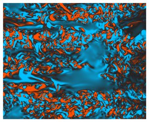


1. Introduction
Throughout much of the ocean interior, the spectrum  $\varPhi (k_z)$ of large-scale vertical shear (where
 $k_z$ is the vertical wavenumber) exhibits a strong degree of universality and is reasonably well approximated by the empirical Garrett–Munk (GM) spectrum (Garrett & Munk Reference Garrett and Munk1975). As reported by Gargett et al. (Reference Gargett, Hendricks, Sanford, Osborn and Williams1981) however, measurements from the upper ocean display a distinct steepening in the spectrum slope from
 $\varPhi \sim k_z^{0}$ (corresponding to the smallest scales in the GM spectrum) to
 $\varPhi \sim k_z^{-1}$ at scales of around
 $O(10\ \text {m})$, suggesting a change in the mechanisms leading to downscale energy transfer. At these scales, the influence of inertia becomes comparable to that of buoyancy, consistent with the conditions required for wave breaking, and the resulting turbulence might reasonably be expected to be influenced at leading order by stabilising buoyancy effects in the vertical direction. This regime can be formally defined in terms of a distinguished limit of dimensionless parameters in the governing equations and is often generically referred to as ‘strongly stratified turbulence’ (Lindborg Reference Lindborg2006; Brethouwer et al. Reference Brethouwer, Billant, Lindborg and Chomaz2007), though the geophysical relevance of this paradigm and its relationship to the internal wave field in the ocean has not yet been fully established. Considering a range of geophysical observations reported in the literature, Riley & Lindborg (Reference Riley and Lindborg2008) argue that the strongly stratified turbulence paradigm may be responsible for a number of observed atmospheric and oceanic spectra, with their arguments being furthered by Kunze (Reference Kunze2019) who suggests strongly stratified turbulence as a means of constructing a unified model for interpreting oceanic spectra. In any case, from both a geophysical and fluid dynamical perspective, many questions remain regarding the mechanisms producing small-scale vertical structure and turbulence, as well as the parameterisation of the resulting mixing.
For a uniformly stratified flow with horizontal length and velocity scales  $L$ and
 $U$, buoyancy frequency
 $N$, kinematic viscosity
 $\nu$ and density diffusivity
 $\kappa$, natural dimensionless parameters for characterising the evolution of the flow are the horizontal Reynolds number
 $Re_h$ and corresponding Froude number
 $Fr_h$ defined as
 \begin{equation} Re_h \equiv \frac{U L}{\nu},\quad Fr_h \equiv \frac{U }{NL }, \end{equation}
along with the molecular Prandtl number  $Pr\equiv \nu /\kappa$. If the flow is turbulent, an inertial range of scales with an isotropic energy cascade is expected in the horizontal, where now
 $U$ and
 $L$ represent the largest horizontal velocity and length scales injecting energy into turbulence. In the strongly stratified limit
 $Fr_h\ll 1$, buoyancy is expected to stabilise motions in the vertical direction and so, in addition to
 $Re_h\gg 1$, in order for fully isotropic (three-dimensional) turbulence to develop there must be a range of scales between the Ozmidov scale
 $L_O \sim (\varepsilon /N^3)^{1/2}$ characterising the largest vertical scales that are not influenced at leading order by the stratification and the Kolmogorov scale
 $L_K \sim (\nu ^3/\varepsilon )^{1/4}$, where
 $\varepsilon$ is the rate of dissipation of turbulent kinetic energy. This gives rise to the buoyancy Reynolds number
 \begin{equation} Re_b \equiv \frac{\varepsilon}{\nu N^2} \sim \left(\frac{L_O}{L_K}\right)^{4/3}. \end{equation}
The strongly stratified turbulent regime is generally associated with  $Fr_h\ll 1$,
 $Re_h \gg 1$ and
 $Re_b\gtrsim 1$. Note that, under the inertial scaling
 $\varepsilon \sim U^3/L$ we have
 $Re_b\sim Re_h Fr_h^2$, the latter often being used as an equivalent ‘turbulence intensity’ parameter in the flow (Brethouwer et al. Reference Brethouwer, Billant, Lindborg and Chomaz2007).
A notable flow feature associated with the strongly stratified limit is the formation of quasi-horizontal ‘pancake’ layers in the velocity and density fields with vertical extent  $L_v\sim U/N$ as predicted by the inviscid theory of Billant & Chomaz (Reference Billant and Chomaz2001), which has led to the regime sometimes being referred to as ‘layered anisotropic stratified turbulence’, or LAST, to more clearly differentiate the specific dynamics associated with this strongly stratified regime from inherently weakly stratified paradigms such as turbulence produced by Kelvin–Helmholtz instability (Falder, White & Caulfield Reference Falder, White and Caulfield2016; Caulfield Reference Caulfield2021). We will use this nomenclature subsequently. Below the scale of the largest vertical layers (denoted by the buoyancy scale
 $L_b \sim U/N$) and above the Ozmidov scale
 $L_O$, layering behaviour can be argued to exist on a scale-by-scale basis (i.e. smaller scale horizontal motions have smaller associated vertical length scales according to the stratified prediction) from which the spectrum of horizontal kinetic energy
 $E_h(k_z) \sim N^2k_z^{-3}$ for vertical wavenumber
 $k_z$ can be derived (Waite & Bartello Reference Waite and Bartello2004), in direct correspondence with the observed vertical shear spectrum
 $\varPhi \sim k_z^2E_h(k_z)\sim k_z^{-1}$. The
 $k_z^{-3}$ scaling has been notoriously elusive in studies using direct numerical simulation (DNS), though it is suggested that this may be due to contamination from smaller-scale near-isotropic vertical motions that are aliased into the associated buoyancy-inertial subrange due to the one-dimensional nature of the spectra (Almalkie & de Bruyn Kops Reference Almalkie and de Bruyn Kops2012; Augier, Chomaz & Billant Reference Augier, Chomaz and Billant2012; Maffioli Reference Maffioli2017; Howland, Taylor & Caulfield Reference Howland, Taylor and Caulfield2020).
Modelling flows in the LAST regime is difficult because of the large range of horizontal and vertical scales that must be resolved simultaneously, therefore, most existing studies are by DNS, although some features predicted by the theory have been recently observed in large-scale experiments (Rodda et al. Reference Rodda, Savaro, Davis, Reneuve, Augier, Sommeria, Valran, Viboud and Mordant2022). Many DNS provide a continual power input to turbulence through the use of a large-scale body forcing term added to the equations of motion, which are most commonly purely vortical, i.e. only modes with zero vertical wavenumber are forced (e.g. Waite & Bartello Reference Waite and Bartello2004; Brethouwer et al. Reference Brethouwer, Billant, Lindborg and Chomaz2007; Augier, Billant & Chomaz Reference Augier, Billant and Chomaz2015; Maffioli, Brethouwer & Lindborg Reference Maffioli, Brethouwer and Lindborg2016) or internal wave driven (e.g. Waite & Bartello Reference Waite and Bartello2006; Howland et al. Reference Howland, Taylor and Caulfield2020). In all cases a statistically stationary state is achieved by a forward cascade of energy through a sequence of instabilities that are, in general, not well understood, largely because the focus is on the properties of turbulence itself. Even in this idealised setting however, as demonstrated by Howland et al. (Reference Howland, Taylor and Caulfield2020), the energy pathways can vary significantly according to the large-scale mechanisms operating in the flow. Complicating matters further, some flows are observed to equilibrate in a state of relatively isolated ‘patches’ with distinct dynamical properties, as reported by Portwood et al. (Reference Portwood, de Bruyn Kops, Taylor, Salehipour and Caulfield2016).
Freely evolving stratified turbulent flows can be studied by DNS by imposing a stratification on top of initially homogeneous and isotropic velocity fields that subsequently decay, as originally studied by Riley, Metcalfe & Weissman (Reference Riley, Metcalfe and Weissman1981). These flows exhibit at least some of the same turbulence characteristics as forced stratified turbulence after a period of flow adjustment over approximately one buoyancy period  $2{\rm \pi} N^{-1}$ (de Bruyn Kops & Riley Reference de Bruyn Kops and Riley2019). The transient mechanisms required for a freely evolving flow to enter the LAST regime from a background quiescent state are less well studied. In the (necessarily) contrived spin-up period of forced flows, a layered structure can emerge from vortical forcing that is uniform in the vertical, often attributed to the ‘zigzag’ instability first observed by Billant & Chomaz (Reference Billant and Chomaz2000) in the form of decoupled vertical layers developing between two interacting stratified columnar vortices, which can produce regions of overturning and shear instability as natural precursors for turbulence (Deloncle, Billant & Chomaz Reference Deloncle, Billant and Chomaz2008; Waite & Smolarkiewicz Reference Waite and Smolarkiewicz2008; Augier & Billant Reference Augier and Billant2011). Without a body forcing however, turbulence is difficult both to initiate and maintain, as exemplified by the study of wall-forced flows that, to date, have only been shown to exhibit sustained fully developed turbulence for levels of stratification too weak to produce the required
 $Fr_h \ll 1$ (Deusebio, Caulfield & Taylor Reference Deusebio, Caulfield and Taylor2015; Zhou et al. Reference Zhou, Taylor, Caulfield and Linden2017; Lucas, Caulfield & Kerswell Reference Lucas, Caulfield and Kerswell2019).
Of course, as pointed out by Waite & Bartello (Reference Waite and Bartello2004) based on the observations of Polzin et al. (Reference Polzin, Kunze, Toole and Schmitt2003), vortical motions in the ocean are likely to coexist with the vertical structure due to the background internal wave field. An alternative argument for the existing vertical structure can be attributed to Gibson (Reference Gibson1987), who indicates that such variability could also be the result of ‘fossilised’ remnants of decaying turbulence occurring late during the evolution of a previous mixing event. Riley & de Bruyn Kops (Reference Riley and de Bruyn Kops2003) used a vertically varying idealised initial flow state consisting of idealised Taylor–Green vortices from which strongly stratified turbulence developed on top of layers of large vertical shear in the velocity fields. Motivated by the observations of Alford & Pinkel (Reference Alford and Pinkel2000), Howland, Taylor & Caulfield (Reference Howland, Taylor and Caulfield2021) demonstrate that the interaction of a background field of internal gravity waves with a layer of strong vertical shear can produce local regions of strong turbulence and mixing, which could perhaps in turn give rise to strongly stratified turbulence dynamics on larger scales. However, both of these studies assume an existing periodic vertical shear with fixed wavelength that is crucially of leading-order importance in the flow. Attempting to produce turbulence in the LAST regime under the relaxation of these conditions forms one of the main goals of this work.
A primary quantity of interest for parameterising small-scale mixing is its efficiency  $\eta$ measuring the rate of irreversible conversion of energy into the background potential energy of the flow (Gregg et al. Reference Gregg, D'Asaro, Riley and Kunze2018). Largely based on simulations of statistically stationary forced flows and decaying initially isotropic turbulence, the mixing properties of flows approaching the LAST regime, specifically the flux coefficient
 $\varGamma \equiv \eta /(1-\eta )$, have been argued to be primarily dependent on the parameter
 $Fr_h$ (Maffioli et al. Reference Maffioli, Brethouwer and Lindborg2016). Garanaik & Venayagamoorthy (Reference Garanaik and Venayagamoorthy2019) demonstrate that the ratio of the Ozmidov scale
 $L_O$ to the Thorpe scale
 $L_T$ measuring the size of the largest density overturns in the flow may be a reasonable proxy for the Froude number and, hence,
 $\varGamma$. This ratio has been used in transient vertical shear-driven mixing events as a measure of the ‘age’ of a turbulent mixing event, where, in this paradigm, early stage developing turbulence with
 $R_{OT}\ll 1$ is associated with large values of
 $\varGamma \gtrsim 1$ (Mashayek, Caulfield & Peltier Reference Mashayek, Caulfield and Peltier2017; Mashayek, Caulfield & Alford Reference Mashayek, Caulfield and Alford2021). It is not yet clear whether such values are obtainable in freely evolving flows that transition into the LAST regime. This is mainly due to a present lack of relevant DNS, though we note that, for sufficiently large Reynolds numbers, the data of Riley & de Bruyn Kops (Reference Riley and de Bruyn Kops2003) do demonstrate a significant early peak of
 $\varGamma \sim 0.7$ arising during the turbulent transition of their initial Taylor–Green vortex configuration.
Motivated by the above discussion, here we seek to demonstrate the existence of a novel transient pathway to LAST from a relatively generic yet physically plausible initial flow state, which importantly has relatively weak vertical shear. To do so, we consider the background flow studied by Basak & Sarkar (Reference Basak and Sarkar2006) (hereafter BS06) consisting of a horizontal shear layer in the presence of a uniform vertical density stratification, modified by adding perturbations to the horizontal velocity fields whose vertical structure consists of small-amplitude horizontal layers. This structure is motivated by (though not strictly representative of) the sort of vertical structure produced by a relatively weak background internal wave field with large horizontal to vertical aspect ratio, or by decaying turbulence from a previous mixing event. Crucially, the interaction of the initially weak vertical structure with the background vortical flow produces rapid transient growth of strong vertical shear layers via the lift-up mechanism of Ellingsen & Palm (Reference Ellingsen and Palm1975), which fundamentally alters the subsequent flow evolution and eventually facilitates a transition to fully developed turbulence. We study the properties of this turbulence, in particular its relevance to the strongly stratified turbulence paradigm, for a range of different appropriately defined initial Froude numbers  $Fr_0$ characterising the background flow, and discuss emerging patterns in the associated mixing properties.
The remainder of this paper is organised as follows. In § 2 we describe the DNS set-up, detailing the background flow and superposed small-amplitude perturbations, as well as outlining the theory behind the key lift-up mechanism that facilitates the early development of strong vertically sheared layers. The results from the DNS are presented in § 3, where we discuss both the early shear amplification and fully nonlinear stratified turbulent regime in detail, as well as analysing the properties of the resulting mixing. We conclude and discuss the implications of our results in the context of ocean mixing in § 4.
2. Set-up and theory
2.1. Ambient flow
As noted in the introduction, we consider the model background flow originally studied in BS06 consisting of a horizontal shear layer in the presence of uniform vertical density stratification. Denoting dimensional variables with a star, the corresponding one-dimensional background profiles for the streamwise velocity  $\overline {u^*}(y)$ and (total) density
 $\overline {\rho _t^*}(z)$ are given by
 \begin{equation} \overline{u^*}(y) = \Delta u^* \tanh\left(\frac{y^*}{h^*}\right)\!, \quad \overline{\rho^*_t}(z) = \rho_0^* - \Delta \rho^*\left(\frac{z^*}{h^*}\right)\!, \end{equation}
where  $h^*$ is half the shear layer thickness,
 $\Delta u^*$ is half of the velocity difference across the shear layer,
 $\Delta \rho ^*$ is half the density difference over an equivalent vertical distance and
 $\rho _0^* \gg \Delta \rho ^*$ is a reference density. In order to investigate the evolution of the profiles (2.1a,b) on a vertically periodic domain, we consider density perturbations
 $\rho ^*(\boldsymbol {x},t)$ away from the linear background state so that we can write
 $\rho _t^*(\boldsymbol {x},t) = \overline {\rho _t^*}(z) + \rho ^*(\boldsymbol {x},t).$ Defining non-dimensional variables
 \begin{align} t=t^*\Delta u^*/h^*, \quad \boldsymbol{x}=\boldsymbol{x}^*/h^*, \quad \boldsymbol{u} = \boldsymbol{u}^*/\Delta u^*, \quad \rho= \rho^*/\Delta\rho^*, \quad p=p^*/(\rho_0^*\Delta u^{*2}), \end{align}
the non-dimensional Boussinesq Navier–Stokes equations for the velocity field  $\boldsymbol {u}=(u,v,w)$, density perturbation
 $\rho$ and pressure perturbation
 $p$ (away from the hydrostatic pressure that balances the linear background density profile) are
 $$\begin{gather} \frac{\mathrm{D}{\boldsymbol{u}}}{\mathrm{D}t} =-\boldsymbol{\nabla} p -\left(\frac{1}{Fr_0^2}\right) \rho\hat{{\boldsymbol{z}}} +\frac{1}{Re_0}\nabla^2{\boldsymbol{u}}, \end{gather}$$
 $$\begin{gather}\boldsymbol{\nabla}\boldsymbol{\cdot}{\boldsymbol{u}} = 0, \end{gather}$$
 $$\begin{gather}\frac{\mathrm{D}\rho}{\mathrm{D}t} = w+ \frac{1}{Re_0Pr}\nabla^2\boldsymbol{\rho}. \end{gather}$$
The dimensionless Reynolds number  $Re_0$, Froude number
 $Fr_0$ and molecular Prandtl number
 $Pr$ are defined as
 \begin{equation} Re_0=\frac{\Delta u^* h^*}{\nu^*}, \quad Fr_0=\frac{\Delta u^*}{N_0^* h^*},\quad Pr=\frac{\nu^*}{\kappa^*}, \end{equation}
where  $g^*$ is the acceleration due to gravity,
 $\nu ^*$ is the kinematic viscosity,
 $\kappa ^*$ is the molecular density diffusivity, and the background buoyancy frequency
 $N_0^*(z)$ is defined by
 \begin{equation} N_0^{*2}(z) \equiv-\frac{g^*}{\rho_0^*}\frac{\partial \overline{\rho_t^*}}{\partial z^*} = \frac{g^*}{\rho_0^*}\frac{\Delta\rho^*}{h^*}. \end{equation}
Note that, for comparison with previous studies such as BS06, an equivalent ‘Richardson number’ can be defined as  $Ri_0 \equiv N_0^{*2}h^{*2}/\Delta u^{*2} =g^*\Delta \rho ^* h^*/(\rho _0^* \Delta u^{*2})$, so that
 $Ri_0=Fr_0^{-2}$. One advantage of using
 $Fr_0$ as opposed to
 $Ri_0$ is that it avoids potential confusion with the classical analogue problem consisting of a vertical rather than horizontal shear layer, where
 $Ri_0$ corresponds to the minimum gradient Richardson number in the centre of the shear layer and, thus, is a direct indicator of the susceptibility of the flow to Kelvin–Helmholtz instability for sufficiently small values of
 $Ri_0$.
As demonstrated by the linear stability analysis of Deloncle, Chomaz & Billant (Reference Deloncle, Chomaz and Billant2007), infinitesimal normal mode perturbations to this background flow have a fastest growing mode that is two dimensional with the vertical wavenumber  $k_z=0$, though for a sufficiently small initial Froude number
 $Fr_0$, vertical modes with
 $k_z\sim 1/Fr_0$ grow essentially as fast as the two-dimensional mode. The result is complex three-dimensional behaviour, with coherent Kelvin–Helmholtz billow structures emerging in the form of vertical columns that have significant defects over a vertical scale
 $L_v\sim U/N$, as observed in BS06. However, despite the flow organising into distinctive layers with large associated dissipation of kinetic and potential energy, the development of small-scale turbulence with corresponding buoyancy Reynolds number
 $Re_b\gtrsim 1$ from these layers is notably absent for sufficiently small
 $Fr_0$. Motivated by the existing vertical structure expected to be found in the ocean thermocline, here we propose an alternative (non-normal mode) mechanism for the expedited transition to small-scale turbulence whilst still maintaining small
 $Fr_0$.
2.2. Finite-amplitude perturbations and the lift-up mechanism
For an inviscid unstratified shear flow with initial velocity profile  $\boldsymbol {u}_{t=0}=\bar {u}(y)\hat {\boldsymbol {x}}$, small but finite-amplitude perturbations
 $[\tilde {u}, \tilde {v}, \tilde {w}, \tilde {p}](y,z,t=0)$ that are independent of the streamwise coordinate
 $x$ are subject to algebraic growth according to the lift-up mechanism originally proposed by Ellingsen & Palm (Reference Ellingsen and Palm1975). The linearised momentum equation for the total streamwise velocity
 $u$ is
 \begin{equation} \frac{\partial u}{\partial t} =-v\frac{\partial \bar{u}}{\partial y}, \end{equation}
and it can be argued using the linearised equation of motion for the streamwise vorticity  $\zeta _x =\partial w/\partial y - \partial v/\partial z$ that
 $v$ remains constant in time so that
 $u=u(0)-\tilde {v}t\partial \bar {u}/\partial y$ grows algebraically (a treatment of more general perturbations is given by Landahl Reference Landahl1980). The lift-up mechanism has since been proposed to be an important pathway to turbulent motion in a variety of viscous flows (e.g. Butler & Farrell Reference Butler and Farrell1992; Arratia, Caulfield & Chomaz Reference Arratia, Caulfield and Chomaz2013; Pickering et al. Reference Pickering, Rigas, Nogueira, Cavalieri, Schmidt and Colonius2020) and in viscous vertically sheared stratified flows (Kaminski, Caulfield & Taylor Reference Kaminski, Caulfield and Taylor2014, Reference Kaminski, Caulfield and Taylor2017). We will see that, for sufficiently large initial perturbations (though still small compared with the magnitude of the background flow velocity) in a vertically stratified yet horizontally sheared flow, the lift-up mechanism can act to amplify rapidly a horizontally uniform vertical layered structure in the streamwise velocity field that remains coherent due to the stabilising effect of stratification until horizontal shear instability causes the roll up of columnar Kelvin–Helmholtz billows.
We consider perturbations  $(\tilde {u}(z), \tilde {v}(z), 0)$ to the base flow described above in § 2.1, so that the initial velocity field can be written as
 \begin{equation} \boldsymbol{u}|_{t=0} = \bar{\boldsymbol{u}}(y) + \tilde{\boldsymbol{u}}(z) = \tanh(y)\hat{\boldsymbol{x}} + \tilde{u}(z)\hat{\boldsymbol{x}} + \tilde{v}(z)\hat{\boldsymbol{y}}. \end{equation}
The perturbations are designed to be representative of existing structures in the environment with a long horizontal wavelength (compared with the vertical wavelength, so that they are approximately independent of  $x$ and
 $y$), which subsequently encounter a region of high horizontal shear due to a background flow on scales much larger than the domain.
Similarly to Howland et al. (Reference Howland, Taylor and Caulfield2020) and Furue (Reference Furue2003), we define the perturbation velocities  $\tilde {u}(z)$ and
 $\tilde {v}(z)$ as a sum of shear modes
 $(A/k_z)\exp ({2{\rm \pi} {\rm i} k_z z/L_z +{\rm i}\phi })$, where
 $k_z$ is the vertical wavenumber taking positive integer values,
 $A$ is a constant amplitude and
 $\phi \in [0,2{\rm \pi} )$ is a random phase, giving a kinetic energy spectrum of
 $k_z^{-2}$ representative of the GM spectrum. We assume that this spectrum is pre-existent at large scales in our flow domain, summing shear modes over
 $k_z\leq 7$. In contrast to Howland et al. (Reference Howland, Taylor and Caulfield2020) however, the amplitude of the perturbation velocity field
 $\tilde {\boldsymbol {u}}$ is assumed to be relatively small compared with the background flow, though importantly are still finite amplitude. For the range of
 $Fr_0$ considered here, we will show that
 $|\tilde {\boldsymbol {u}}| \sim 0.01$ (compared with
 $|\bar {\boldsymbol {u}}|\sim 1$) results in horizontal layers in the streamwise velocity field
 $u$ that are transiently amplified and reach a similar magnitude to the initial background flow. Note that, for simplicity, the density field
 $\rho$ and the vertical velocity field
 $w$ remain unperturbed. The streamwise perturbations
 $\tilde {u}(z)$ are not strictly necessary for the lift-up mechanism to take place, but are included nonetheless to demonstrate that they do not inhibit the growth of the instability. We stress that the finite-amplitude perturbations we consider are by no means optimal in any mathematical sense, but we find they are sufficient for producing conditions that can induce a transition to energetic turbulence whilst maintaining a strong stratification in the sense that
 $Fr_h\ll 1$.
2.3. Numerical simulations
The equations of motion are solved in a channel domain  $(x,y,z) \in [0, L_x] \times [-L_y/2, L_y/2] \times [0,L_z]$ that is periodic in the vertical and streamwise
 $x$ directions. In the
 $y$ direction the boundary conditions at the walls
 $y=\pm L_y/2$ are free slip, no flux, i.e.
 $\partial \rho /\partial y = 0$ and
 $\partial \boldsymbol {u}/\partial y =\boldsymbol {0}$. The domain size in the streamwise direction
 $L_x=28.56$ is taken to be twice the wavelength of the most unstable two-dimensional mode of classical shear instability, whilst
 $L_z=L_x/2 = 14.28$ and
 $L_y=66.3$, which is sufficiently large such that the channel boundaries do not influence the flow in the centre of the domain. Direct numerical simulations are performed using Diablo (Taylor Reference Taylor2008), which treats periodic coordinate directions pseudo-spectrally with a 2/3 aliasing rule applied to the nonlinear terms and wall-bounded directions using a second-order finite-difference spatial discretisation. Time stepping is achieved using a third-order mixed implicit/explicit Runge–Kutta/Crank–Nicolson scheme. A stretched grid is used in the
 $y$ direction so that the spacing is finer in the centre of the shear layer
 $-12.5 \leq y \leq 12.5$ where small-scale turbulence occurs. To absorb internal waves that propagate through the stratification away from the centre of the shear layer, a sponge layer occupies the regions
 $-L_y/2 < y < -L_y/2 + 7$ and
 $L_y/2-7< y< L_y/2$, within which perturbations are quadratically damped to zero.
Since the dynamics are laminar before columnar billows start to develop, to speed up computation, this initial phase of each simulation is carried out at half the final full resolution in each coordinate direction, before, for flows in which fully three-dimensional turbulence subsequently develops, the velocity and density fields are upscaled onto the full resolution grid using Fourier resampling in the  $x$ and
 $z$ directions and linear interpolation in the
 $y$ direction. At this stage the flow is still laminar and only larger-scale motions are present so that any noise introduced by interpolation has little impact. The final resolution is sufficiently fine to ensure that
 $k_{max} L_k > 1$ throughout flow evolution, where
 $L_k = (Re_0^{-3}/\varepsilon )^{1/4}$ is the Kolmogorov length scale for domain-averaged turbulent kinetic energy dissipation
 $\varepsilon$, and
 $k_{max} = 2k_{nyq}/3$ is the maximum resolved wavenumber for Nyquist wavenumber
 $k_{nyq}={\rm \pi} N_x/L_x = {\rm \pi}N_z/L_z$ after dealiasing. Simulations are stopped around
 $30$ dimensionless time units after billow pairing takes place, as the dynamics after this become constrained artificially by the periodicity of the domain. The majority of the dynamics and turbulence we study below occurs either before or during pairing, giving us a good level of confidence that the domain size we use is sufficiently large.
Table 1 summarises the initial parameters and grid sizes for the DNS performed. We investigate the dynamics and evolution associated with the initial condition (2.9) for a range of initial Froude numbers  $Fr_0$. The same shape of the initial perturbation
 $\tilde {\boldsymbol {u}}$ is used for each simulation. To prescribe the amplitude
 $|\tilde {\boldsymbol {u}}|$, we observed that trial runs indicated perturbations
 $\boldsymbol {u'}$ to the background velocity field
 $\bar {\boldsymbol {u}}$ grew linearly with time with rate
 $|\tilde {v}|$ (so that
 $|\boldsymbol {u'}|\propto |\tilde {v}|t$ according to the lift-up mechanism, as detailed for the full DNS in § 3 below) before saturating in amplitude at a dimensionless time of approximately
 $4{\rm \pi} Fr_0$. We therefore select a target maximum amplitude
 $|\boldsymbol {u'}| = 0.2$ giving
 $|\tilde {\boldsymbol {u}}|= 0.2/(4{\rm \pi} Fr_0)$, hence determining a typical order of magnitude
 $|\tilde {\boldsymbol {u}}|\sim O(10^{-2})$ for the narrow range of
 $Fr_0\sim O(1)$ investigated here. The target amplitude of
 $|\boldsymbol {u'}|=0.2$ is the same for each simulation and is chosen so that the local gradient Richardson number
 \begin{equation} Ri_g(\boldsymbol{x},t)=\frac{1 -\partial\rho/\partial z }{Fr_0^2 |\partial \boldsymbol{u}/\partial z|^2} \end{equation}
remains above the marginal stability value of  $1/4$ at the interfaces between the layers that grow, preventing the onset of vertically stratified shear instability. For the sake of simplicity, and for arguably a better comparison with other DNS from the literature exhibiting LAST sustained by large-scale vortical motions, we focus on this limiting case where turbulent transition requires additional energy obtained from the onset and development of columnar vortices produced by horizontal shear instability, occurring once transient layer growth has taken place. The opposite limit, where the dynamics are dominated by the early development and breakdown of Kelvin–Helmholtz billows at the layer interfaces, has been well studied at least on the individual layer scale, and in the absence of the large-scale horizontal shear layer (see, e.g. the recent review by Caulfield Reference Caulfield2021).
Flow parameters and grid sizes for each DNS, where  $Ri_0$ is included for comparison with the DNS of BS06. Here
 $N_x$ and
 $N_z$ are the maximum number of grid points in the streamwise and vertical directions, respectively, whilst
 $N_y$ is the maximum number of grid points in the spanwise central region
 $-12.5\leq y \leq 12.5$. All simulations have
 $Pr=1$.

3. Results
3.1. Amplification of vertical shear
We begin by studying the transient growth of the initial state defined in (2.9) for the simulations F05, F1 and F2, where the results from simulation F07 follow a similar pattern and are omitted from this section for clarity. The initial perturbation  $(\tilde {u}(z), \tilde {v}(z),0)$ causes the magnitude of the streamwise velocity
 $u$ to increase rapidly before saturating at around
 $O(1)$, which we investigate in detail below. First, figure 1 shows visualisations of the streamwise velocity field
 $u$ at time
 $t\approx 48$ after saturation of the initial growth. Panel
 $(a)$ shows the vertical profile of the centreline velocity
 $u(0,0,z)$ for simulations F05 (red solid line), F1 (blue dashed line) and F2 (orange dot-dashed line). The black dotted line shows the shape of the initial perturbation
 $\tilde {v}(z)$ of the spanwise velocity normalised to have similar amplitude for ease of visualisation. A distinct vertical mode structure in
 $u$ is present, in all cases taking a similar (reflected) shape to the initial profile, which strongly suggests the growth in
 $u$ is locally determined by
 $\tilde {v}$ in a manner consistent with (2.8).
(a) Vertical profiles of streamwise velocity  $u(0,0,z)$ taken at time
 $t\approx 48$ for simulations F05 (red solid line), F1 (blue dashed line) and F2 (orange dot-dashed line). The black dotted line shows the shape of the initial spanwise velocity profile
 $\hat {\tilde {v}}(z)$ normalised to a similar amplitude for comparison. (b,c) Contour plots showing vertical slices from simulation F1 in the
 $y$ and
 $x$ planes of the streamwise velocity field (b)
 $u(x,0,z)$ and (c)
 $u(0,y,z)$. The directory including the data and Jupyter notebook for producing the figure can be found at https://multimediafluids.uam.elogim.com/S0022112024001216/JFM-Notebooks/files/fig1.

There are small but noticeable differences between the simulations with different initial Froude number  $Fr_0$: in general, a lower Froude number results in more pronounced higher wavenumber modes. Recalling that
 $\tilde {v}$ is constructed of a sum of randomly phased Fourier modes
 ${\rm e}^{{\rm i}mz}$ for the lowest seven permissible wavenumbers in the vertical, this means that the higher wavenumber modes exhibit enhanced growth for smaller
 $Fr_0$. This is entirely consistent with the results of Deloncle et al. (Reference Deloncle, Chomaz and Billant2007) who show that, for the same base flow without the additional vertical perturbations, three-dimensional infinitesimal normal mode perturbations with vertical wavenumber
 $m$ less than
 $1/Fr_0$ grow almost equally as fast as the most unstable two-dimensional mode with
 $m=0$ corresponding to that of classical unstratified shear instability, with a larger growth rate for smaller
 $Fr_0$. It is important to stress here that, though there exists a clear scaling similarity, the finite-amplitude modes we are considering here are entirely different and grow over a much shorter time scale than the infinitesimal perturbations considered by Deloncle et al. (Reference Deloncle, Chomaz and Billant2007), the latter of which can be seen emerging in the form of a vertical column defect length scale in the fully nonlinear simulations of BS06.
The quasi-steady state reached by the algebraic growth consists of horizontal layers in the streamwise velocity field that are localised at the velocity interface in the  $y$ direction and extend across the whole domain in the
 $x$ direction, as can be seen by looking at panels (b,c) of figure 1. We note that
 $v$,
 $w$ and
 $\rho$ are small in comparison to
 $u$ and only grow substantially once horizontal shear instability occurs later during the flow evolution. Panel (c) shows that the interface in the
 $y$ direction is distorted by the layering, though the magnitude of the maximum velocity gradient
 $\partial u/\partial y$ remains similar and, hence, as we will see, this distortion does not prevent the rolling up of the sheet of vorticity into Kelvin–Helmholtz billows in the
 $x$–
 $y$ plane caused by inflectional shear instability.
We now investigate the dynamics of the transient growth in detail. In figure 2 the centreline streamwise velocity magnitude  $\langle |u(y=0)|\rangle$ averaged over the
 $x$ and
 $z$ directions can be seen to increase linearly with time initially, matching the algebraic growth predicted by the lift-up mechanism of Ellingsen & Palm (Reference Ellingsen and Palm1975). Moreover, we can plot the corresponding
 $x$- and
 $z$-averaged terms from (2.8) to find a very good match with the predicted growth rate
 $\langle |v\partial \bar {u}/\partial y(y=0)|\rangle$. The streamwise velocity magnitude continues to grow until it starts to saturate at a time proportional to
 $Fr_0$, so that the saturation time for F1 is approximately double that of F05 and so on. Noting that the dimensionless buoyancy frequency is given by
 $1/Fr_0$, this indicates that the stratification is responsible for equilibrating the flow to a quasi-steady vertical layered state approximately over two buoyancy periods
 $4{\rm \pi} Fr_0$, which is then sustained until the growth of the horizontal shear instability becomes significant. Perhaps somewhat surprisingly, the agreement with (2.8) is maintained throughout the saturation of the layered state. This is because, as suggested by figure 1(b),
 $u$ and
 $p$ continue to remain independent of the streamwise coordinate
 $x$ as the perturbations grow. Meanwhile,
 $v$ decays and
 $w$ remains small, with the result being that the nonlinearities and pressure gradient term in the streamwise momentum equation are negligible (along with the viscous term) meaning it still reduces to the form (2.8).
The evolution of streamwise velocity magnitude evaluated at  $y=0$ and integrated over the
 $x$ and
 $z$ directions (right axis), as well as the corresponding terms in the linearised evolution equation (2.8) (left axis). Results are shown for simulations (a) F05, (c) F1 and (c) F2. The directory including the data and Jupyter notebook for producing the figure can be found at https://multimediafluids.uam.elogim.com/S0022112024001216/JFM-Notebooks/files/fig2.

It is worth briefly comparing the transient growth observed here to that seen in existing studies of the hyperbolic tangent shear layer profile. For the case of the unstratified shear layer (here obtained by taking  $Fr_0\to \infty$), Arratia et al. (Reference Arratia, Caulfield and Chomaz2013) show that infinitesimal perturbations of the form
 $\boldsymbol {u}_0(y) \exp ({{\rm i}k_xx+{\rm i}k_zz})$ optimizing the (linear) energy growth over sufficiently short time horizons are inherently three dimensional, i.e. both horizontal and vertical wavenumbers
 $k_x$ and
 $k_z$ are non-zero, in contrast to the classical most unstable two-dimensional shear instability mode with
 $k_z=0$ obtained from linear stability analysis. Kaminski et al. (Reference Kaminski, Caulfield and Taylor2014) find similar results for the stratified shear layer in the case where the shear is parallel to gravity (equivalent to gravity acting in the
 $y$ direction in the coordinate system we use here). In both studies, optimal perturbations over short time horizons consist of oblique waves localised at the centre of the shear layer and tilted against the shear, growing through a combination of the lift-up and Orr mechanisms (Orr Reference Orr1907; Farrell & Ioannou Reference Farrell and Ioannou1993), though the behaviour may be markedly different in the presence of stratification due to the excitation of internal gravity waves at some distance from the central interface. The inviscid linear evolution of non-normal perturbations to the initial condition (2.1a,b) used in this work where shear is orthogonal to gravity is studied by Arratia (Reference Arratia2011). This system is also discussed by Bakas & Farrell (Reference Bakas and Farrell2009a,Reference Bakas and Farrellb) as an extension of a more general investigation on the behaviour of internal wave perturbations on a flow with constant linear background shear. For the study here in which we focus primarily on the nonlinear flow evolution, it suffices to say that in both cases, optimal perturbations in the limit of
 $k_x \to 0$ exhibit linear streamwise velocity growth with time purely via the lift-up mechanism, precisely as we have observed here.
3.2. Turbulent transition
The initial conditions of BS06 are equivalent to ours in the absence of the vertical perturbations leading to horizontal layer formation. They observe the development of horizontal shear instability in the form of columnar vortices that interact with adjacent vortices over a characteristic vertical length scale dependent on  $Fr_0$. However, this length scale only becomes substantially smaller than the length scale of the horizontal shear mode for
 $Fr_0\lesssim 1$. Even when this is the case, the induced three-dimensional behaviour does not lead to a transition to small-scale turbulence. In our DNS, the lift-up mechanism enables the transient growth of layers with a significantly smaller vertical scale than the vertical length scale observed in BS06 associated with the fastest growing three-dimensional normal mode of the background flow. As discussed at the end of § 2.3, the magnitudes of vertical perturbations we impose on top of the set-up of BS06 are chosen so that the transient growth and saturation of the vertically sheared layers does not by itself destabilize the flow. Here we show that the subsequent onset of horizontal shear instability facilitates a transition to small-scale turbulence by interacting with the existing horizontal layers and enhancing the vertical shear between them, as well as creating local statically unstable overturns, or regions where the total density gradient
 $-1+ \partial \rho /\partial z >0$.
In figure 3 we use sequential violin plots (see the caption for a detailed description) to illustrate the evolution of the shape of the probability density function (p.d.f.) of the local gradient Richardson number  $Ri_g(x,0,z,t)$ defined in (2.10), evaluated in the plane
 $y=0$ at the centre of the horizontal shear layer. For clarity, only those values
 $-0.5< Ri_g<2$ are considered. At time
 $t=55$, the horizontal layers in
 $u$ have saturated in magnitude as is evident from figure 2. As per our design, the vertical shear at this point between the layers alone is not strong enough to trigger vertical shear instability and growing Kelvin–Helmholtz billows. This is reflected in the distributions of
 $Ri_g$, which do not exhibit values less than
 $1/4$ corresponding to the classical marginal stability value from the Miles–Howard criterion (though this is strictly only valid for normal mode perturbations to parallel inviscid stratified shear flows (Howard Reference Howard1961; Miles Reference Miles1961)) for any value of
 $Fr_0$.
Violin plots showing the evolution of the shape of the p.d.f. of the gradient Richardson number  $-0.5< Ri_g<2$ in the central plane
 $y=0$. Each plot is centred at its corresponding time on the
 $x$ axis. The breadth of the shaded region corresponds to the magnitude of the p.d.f. evaluated at the corresponding value of
 $Ri_g$ shown on the
 $y$ axis. Results are shown for simulations (a) F07, (b) F1 and (c) F2. The black dot-dashed lines correspond to the notional marginal value of
 $Ri_g=1/4$. Red lines (right axis) show the evolution of the spanwise perturbation velocity
 $\langle v'^2\rangle$ as an indicator for the onset of horizontal shear instability.

To trigger a transition to turbulence, the onset of horizontal shear instability is required. A proxy for the growth of this instability is the root-mean-square magnitude of the spanwise velocity  $\langle v^2\rangle$, here averaged over
 $y=0$, whose evolution is shown by the solid red lines in figure 3. Because the fastest growing mode of instability is purely horizontal (Deloncle et al. Reference Deloncle, Chomaz and Billant2007), the onset and development is not expected to be influenced strongly by
 $Fr_0$, as is consistent with the figure. However, the growing horizontal perturbation clearly interacts with and enhances the vertical shear between the existing layers, distinctly modifying both the shape and centre of the distribution of
 $Ri_g$. The effect is more pronounced for weaker stratification, or larger
 $Fr_0$. The growth of the horizontal mode results in the existence of local values of
 $Ri_g<1/4$ for all simulations, with an increasing relative density for smaller
 $Fr_0$. This indicates the potential for vertical shear instability (though we emphasise again that
 $Ri_g<1/4$ is only a notional, indicative proxy), which has often been assumed to be the canonical route to turbulence in LAST (e.g. Brethouwer et al. Reference Brethouwer, Billant, Lindborg and Chomaz2007). Moreover, values of
 $Ri_g<0$ corresponding to regions of static instability are observed, suggesting the advection of denser fluid over lighter fluid. One way this may be achieved is through the strong vertical shearing of horizontal gradients in density that arise due to the fact that the density perturbation field is strongly coupled to the vertical vorticity field, a feature that is discussed in detail in BS06.
In general, figure 3 illustrates how the growth of the horizontal shear mode renders the flow increasingly locally unstable and, hence, facilitates turbulent transition at small scales, provided  $Fr_0$ is not too small. As the trend in the distribution shape with
 $Fr_0$ suggests, for simulation F05, it was found that
 $Ri_g$ remains larger than
 $1/4$ everywhere even after the growth of the horizontal mode and, correspondingly, turbulence did not develop. This simulation is therefore excluded from the remainder of the discussion, where we focus on F07, F1 and F2. We stress that, by design, the existence of the horizontal layers formed by transient growth and the subsequent development of horizontal shear instability are both necessary for turbulent transition. In the absence of either, insufficient regions of vertical shear and static instability are generated for the development of small-scale instabilities. Though they are not considered here, it seems likely that initial perturbations with increasingly large amplitudes would eventually lead to local vertical shear instability dominating proceedings as discussed in § 2.3.
To illustrate the highly three-dimensional transition to turbulence fully, figures 4 and 5 show horizontal and vertical slices of the vertical vorticity field  $\zeta _z = \partial v/\partial x -\partial u/\partial y$ for simulations F07, F1 and F2 at various times throughout the flow evolution, following the initial development of horizontal layers. Despite the significant early growth of the horizontal layers described above, the subsequent flow still develops vertically coherent columnar billow structures due to horizontal shear instability in the manner described in BS06. This can clearly be seen in the left-hand panels of the two figures. Note that, in order to resolve small-scale turbulence, our simulations have a significantly smaller domain size in both the
 $x$ and
 $z$ directions than those of BS06 and, as a result, we do not see the billow interlocking behaviour they observe that occurs on vertical length scales close to the horizontal extent of the primary instability for
 $Fr_0=1$, though we note there is clear large-scale vertical decorrelation of billow pairing visible in figures 5(b) and 5(c) for the simulation F07 with the lowest
 $Fr_0$.
Horizontal planes  $z=0$ showing contours of the vertical vorticity field for simulations (a–c) F07, (d–f) F1, (g–i) F2. Plots (a,d,g) are taken at time
 $t=88$, (b,e,h) at
 $t=118$ and (c,f,i) at time
 $t=148$. Blue and red colours denote negative and positive values. An animated movie for simulation F1 is included in the supplementary materials available at https://doi.org/10.1017/jfm.2024.121. The directory including the data and Jupyter notebook for producing the figure can be found at https://multimediafluids.uam.elogim.com/S0022112024001216/JFM-Notebooks/files/fig4.

Similar to figure 4 but this time vertical planes  $y=0$ showing contours of the vertical vorticity field for simulations (a–c) F07, (d–f) F1, (g–i) F2. Plots (a,d,g) are taken at time
 $t=88$, (b,e,h) at
 $t=118$ and (c,f,i) at time
 $t=148$. Blue and red colours denote negative and positive values. An animated movie for simulation F1 is included in the supplementary materials. The directory including the data and Jupyter notebook for producing the figure can be found at https://multimediafluids.uam.elogim.com/S0022112024001216/JFM-Notebooks/files/fig5.

We observe distinctly different behaviour to that reported by BS06 occurring once columnar billows have formed, with the horizontal layers in the streamwise velocity field arising due to the lift-up mechanism strongly distorting the billow in the vertical at scales much smaller than its horizontal extent. This has the greatest effect on the outer regions, most notably the ‘braid’ structure that joins the two billows as can be seen in the left panels of figure 5. A breakdown to three-dimensional turbulence characterised by small-scale motions in the vorticity field follows the development of positive vertical vorticity structures in the braid seen in simulations F1 and F2, shown in figures 5(d) and 5(g). The braid vortex structures are not formed in flow F07, presumably due to the stronger influence of the stratification, though fully three-dimensional turbulence still eventually develops, as shown in panels (b,c).
At the same time, the enhancement of local vertical shear by the growing horizontal mode of instability means that the distributions of  $Ri_g$ shown in figure 3 for each simulation have an increased density of points with
 $Ri_g<1/4$. Moreover, the existence of horizontal gradients in density aligned with the structures in the vertical vorticity field in the presence of this vertical shear generates statically unstable regions with
 $Ri_g<0$ as discussed above. Thus, conditions are created consistent with both shear and convective instability leading to turbulence production. Based on the results of Parker et al. (Reference Parker, Howland, Caulfield and Kerswell2021) who study optimal perturbations on a breaking internal gravity wave through its interaction with a vertical shear layer, we think it reasonable to suppose here that the precise sequence of mechanisms leading to turbulence will depend on the energy available to growing perturbations from the time-evolving background flow, whose evolution itself is governed (at least) by the initial conditions and parameters
 $Re_0$,
 $Fr_0$ and
 $Pr$. This same complexity is also apparent during the breakdown of Kelvin–Helmholtz billows in a stratified shear layer, which develop a ‘zoo’ of secondary instabilities facilitating transition to small-scale turbulence that vary strongly with the strength of the background stratification, as well as
 $Re_0$ and
 $Pr$ (Mashayek & Peltier Reference Mashayek and Peltier2012a,Reference Mashayek and Peltierb; Salehipour, Peltier & Mashayek Reference Salehipour, Peltier and Mashayek2015).
The spatial locality of regions where turbulence is produced leads to obvious large-scale intermittency that is present in all simulations. Horizontal intermittency is mainly due to the coherent billow core structure, with both figures demonstrating the columnar vortices eventually pairing that is noticeably decorrelated at different heights for flows F07 and F1, as can be seen most clearly in figure 5(b). At these smaller values of  $Fr_0$, an increasing fraction of the vertical extent of the domain remains mostly laminar, likely due to the fact that the breakdown of the braid is inhibited by early pairing in these regions. Despite the differences in intermittency however, the centre and right-hand panels of figure 5 show that in general, where they are present, turbulent regions exhibit vertical anisotropy for all Froude numbers investigated, where emerging layered structures have a horizontal to vertical aspect ratio that increases with decreasing
 $Fr_0$. This is in qualitative agreement with the LAST regime.
3.3. Computation of turbulent statistics
Before exploring the dynamics of the three-dimensional flow regime quantitatively, we briefly outline how relevant statistics are calculated. Due to the presence of the initial background horizontal shear in the problem, the perturbation velocity field  $\boldsymbol {u}'(\boldsymbol {x},t)$ is defined in the same manner as in BS06 as the perturbation of the total velocity field
 $\boldsymbol {u}$ away from the ‘background profile’ obtained by averaging in the
 $x$ and
 $z$ directions:
 \begin{equation} \boldsymbol{u'}(\boldsymbol{x}, t) = \boldsymbol{u}(\boldsymbol{x},t) - \frac{1}{L_xL_z}\int_{x=0}^{L_x}\int_{z=0}^{L_z} \boldsymbol{u}\, {\rm d}\kern0.06em x\,{\rm d}z. \end{equation}
As seen above, the flows we are considering are transient and, especially at points early during turbulence development, highly spatially intermittent in both the vertical and horizontal directions. This makes computing representative bulk turbulent statistics challenging, since any box average will contain an a priori unknown volume fraction of quiescent regions. Perhaps the most obvious approach is to average statistics over a time-evolving three-dimensional turbulent region identified according to some threshold criterion on a field variable such as the turbulent kinetic energy, however the disk-space requirements for saving fully three-dimensional flow fields are too demanding to achieve a satisfactory resolution in time by this method. Since turbulence is generally centred on the location of the initial strip of vertical vorticity at  $y=0$, we suggest that a reasonable compromise for computing statistics is to consider vertical snapshots in the plane
 $y=0$ as illustrated in figure 5. Bulk statistics for the field variable
 $f(x,y,z,t)$ are then calculated by a plane average over the active turbulent region denoted by angle brackets
 $\langle {\cdot } \rangle _T$ with a subscript
 $T$,
 \begin{equation} \langle \,f(x,y,z) \rangle_T(t) = \frac{1}{L_x(L_z-z_{min})}\int_{x=0}^{L_x}\int_{z=z_{min}}^{L_z} f(x,0,z) \, {\rm d}\kern0.06em x\,{\rm d}z, \end{equation}
where  $z_{min}$ is chosen to neglect the largely quiescent lower regions in simulations F07 and F1. Specifically, we take
 $z_{min}=L_z/2 = 7.14$ for simulation F07,
 $z_{min}=4.0$ for simulation F1 and
 $z_{min} = 0$ for simulation F2. This approach removes the majority of the vertical intermittency and, on average, minimises the horizontal intermittency, though fluctuations in bulk values are expected as localised regions of turbulence are swept around the central part of the domain by the spinning and merging columnar billow structures seen in figure 4. The trade-off for a high time resolution is therefore that computed statistics are at best only broadly representative of flow behaviour. Nonetheless, we find that they prove to be sufficiently effective for characterising the key features of the flows we consider, as we show below. It is also worth pointing out the clear practical similarities between this problem and its observational analogue when dealing with experimental and field data: particularly relevant for the motivation of this study are oceanographic microstructure observations, for which the present most complete spatio-temporal datasets come from a chain of moored sensors (see, e.g. Ivey, Bluteau & Jones Reference Ivey, Bluteau and Jones2018).
3.4. Stratified turbulence characteristics
At least qualitatively, turbulence in all simulations exhibits behaviour that is consistent with the LAST regime. It is natural to ask whether this behaviour, despite arising in a highly spatially localised horizontal shear flow whose fully turbulent behaviour has not previously been considered, can be characterised by an appropriately defined set of turbulence parameters as discussed in the introduction. As argued by Zhou & Diamessis (Reference Zhou and Diamessis2019) and Portwood et al. (Reference Portwood, de Bruyn Kops, Taylor, Salehipour and Caulfield2016), since the flow we are considering is highly transient, it is perhaps most appropriate to define the horizontal Reynolds and Froude numbers  $Re_h$ and
 $Fr_h$ directly in terms of diagnosed energy-containing integral length scales
 $L$ and
 $L_v$ in the horizontal and vertical directions rather than indirectly appealing to the inertial scaling
 $\varepsilon \sim U^3/L$ often used in forced statistically stationary DNS (Brethouwer et al. Reference Brethouwer, Billant, Lindborg and Chomaz2007). To determine
 $L$ and
 $L_v$, we integrate the spectra of horizontal velocities in the plane
 $y=0$ using the method described in the appendix of Zhou & Diamessis (Reference Zhou and Diamessis2019). The results are shown in figure 6 for times
 $t>80$ following the onset of billow roll up. Figure 6(a) demonstrates that, despite the onset of turbulence,
 $L$ remains largely determined by the horizontal extent of the columnar billow structures throughout turbulent flow evolution. Billow pairing is clearly indicated by the rapid increase in
 $L$ (though the timing depends non-monotonically on
 $Fr_0$ due to the vertical decorrelation seen in figure 5). Consistent with the qualitative horizontal evolution shown in figure 4, this indicates that the horizontal kinetic energy and momentum balances are dominated by the emerging and interacting vortex columns. Looking at figure 6(b), the integral vertical scale
 $L_v$ is set by the layer growth that occurs prior to billow formation and notionally represents a dimensionless layer length scale. Despite some reasonable fluctuations (likely due to the manner in which it is calculated, as discussed above),
 $L_v$ maintains a similar magnitude over time, indicating that these layers are maintained throughout turbulence evolution. This behaviour of
 $L$ increasing whilst
 $L_v$ remains a similar magnitude is fairly typical of freely evolving flows in the LAST regime. In particular, we note the similarities with the freely evolving DNS of Riley & de Bruyn Kops (Reference Riley and de Bruyn Kops2003) initiated from a laminar Taylor–Green vortex configuration, which quickly develop strong horizontal vertically sheared layers that are maintained in structure and magnitude throughout the turbulent flow evolution despite the horizontal length scale increasing significantly. We define
 $Re_h$ and
 $Fr_h$ according to (1.1a,b), where the velocity scale
 $U=\mathcal {K}_h^{1/2}$ for
 $\mathcal {K}_h = \langle u'^2+v'^2\rangle _T/2$ and the average is taken as discussed above using (3.2). In dimensionless form we have
 \begin{equation} Re_h=Re_0 \mathcal{K}_h^{1/2} L, \quad Fr_h = \frac{Fr_0 \mathcal{K}_h^{1/2}}{L}. \end{equation}
The evolution of each turbulent flow in  $Re_h$-
 $Fr_h$ parameter space is shown in figure 7(a) by plotting
 $Re_h$ against
 $1/Fr_h$ as suggested by Brethouwer et al. (Reference Brethouwer, Billant, Lindborg and Chomaz2007), where their delineation of the ‘strongly stratified’ LAST regime according to
 $Fr_h<0.02$ and
 $Re_h Fr_h^{2}>1$ is shaded. According to our estimation of
 $Re_h$ and
 $Fr_h$, flows F1 and F07 can be seen in the figure to both narrowly fall within this regime during at least some of their evolution, whilst flow F2 remains only weakly affected by the stratification throughout. It is interesting to compare our results with Zhou & Diamessis (Reference Zhou and Diamessis2019), who, for a stratified turbulent wake behind a bluff body, derive a predicted turbulent Reynolds number
 $Re_h\sim Re_0Fr_0^{-2/3}$ based on the initial Reynolds and Froude numbers associated with the size of the body, using this to estimate empirically that strongly stratified turbulence is accessed when
 \begin{equation} Re_0 Fr_0^{-2/3} \gtrsim 5\times 10^3. \end{equation}
Evolution of the horizontal and vertical integral length scales (a)  $L$ and (b)
 $L_v$ for simulations F07 (blue lines), F1 (red lines) and F2 (orange lines). The directory including the data and Jupyter notebook for producing the figure can be found at https://multimediafluids.uam.elogim.com/S0022112024001216/JFM-Notebooks/files/fig6.

(a) Trajectories of  $Re_h$ vs
 $1/Fr_h$ for simulations F07, F1 and F2. The direction of time is from left to right, indicated by the grey arrow. Markers indicate the points at which the ‘fully turbulent’ snapshots considered in figures 8 and 9 are taken. The light blue shaded region denotes the ‘strongly stratified’ region of parameter space delineated by Brethouwer et al. (Reference Brethouwer, Billant, Lindborg and Chomaz2007) according to
 $Re_hFr_h^2>1$ and
 $Fr_h<0.02$. Panels (b,c) show the evolution of the buoyancy Reynolds number
 $Re_b$ and vertical Froude number
 $Fr_v$ for each simulation, where the dashed lines correspond to the time instant at which the markers are located in (a). The directory including the data and Jupyter notebook for producing the figure can be found at https://multimediafluids.uam.elogim.com/S0022112024001216/JFM-Notebooks/files/fig7.

Calculating a Reynolds and Froude number associated with the cylindrical billow structures that form with a diameter approximately  $L_x/2=14.28$ in our simulations as
 $Re_0^{{{{{\dagger}}}}} = 14.28 Re_0$ and
 $Fr_0^{{{{{\dagger}}}}} = Fr_0/14.28$, we find that
 $Re_0^{{{{{\dagger}}}}} Fr_0^{{{{{{\dagger}}}}} -2/3}\approx 6100$ for simulation F07R1,
 $Re_0^{{{{{\dagger}}}}} Fr_0^{{{{{{\dagger}}}}} -2/3}\approx 4900$ for F1R1 and
 $Re_0^{{{{{\dagger}}}}} Fr_0^{{{{{{\dagger}}}}} -2/3}\approx 3100$ for F2. This provides a perhaps fortuitously good match with the prediction of Zhou & Diamessis (Reference Zhou and Diamessis2019) despite the different flows under consideration, suggesting at least a non-trivial level of underlying similarity in the dynamics. Indeed, the derivation of their criterion essentially relies on the assumptions that turbulence parameters are primarily dependent on the large-scale properties of the flow on top of which turbulence develops, a feature that we also observe here.
We also define the buoyancy Reynolds number  $Re_b$ and the vertical Froude number
 $Fr_v$ (using the cyclic buoyancy period
 $2{\rm \pi} Fr_0$ as, for example, in the freely evolving flows of de Bruyn Kops & Riley Reference de Bruyn Kops and Riley2019; Zhou & Diamessis Reference Zhou and Diamessis2019) by
 \begin{equation} Re_b = Re_0 Fr_0^2 \varepsilon, \quad Fr_v = \frac{ 2{\rm \pi} Fr_0 \mathcal{K}_h^{1/2}}{L_v}, \end{equation}
where  $\varepsilon = \langle \partial _i u'_j\partial _i u'_j\rangle _T/Re_0$ is the dimensionless bulk turbulent kinetic energy dissipation rate. The time evolution of these quantities is shown in figure 7(b,c). Looking first at figure 7(b), both the maximum value of
 $Re_b$ and the time taken to reach this maximum depend strongly on the dimensionless buoyancy period
 $Fr_0$. In particular, just as with the prior development of the horizontal layers, the time taken for
 $Re_b$ to reach its first local maximum scales approximately linearly with
 $Fr_0$, demonstrating that turbulent transition is affected at leading order by the stratification. Once billow pairing has taken place,
 $Re_b$ starts to increase again for flows F1 and F2, likely due to the same mechanisms that caused the initial burst (though as discussed above, the simulations are stopped at this point as the dynamics start to become constrained by the periodicity). Peak values of
 $Re_b\approx 10$ and
 $Re_b\approx 5$ for the strongly stratified simulations F1 and F07 are high enough for the development of small-scale turbulent motions, though nonetheless imply at best a modest range of scales between the Ozmidov scale and the Kolmogorov length scale. Similar to the vertical length scale, the vertical Froude number plotted in figure 7(c) remains similar to its initial value determined by the shear layers that form prior to billow development and turbulence, and importantly, is
 $O(1)$ throughout turbulence evolution that is a characteristic signal of the stratified turbulence regime.
For each turbulent simulation, we look at a snapshot of the dissipation field  $\varepsilon$ when
 $Re_b$ is close to its peak value whilst
 $Fr_h$ is either less than
 $0.02$ (for flows F07 and F1) or as small as possible (for flow F2). The corresponding locations in parameter space are shown by the markers in figure 7(a) with times indicated by the dashed lines in panels (b,c). Vertical plane snapshots of the dissipation field are plotted in figure 8. Looking first at snapshots in the plane
 $x=0$ shown in the left panels, we can see that a range of small scales are present in all simulations, though remain highly localised to the central strip of vorticity associated with the initial horizontal shear flow that is distorted in the vertical by the vertically sheared layers that form. Horizontal layering of dissipation is obvious in simulations F07 and F1, while for the more weakly stratified flow F2, the distribution is more sparse. This is also clear from looking at the snapshots in the plane
 $y=0$ in the right panels where horizontally localised patches of turbulence are apparent in flow F2. We suggest that the reason for the differences between the spatial patterns in
 $\varepsilon$ is due to the timing of the development of turbulence, which depends strongly on
 $Fr_0$, relative to the evolution of the background horizontal flow set by the vortex columns, which is similar across all simulations. The results are consistent with a picture of turbulence onset being highly localised to unstable regions that are advected and extended by the background horizontal flow, matching the behaviour in the vertical vorticity field shown in figure 4. When
 $Fr_0$ is larger, turbulence develops rapidly and
 $Re_b$ is largest whilst the unstable regions are local to the outer regions of the billows causing the patchiness seen in figure 8(f). For smaller
 $Fr_0$, the time scale of turbulence development is large enough relative to that of the horizontal flow such that it is distributed throughout the domain by horizontal motions before decaying.
Vertical slices showing the dissipation field  $\varepsilon$, with (a,c,e) taken in the plane
 $x=0$ and (b,d,f) taken in the plane
 $y=0$. Plots (a,b) are from simulation F07, (c,d) from F1 and (e,f) from F2. For simulations F07 and F1 that are vertically intermittent, only the fully turbulent section of the vertical domain is shown. The snapshots are taken at times corresponding to the location of the markers in parameter space in figure 7(a), indicated explicitly by the dashed lines in 7(b,c). Note the logarithmic colour scale. The directory including the data and Jupyter notebook for producing the figure can be found at https://multimediafluids.uam.elogim.com/S0022112024001216/JFM-Notebooks/files/fig8.

Finally, we look at the one-dimensional horizontal and vertical spectra of horizontal kinetic energy for each simulation at the times corresponding to the markers in figure 7(a). Our pseudo-spectral DNS resolve discrete streamwise Fourier modes  $\exp ({\rm i}k_x)$ with wavenumbers
 $k_x=2{\rm \pi} n_x/L_x$ for integers
 $n_x$ between
 $0$ and
 $384$ (corresponding to the maximum wavenumber after dealiasing) and analagous vertical modes
 $\exp ({\rm i}k_z)$ with wavenumbers
 $k_z=2{\rm \pi} n_z/L_z$ for
 $n_z$ between
 $0$ and
 $170$. Spectra are calculated using the fully three-dimensional flow fields in the central turbulent region
 $-5< y<5$. Precisely,
 $$\begin{gather} E(k_x) = \frac{1}{2}\int_{y=-5}^{5}\left(\sum_{k_z}\hat{u}\hat{u}^* + \hat{v}\hat{v}^* \right) {\rm d}y, \end{gather}$$
 $$\begin{gather}E(k_z) = \frac{1}{2}\int_{y=-5}^{5}\left(\sum_{k_x}\hat{u}\hat{u}^* + \hat{v}\hat{v}^* \right) {\rm d}y, \end{gather}$$
where a hat denotes a Fourier transform in the  $x$ and
 $z$ directions and
 $*$ denotes complex conjugation.
Figure 9(a) demonstrates that, whilst  $Re_b$ is at, or close to, its maximum value, the horizontal spectrum for each simulation displays a plateau with a
 $k_x^{-5/3}$ slope indicating an incipient inertial range in the horizontal scales that is consistent with other vortically forced simulations at similar
 $Re_b$ by, e.g. Howland et al. (Reference Howland, Taylor and Caulfield2020), Augier et al. (Reference Augier, Billant and Chomaz2015) and Lindborg (Reference Lindborg2006). For sufficiently small
 $Fr_h$, the buoyancy wavenumber
 $k_b = (Fr_0 \mathcal {K}^{1/2})^{-1}$ becomes a dynamically relevant parameter (Billant & Chomaz Reference Billant and Chomaz2001) that, under the fundamental assumption that the vertical Froude number
 $Fr_v$ defined in (3.5a,b) is
 $O(1)$, scales with the wavenumber
 $2{\rm \pi} /L_v$ corresponding to the integral vertical scale
 $L_v$ set by the initial layers that form. The latter is easily recognisable as the location of the distinctive sharp peaks visible in figure 9(b). To draw attention to dynamics at scales influenced strongly by buoyancy, it is revealing to plot the vertical spectra as a function of the vertical wavenumber normalised by the Ozmidov wavenumber
 \begin{equation} k_O \equiv (Fr_0^{-3}/\varepsilon)^{1/2}. \end{equation}
In the LAST regime a range of anisotropic scales is expected to emerge between  $k_b$ and
 $m_O$ where
 $E(k_z)\sim k_z^{-3}$, followed at wavenumbers larger than
 $k_O$ by an increase in gradient towards the isotropic slope
 $k_z^{-5/3}$ provided that
 $Re_b$ is sufficiently large, that is, there is a range of turbulent scales between
 $k_O$ and the Kolmogorov wavenumber
 $k_K = (Re_0^{-3}/\varepsilon )^{-1/4}$ that do not feel the influence of the stratification. In all of our simulations there are at most a few decades of scales within the entire range
 $k_b< k_O< k_K$ so it is not surprising that these subranges are not distinct in figure 9(b). However, clearly the range of wavenumbers between
 $k_O$ and the wavenumber of the vertical layers that form corresponding to the sharp peaks increases with decreasing
 $Fr_0$. For the lowest
 $Fr_0=0.71$, a hint of an
 $k_z^{-3}$ plateau emerges, which is consistent with being at least marginally inside the strongly stratified turbulent regime. As suggested by Almalkie & de Bruyn Kops (Reference Almalkie and de Bruyn Kops2012) and explored in detail by Maffioli (Reference Maffioli2017) and Howland et al. (Reference Howland, Taylor and Caulfield2020), due to the natural spatial variation in the vertical length scales associated with a given horizontal scale, the use of one-dimensional spectra results in the aliasing of some of the energy contained in small-scale horizontal motions onto relatively low vertical wavenumbers that acts to obscure the narrow
 $k_z^{-3}$ plateau at low to moderate values of
 $Re_b$.
(a) Compensated horizontal (streamwise) spectra of kinetic energy  $k_x^{5/3} E(k_x)$; (b) compensated vertical spectra of kinetic energy
 $k_z^3 E(k_z)$; (c) vertical spectra of kinetic energy as in (b), where this time the sum is taken over streamwise modes
 $k_x>0$. Lines are coloured consistent with the previous figures. Spectra are evaluated using the full three-dimensional flow fields. The directory including the data and Jupyter notebook for producing the figure can be found at https://multimediafluids.uam.elogim.com/S0022112024001216/JFM-Notebooks/files/fig9.

We can remove the low wavenumber peaks in the vertical spectra by noting that the shear layers that cause them extend horizontally across the entire domain. Therefore, by computing the power spectral density whilst taking the sum in (3.7) over  $k_x\neq 0$, we can isolate the dynamics in the absence of the these largest-scale horizontal motions. The results are shown in figure 9(c), which somewhat more convincingly demonstrates the tendency of the vertical spectra towards an
 $k_z^{-3}$ plateau as
 $Fr_h$ decreases, suggesting the emergence of the associated buoyancy-inertial range. Additionally, as
 $Re_b$ increases from simulation F07 to simulation F2, the compensated spectra exhibit persistently steeper slopes towards vertical wavenumbers larger than
 $k_O$, displaying a plausible tendency towards the existence of an inertial range whose slope is indicated by the dashed line. In general, comparing the three spectra demonstrates a clear transition from the behaviour of stratified turbulence containing wavenumbers mostly smaller than
 $k_O$ (simulation F07) to that containing wavenumbers mostly at or larger than
 $k_O$ (simulation F2), whilst the overlap in the buoyancy and inertial subranges at wavenumbers close to
 $k_O$ highlights the difficulty in performing DNS with a large enough dynamic range to resolve both simultaneously. As of yet, DNS have not been able to reveal distinctly both the proposed isotropic and buoyancy-inertial vertical wavenumber range in stratified turbulence due to present computational limitations. Nonetheless, despite the time-dependent nature of the flow we are considering, the results here are at least suggestive that our DNS can transiently access a regime whose corresponding spectra behave in a manner consistent with arguably the most closely matching vortically forced flows of Maffioli (Reference Maffioli2017).
3.5. Mixing
We assume the irreversible mixing rate to be equivalent to the rate of destruction of buoyancy variance  $\chi$ defined for density perturbations
 $\rho$ from a uniform background density gradient as
 \begin{equation} \chi = \frac{1}{Re_0 Pr Fr_0^2} \langle \partial_i \rho\partial_i\rho\rangle_T . \end{equation}
Technically, a precise definition describing the evolution of the potential energy associated with an appropriate background density profile as proposed by Winters & D'Asaro (Reference Winters and D'Asaro1996) should be invoked, however, the practical difficulties in implementing this method and the feasibility of direct measurements of  $\chi$ in the ocean have led to (3.9) being regularly taken to be the definition of the mixing rate. Howland et al. (Reference Howland, Taylor and Caulfield2021) show that
 $\chi$ as defined above remains within 10 % of the ‘true’ mixing rate in a variety of forced stratified turbulent flows, with similarly good agreements being found for freely evolving vertically sheared flows (Lewin & Caulfield Reference Lewin and Caulfield2021).
An associated mixing efficiency  $\eta$ and flux coefficient
 $\varGamma$ can be defined instantaneously or cumulatively (denoted with subscripts ‘i’ and ‘c’, respectively) as
 $$\begin{gather} \eta_i(t) = \frac{\chi}{\chi + \varepsilon}, \quad \varGamma_i(t) = \frac{\chi}{\varepsilon}; \end{gather}$$
 $$\begin{gather}\eta_c(t) = \frac{\displaystyle\int\nolimits_0^t \chi \,{\rm d}t}{\displaystyle\int\nolimits_0^t (\chi+\varepsilon)\, {\rm d}t}, \quad \varGamma_c(t) = \frac{\displaystyle\int\nolimits_0^t \chi \,{\rm d}t}{ \displaystyle\int\nolimits_0^t \varepsilon\, {\rm d}t}. \end{gather}$$
Note that  $\eta = \varGamma /(1+\varGamma )$ in both the instantaneous and cumulative sense. Plots of
 $\chi$ and the associated dissipation
 $\varepsilon$ are shown in figure 10(a). The behaviour of
 $\varepsilon$ was previously discussed in the form of
 $Re_b= Re_0 Fr_0^{2}\varepsilon$, but is included as the dashed lines to facilitate a direct comparison with
 $\chi$ in the context of mixing. There is a notable similarity in the early behaviour of both
 $\chi$ and
 $\varepsilon$ in simulations F1 and F2, with both quantities increasing almost immediately following the formation of columnar billows. The onset of growth for simulation F07 is substantially more delayed. This may be attributed to the vortex structures that form in the braid region early during flow evolution for flows F1 and F2 but not for the more strongly stratified F07, as discussed in § 3.2. Corresponding behaviour is also marked in the plots of
 $\varGamma _i$ and
 $\varGamma _c$ shown in figure 10(b), where values early during turbulence development are similar for flows F1 and F2 and significantly larger than those of F07, representing larger mixing efficiencies during this stage. Indeed, the difference in the late-stage values of cumulative
 $\varGamma _c$ between flows F07 and F1 is likely due to this early behaviour. The pattern of larger values of the mixing efficiency being linked to coherent small-scale structures formed prior to turbulent transition has an analogue for the stratified vertical shear layer problem demonstrated by Mashayek, Caulfield & Peltier (Reference Mashayek, Caulfield and Peltier2013) and Lewin & Caulfield (Reference Lewin and Caulfield2021) in the context of coherent secondary shear instabilities that develop on the periphery of the (vertical) Kelvin–Helmholtz billow structures that form.
Time evolution of (a)  $\chi$ (solid lines) with
 $\varepsilon$ (dashed lines) superposed; (b) instantaneous and cumulative flux coefficients
 $\varGamma _i$ (solid lines) and
 $\varGamma _c$ (dotted lines). Each simulation is indicated by the colours consistent with previous figures. The directory including the data and Jupyter notebook for producing the figure can be found at https://multimediafluids.uam.elogim.com/S0022112024001216/JFM-Notebooks/files/fig10.

The behaviour of  $\chi$ later during flow evolution closely follows that of
 $\varepsilon$, peaking at around the same time for each flow. However, the associated ratio
 $\varGamma _i$ adjusts once turbulence develops so that flows F07 and F1 match very closely with values of
 $\varGamma _i$ between
 $0.3$ and
 $0.4$, whilst flow F2 displays larger values of
 $\varGamma _i$ between
 $0.4$ and
 $0.5$. This is consistent with the results of Maffioli et al. (Reference Maffioli, Brethouwer and Lindborg2016), who find that, for stratified turbulent flows maintained by vortical forcing, an appropriately defined
 $\varGamma$ appears to exhibit a maximum value of around
 $0.5$ at moderate values of
 $Fr_h\approx 0.3$ before decreasing and eventually tending towards a constant value of
 $\varGamma \approx 0.35$ as
 $Fr_h$ decreases towards around
 $O(10^{-2})$. Based on the results from the previous section, the point at which
 $\varGamma _i$ becomes roughly equal to this asymptotic value (or rather, for our transient flows, the point at which
 $\varGamma _i$ settles on the same trajectory for flows F07 and F1) appears to be determined by the entrance of the flow into the LAST regime, controlled by
 $Fr_h$. The physical reason for this has been argued through the consideration of the dominant scaling balances in this regime, for example, by Maffioli et al. (Reference Maffioli, Brethouwer and Lindborg2016) and Garanaik & Venayagamoorthy (Reference Garanaik and Venayagamoorthy2019). Our values of
 $\varGamma _i$ and their dependence on
 $Fr_h$ are consistent with simulations forced with vertically uniform large-scale vortical modes reported by both Howland et al. (Reference Howland, Taylor and Caulfield2020) and Maffioli et al. (Reference Maffioli, Brethouwer and Lindborg2016). Values of (an appropriately defined)
 $\varGamma \approx 0.4$ were also reported in stratified turbulence resulting from the freely evolving Taylor–Green vortex configuration of Riley & de Bruyn Kops (Reference Riley and de Bruyn Kops2003), as well as in the simulations of Jacobitz & Sarkar (Reference Jacobitz and Sarkar2000) forced with uniform horizontal shear.
3.6. Length scales
Motivated by the recent developments in analysing the relationship between important dynamical length scales in the flow, we define the Ozmidov scale  $L_O=2{\rm \pi} /k_O$, where
 $k_O$ is given by (3.8), as well as the Thorpe scale
 $L_T$ as the root-mean-square displacement of fluid parcels in each individual vertical column from their height in the corresponding profile that is sorted so that density monotonically decreases with depth. Precisely,
 $L_T=\sqrt {\langle \delta _T^2\rangle _T }$, where
 $\delta _T(\boldsymbol {x},t) = z(\rho ^*(\boldsymbol {x},t)) - z(\rho (\boldsymbol {x},t))$ is the displacement of a parcel at position
 $z(\rho ^*(\boldsymbol {x},t))$ in the sorted density field
 $\rho ^*(\boldsymbol {x},t)$ (obtained by rearranging the values of
 $\rho$ in each vertical column to be monotonically increasing with depth) from its position in the observed density field
 $z(\rho (\boldsymbol {x},t))$. The ratio of Ozmidov to Thorpe scales
 $R_{OT} = L_O/L_T$ has been proposed by Dillon (Reference Dillon1982) as a measure of the age of a turbulent event in the context of vertical shear-driven mixing as discussed in Smyth, Moum & Caldwell (Reference Smyth, Moum and Caldwell2001) and more recently, for example, in Lewin & Caulfield (Reference Lewin and Caulfield2021), with values of
 $R_{OT}\ll 1$ associated with early stage turbulence with larger corresponding
 $\varGamma$ and values
 $R_{OT}\gg 1$ with late-stage decay where
 $\varGamma \to 0$. For strongly stratified turbulence, Garanaik & Venayagamoorthy (Reference Garanaik and Venayagamoorthy2019) argue (using the Ellison scale discussed in Lewin & Caulfield (Reference Lewin and Caulfield2021) as a substitute for the Thorpe scale) that
 $R_{OT}$ may be a reasonable proxy for the Froude number
 $Fr_h$, though without considering developing turbulence do not cover values of
 $R_{OT}\ll 1$. They find
 $\varGamma$ roughly tends to a constant of
 $O(1)$ for
 $R_{OT}\sim 1$. Since our simulations contain both a period of young turbulence, and later of strongly stratified turbulence, we can investigate whether or not a corresponding signal exists in
 $R_{OT}$ for each of these stages.
The solid lines in figure 11(a) show the time evolution of  $R_{OT}$ for each simulation. In general, for our simulations,
 $R_{OT}$ remains
 $O(1)$ throughout the mixing event that is broadly consistent with Garanaik & Venayagamoorthy (Reference Garanaik and Venayagamoorthy2019) who predict that
 $\varGamma$ should remain roughly constant at around
 $O(1)$ in this regime. Actually
 $R_{OT}\sim 1$ also corresponds to the optimal ‘Goldilocks mixing’ regime of Mashayek et al. (Reference Mashayek, Caulfield and Alford2021) within which
 $\varGamma \sim O(1)$. Though this is derived within the setting of mixing by Kelvin–Helmholtz instability, which is in principle entirely different to the LAST regime, we point towards the possibility of the Kelvin–Helmholtz instability paradigm existing locally at scales below the buoyancy scale set by the vertically sheared layers within LAST. All flows studied here follow a pattern of
 $R_{OT}$ being smaller during transition and then increasing once turbulence is fully developed, which is at least consistent with the ‘young’ turbulence picture of Mashayek et al. (Reference Mashayek, Caulfield and Peltier2017, Reference Mashayek, Caulfield and Alford2021), though we do not observe
 $R_{OT}\ll 1$ as would be needed to fully verify this picture. This is perhaps unsurprising as such a regime would normally be associated with values of
 $\varGamma \geq 1$ not seen here. Whether or not there are mechanisms by which strongly stratified flows can produce local overturns with much larger scale than the global Ozmidov scale
 $L_O$ and, therefore, access a regime with
 $R_{OT}\ll 1$ and
 $\varGamma \gtrsim 1$ remains an open question.
(a) Time evolution of the ratio  $R_{OT}=L_O/L_T$ of Ozmidov to Thorpe scales (solid lines, left axis), where the corresponding shaded regions (right axis) represent the fraction of the domain that has a Thorpe displacement
 $\delta _T>0$. Lines are coloured as in previous figures. (b) Plots of the p.d.f. of
 $\log _{10}\varepsilon$ over the turbulent domain at times corresponding to the markers in figure 7, also indicated by the dashed lines in panel (a). The directory including the data and Jupyter notebook for producing the figure can be found at https://multimediafluids.uam.elogim.com/S0022112024001216/JFM-Notebooks/files/fig11.

An alternative, though closely related, view comes considering the fraction of the domain that is statically unstable, or equivalently, has  $|\delta _T|>0$. This is represented by the background shaded regions colour matched to the lines in figure 11(a). The behaviour is as expected, with the fraction of overturning increasing with increasing
 $Fr_0$. Flow F2 peaks at around
 $50\,\%$ overturning fraction, F1 around
 $35\,\%$ and F07 at just under
 $25\,\%$. In their classification of dynamically distinct regions in forced stratified turbulence, Portwood et al. (Reference Portwood, de Bruyn Kops, Taylor, Salehipour and Caulfield2016) determine turbulent patches as having an overturning fraction greater than
 $35\,\%$, layers as having a fraction between
 $20\,\%$ and
 $30\,\%$ and quiescent regions as having less than
 $20\,\%$. This roughly classifies F2 as a turbulent patch and F1 and F07 as layers, which is consistent with the entering of the latter two into the LAST regime accompanied by a change in the mixing properties. We have not investigated whether or not the turbulence we are considering in each simulation can be further subdivided into smaller patches with dynamically distinct signatures, which would require a careful filtering procedure. However, figure 11(b) offers some evidence that, at least when turbulence is fully developed, this is not necessary for our purposes. Plotted are the p.d.f.s (equivalent to normalised frequency distributions) of
 $\log _{10}(\varepsilon )$ over the domain at the time indicated by the vertical dashed lines in panel (a). We note that they are close to log-normal as expected for stratified turbulent flows with a sufficiently broad inertial range (de Bruyn Kops Reference de Bruyn Kops2015), and in particular, lack the right ‘shoulder’ feature that was a characteristic signature of high
 $Re_b$ patches in the flows studied by Portwood et al. (Reference Portwood, de Bruyn Kops, Taylor, Salehipour and Caulfield2016) (though flows F07 and F2 exhibit slight shoulders on the left of the distribution indicating the possible presence of small quiescent regions).
4. Discussion and conclusions
Much of the strongly stratified turbulence literature has focused on flows where turbulence is maintained in a statistically stationary state by large-scale body forcing. Removing time dependence from the problem simplifies the process of understanding the flow in terms of a set of suitably defined turbulence parameters, though there still appears to be significant variation in the way these flows are organised spatially (Portwood et al. Reference Portwood, de Bruyn Kops, Taylor, Salehipour and Caulfield2016) and the pathways to energy dissipation (Howland et al. Reference Howland, Taylor and Caulfield2020). Furthermore, deviations away from steady states can produce very efficient mixing potentially important for improving parameterisation schemes (Mashayek et al. Reference Mashayek, Caulfield and Alford2021). Freely evolving flows that decay into the strongly stratified regime from an initially homogeneous and isotropic state provide valuable insight into the time-dependent characteristics of turbulence, the disadvantage being that it is not clear how such initial conditions would be generated in a physical setting. Therefore, it is of broad interest to study the possible transient mechanisms that can lead to strongly stratified turbulence from physically plausible background flows.
We used DNS to study the evolution of a freely evolving horizontal shear layer in the presence of a uniform background density gradient for a range of different initial Froude numbers  $Fr_0 \in \{0.5, 0.71, 1, 2\}$. The linear stability of this flow configuration in the presence of infinitesimal normal mode perturbations was studied by Deloncle et al. (Reference Deloncle, Chomaz and Billant2007) who demonstrated the existence of a broadening range of unstable vertical modes with decreasing
 $Fr_0$. The growth rate of each unstable vertical mode also increased with decreasing
 $Fr_0$, though always remained smaller than that of the most unstable two-dimensional horizontal mode. Analagous behaviour has been reported for a range of uniformly stratified horizontal flows (see, e.g. Chen, Bai & Le Dizès Reference Chen, Bai and Le Dizès2016; Lucas, Caulfield & Kerswell Reference Lucas, Caulfield and Kerswell2017; Facchini et al. Reference Facchini, Favier, Le Gal, Wang and Le Bars2018). Notably, in their horizontally forced, linearly stratified Kolmogorov flow, Lucas et al. (Reference Lucas, Caulfield and Kerswell2017) demonstrate that the vertical modes of instability of the initial flow state exhibit a directly quantifiable influence over the nonlinear flow evolution, even after turbulent transition has taken place. In the horizontal shear layer configuration, BS06 show that the nonlinear flow evolution comprised the emergence of coherent columnar billow structures with distinctive vertical variations and distortions, which in a similar manner are likely due to the existence of the vertically varying modes of instability of the initial flow field found by Deloncle et al. (Reference Deloncle, Chomaz and Billant2007). However, in this case the development of further small-scale instabilities leading to sustained turbulence with
 $Re_b\gg 1$ was absent.
Motivated by this, here we introduced small but finite-amplitude perturbations to the horizontal components of the velocity field that were independent of the horizontal directions, resulting in the rapid algebraic growth of thin horizontal layers of streamwise velocity caused by the interaction with the background sheet of vertical vorticity, associated with the classical ‘lift-up’ mechanism proposed by Ellingsen & Palm (Reference Ellingsen and Palm1975). The perturbations were designed to be loosely representative of conditions found, for example, in the strongly stratified ocean thermocline due to a background internal wave field or pre-existing structure due to the decay of a previous turbulent event, though we stress that they are prescribed in a highly idealised manner and that, especially in the absence of appropriate corresponding density and vertical velocity perturbations, we are not precisely modelling conditions produced by either of these scenarios. For a detailed discussion on the transient growth of internal wave perturbations in a horizontal shear flow, the reader is directed to Bakas & Farrell (Reference Bakas and Farrell2009a,Reference Bakas and Farrellb).
Within the context of this study, the introduction of the lift-up mechanism is intended to serve as a proof of concept for producing enhanced vertical shear enabling subsequent turbulent transition in a stratified horizontal shear flow. In the limit of streamwise perturbation wavenumber  $k_x\to 0$, transient growth due to this mechanism is in fact optimal (Arratia Reference Arratia2011) for a given vertical wavenumber
 $k_z$. Needless to say, a more detailed investigation on the instability and transient growth of the initial perturbations we impose here is warranted. For our linear superposition of vertical modes, the observation that the growth of higher vertical wavenumber modes was enhanced for smaller
 $Fr_0$ is at least consistent phenomenologically with the linear stability analysis of Deloncle et al. (Reference Deloncle, Chomaz and Billant2007) but deserves further attention and quantification in the context of the transient growth problem. Additionally, the mechanism by which the stratification acts to saturate the growth of the streamwise velocity amplitude at a time proportional to
 $Fr_0$ remains unclear. The results here suggest that the saturated layer state and the corresponding emergent vertical scale
 $L_v$ will depend on the vertical spectrum of the initial perturbations as well as
 $Fr_0$. Nonetheless, the lift-up mechanism for producing turbulence we demonstrate here is potentially generic in a geophysical setting, essentially requiring strips of large vertical vorticity in the presence of a possibly weaker background flow with a layered structure in the vertical. It would be useful to confirm whether this interaction with the weaker horizontal layers facilitates turbulent transition in a wider class of stratified flows with more complex initial vertical vorticity fields.
In the DNS performed here, the early period of transient layer growth was followed by the onset of horizontal shear instability. The result was the emergence of columnar billow structures originally studied in BS06, however, the existence of the layers in the streamwise velocity field facilitated a rapid and previously unseen transition to turbulence through a sequence of mechanisms that were strongly dependent on  $Fr_0$, and which were eventually cut off completely for
 $Fr_0=0.5$. By analogy with studies of turbulence transition in a stratified vertical shear layer (Mashayek & Peltier Reference Mashayek and Peltier2012b; Salehipour et al. Reference Salehipour, Peltier and Mashayek2015) and in a vertically sheared internal gravity wave field (Howland et al. Reference Howland, Taylor and Caulfield2021; Parker et al. Reference Parker, Howland, Caulfield and Kerswell2021), we hypothesise that these mechanisms will also depend on the Reynolds number
 $Re_0$ and the Prandtl number
 $Pr$, though the computational demands associated with increasing both of these parameters very quickly become prohibitive. Energetic turbulence was observed in all DNS that exhibited a transition, supported quantitatively by evidence suggestive of an inertial range in the horizontal velocity spectra and a maximum buoyancy Reynolds number
 $Re_b$ that ranged between values of around
 $5$ and
 $30$ for the more strongly and more weakly stratified flows, respectively. Through consideration of appropriately defined turbulence parameters
 $Fr_h$ and
 $Re_h$, we presented evidence that, for sufficiently small
 $Fr_0$, flows appear to be able to access the strongly stratified flow, or LAST, regime. In particular, the conditions
 $Fr_h\leq 0.02$ and
 $Re_h Fr_h^2 \gtrsim 1$ proposed by Brethouwer et al. (Reference Brethouwer, Billant, Lindborg and Chomaz2007) and Lindborg (Reference Lindborg2006) based on theoretical reasoning and results from forced simulations appear also to be a reasonably reliable indicator for the emergence of a range of vertical scales between the buoyancy wavenumber and the Ozmidov wavenumber, as well as the Ozmidov wavenumber and the Kolmogorov wavenumber, in the freely evolving flows studied here. According to this criterion, flows F07 and F1 fall marginally within the strongly stratified turbulence regime whilst F2 remains weakly affected by the stratification, which we found to be consistent with the vertical spectra at a representative time during the period of fully developed turbulence.
The properties of mixing during the fully developed phase of turbulence were seen to be consistent with results from other DNS of vortically forced stratified turbulent flows, in particular agreeing with the observed behaviour of  $\varGamma$ as a function of
 $Fr_h$ reported by Maffioli et al. (Reference Maffioli, Brethouwer and Lindborg2016). Furthermore, values of the ratio of Ozmidov to Thorpe scales
 $R_{OT}=L_O/L_T$ were seen to be of
 $O(1)$ that are argued to correspond to values of
 $\varGamma \sim 1$ according to the proposed parameterisation of Garanaik & Venayagamoorthy (Reference Garanaik and Venayagamoorthy2019). There was an indication of decreasing
 $R_{OT}$ during the transitional phase of turbulence development suggesting a possible link to the ‘young’ behaviour of the inherently more weakly stratified shear instability paradigm investigated by Mashayek et al. (Reference Mashayek, Caulfield and Peltier2017) and Mashayek et al. (Reference Mashayek, Caulfield and Alford2021), however, smaller values
 $R_{OT}\ll 1$ needed to confirm this behaviour were not observed. This may be because we are essentially considering an ensemble of multiple overturning patches in our calculation of
 $L_T$ rather than an isolated individual overturning event. An analysis of the overturning fraction of the turbulent domain was effective for classifying flows F07 and F1 as dynamically distinct from flow F2 according to the criterion of Portwood et al. (Reference Portwood, de Bruyn Kops, Taylor, Salehipour and Caulfield2016).
In general, the introduction of transient effects to strongly stratified turbulence motivates the combination of the  $R_{OT}$ parameterisation schemes of Garanaik & Venayagamoorthy (Reference Garanaik and Venayagamoorthy2019) and Maffioli et al. (Reference Maffioli, Brethouwer and Lindborg2016) based on
 $Fr_h$ with the paradigm proposed by Mashayek et al. (Reference Mashayek, Caulfield and Peltier2017) and Mashayek et al. (Reference Mashayek, Caulfield and Alford2021) based on the ‘age’ of a vertically overturning shear-driven turbulent event. Both schemes are roughly consistent for values of
 $R_{OT} \sim 1$, though an additional branch seems to be required for
 $R_{OT}\ll 1$ in the Garanaik & Venayagamoorthy (Reference Garanaik and Venayagamoorthy2019) picture. An appropriate comparison between the two paradigms requires a careful consideration of the process for identifying turbulent patches within a stratified flow, which remains somewhat ad hoc. Based on the work of Smyth et al. (Reference Smyth, Moum and Caldwell2001), Mater et al. (Reference Mater, Venayagamoorthy, St. Laurent and Moum2015) suggest a criterion based on regions where a suitably defined cumulative Thorpe scale is positive. This has subsequently been adopted by, for example, Ijichi & Hibiya (Reference Ijichi and Hibiya2018), although the approach precludes the possibility for smaller overturning fractions that would be reasonably expected in strongly stratified turbulence. Indeed, care must be taken in drawing comparisons between flows in the LAST regime such as those considered here, and (vertical) shear-driven mixing events where the Miles–Howard criterion for instability (Howard Reference Howard1961; Miles Reference Miles1961) inevitably restricts the flow to being weakly stratified. Whether or not mixing in strongly stratified turbulence can be modelled as a collection of smaller-scale moderately or weakly stratified turbulent events remains an important question for future study.
In the oceanographic setting, further investigations to try and identify regions displaying signatures of LAST in observational datasets are warranted. Of course, there is still much uncertainty in making a comparison between existing DNS and observations. One aforementioned issue is due to present computational limitations: the data from Gargett et al. (Reference Gargett, Hendricks, Sanford, Osborn and Williams1981) have corresponding buoyancy Reynolds numbers  $Re_b\sim O(10^5)$ giving a range of small scales far wider than it is currently possible to model. More recently however, regions with moderate
 $Re_b\sim 10$ have been identified in oceanographic datasets (Jackson & Rehmann Reference Jackson and Rehmann2014; Gregg et al. Reference Gregg, D'Asaro, Riley and Kunze2018) and may provide more suitable points of comparison. However, as we have restricted our simulations to the simplest choice of
 $Pr=1$, it is important to be cautious about drawing direct comparison with oceanographic flows where
 $Pr$ is at least
 ${O}(10)$. Another major issue lies in the fact that it is very difficult to diagnose a Froude number
 $Fr_h$ that correctly corresponds to the definition in the LAST regime due to the fact that at least a relevant horizontal velocity scale associated with the top of the horizontal inertial range must be calculated, which is presently not possible from vertical shear profilers. To this end, efforts to construct a reliable and, importantly, measurable proxy may prove useful, as has been explored in the context of mixing efficiency parameterisation by Garanaik & Venayagamoorthy (Reference Garanaik and Venayagamoorthy2019). Based on the results here, we suggest a basic starting point for identifying comparable regions of LAST in the ocean might be to locate regions of moderate
 $Re_b$ that are diagnosed over a greater vertical extent than the usual isolated turbulent patches considered, over which local values of the dissipation
 $\varepsilon$ remain close to being log-normally distributed but the fraction of overturning is relatively small.
Supplementary movie
Supplementary movie and computational notebook files are available at https://doi.org/10.1017/jfm.2024.121. Computational notebooks can also be found online at https://multimediafluids.uam.elogim.com/S0022112024001216/JFM-Notebooks.
Acknowledgements
We are grateful to S. Sarkar and two anonymous reviewers for their insightful comments that enabled us to improve and extend the discussion in the paper.
Funding
This work has been performed using resources provided by the Cambridge Tier-2 system operated by the University of Cambridge Research Computing Service (www.hpc.cam.ac.uk) funded by a EPSRC Tier-2 capital grant EP/P020259/1. S.F.L. was supported by an Engineering and Physical Sciences Research Council studentship from UKRI.
Declaration of interests
The authors report no conflict of interest.
Data availability statement
The data and Jupyter notebooks for producing the figures can be found at https://cocalc.com/share/public_paths/6f37a00d6aed6c08c12c7595c246724a6cd2b718. In order to run the notebooks on the server, the reader should follow the link and click on ‘Edit your own copy…’. Full data fields from the simulations are too large to be stored online and may instead be obtained by request.


 Open access

