1. Introduction
There is a large body of research studying the productivity losses from firing costs. Following Hopenhayn and Rogerson (Reference Hopenhayn and Rogerson1993), most of this literature typically quantifies the effects of firing costs by looking at the efficiency in the allocation of labor across firms given a productivity distribution. However, if firm growth is a risky process, firing costs would be a critical component of the cost of failure, affecting the incentives of firms to grow, and potentially shaping the distribution of firms’ productivity itself. By assuming an exogenous process for firm’s productivity, previous literature cannot capture such dynamic effects, and thus, may underestimate the aggregate impact of firing costs. This article fills the gap by quantifying the aggregate implications of firing costs in a model in which the dynamics of firms’ productivity are endogenous.
I extend the standard firm dynamics model of Hopenhayn and Rogerson (Reference Hopenhayn and Rogerson1993) by incorporating an innovation technology that allows firms to have partial control over the probability of innovation—as in Atkeson and Burstein (Reference Atkeson and Burstein2010)—and over its outcome. I model innovation building on the “control cost” approach borrowed from the game theory literature. In particular, firms in the model can choose, at a cost, the probability of innovation and, in case innovation occurs, the distribution of the next period’s productivity. In models á la Atkeson and Burstein (Reference Atkeson and Burstein2010), firms do not face the risk of a very negative shock—key to account for the effects of firing costs—unless the size of the productivity step is sufficiently large, which would generate unrealistic productivity dynamics.Footnote 1 My approach can generate a sufficiently large downwards risk while keeping the dynamics of productivity realistic and allowing for a cleaner identification of the relevant parameters.
I estimate the parameters of the model by matching key moments regarding firm growth and firing and hiring behavior, using firm-level data from Spanish nonfinancial firms. The Spanish economy is of particular interest for this analysis. The Spanish labor market, considered as one of the most inefficient labor markets in Europe, is characterized by a high structural unemployment rate, a high volatility of employment, and an intensive use of temporary employment. Productivity in Spain is one of the lowest among developed countries. In 2010, Spanish Total Factor Productivity was 9% lower than it was in 1990, while for the USA and Germany it was 20% higher. This article connects the underperforming of Spanish productivity with the distortions of its labor market.
The model closely matches the targeted moments. In the baseline economy, small firms innovate more frequently, their innovations are more aggressive (as measured by the expected productivity growth) and more volatile (as measured by the standard deviation of productivity growth). These predictions imply that small firms grow faster and that their growth rates are more volatile. This is consistent with the empirical evidence.Footnote 2
Using the calibrated model, I ask, “What are the aggregate effects of firing costs?”. To address this question, I compare the baseline economy with a firing cost parameter equivalent to its calibrated value of 2.5 monthly wages, with one in which firing costs are set to zero. I find that aggregate productivity is 3.7% lower in the baseline economy than in the frictionless one. This is a large effect compared to what has been found in the previous literature, given the magnitude of firing costs in my model. For instance, Da-Rocha et al. (Reference Da-Rocha, Diego and Marina2019) find a 4.2% fall in aggregate productivity for a level of firing costs equivalent to 1 year’s wage. When I set the firing costs to 1 year’s wage, the fall in aggregate productivity in my model is the calibrated more than 10%.
The main reason behind this larger fall in aggregate productivity in my model is that productivity dynamics are endogenous. The firm dynamics literature typically assumes that firm productivity follows an exogenous process. Nevertheless, firms in reality have the option to undertake a large number of actions to improve their profit prospects, which I refer to as “innovation”.Footnote 3 This means that, although partially stochastic, firm’s growth is driven by firm’s actions, which may be affected by economic conditions such as labor regulation. In particular, if innovation is costly and its outcome uncertain, firms incentives to make such investments will depend on the cost of failure, that is affected by the magnitude of firing costs. As a result, firms may optimally decide to invest less in innovation, reducing their productivity growth and the average firm productivity in the economy.
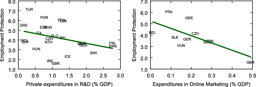
In Figure 1, I plot some suggestive evidence on this negative relationship between firing costs and innovation. In particular, I plot the relationship between the strictness of employment protection legislation taken from the OECD, and two measures that fit well the broad definition of innovation used in my paper: R&D expenditures (left panel) and firms’ spending on online marketing (right panel). In both cases, countries with high levels of firing costs show lower spending on innovation.Footnote 4 This is what happens in the model. In the baseline economy, with firing costs equal to the calibrated value of 2.5 monthly wages, investment in innovation is 2.7% lower than in the frictionless economy, making the average firm-level productivity to drop by 1.4%. When firing costs are of 1 year’s wage, innovation expenses and average productivity fall by 8% and 4.5%, respectively.
Firing costs and firms’ investments in growth-generating activities. Source: (i) Employment Protection refers to the sum of the OECD strictness of employment protection legislation indicators for permanent and temporary contracts; (ii) Private expenditures in R&D is taken from the OECD Main Science and Technology Indicators Database; (iii) Expenditures in Online Marketing is taken from Greece (Reference Grece2016).

To quantify how much of the estimated aggregate effects of firing costs is accounted for by endogenous changes in the dynamics of firms’ productivity, I simulate an economy with positive firing costs but fixing the innovation choices from the frictionless economy. This makes the law of motion of productivity to be unaffected by changes in the firing cost. In this new economy, the fall in aggregate productivity is of 2.4%, substantially lower than in a model with endogenous innovation where firms can adjust their innovation choices. This means that 36% of the drop in aggregate productivity is explained by changes in the dynamics of productivity.
However, the economy with exogenous innovation is still not comparable to a standard firm dynamics model with the typical AR(1) process for productivity. The reason is that in the economy with exogenous innovation, the law of motion of productivity is not affected by firing costs but differs across firms, as it is taken from the endogenous choices of firms in the frictionless economy. To quantitatively asses the contribution of these nonlinearities in accounting for the overall fall in aggregate productivity, I repeat the main experiment of the paper imposing an AR(1) process for firm productivity.Footnote 5 Thus, the only difference between this new economy and the economy with exogenous innovation is that in the latter the law of motion of productivity is different for different firms. Making the dynamics constant across firms reduces substantially the impact of firing costs. In particular, a firing cost of 2.5 monthly wages generates a fall in aggregate productivity of 1.64% relative to the frictionless economy, raising to 5.5% when firing costs are of 1 year’s wage. These effects represent between 45% and 50% of the aggregate productivity fall in the baseline economy.
In sum, this article uses a firm dynamics model with endogenous productivity dynamics to quantify the aggregate impact of firing costs. In the model, firms are able to affect the distribution of next period’s productivity, which implies that the law of motion of productivity is different across firms and can potentially be affected by firing costs. Both features contribute significantly to the aggregate effects of firing costs. These findings suggest that models with exogenous productivity processes may largely underestimate the effects of frictions/policies such as firing cost.
2. Literature review
There is a large literature that evaluates the role of different policies and frictions in accounting for aggregate productivity differences across countries [Guner et al. (Reference Guner, Ventura and Xu2008), Restuccia and Rogerson (Reference Restuccia and Rogerson2008), Hsieh and Klenow (Reference Hsieh and Klenow2009), Bartelsman et al. (Reference Bartelsman, Haltiwanger and Scarpetta2013), Hsieh and Klenow (Reference Hsieh and Klenow2014) and García-Santana et al. (Reference García-Santana, Moral-Benito, Pijoan-Mas and Ramos2016)]. While many of these papers measure policy distortions through “wedges”, some others specify particular policies.Footnote 6 One of the policies that has attracted more attention is employment protection, starting with the analysis of firing costs of Hopenhayn and Rogerson (Reference Hopenhayn and Rogerson1993). The distortion introduced by firing taxes on firms’ hiring and firing decisions is well established in the literature, both empirically [Haltiwanger et al. (Reference Haltiwanger, Scarpetta and Schweiger2014)] and theoretically [Bentolila and Bertola (Reference Bentolila and Bertola1990)]. These distortions prevent firms from operating at their optimal scale, worsening the allocation of labor across firms, and damaging aggregate productivity.
The literature studying the impact of firing costs on aggregate productivity typically finds moderate effects [Hopenhayn (Reference Hopenhayn2014)]. However, aggregate productivity losses may be larger when the productivity distribution of firms is endogenous, and thus, potentially affected by the policy. The reason is that firing costs may not only distort the allocation of workers but also the incentives of firms to invest in risky growth-generating activities—such as innovation, marketing campaigns, launching new products, etc.—changing the distribution of productivity itself. This additional channel, which is the focus of this paper, was first explored by Da-Rocha et al. (Reference Da-Rocha, Diego and Marina2019), who study the aggregate implications of firing costs in a model with size-dependent productivity dynamics. My paper differs from theirs in two margins. First, I consider a model with a continuum of potential firm size, while they consider a model where firms can either be small or large. Second, in their paper, the law of motion of firms’ productivity is size-dependent, but the difference between large and small firms is exogenous. In my paper, large and small firms will have different laws of motion for their productivities endogenously, as a result of different innovation choices which are affected by the introduction of firing costs.
More generally, my paper relates to a recent literature that explores how frictions affect aggregate productivity not only through the efficiency in the allocation of resources, but also through a direct effect on the distribution of firm-level productivity itself. For instance, López-García et al. (Reference López-García, Puente and Gómez2007) and Mukoyama and Osotimehin (Reference Mukoyama and Osotimehin2019) endogenizes the way in which frictions affect firm’s productivity dynamics by including an innovation technology similar to the one in Grossman and Helpman (Reference Grossman and Helpman1991), Aghion and Howitt (Reference Aghion and Howitt1992) and Atkeson and Burstein (Reference Atkeson and Burstein2010). Ranasinghe (Reference Ranasinghe2014) extends the Hopenhayn and Rogerson (Reference Hopenhayn and Rogerson1993) framework by allowing firms to invest in innovation, which changes the parameters of a flexible parametric distribution driving the next period’s distribution. Gabler and Poschke (Reference Gabler and Poschke2013) study the effects of firing costs, among other frictions, using a firm dynamics model in which firms can engage in experimentation and discard negative productivity shocks.
My paper contributes to this literature by making the distribution of firm-level productivity entirely driven by firm choices, including the degree of uncertainty faced by firms. This has two main implications. On the one hand, it allows my model to generate a sufficiently large downward risk while keeping the firms’ size distribution realistic. This is particularly relevant for the analysis of firing costs since this friction introduces asymmetric adjustment costs. On the other hand, the parameters governing the innovation process have a clear interpretation and can be identified using moments on firm size and hiring and firing choices. The innovation process used in this paper is also computationally convenient as it generates closed-form solutions for innovation choices. Thus, the model can be used to study the effects of different policies and friction accounting for their effects on the productivity distribution of firms without adding model complexity.
Finally, my paper is related to the game theory literature from which I borrow the “control cost” approach used to model productivity dynamics. This modeling device is used to model equilibria in which agents optimally make errors under the assumption that precision in decision-making is costly. In this approach, choices are conceived as a random variable over a feasible set of alternatives—which in my setting are the different levels of productivity—, and the cost is given by the precision of this random variable. In Costain et al. Reference Costain, Nakov and Petit(2022), we implement this idea to model price and wage adjustment decisions in an otherwise standard new-keynesian framework with heterogeneous agents. Turen (Reference Turen2019) models costly information acquisition in a price-setting problem using a “control cost” framework. To the best of my knowledge, my paper is the first that uses this approach to model the dynamics of firm-level productivity.
3. The model
This section presents an extension of the workhorse general equilibrium model of Hopenhayn and Rogerson (Reference Hopenhayn and Rogerson1993) in which I introduce an innovation technology that allows firms to invest in both the probability and the outcome of innovation.
3.1 Overview
The economy is populated by a continuum of firms of unit mass, characterized by a profitability factor, denoted by
 $d$
, and a number of workers hired in the past,
 $n$
. The term
 $d\in \mathbb{D}\equiv \{d_1,d_2,\dots,d_D\}$
is a factor that increases revenues for given inputs, so it captures both productivity (i.e. technology) and demand factors (i.e. taste). For simplicity in the exposition, I will refer to
 $d$
as firm’s productivity throughout the rest of the paper.
Given an initial state
 $(d,n)$
, firms decide on hirings/firings, produce, and collect profits. Then, they are hit by an exit shock. With probability
 $1-\delta \in (0,1)$
, the firm continues in the market and makes innovation decisions. With probability
 $\delta$
, the firm exists and it is immediately replaced by a new firm. Entrants start with no workers and an initial productivity drawn from
 $\log (d_0)\sim \eta ^0$
with
 $E[d_0] = \mu _0$
.
3.2 Firms
Firms produce a homogeneous good, and its price is normalized to 1. This good is used both to consume and to invest in innovation. It is produced using a decreasing returns to scale technology,
 $y(d,n) = d^{1-\gamma }n^{\gamma }$
, where
 $\gamma \in (0,1)$
the degree of returns to scale. Firms’ operating profits are given by
 \begin{equation} \Pi (d,n,n') \ = \ y(d,n') \ - \ w n' \ - \ \kappa _Fw\max \{0,n-n'\}, \end{equation}
where
 $n'$
is the number of workers involved in production in this period,
 $w$
is the wage rate, and
 $\kappa _Fw$
is the per-worker firing cost. Using this profit function, the value of a firm with productivity
 $d$
and
 $n$
workers is given by
 \begin{equation} V(d,n) \ = \ \max _{n^{\prime}} \ \ \Pi (d,n,n') \ + \ \beta (1-\delta )\mathcal{I}(d,n')\ + \ \beta \delta V_E(n'), \end{equation}
where
 $\beta \in (0,1)$
is the subjective discount factor,
 $\mathcal{I}(d,n)$
is the value of a firm with state
 $(d,n)$
before the innovation stage, and
 $V_E(n)=-w\kappa _F n$
captures the value of exit for a firm with
 $n$
workers.Footnote 7
3.3 Productivity dynamics
After production and the realization of the exit shock, firms enter the innovation stage. At this stage, firms decide how much resources to spend in improving their productivity prospects. If a firm decides to invest no resources in innovation, productivity would evolve according to an exogenous distribution
 $\eta$
that satisfies
 \begin{equation*} \mathbb {E}(d'|d) \ = \ \sum _{i = 1}^D \eta (d'|d)d_i \ = \ d(1-\mu ). \end{equation*}
where
 $\mu \gt 0$
is the depreciation rate of productivity. This assumption has an important implication: firms that decide to spend no resources in innovation expect their productivity to fall. In other words, productivity growth in this model only arises as a result of innovation, since the reverse-to-the-mean effect of the standard AR(1) productivity process used in the literature is not present.
Innovation consists of choosing both the probability and the outcome of innovation, defined as a distribution over next period’s productivity. I denote the probability of innovation as
 $\lambda \in [\bar{\lambda },1]$
, where
 $\bar{\lambda }\in (0,1)$
is a default innovation probability. The outcome of innovation is the distribution
 $\pi =(\pi _1,\pi _2,\dots,\pi _D)$
, satisfying:
 \begin{equation} \sum _{i=1}^D \pi _i=1. \end{equation}
where
 $\pi _i$
is the probability of drawing a productivity level of
 $d_i$
next period. Therefore, the productivity’s law of motion for firm that innovates is a combination of
 $\pi$
and
 $\eta$
. In particular, the firm draws the next period’s productivity from the distribution
 $\pi$
with probability
 $\lambda$
, and from
 $\eta$
with probability
 $1-\lambda$
. The choice of
 $\lambda$
can be thought as the extensive margin of innovation, and the choice of
 $\pi$
as the intensive one. Another valid interpretation would be to think of
 $\lambda$
as the probability of generating a new idea, and
 $\pi$
as the implementation of such idea.
Innovation problem
Let
 $\mathcal{I}^{I}(d,n)$
be the value of firm that innovates and
 $\mathcal{I}^{N}(d,n)$
be the value of not innovating. The innovation problem reads as
 \begin{eqnarray} \mathcal{I}(d,n) & = & \max _{ \lambda } \ \ \lambda \ \underset{}{\underbrace{\underset{}{\left ( \max _{\{\pi _i\}_{i=1}^D} \ \sum _{i=1}^D\pi _i V(d_i,n) - \mathcal{D}(\pi ||\eta ) \right ) }}_{\text{{$\mathcal{I}^{I}(d,n)$}}}}\ + \nonumber \\ && \hspace{4cm}\ + \ (1-\lambda )\underset{}{\underbrace{\underset{}{\left ( \sum _{i=1}^D \eta (d_i|d) V(d_i,n) \right )}}_{\text{{$\mathcal{I}^N(d,n)$}}}} - \mathcal{D}(\lambda ||\bar{\lambda }), \end{eqnarray}
subject to
 $\lambda \in [\bar{\lambda },1]$
and equation (3). The result of this maximization problem is a probability of innovation
 $\lambda (d,n)$
and a distribution of next period’s productivity
 $\pi (d'|d,n)=(\pi _1,\pi _2,\dots,\pi _D)$
, where
 $\pi _i=\pi (d_i|d,n)$
.
Innovation cost
The cost of choosing
 $\lambda$
is given by
 $\mathcal{D}(\lambda ||\bar{\lambda })$
, defined as proportional to the Kullback–Leibler divergence measure, or relative entropy, between
 $\lambda$
and
 $\bar{\lambda }$
:
 \begin{equation} \mathcal{D}(\lambda ||\bar{\lambda }) \ = \ \underset{}{\kappa _I \left [\lambda \log \left ( \frac{\lambda }{\bar{\lambda }}\right ) + (1-\lambda ) \log \left ( \frac{1-\lambda }{1-\bar{\lambda }}\right )\right ]},\\ \end{equation}
where
 $\kappa _I$
is the innovation cost, given by
 $\log \kappa _I=\log \kappa _0 + \kappa _1 \log d$
, with
 $\kappa _0\gt 0$
and
 $\kappa _1\gt 0$
. Assuming
 $\kappa _1\gt 0$
implies that cost of innovation is higher for high productivity firms, which is consistent with the lower growth rate of larger firms.Footnote 8 The intuition behind this assumption is that high productivity firms find it more difficult to generate ideas that could improve their already high level of productivity.
Similarly, the cost of choosing the distribution
 $\pi (d'|d,n)$
is given by
 $\mathcal{D}(\pi ||\eta )$
:
 \begin{equation} \mathcal{D}(\pi ||\eta ) \ = \ \kappa _I\left [\sum _{i=1}^D \pi _i \log \left (\frac{\pi _i}{\eta _i}\right )\right ], \end{equation}
Note that the innovation cost,
 $\kappa _I$
, is the same for both the extensive and the intensive margin. The main implication of this assumption is that the timing of choices does not affect the results [Costain (Reference Costain2017)].Footnote 9 Moreover, assuming equal costs implies that any combination of
 $\pi$
and
 $\lambda$
can be expressed as a single distribution.Footnote 10
Note also that equation (6) implies that setting a probability
 $\pi _i\lt \eta _i$
would reduce the cost
 $\mathcal{D}(\pi ||\eta )$
. However, recall that
 $\pi$
is a proper probability distribution. Thus, setting a low
 $\pi _i$
would require setting a larger value somewhere else in the distribution, increasing the total cost. In fact, it can be shown that
 $\mathcal{D}(\pi ||\eta )\gt 0$
for any distribution
 $\pi$
different from
 $\eta$
, and 0 if (and only if)
 $\pi \equiv \eta$
. The same reasoning applies to the choice of
 $\lambda$
in equation (5), where
 $\mathcal{D}(\lambda ||\bar{\lambda })=0$
if (and only if)
 $\lambda = \bar{\lambda }$
.Footnote 11
In sum, I make two assumptions regarding innovation cost. First, I define the cost of innovation to be increasing in firm’s productivity, which allows the model to generate lower growth rates among large firms as explained before. Second, I assume that this cost is proportional to the Kullback–Leibler divergence measure. This measure has become very popular in models of state-dependent pricing literature or rational inattention [Turen (Reference Turen2019) and Costain et al. (Reference Costain, Nakov and Petit2022)]. The reason for this popularity is that the Kullback–Leibler divergence measure allows for closed-form solutions for equilibrium objects that would, otherwise, require a high computational cost. This advantage is also applicable to my model where, as in some models of state-dependent pricing or rational inattention, one of the policy functions is a distribution.
To solve the innovation problem, I first solve the choice of the next period’s productivity distribution for innovating firms. Then, given the choice of
 $\pi$
, and thus, the value of innovating, I solve the choice of the innovation probability.
Choice of next period’s productivity distribution,
 $\pi$

The choice of the next period’s distribution for innovative firms consists of choosing each probabilities
 $\pi _i$
in the distribution
 $\pi =(\pi _1,\pi _2,\dots,\pi _D)$
. The first order condition of (4) with respect to the probability
 $\pi _i=\pi (d_i|d,n)$
is
 \begin{equation} V(d_i,n) \ = \ \kappa _I \left [ 1 + \log \left (\frac{\pi (d_i|d,n)}{\eta (d_i|d)}\right ) \right ] + \xi, \end{equation}
where
 $\xi$
is the multiplier on the constraint (3). The left-hand side of equation (7) is the marginal gain from increasing
 $\pi (d_i|d,n)$
, which equals the value of a firm with productivity
 $d_i$
. The right-hand side is the marginal cost, which is the sum of two terms: the “direct” innovation cost associated with the choice of
 $\pi (d_i|d,n)$
and the cost associated with the constraint, captured by
 $\xi$
. Using the first-order conditions for
 $(\pi _1,\pi _2,\dots,\pi _D)$
described by equation (7) in the constraint (3), and after some rearrangement, one finds
 \begin{equation} \pi (d_i|d,n) \ = \ \frac{\eta (d_i|d)\exp \left (V(d_i,\underset{}{n})/\kappa _I\right ) }{\sum _{j=1}^D \eta (d_j|d)\exp \left ( V(d_j,\underset{}{n})/\kappa _I \right ) }. \end{equation}
The chosen distribution is a transformation of the default distribution
 $\eta$
. In particular, firms will choose to increase the probability of those
 $d_i$
that imply larger continuation values, and decrease those that deliver lower
 $V(d_i,n)$
. Yet, this transformation is not linear—that is, the chosen distribution is not just a shifted version of
 $\eta$
. The reason is that firms want to increase the probability of a high
 $d_i$
more than what they can decrease it for a low
 $d_i$
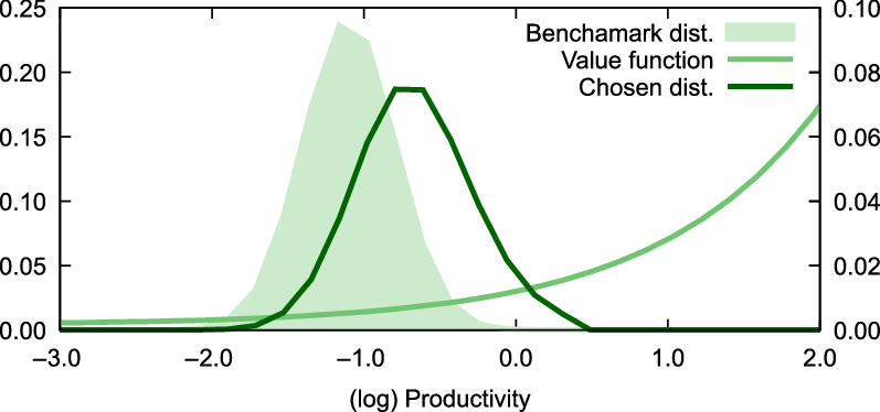
. This can be clearly seen in Figure 2. Taking an arbitrary firm, Figure 2 presents the benchmark distribution
 $\eta$
(shaded area), the continuation value of the firm
 $V(d_i,n)$
(light line) and the chosen distribution
 $\pi$
(dark line). The chosen distribution
 $\eta$
is shifted to the right relative to
 $\eta$
, but it is also more dispersed.
Choice of next period’s productivity distribution,
 $\pi$
. Notes: The shaded area represents the benchmark distribution
 $\eta$
faced by a firm with productivity
 $d=-1$
and 5 employees, the dark line the chosen distribution,
 $\pi$
, and the light line plots the (normalized) value function for the different values of productivity. For this exercise, I used the baseline calibration, presented in Section 4.

To understand why the chosen distribution is more dispersed, one needs to look at the tails of both distributions. Firms want to increase the probability of larger values of
 $d'$
, but to do so, firms have to reduce the probability somewhere else in the distribution. However, the probability in the left tail of the benchmark distribution cannot be reduced sufficiently to accommodate the desired increase in the right tail, as the cost of setting
 $\pi (d_i|d,n)=0$
if
 $\eta (d_i|d)\gt 0$
would be infinitely costly.Footnote 12 As a result, the chosen distribution has the same support as
 $\eta$
but a fatter right tail, yielding a more dispersed distribution.
Finally, using equations (8) and (6), we can write
 $\mathcal{I}^I(d,n)$
as
 \begin{equation} \mathcal{I}^I(d,n) \ = \ \kappa _{I}\log \left [ \sum _{i = 1}^D \eta (d_i|d)\exp \left ( V(d_i,\underset{}{n})/\kappa _I\right ) \right ] \end{equation}
Note that Jensen’s inequality implies that
 $E\left [\exp (x)\right ] \gt \exp \left [E(x)\right ]$
for any non-degenerate random variable, and therefore,
 $\mathcal{I}^I(d,n) \gt \sum _{i=1}^D \eta (d_i|d) V(d_i,\underset{}{n}) = \mathcal{I}^N(d,n)$
, so that firms will always prefer to innovate.Footnote 13
Choice of the innovation probability,
$\lambda$

The choice of the innovation probability consists of setting the probability
 $\lambda$
with which the firm can choose the next period’s productivity distribution. The first-order condition of equation (4) with respect to the probability of innovation
 $\lambda$
is
 \begin{equation*} \mathcal {I}^{I}(d,\underset {}{n}) -\mathcal {I}^{N}(d,\underset {}{n}) = \kappa _I \left [ \log \lambda (d,n) - \log \bar {\lambda } - \log (1-\lambda (d,n)) + \log (1-\bar {\lambda })\right ], \end{equation*}
where the left-hand side are the gains from innovation, equal to the marginal product of
 $\lambda (d,n)$
, and the right-hand side is the marginal cost. Rearranging terms:
 \begin{equation} \lambda (d,n) \ = \ \frac{\bar{\lambda }\exp \left (\mathcal{I}^{I}(d,\underset{}{n})/\kappa _I\right ) }{\bar{\lambda }\exp \left (\mathcal{I}^{I}(d,\underset{}{n})/\kappa _I\right ) + (1-\bar{\lambda })\exp \left (\mathcal{I}^{N}(d,\underset{}{n})/\kappa _I \right ) }. \end{equation}
The probability of innovation
 $\lambda (d,n)$
is increasing in the difference between the value of innovating,
 $\mathcal{I}^{I}$
, and the value of not innovating,
 $\mathcal{I}^{N}$
. Moreover, equation (10) implies that
 $\lambda (d,n)\gt \bar{\lambda }$
for any
 $(d,n)$
, since
 $\mathcal{I}^I(d,n) \gt \mathcal{I}^N(d,n)$
.
3.4 Households
The household problem closely follows Hopenhayn and Rogerson (Reference Hopenhayn and Rogerson1993) and Da-Rocha et al. (Reference Da-Rocha, Diego and Marina2019). There is a household with a continuum of members who own the firms, consume, and supply labor. The problem of the household is
 \begin{eqnarray*} U & = & \underset{}{\max _{C,L} \ \ \ln C \ - \ \theta L} \nonumber \\ && \text{s.t.} \ \ \ \ C \ = \ wL + F + \Pi, \end{eqnarray*}
where
 $C$
is household consumption,
 $L$
is the total labor supply,
 $F$
are the total firing taxes, and
 $\Pi$
are firms’ profits. The parameter
 $\theta \gt 0$
captures the disutility of labor supply. The optimal labor choice is characterized by
 $w=\theta C$
.
3.5 Stationary equilibrium
Let
 $x=(d,n)$
be the state vector,
 $\mathcal{X}\equiv \mathbb{D}\times \mathbb{R}_{\geq 0}$
be the state space, and
 $F$
be the distribution of firms over
 $\mathcal{X}$
. For simplicity in the exposition, I consider a discretized state space so that
 $F(x)$
is the mass of firms with state
 $x$
. The law of motion of the distribution of firms is
 \begin{equation*} F^{\prime }(x) \ = \ (1-\delta )\sum _{z\in \mathcal {X}} \Gamma (x|z)F(z) \ + \ \delta \Gamma ^E(x), \end{equation*}
where
 $F'$
is the next period’s distribution of firms,
 $\Gamma (x|z)$
is the incumbents’ transition probability between states
 $z$
and
 $x$
, derived from firm choices, and
 $\Gamma ^E$
is the distribution of entrants that results from the discretization of the distribution of
 $d_0$
.
The equilibrium of this economy is given by a wage rate, a distribution of firms over the state space, and a set of firm’s policy functions (for
 $n'$
,
 $\lambda$
and
 $\pi$
) such that (i) policy functions solve firms’ problem, (ii) the household first order condition is satisfied, (iii) labor market clears, and (iv) the distribution of firms over the state space
 $\mathcal{X}$
is invariant,
 $F'(x) = F(x)$
,
 $\forall x\in \mathcal{X}$
.
4. Calibration
The model is calibrated to the Spanish economy, using data from the Central de Balances dataset. This is a panel of nonfinancial Spanish firms, prepared by the Bank of Spain, including balance sheet information, income statement, and some firm characteristics (sector, age, etc). The panel covers the years 1995 to 2015 and provides an excellent representation of the Spanish productive sector.Footnote 14 Since Spanish employment is highly volatile, I restrict the sample to the years between 2005 and 2007 in order to avoid the Spanish boom (2000–2005) and the financial crisis. The model period is set to 1 year.
4.1 Exogenous parameters
I set the discount factor to
 $\beta =0.95$
.Footnote 15 I set the degree of returns to scale to
 $\gamma =0.6$
, somewhat lower than in Hopenhayn and Rogerson (Reference Hopenhayn and Rogerson1993), but within the standard values in the literature.Footnote 16 I normalize the equilibrium wage rate to 1 and make
 $\theta$
be such that the household first-order condition is satisfied in the benchmark equilibrium. Finally, I set the exit probability parameter to 7.56% so that the average firm age in the model is 9.7 years, as in the data.
4.2 Endogenous parameters
The remaining parameters are internally calibrated using the model. I calibrate the parameters of the initial distribution of productivity, the firing cost parameter, the benchmark probability of innovation, the innovation cost parameters, and the benchmark distribution,
 $\eta$
. The latter is modeled as a discretized unit root process:
 \begin{equation} \log (d') \ = \ \log (d) - \mu + \sigma \epsilon. \end{equation}
The initial productivity distribution is defined as a discretized normal distribution with parameters
 $\mu _0$
and
 $\sigma _0^2$
, such that
 $\log (d_0)\sim N\left (\log (\mu _0)-\frac{1}{2} \sigma _0^2,\sigma _0^2 \right )$
.
The parameter vector,
 $\Omega = (\mu _0,\sigma ^2_0,\kappa _F, \bar{\lambda },\kappa _0,\kappa _1, \mu, \sigma ^2)$
, is chosen such that the sum of squared differences between a set of model-generated moments and their empirical counterparts is minimized:
 \begin{equation*} \min _{\Omega } \ \sum _{i=1}^{M} \left (\frac {m_i(\Omega )-\bar {m}_i}{\bar {m}_i }\right )^2, \end{equation*}
where
 $M$
is the number of moments, and
 $m_i(\Omega )$
and
 $\bar{m}_i$
are the model-generated and empirical
 $i$
-th moments, respectively.
Moment selection and identification
The main limitation of my data is that it lacks information on firms’ innovation choices. Furthermore, given the broad meaning of innovation in this paper, it is not clear what type of information one should use. However, the model establishes a clear link between productivity and size, allowing me to discipline the innovation technology using employment data, as in Garcia-Macia et al. (Reference Garcia-Macia, Hsieh and Klenow2019). Note that hiring and firing choices in my model only depend on productivity, so targeting the dynamics of employment would pin down the dynamics of productivity. For instance, given that productivity growth only emerges from innovation, the share of hiring firms and their growth rate are very informative about the share and growth rate of innovators. Thus, the model is calibrated to match the share of hiring firms and the hiring rate, defined as the ratio between newly hired workers and previous employment.
Innovation cost is assumed to be increasing in firm productivity. To control for the strength of this effect, I target the size distribution of firms. Note that, if innovation is equally costly for high- and low-productivity firms, high-productivity firms would grow faster than low-productivity ones, generating a bimodal firm size distribution. Given the focus of this paper on firing cost, firing behavior is particularly relevant for the analysis. I match the share of firing firms and the firing rate, defined analogously to the hiring rate. Finally, given that innovation is particularly flexible, it is important to control for the shape of the resulting distribution of next period’s productivity. To do so, I match the average and the coefficient of variation of firm size, both for the whole population of firms and for entrants.
Although all moments are affected by all the parameters, some relationship between specific parameters and moments can be postulated.Footnote 17 The average productivity of entrants,
 $\mu _0$
, is particularly relevant to match the average size of entrants. The variance of the initial productivity draw,
 $\sigma ^2_0$
, drives the dispersion in firm size among entrants, so it is key to match the coefficient of variation of firm size among entrants. The variance of the benchmark distribution,
 $\sigma ^2$
, controls the dispersion of the chosen distribution among innovators, and thus, drives the overall dispersion in firm size. The parameter
 $\kappa _0$
limits how much innovative firms can grow and, as argued before, is informative to match the hiring rate observed in the data. The parameter
 $\kappa _1$
controls the rate at which the cost of innovation increases with firm’s productivity, and thus, the ability to grow among high-productivity firms, driving the firm size distribution. Since productivity growth only emerges from innovation, the share of innovators is very informative about the share of hiring firms. The default probability of innovation,
 $\bar{\lambda }$
, is key for the overall probability of innovation in the model and thus, it is very informative about the share of hiring firms. Among those firms that do not innovate, the productivity depreciation parameter,
 $\mu$
, drives the size in the productivity fall, and therefore, it is very informative about the firing rate, which is key to control the magnitude of downwards risk. Finally, the firing cost parameter,
 $\kappa _F$
, drives the share of firms firing workers.
Parameter values and model fit
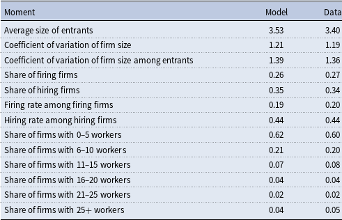
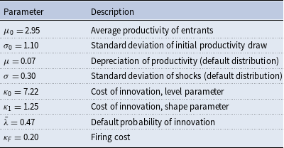
Table 1 presents the model fit and Table 2 collects the estimated parameters. The model closely matches the moments concerning firing and hiring behavior, and the size distribution of firms is also closely matched.Footnote 18 This is particularly relevant since it provides support for the innovation technology used in the paper. Furthermore, the model generates a distribution of firm size that matches not just the average firm size, but also the dispersion in employment, which provides further support to the innovation technology. In the next section, I discuss the main predictions generated by my innovation technology and show that these predictions are consistent with the existing empirical evidence on firm growth.
Calibration. Model fit

Calibration. Parameter values

The firing cost parameter is calibrated to 0.20. This means that the cost of firing one worker equals 2.5 monthly wages. According to Spanish labor regulations, a dismissed worker has the right to receive 40 days of wages per year working in the firm. Note, however, that the Spanish economy is characterized by the heavy use of temporary workers, whose firing costs are either zero or very small. Thus,
 $\kappa _F$
should be interpreted as an average firing cost for both temporary and permanent workers. The depreciation rate of productivity,
 $\mu$
, is calibrated to 0.07, meaning that those firms that do not invest in innovation expects to loss 7% of its current productivity next period. The standard deviation of productivity under the default distribution is 0.3, similar to Poschke (Reference Poschke2009) who also assumes a unit root process for firm’s productivity.
The magnitude of
 $\kappa _0$
and
 $\kappa _1$
do not have a clear interpretation. Nevertheless, they imply that firms in the baseline economy spend 16% of total output in innovation.Footnote 19 Although this may be too high for innovation expenses, it should be noticed that innovation in this model includes all sorts of firm actions aimed at increasing profitability prospects, and not only product or process innovation as typically assumed in innovation papers. For instance, Mukoyama and Osotimehin (Reference Mukoyama and Osotimehin2019), who also consider a broad concept of innovation similar to mine, find an innovation-to-output ratio of 12%.
The default probability of innovation is 0.47, which is 9 p.p. lower than the average innovation probability in the baseline economy. Given the structure of the innovation problem, most innovation investments are devoted to the choice of the next period’s productivity. This is because the cost of choosing a distribution
 $\pi$
is incorporated in the value of innovating lowering gains for innovation, as shown in equation (4).
5. Results
Before analyzing the effects of firing cost, it is worth describing firms’ innovation behavior in the baseline equilibrium to illustrate how my approach to model firm innovation can generate realistic productivity dynamics.Footnote 20
5.1 Endogenous productivity dynamics
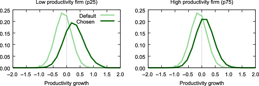
Many papers in the literature of firm growth document the negative (unconditional) relationships between firm size and growth and between firm size and volatility of growth.Footnote 21 The model is consistent with these facts. Figure 3 presents the default and chosen distributions of productivity growth for a low- and high-productivity firm (in the 25th and 75th percentile of the productivity distribution, respectively). The average productivity growth for those firms that innovate (thus, taking the chosen distribution
 $\pi$
) is as high as 0.22 for low productivity firms and 0 for high productivity firms, who just offset the negative productivity trend on average. At the same time, the standard deviation of productivity growth is 0.45 for low productivity firms and 0.35 for high productivity ones. This result is driven by the fact that the cost of innovation is assumed to be increasing in firm’s productivity.
Productivity growth. Next period’s productivity distribution. Notes: The
 $x$
-axis refers to the difference in log productivity
 $\Delta \log d$
. The dark line is the chosen next period’s distribution
 $\pi$
for a low and a high productivity firm. The light line represents the default distribution,
 $\eta$
, given by equation (11), which is the same for low and high-productivity firms by assumption.

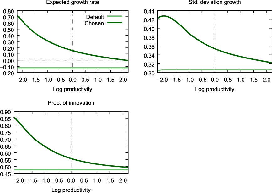
This can be seen more generally in Figure 4, where I plot the expected productivity growth rate, the standard deviation of firm productivity growth, and the probability of innovation by firm productivity in the baseline economy in which
 $\kappa _F=0.20$
. Later we will discuss how these figures change when we increase/decrease the firing cost. Three main predictions arise from the model: (i) low productivity firms innovate more frequently, (ii) they undertake more aggressive innovations, and (iii) their innovations are riskier, as measured by the expected productivity growth and the standard deviation of expected firm productivity growth, respectively. As a result, low-productivity (small) firms in the model grow faster and face higher uncertainty. This does not mean that small firms spend more on innovation. For instance, a firm with 10 workers spends 40% less in innovation than a firm with 30 workers.Footnote 22 This is because high-productivity firms prefer to lower the risk they face, which is also costly.
Innovation choices by firm productivity. Notes: I compute the expected productivity growth rate and standard deviation of productivity growth for each point in the discretized state space using the corresponding distribution of next period’s productivity,
 $\pi$
(chosen) or
 $\eta$
(default), and then average across firm size for each value of
 $d$
. The probability of innovation is also averaged across size for every value of
 $d$
, where the default probability is
 $\bar{\lambda }$
and the chosen one is given by
 $\lambda (d,n)$
. Figure B.5 replicates these graphs by number of employees.

Figure 4 highlights the importance of allowing firms to have (partial) control over the whole distribution of next period’s productivity. Models based on Atkeson and Burstein (Reference Atkeson and Burstein2010) allow firms to affect the probability of innovation while keeping the “size” of the innovation fixed. Alternatively, once could fix the probability of innovation and allow firms to invest in the average productivity growth. However, the volatility of productivity growth is constant across firms and unaffected by the distortion in both cases. In this model, firms endogenously face different degrees of uncertainty, which is key to account for the effects of firing costs (Bentolila and Bertola, Reference Bentolila and Bertola1990).
5.2 Aggregate effects of firing costs
The main goal of this article is to better understand the aggregate consequences of firing costs. To facilitate the exposition and the comparison with previous literature, I simulate the frictionless economy, in which
 $\kappa _F=0$
, and compare it with an economy with positive firing costs. In this exercise, the main object of interest is aggregate productivity. Following Da-Rocha et al. (Reference Da-Rocha, Diego and Marina2019), I define aggregate productivity as
 \begin{equation} \text{aggregate productivity} \ = \ \left (\int _{x\in \mathcal{X}} d(x)^{1-\gamma } s(x) dF(x) \right )^{\frac{1}{1-\gamma }}, \end{equation}
where
 $x=(d,n)$
is the state vector of the firm, and
 $F(x)$
is the stationary mass of firms with state
 $x$
, satisfying
 $\int _xdF(x) = 1$
.Footnote 23
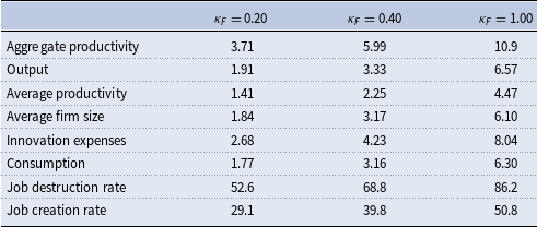
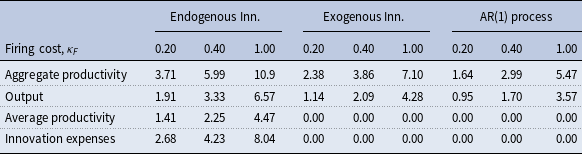
Table 3 collects the results of this experiment. Table entries represent the percentage (negative) change in the corresponding variable relative to the frictionless economy. In the first column, I compare the frictionless economy with the one that arises from the calibration exercise presented in Section 4, in which the firing cost parameter is
 $\kappa _F=0.20$
. The second column collects the results from simulating an economy in which I set the firing cost parameter to
 $\kappa _F=0.40$
, twice as large as the calibrated value. Finally, and to facilitate the comparison with the literature, I simulate an economy in which firing costs are equivalent to 1 year’s wage. All these results are general equilibrium outcomes.Footnote 24
Aggregate effects of firing cost (% fall relative to frictionless economy)

In line with the findings of previous literature, I find that firing costs damage aggregate productivity. In particular, the baseline level of firing costs, equivalent to 2.5 monthly wages, generates a 3.7% fall in aggregate productivity relative to the frictionless economy. Output and consumption also fall substantially, by almost 2%. These are large numbers compared to the literature. With a firing cost of 1 year’s wage, Da-Rocha et al. (Reference Da-Rocha, Diego and Marina2019) find a 4.2% fall in aggregate productivity and output, and Gabler and Poschke (Reference Gabler and Poschke2013) find fall in output and consumption of 2.5% and 4%, respectively. With that level of firing costs, I find a fall in aggregate productivity, output and consumption of 11%, 6.6%, and 6.3%, respectively. These comparisons, however, must be taken with caution. Both Da-Rocha et al. (Reference Da-Rocha, Diego and Marina2019) and Gabler and Poschke (Reference Gabler and Poschke2013) are calibrated to the USA, while I calibrate my model to Spanish data, and Da-Rocha et al. (Reference Da-Rocha, Diego and Marina2019) and I assume constant mass of firms and exogenous exit while Gabler and Poschke (Reference Gabler and Poschke2013) includes endogenous exit.
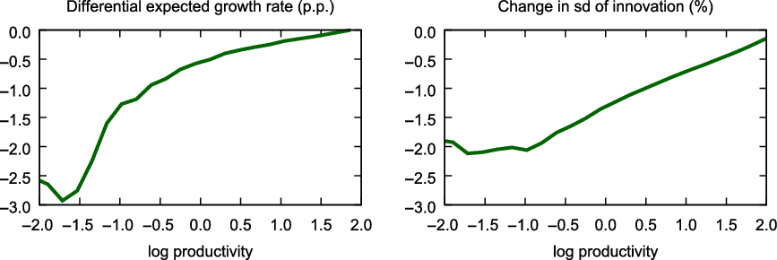
The main additional channel compared to previous papers is that firing costs in my model affect the whole productivity distribution by changing firms’ incentives to innovate.Footnote 25 In particular, firing costs make innovation riskier because the cost of a negative productivity shock increases. As a result, firms decide to decrease the dispersion in next period’s productivity at the expense of lowering potential productivity growth, generating a decrease in the (unweighted) average productivity of 1.4%. To see how firing costs shift firms’ innovation decisions, Figure 5 presents the differential expected productivity growth rate (left panel) and the differential standard deviation of next period’s productivity (right panel) between the frictionless economy and one in which firing costs are set to
 $\kappa _F=0.2$
.Footnote 26 The fall in expected productivity growth is of 3 p.p. for low productivity firms (and up to 10 p.p. if
 $\kappa _F=1$
) who lower the standard deviation of next period’s productivity distribution decreases by 2% (and 6% if
 $\kappa _F=1$
).Footnote 27
Innovation choices. Experiment,
 $\kappa _F=0.2$
vs.
 $\kappa _F=0$
. Notes: To compute the differences in expected productivity growth between non-innovative and innovative firms, I average expected growth over firm size for each productivity
 $d$
using the corresponding distribution of next period’s productivity (
 $\pi$
for innovative firms and
 $\eta$
for non-innovative firms) as in Figure 4. I do the same for computing the volatility of next period’s distribution.

Both the expected productivity growth and the volatility of next period’s productivity fall more among low productivity firms. This is because firing costs increase the cost of failure more intensively among low productivity firms, since these firms face a higher probability of having to fire workers—that is, the probability of drawing a level of productivity that induces firms to fire—in case of a negative productivity shock.Footnote 28 Because of this, low-productivity firms decide to focus their innovation on avoiding negative productivity shocks by reducing the risk of their innovation at the expense of productivity growth.Footnote 29 This effect of firing costs is substantially smaller for high-productivity firms, for whom firing workers is a very unlikely event. The differential response of high- and low-productivity firms highlights again the importance of allowing firms to control both the outcome and the risk of innovation.
Productivity and size are positively correlated, so the fall in expected productivity growth is also higher for small firms compared to large ones. When the firing cost parameter is set to
 $\kappa _F=0.2$
, the growth rate of productivity for firms with less than 10 workers falls by 0.93 p.p. relative to the undistorted economy, while that of firms with more than 10 employees decreases by 0.14 p.p. When the firing cost parameter is set to
 $\kappa _F=0.4$
, the growth rate of productivity falls by 1.1 p.p for firms with less than 10 workers and increases by 0.3 p.p. for firms with more than 10 workers, who benefit from lower wages.Footnote 30 These results show that small firms are particularly affected—consistent with larger effects among low productivity firms. The reason is that small firms face a higher probability of firing, and thus, face larger potential costs. Consequently, small firms endogenously choose to invest more on reducing the dispersion of next period’s productivity at the expense of lowering potential productivity growth.
The distorted economy also exhibits lower job destruction and creation rates (defined as total firings/hirings over total employment). In particular, the share of newly hired workers in the economy falls by 30%, from 18.3% to 12.6%, while the share of fired workers drops by more than 53%, from 10.7% to 5.1%. Since firms find it costlier to fire workers with
 $\kappa _F\gt 0$
, they decide to keep workers even if their size is larger than the optimal one. At the same time, firms below their optimal size decide not to hire due to precautionary motives. Since there is uncertainty about future productivity, firms know that they may need to fire in the future, which prevents them from hiring in the first place. Interestingly, the fall in job creation is less pronounced than that in job destruction, as in Bentolila and Bertola (Reference Bentolila and Bertola1990). These two distortions give rise to inefficiencies in the allocation of labor, which further damages aggregate productivity.
5.2.1 Sensitivity analysis
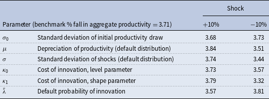
In this section, I check how robust the results presented in Table 3 are to changes in the calibrated parameter values.Footnote 31 In particular, I compare the aggregate productivity losses from firing costs of 2.5 monthly wages shocking each calibrated parameter at a time, first increasing it by 10%, and then lowering it by 10%. To ensure comparability, I recompute the disutility of labor supply,
 $\theta$
, so that the equilibrium wage is equal to 1 for each alternative calibration.
The results, collected in Table 4, suggest that effects of firing costs on aggregate productivity are very robust to changes in the calibrated parameters.Footnote 32 In general, changes in the parameter values that make innovation cheaper lower the overall impact of firing costs on aggregate productivity. This is the case for an increase in
 $\bar{\lambda }$
or a decrease in
 $\kappa _0$
,
 $\kappa _1$
,
 $\mu$
or
 $\sigma$
. The reason is obvious: for a given value of firing cost, a lower cost of innovation allows firms to grow more, making the fall in aggregate productivity smaller. For instance,
 $\kappa _1$
controls how costly it is to innovate for high-productivity firms. As it decreases, innovation becomes cheaper for those firms that are less affected by firing costs. Something similar happens when increasing the default probability of innovation: as
 $\bar{\lambda }$
increases, the cost of the extensive margin lowers, and firms use those resources to invest more in the intensive margin. In both cases, firms are able to reduce the probability of firing (by lowering the probability of a decrease in productivity), shrinking the overall effect of firing costs.
Sensitivity analysis (% fall in aggregate productivity relative to frictionless economy)

One important parameter in the model, that is not included in the previous table, is the degree of returns to scale,
 $\gamma$
. In order to check the robustness of the results to changes in the value of
 $\gamma$
, I set a
 $\gamma =0.66$
(a 10% increase relative to its baseline value), recalibrate the rest of the parameters, and then compute the losses in aggregate productivity associated with firing costs. I find that aggregate productivity falls by 4.7%, 7.6%, and 13.6% for a level of firing costs equivalent to 2.5 monthly wages (
 $\kappa _F=0.2$
), 5 monthly wages (
 $\kappa _F=0.40$
), and 1 year wages (
 $\kappa _F=1$
), respectively.Footnote 33 These numbers are larger than the results presented in the first row of Table 3, suggesting that my choice of
 $\gamma$
is conservative.
5.3 What is the role of endogenous productivity dynamics?
Firm choices are affected by firing costs, including those regarding innovation. This means that firing costs may have an impact on aggregate outcomes that goes beyond the distortion in firing/hiring choices. Most papers studying the effects of firing costs and other frictions typically abstract from this indirect effect. The most extended assumption is that firms’ productivity follows an AR(1) process, which is not only unaffected by frictions, but also implies identical dynamics across firms.
It is natural to ask whether abstracting from the endogenous determination of productivity dynamics yields very different results. This section presents two experiments that quantify the impact of the (endogenous) changes in the dynamics of productivity as a response to firing costs, and of the differences in productivity dynamics across firms.
5.3.1 Exogenous innovation
To quantify the aggregate impact of firing costs through their effects on the dynamics of productivity, I repeat the experiments shown in section 5.2, fixing the innovation behavior from the frictionless economy. In short, I simulate a distorted economy in which I impose a law of motion for firm productivity given by
 \begin{equation*} d' \sim \begin {cases} \ \pi (d'|d,n;\kappa _F=0) & \text {w.p. } \ \lambda (d,n|\kappa _F=0) \\ \ \eta (d'|d) & \text {w.p. } \ 1-\lambda (d,n|\kappa _F=0) \end {cases} \end{equation*}
where
 $\lambda (d,n|\kappa _F=0)$
and
 $\pi (d'|d,n;\kappa _F=0)$
are the resulting innovation probabilities and distributions from the frictionless economy in which firing costs are set to zero. To ensure the comparability of these two economies, I also keep the cost of innovation fixed, which is now added as a fixed cost to the value of the firm. Results are collected in Table 5.Footnote 34 The first three columns collect the results from the exercise in section 5.2, in which innovation is endogenous, and thus, reacts to changes in firing costs. Columns 4 to 6 collect the results from changing firing costs in an economy in which I fix the innovation behavior that arises from the frictionless economy.
Aggregate effects of firing cost. Counterfactual economies (% fall relative to frictionless economy)

In the model with exogenous innovation, a level of firing costs of
 $\kappa _F=0.2$
implies a fall in aggregate productivity of 2.3% which is significantly lower than in a model with endogenous productivity dynamics. This fall in aggregate productivity represents a 65% of the estimated fall when innovation choices can react to changes in firing costs. In other words, changes in firms’ innovation choices account for 35% of the aggregate productivity losses associated with firing costs. Endogenous firm productivity dynamics are also important in accounting for the changes in aggregate output. In particular, the fall in aggregate output with exogenous innovation is equal to 1.1%, 2.1%, and 4.3% when the firing cost parameter equals 0.2, 0.4, and 1, respectively. These effects account for a 35–40% of the overall fall in aggregate output.
Given that innovation choices are fixed, the (unweighted) average productivity does not change when firing costs are introduced. In the baseline experiment, firms react to firing costs by reducing the innovation risk at the expense of potential growth, damaging the average productivity in the economy. This indirect effect of firing costs is not present in the exogenous innovation scenario, lowering the overall effect of firing costs on aggregate productivity and output.
Interestingly, the aggregate effects of firing costs when innovation is fixed are still large compared to previous literature. The main reason for this is that the dynamics of productivity when innovation is exogenous are the ones obtained in the frictionless economy, and thus, nonlinear. This means that the persistence and volatility of productivity are not constant across firms, as in models based on AR(1) productivity processes.Footnote 35
5.3.2 AR(1) productivity dynamics
To quantify the implications of the nonlinearity of productivity dynamics, I repeat the experiment in an economy with a standard AR(1) process for firm’s productivity. To do so, I solve the baseline economy with zero firing costs, and compute the (average) transition matrix for firm’s productivity.Footnote 36 Then, I find the AR(1) parameters that minimize the distance between the transition matrix obtained from the baseline economy with no firing costs and the one arising from the Tauchen’s discretization of the estimated AR(1) process.Footnote 37 The results from this experiment are presented in columns 7–9 of Table 5.
Using the estimated AR(1) process, I find that a firing cost of 0.2 yearly wages generates an aggregate productivity fall of 1.64% relative to the frictionless economy.Footnote 38 When firing costs are set to 0.4 and 1 year’s wage, aggregate productivity falls by 2.99% and 5.47%, respectively. These effects are substantially lower than in the economy with exogenous innovation. This means that nonlinearities in the dynamics of productivity are quantitatively very relevant in accounting for the aggregate impact of firing costs.
Note that the only difference between the economy with exogenous innovation and the one with an AR(1) process is that the dynamics are linear in the latter. This means that the differences in the aggregate productivity fall between these two alternative economies can be attributed exclusively to the nonlinearities in the dynamics of productivity. Using this decomposition, I find that the nonlinearities in productivity dynamics explain 15–20% of the overall fall in aggregate productivity.
Overall, allowing for an endogenous determination of productivity dynamics accounts for 50–55% of the aggregate impact of firing on productivity: endogenous changes in the dynamics of productivity account for 35% of the overall effect, while 15–20% is explained by differences in the law of motion of productivity across firms.
6. Conclusions
This article presented a firm dynamics model with endogenous productivity growth to analyze the aggregate effects of firing cost. Making the dynamics of productivity endogenous allows the model to capture both the static effects of firing taxes—allocative efficiency—as well as the dynamic effects of such friction—changes in the distribution of firms’ productivity. As opposed to the existing literature, my model allows firms to control not only the probability of innovation but also the outcome. The model parameters are calibrated to match the firm size distribution and key features of the hiring and firing behavior of Spanish nonfinancial firms. I show that my flexible innovation technology is able to generate a distribution of firm size that is very close to that in the data, both in terms of size and in terms of dispersion.
I use the calibrated model to quantitatively assess the aggregate effects of firing cost. I show that firing costs equivalent to its calibrated value of 2.5 monthly wages generates a 3.7% drop in aggregate productivity relative to the frictionless economy. When firing costs are equivalent to 1 year’s wage, the fall in productivity is of 10%. I show that the introduction of firing costs makes firms to shift their innovation efforts towards decreasing the risk they face, at the expense of lowering the potential productivity growth. Moreover, low productivity firms—as well as small firms—are the ones most affected by the policy. The reason is that the probability of having to fire next period is larger for these firms, so that firing costs increase their cost of innovation failure relatively more.
My model differs from standard firm dynamics models in that productivity dynamics are endogenous. This has two important implications. First, innovation choices, and therefore, the distribution of firms’ productivity itself, can be distorted by firing costs. Second, as opposed to the standard AR(1) process typically used in the literature, the dynamics of productivity in my model are (endogenously) nonlinear and different across firms. I show that changes in innovation choices account for 35% of the aggregate productivity losses associated with firing costs, while nonlinearities in the dynamics of productivity explains another 15–20%. This result suggests that researchers should take the effects of frictions on the dynamics of productivity into account when evaluating their aggregate effects. This article applies this idea to firing cost, but it can be extended to any other frictions, such as distortionary corporate taxation or credit constraints.
My paper focuses on the negative effects of firing costs on firms, but the literature has shown that firing costs may generate important welfare gains once we incorporate risk-averse workers into the model. An interesting avenue for future research would be to compute a welfare analysis of firing costs, incorporating heterogeneous risk-averse workers and hiring frictions into the model. It would also be interesting to see how employment protection can be redefined to overcome its negative impact on firms’ incentives to grow. An example would be making firing costs to depend on firm size, such that firing costs do not prevent small firms to invest in growth generating activities. I leave these questions for future research.
Supplementary material
To view supplementary material for this article, please visit http://dx.doi.org/10.1017/S1365100522000049.