



1. Introduction
The classical Cox–Ingersoll–Ross (CIR) process was proposed by John C. Cox, Jonathan E. Ingersoll, and Stephen A. Ross [Reference Cox, Ingersoll and Ross3, Reference Cox, Ingersoll and Ross4]. It is an important tool for modeling the stochastic evolution of interest rates and has widespread applications in the field of finance, especially in the stock market. In general, it is described as
 \begin{equation*} {\mathrm{d}} X(t)=\eta(\mu-X(t))\,{\mathrm{d}} t+\theta\sqrt{X(t)}\,{\mathrm{d}} W(t),\end{equation*}
where X(t) stands for the instantaneous interest rate at time t,
 $\eta>0$
is the rate of mean reversion,
 $\mu$
represents the mean of the interest rate,
 $\theta>0$
is the standard deviation of the interest rate, and
 $(W(t))_{t\ge0}$
is a real-valued Brownian motion.
In the real world, with the increasing demand for modeling complex systems that involve the coexistence and interaction of structural changes, small fluctuations, and large spikes, we realize that the classical CIR process lacks the complexity needed to capture these intertwined dynamics. Brown and Dybvig [Reference Brown and Dybvig1] analyzed empirical data from US Treasury yields and found that the poor fit of the CIR model might indicate the presence of regime shifts. Based on this observation, Gray [Reference Gray16] proposed a short-term interest rate model with discrete regime switching. Later, Elliott and Siu [Reference Elliott and Siu11] developed a Markovian regime-switching model for the term structure of interest rates within the Heath–Jarrow–Morton framework. Additionally, Hou and Shao [Reference Hou and Shao17] studied the tail behavior of the stationary distributions of interest rate models, showing that the stationary distribution of the CIR process with regime switching may exhibit heavy tails, whereas the stationary distribution of the CIR process without regime switching is always light-tailed. Moreover, in the stock market, there are two types of investors: long-term and short-term investors. The behavior of long-term investors is captured by the mean-reversion term
 $\eta(\mu - X(t))$
in the CIR process, which reflects their tendency to base decisions on long-term trends, driving the market interest rate toward the mean level
 $\mu$
over an extended period, thereby contributing to the stability of macroeconomic market dynamics. The behavior of short-term investors is modeled via the fast-switching mechanism, which simulates frequent interventions, such as those caused by high-frequency or intraday trading, that drive short-term market fluctuations. If the fast switching depends on the current state of the CIR process, then the fast switching essentially acts as a feedback control that adjusts the system’s parameters to achieve specific control objectives. In order to deal with these two types of behavior, the modified system is as follows.
For
 $E=(0,\infty)$
and
 $S=\{1,2,\ldots,N\}$
,
 $N< \infty$
, we study CIR processes with small noise and fast switching on
 $E\times S$
,
 \begin{equation}\begin{cases} {\mathrm{d}} X^\varepsilon_n(t)=\eta(\mu(\Lambda^\varepsilon_n(t))-X^\varepsilon_n(t))\,{\mathrm{d}} t+\dfrac{1}{\sqrt{n}}\theta\sqrt{X^\varepsilon_n(t)}\,{\mathrm{d}} W(t),\\(X^{\varepsilon}_n(0),\Lambda^{\varepsilon}_n(0))=(x_0,k_0)\in E\times S,\end{cases}\end{equation}
where the state-dependent switching process
 $\Lambda^{\varepsilon}_n(t)$
is a jump process on S satisfying
 \begin{equation}\mathbb{P} (\Lambda^{\varepsilon}_n(t+\triangle)=j\mid \Lambda^{\varepsilon}_n(t)=i, X^{\varepsilon}_n(t)= x)=\begin{cases}\dfrac{1}{\varepsilon}q_{ij}(x)\triangle+ \circ(\triangle) &\text{if $j\neq i$,}\\[9pt]1+\dfrac{1}{\varepsilon}q_{ij}(x)\triangle +\circ(\triangle)&\text{if $j=i$,}\end{cases}\end{equation}
for
 $\Delta >0$
,
 $i,j \in S$
,
 $x\in E$
, and
 $\varepsilon>0$
is a small parameter.
The key feature of such slow–fast systems is that the fast process reaches its equilibrium state at much shorter time scales while the slow system effectively remains unchanged. The local equilibration phenomenon allows the approximation of the properties of the slow system by averaging out the coefficients over the local stationary distributions of the fast process. Such approximations yield a significant model simplification and are mathematically justified by establishing an appropriate averaging principle. Thus, when
 $n\to \infty$
and
 $\varepsilon\to 0$
, the system (1.1) and (1.2) is averaged under the law of large numbers. We can identify the limit equation to be
 \begin{equation*} {\mathrm{d}} \bar{X}(t)=\eta \Bigg(\!\sum_{i\in S}\mu(i)\pi^x_i(t)-\bar{X}(t)\Bigg)\,{\mathrm{d}} t,\end{equation*}
where
 $\pi^x(t)=(\pi^x_i(t))_{i\in S}$
is the stationary distribution of fast processes depending on the position of
 $X^{\varepsilon}_n(t)=x$
.
In this setting, we need quantification of how well the averaging principle applies to a specific problem. One of the ways to quantify this approximation is the large deviation principle (LDP) of the Markov processes
 $(X^\varepsilon_n(t),\Lambda^\varepsilon_n(t))$
. In the following, we first conduct an informal analysis.
Due to the scale separation phenomenon of slow–fast systems, there are two types of LDP. We first have the Donsker–Varadhan LDP for the occupation measures of fast process
 $\Lambda^\varepsilon_n(t)$
around
 $\pi(t)$
when
 $X^\varepsilon_n(t)$
is close to x(t):
 \begin{equation*} \mathbb{P}\bigg(\dfrac{1}{{\mathrm{d}} t}\int_{t}^{t+{\mathrm{d}} t} \delta_{\Lambda^{\varepsilon}_n(s)} \,{\mathrm{d}} s|_{t\geq 0} \approx \pi(t)|_{t\geq 0} \, \Bigm| X^{\varepsilon}_n(t)|_{t\geq 0}=x(t)|_{t\geq 0}\bigg) \backsim {\mathrm{e}}^{{-\tilde{I}_x(\pi)/\varepsilon}},\end{equation*}
with the rate function given by
 \begin{equation*}{\tilde{I}_x(\pi)=-\inf_{g \gg 0} \int \dfrac{R_x g}{g} \,{\mathrm{d}} \pi}.\end{equation*}
Here
 ${R}_x$
is the generator of a state-dependent switching:
 \begin{equation*}R_xg(z)=\sum_{j\in S }q_{zj}(x)(g(j)-g(z)),\end{equation*}
where
 $x(t)\,:\!=\, x$
.
Furthermore, we find that the Freidlin–Wentzell LDP of the slow process
 $X^{\varepsilon}_n(t)$
is obtained under the condition that the fast process reaches
 $\pi(t)$
, and we obtain
 \begin{align*}\mathbb{P}\bigg(\dot{\!X}^{\varepsilon}_n(t)|_{t\geq 0}\approx \dot{\rho}(t)|_{t\geq 0} \Bigm| \dfrac{1}{{\mathrm{d}} t}\int_{t}^{t+{\mathrm{d}} t} \delta_{\Lambda^{\varepsilon}_n(s)} \,{\mathrm{d}} s|_{t\geq 0}\approx \pi(t)|_{t\geq 0},X^{\varepsilon}_n(s)|_{s\in(0,t]}=x(s)|_{s\in(0,t]}\bigg)\\ \backsim {\mathrm{e}}^{-n\hat{I}(\rho |\pi)},\end{align*}
where
 \begin{equation*}\hat{I}(\rho|\pi)= \min_{\dot{\rho}(t) =\sum_{i=1}^{N} v_i\pi_i(t) }\sum^{N}_{i=1}\dfrac{|v_i-\eta(\mu(i)-x(t))|^2}{2\theta^2x(t)}\pi_i(t).\end{equation*}
To analyze the system described by (1.1) and (1.2) from a long-term investor’s perspective, we consider the LDP of the slow–fast processes
 $(X^{\varepsilon}_n(t),\Lambda^{\varepsilon}_n(t))$
at time t (to maximize profits), which we formalize as
 \begin{align}\mathbb{P}\nonumber&\bigg(\dot{\!X}^{\varepsilon}_n(t)|_{t\geq 0}\approx \dot{\rho}(t)|_{t\geq 0}, \dfrac{1}{{\mathrm{d}} t}\int_{t}^{t+{\mathrm{d}} t} \delta_{\Lambda^{\varepsilon}_n(s) } \,{\mathrm{d}} s|_{t\geq 0}\approx \pi(t)|_{t\geq 0} \Bigm| X^{\varepsilon}_n(s)|_{s\in (0,t]}=x(s)|_{s\in (0,t]} \bigg) \\ \nonumber&=\mathbb{P}\bigg(\dot{\!X}^{\varepsilon}_n(t)|_{t\geq 0}\approx \dot{\rho}(t)|_{t\geq 0} \Bigm| \dfrac{1}{{\mathrm{d}} t}\int_{t}^{t+{\mathrm{d}} t} \delta_{\Lambda^{\varepsilon}_n(s)} \,{\mathrm{d}} s|_{t\geq 0}\approx \pi(t)|_{t\geq 0}, X^{\varepsilon}_n(s)|_{s\in(0,t]} =x(s)|_{s\in(0,t]}\bigg) \\&\quad\times \mathbb{P}\bigg(\dfrac{1}{{\mathrm{d}} t}\int_{t}^{t+{\mathrm{d}} t} \delta_{\Lambda^{\varepsilon}_n(s)} \,{\mathrm{d}} s|_{t\geq 0} \approx \pi(t)|_{t\geq 0} \Bigm| X^{\varepsilon}_n(s)|_{s\in(0,t]} =x(s)|_{s\in(0,t]}\bigg) \\ &= \exp\biggl\{-\bigg(n\hat{I}(\rho|\pi)+\dfrac{1}{\varepsilon}\tilde{I}_x(\pi)\bigg) \biggr \},\nonumber\end{align}
Moreover, by combining (1.3) with the contraction principle [Reference Dembo and Zeitouni8, Theorem 4.2.1], we obtain
 \begin{align*}\mathbb{P}&\bigl(\;\dot{\!X}^{\varepsilon}_n(t)|_{t\geq 0}\approx \dot{\rho}(t)|_{t\geq 0} \mid X^{\varepsilon}_n(s)|_{s\in (0,t]}=x(s)|_{s\in (0,t]} \bigr)\backsim \exp\biggl\{-\inf_{\pi}\bigg(n\hat{I}(\rho|\pi)+\dfrac{1}{\varepsilon}\tilde{I}_x(\pi)\bigg) \biggr\}.\end{align*}
To simplify the analysis in subsequent steps, we first define the set
 \begin{equation*} G=\bigl\{\,\dot{\!X}^{\varepsilon}_n(t)|_{t\geq 0}\approx \dot{\rho}(t)|_{t\geq 0} \mid X^{\varepsilon}_n(s)|_{s\in(0,t]} =x(s)|_{s\in(0,t]} \bigr\}.\end{equation*}
With this notation, we can rewrite (1.3) as
 \begin{equation} -\log \mathbb{P}(G)\backsim\inf_{\pi}\bigg(n\hat{I}(\rho|\pi)+\dfrac{1}{\varepsilon}\ \tilde{I}_x(\pi)\bigg) .\end{equation}
In (1.1) the intensity of the multiplicative noise and in (1.2) the frequency of the fast random switching may have different ratios
 $n^{-1}/\varepsilon$
when
 $n\to \infty$
or
 $\varepsilon\to 0$
. To determine the optimal LDP’s convergence speed of
 $(X^{\varepsilon}_n(t),\Lambda^{\varepsilon}_n(t))$
at time t, it is necessary to analyze (1.4) under three distinct scenarios.
Case 1:
 $\varepsilon \ll {{1}/{n}}$
. We have a Donsker–Varadhan-type LDP:
 \begin{equation*} -\varepsilon \log \mathbb{P}(G)\backsim \inf_{\pi}\bigl(n\varepsilon\hat{I}(\rho|\pi)+\tilde{I}_x(\pi)\bigr)\to \inf_{\pi}\tilde{I}_x(\pi). \end{equation*}
Case 2:
 ${{1}/{n}} \ll \varepsilon $
. We have a Freidlin–Wentzell-type LDP:
 \begin{equation*} -\dfrac{1}{n}\log \mathbb{P}(G)\backsim \inf_{\pi}\bigg(\hat{I}(\rho|\pi)+\dfrac{1}{n\varepsilon}\tilde{I}_x(\pi)\bigg) \to \inf_{\pi}\hat{I}(\rho|\pi). \end{equation*}
Case 3:
 $\varepsilon={{1}/{n}}$
. We have a combination of the Donsker–Varadhan LDP and the Freidlin–Wentzell LDP:
 \begin{align*}& -\varepsilon \log \mathbb{P}(G)\backsim \inf_{\pi}(\hat{I}(\rho\mid \pi)+\tilde{I}_x(\pi))\\ &\quad =\inf_\pi\bigg(\min_{\dot{\rho}(t) =\sum_{i=1}^{N} v_i\pi_i(t) }\sum^{N}_{i=1}\dfrac{|v_i-\eta(\mu(i)-x(t))|^2}{2\theta^2x(t)}\pi_i(t)+\tilde{I}_x(\pi)\bigg) .\end{align*}
In this paper we focus on the complex multiscale scenario, namely Case 3,
 $\varepsilon={{1}/{n}}$
. For multiscale settings, Feng and Kurtz analyzed such cases in Chapter 11 of their monograph [Reference Feng and Kurtz14], within which Section 11.1 does consider a jump process as the fast component for deriving the large deviation behavior. They also explicitly noted that ‘The examples considered here are not exhaustive of the multiscale schemes having interesting large deviation behavior, and the results we give may not be the most general possible.’
Subsequent works have extended Feng and Kurtz’s method to additional multiscale scenarios. Peletier and Schlottke [Reference Peletier and Schlottke24] studied a stochastic differential equation with finite state fast switching on the flat torus, but the diffusion coefficient was additive noise. Subsequently, Kraaij and Schlottke [Reference Kraaij and Schlottke22] investigated the LDP of the slow–fast system by giving the abstract generator with uniformly elliptic conditions. In addition, Feng, Fouque, and Kumar [Reference Feng, Fouque and Kumar15] studied the small-time large deviation for fast mean-reverting stochastic volatility models by simplifying the Feng–Kurtz method in a locally compact space. Huang, Mandjes, and Spreij [Reference Huang, Mandjes and Spreij18] were also interested in the joint sample-path large deviations principle for the Markov-modulated diffusion process and the occupation measure of the Markov chain.
More precisely, Feng and Kurtz’s method is based on Hamilton–Jacobi theory and control theory. The advantage of this method is that the operator convergence treats both the classical Freidlin–Wentzell theory and the Donsker–Varadhan theory within one framework, and deals with the difficulties caused by nonlinear operators by viscosity solutions. The proof of the comparison principle is the key step. All the above-mentioned papers typically use the standard distance function d(x, y) to establish the comparison principle. However, when considering the CIR process with fast switching, the distance d(x, y) diverges to infinity as x and y approach zero due to the singularity of the square-root term in the CIR process. This divergence prevents the use of Euclidean techniques to establish the comparison principle, which relies on a finite distance between points. Feng and Kurtz’s method will not work with the singular metric that we are working with. Alternatively, Deng, Feng, and Liu [Reference Deng, Feng and Liu9] adopt a Riemannian geometric perspective to prove the comparison principle, and we extend their insights to the two-time-scale context by incorporating switching mechanisms. However, the first obstacle when adding switching is getting a multivalued Hamiltonian H which is related to a Hamilton–Jacobi (HJ) equation. If we attempt to prove the comparison principle directly by considering the viscosity solutions of the HJ equation, this approach is more challenging in the nonlinear case. To address this, we derive a single-valued Hamiltonian
 $\mathbf{H}$
from the multivalued Hamiltonian via the principal eigenvalue problem. This single-valued Hamiltonian is associated with a Hamilton–Jacobi–Bellman (HJB) equation; the comparison principle for this HJB equation was first proved using the doubling-of-variables technique. This result then implies the comparison principle for the original HJ equation, which extends beyond the proof of the comparison principle presented in [Reference Deng, Feng and Liu9] and [Reference Feng and Kurtz14].
To conclude, we investigate the LDP for CIR processes with state-dependent fast switching, by associated HJ and HJB equations, which are the primary tools we need. Our specific technical road map is as follows. We begin by using Skorokhod’s representation to give an integral form of the fast-switching process and obtain strong non-negative solutions of the CIR processes with fast switching by pathwise splicing. Then we modify the technique introduced in the book by Feng and Kurtz [Reference Feng and Kurtz14] as follows.
-
(i) We verify convergence of the sequence of nonlinear operators
 $H_n$
to a multivalued limit operator H. We reduce H to
$\mathbf{H}$
by solving an eigenvalue problem, in which, most notably, we effectively find an optimal stationary measure.
-
(ii) We verify exponential tightness on the ‘path space’, as the CIR process is a diffusion process on the non-compact space
$(0,\infty)$
. -
(iii) We verify the comparison principle for the nonlinear multivalued limiting operator H, which is hard to prove but plays a prominent role. We achieve it by connecting viscosity solutions for H to those for
$\mathbf{H}$
and prove the comparison principle for
$f-\lambda \mathbf{H}f=h$
,
$\lambda>0$
. -
(iv) We construct a variational representation for
$\mathbf{H}$
, which gives the rate function with an action-integral from.


Organization of the paper. The paper has the following structure. In Section 2 we give some preliminary contents, main results, and their proofs. In Section 3 we get a limit Hamiltonian. Section 4 is devoted to the exponential tightness on non-compact space. Based on the nonlinear HJ equations and associated HJB equations, we derive the comparison principle in Section 5. In Section 6 we present the proof of the action-integral representation. In Section 7 we verify the existence and uniqueness of the CIR process with finite fast state-dependent switching. In Appendix A we discuss the nonlinear semigroup methods and their connection to Proposition 2.2.
2. General setting and main results
To facilitate the presentation, we introduce some notation and definitions that will be used in later sections. Throughout the paper, we recall the sets of
 $E\,:\!=\, (0,\infty)$
, and
 $S=\{1,2,\ldots,N\}$
,
 $N<\infty$
, is a finite state space. The set
 $C_b(E)$
consists of continuous and bounded functions equipped with the uniform norm
 $\|f\|\,:\!=\, \sup_{x\in E}|\,f(x)|$
.
 $C^\infty_{cc}(E)$
is the set of smooth functions that are constant outside of a compact set.
 $\mathcal{D}_E(\mathbb{R}^+)$
is the Skorokhod space of trajectories that are right-continuous and have left limits, equipped with Skorokhod topology; see [Reference Ethier and Kurtz13, Section 3.5].
2.1. Preliminaries
Next we introduce the basic definitions about large deviations.
Definition 2.1. Let
 $\{X_n\}_{n\geq 1}$
be a sequence of random variables on the Polish space
 $\mathcal{X}$
. Furthermore, consider a function
 $I\colon \mathcal{X}\rightarrow[0,\infty]$
. We introduce the following definitions.
-
• The function I is a rate function if the set
$\{x\in\mathcal{X}\mid I(x)\leq c\}$
is closed for every
$c\geq 0$
. The function I is a good rate function if the set
$\{x\in\mathcal{X}\mid I(x)\leq c\}$
is compact for every
$c\geq 0$
. -
• The sequence
$\{X_n\}_{n\geq 1}$
is exponentially tight at speed n if, for every
$a\geq 0$
, there exists a compact set
$K_a\subseteq\mathcal{X}$
such that
\begin{equation*}\limsup_{n\to\infty}\dfrac{1}{n}\log \mathbb{P}(X_n\notin K^c_a)\leq -a.\end{equation*}
-
• The sequence
$\{X_n\}_{n\geq1}$
satisfies the large deviation principle with speed n and good rate function I if, for every closed set
$F\subseteq\mathcal{X}$
, we have and for every open set
\begin{equation*}\limsup_{n\to\infty}\dfrac{1}{n}\log\mathbb{P}(X_n\in F)\leq-\inf_{x\in F}I(x),\end{equation*}
$U \subseteq\mathcal{X}$
, we have
\begin{equation*}\liminf_{n\to\infty}\dfrac{1}{n}\log\mathbb{P}(X_n\in U)\geq-\inf_{x\in U}I(x).\end{equation*}





Definition 2.2. (Absolutely continuous curves.) We let
 $\mathcal{AC}(E)$
denote the space of absolutely continuous curves in E. A curve
 $\gamma\colon [0,T]\to E$
is absolutely continuous if there exists a function
 $g\in L^1[0,T]$
such that for
 $t\in[0,T]$
we have
 $\gamma(t)=\gamma(0)+\int^t_0g(s)\,{\mathrm{d}} s$
. We write
 $g=\dot{\gamma}$
.
A curve
 $\gamma\colon [0,\infty)\to E$
is absolutely continuous, i.e.
 $\gamma\in \mathcal{AC}(E)$
, if the restriction to [0,T] is absolutely continuous for every
 $T>0$
.
Definition 2.3. (Action-integral representation of rate function.) We say that a rate function
 $I\colon \mathcal{D}_E(\mathbb{R}^+)\to [0,\infty]$
is of action-integral form if there is a non-trivial convex map
 $\mathcal{L}\colon E\times E\to[0,\infty]$
with which
 \begin{equation*}I(x)=\begin{cases}\displaystyle I_0(x(0))+\int^\infty_0\mathcal{L}(x(t),\dot{\!x}(t))\,{\mathrm{d}} t &\text{if $x\in \mathcal{AC}(E)$,}\\[7pt]\infty &\text{otherwise,}\end{cases}\end{equation*}
where
 $I_0\colon E\to[0,\infty]$
is a rate function. We refer to the map
 $\mathcal{L}$
as the Lagrangian, that is,
 $v \longmapsto \mathcal{L}(x,v)$
is convex and
 $(x,v) \longmapsto \mathcal{L}(x,v)$
is lower semicontinuous.
2.2. CIR processes with finite state-dependent fast switching
In this paper we study CIR processes with fast switching on
 $E\times S$
,
 \begin{equation}\begin{cases} {\mathrm{d}} X^{\varepsilon}_{n}(t) = \eta(\mu(\Lambda^{\varepsilon}_{n}(t))-X^{\varepsilon}_{n}(t))\,{\mathrm{d}} t+n^{-{1/2}}\theta\sqrt{X^{\varepsilon}_{n}(t)}\,{\mathrm{d}}W(t),\\ (X^{\varepsilon}_{n}(0),\Lambda^{\varepsilon}_{n}(0))=(x_0,k_0) \in E \times S, \end{cases}\end{equation}
where the fast process
 $\Lambda^{\varepsilon}_n(t)$
is a jump process on S satisfying
 \begin{equation}\mathbb{P} (\Lambda^{\varepsilon}_n(t+\triangle)=j\mid \Lambda^{\varepsilon}_n(t)=i, X^{\varepsilon}_n(t)= x)=\begin{cases}\dfrac{1}{\varepsilon}q_{ij}(x)\triangle+ \circ(\triangle) &\text{if $j\neq i$,}\\[9pt]1+\dfrac{1}{\varepsilon}q_{ij}(x)\triangle +\circ(\triangle) &\text{if $j=i$,}\end{cases}\end{equation}
for
 $\Delta >0$
,
 $i,j \in S$
,
 $x\in E$
, and
 $\varepsilon>0$
is a small parameter. The system
 $(X^{\varepsilon}_n(t),\Lambda^{\varepsilon}_n(t))$
is a Markov process.
The slow process
 $X^\varepsilon_n(t)$
is mean-reverting singular diffusion.
 $X^\varepsilon_n(t)$
stands for the instantaneous interest rate at time t;
 $\eta>0$
is the rate of mean reversion; for any
 $i\in S$
,
 $\mu(i)$
represents the mean of the interest rate;
 $\theta>0$
is the standard deviation of the interest rate.
 $(W(t))_{t\ge0}$
is a real-valued Brownian motion defined on the probability space
 $(\Omega,\mathscr{F},\mathbb{P})$
with the filtration
 $(\mathscr{F}_t)_{t\ge0}$
satisfying the usual condition (i.e.
 $\mathscr{F}_0$
contains all
 $\mathbb{P}$
-null sets and
 $\mathscr{F}_t=\mathscr{F}_{t+}\,:\!=\,\bigcap_{s>t}\mathscr{F}_s$
).
The fast process
 $\Lambda^\varepsilon_n(t)$
is a finite state-dependent switching process. In particular, if
 $S=\{1\}$
, (2.1) is often used to characterize the interest rate in finance; this corresponds to the classical CIR process, which runs without switching.
Before studying the LDP of slow processes, we first present a result on the existence and uniqueness of this process.
Proposition 2.1. (Existence and uniqueness.) For every
 $i\in S$
, assume that
 $2\eta \mu(i)\geq \theta^2$
. Then the systems (2.1) and (2.2) have a non-negative unique strong solution
 $(X^{\varepsilon}_n(t),\Lambda^{\varepsilon}_n(t))$
with initial value
 $(X^{\varepsilon}_n(0),\Lambda^{\varepsilon}_n(0))=(x_0,k_0)$
, and
 $(X^{\varepsilon}_n(t),\Lambda^{\varepsilon}_n(t))$
is non-explosive.
2.3. Main results
The main results of the paper are the LDP of slow processes. Prior to stating the key result, we introduce the assumptions essential to its establishment.
Assumption 2.1. Let
 $\varepsilon={{1}/{n}}$
; this shows that small disturbance and fast switching have the same rate.
Assumption 2.2. For any
 $x\in E$
,
 $(q_{ij}(x))_{i,j\in S}$
is a conservative, irreducible transition rate matrix.
Assumption 2.3. There exists a constant
 $C>0$
such that
 \begin{equation*}|q_{ij}(x)-q_{ij}(y)|\leq C|x-y|,\quad x,y\in E,\ i,j \in S.\end{equation*}
Remark 2.1. If Assumption 2.1 holds, then equations (2.1) and (2.2) reduce to
 \begin{equation}\begin{cases} {\mathrm{d}} X_n(t)=\eta(\mu(\Lambda_n(t))-X_n(t))\,{\mathrm{d}} t+n^{-{{1}/{2}}}\theta\sqrt{X_n(t)}\,{\mathrm{d}} W(t),\\ (X_n(0),\Lambda_n(0))=(x_0,k_0)\in E\times S, \end{cases} \end{equation}
and
 \begin{equation}\mathbb{P} (\Lambda_n(t+\triangle)=j\mid \Lambda_n(t)=i, X_n(t)= x)=\begin{cases}nq_{ij}(x)\triangle+ \circ(\triangle)&\text{if $j\neq i$,}\\1+nq_{ij}(x)\triangle +\circ(\triangle)&\text{if $j=i$,}\end{cases}\end{equation}
respectively. From now on, except for Section 7, we use
 $(X^\varepsilon_n(t),\Lambda^\varepsilon_n(t))$
instead of
 $(X_n(t),\Lambda_n(t))$
. Assumption 2.2 guarantees that there exists a unique stationary distribution
 $\pi^x(t)=(\pi^x_i(t))_{i\in S}$
for the fast process
 $\Lambda_n(t)$
if the slow process is fixed at x. Moreover, the system (2.3) and (2.4) will exhibit the averaging principle in the law of large numbers limit, and we identify the limit equation as
 \begin{equation*} {\mathrm{d}} \bar{X}(t)=\eta \Bigg(\sum_{i\in S}\mu(i)\pi^x_i(t)-\bar{X}(t)\Bigg) \,{\mathrm{d}} t. \end{equation*}
We need Assumption 2.3 to prove the comparison principle for technical reasons.
Here we are ready to state the path large deviation principle of the slow process.
Theorem 2.1. Let
 $(X_n(t),\Lambda_n(t))$
be the Markov processes (2.3) and (2.4) on
 $E\times S$
. Suppose that
-
• the large deviation principle holds for
$X_n(0)$
on E with speed n and a good rate function
$I_0$
,


Then the large deviation principle with speed n holds for
 $X_n(t)$
on
 $\mathcal{D}_E(\mathbb{R}^+)$
with a good rate function I having action-integral representation,
 \begin{equation*}I(\gamma)=\begin{cases}\displaystyle I_0(\gamma(0))+\int^\infty_0\mathcal{L}(\gamma(s),\dot{\gamma}(s))\,{\mathrm{d}} s &if \text{$\gamma\in\mathcal{AC}(E)$,}\\[7pt]\infty & otherwise.\end{cases}\end{equation*}
Here
 $ \mathcal{L}(x,v)\,:\!=\, \sup_{p\in\mathbb{R}}\{\langle p,v\rangle -\mathcal{H}(x,p)\}$
is the Legendre dual of
 $\mathcal{H}$
, which is defined as
 \begin{equation}\mathcal{H}(x,p)=\sup\limits_{\pi\in\mathcal{P}(S)}\biggl\{\int B_{x,p}(z)\pi({\mathrm{d}} z)-\mathcal{I}(x,\pi)\biggr\},\end{equation}
where
 $B_{x,p}(z)$
originates from the generator of the slow process
 $X_n(t)$
. Specifically, it is given by
 \begin{equation*}B_{x,p}(z)=\eta(\mu(z)-x)p+\dfrac{1}{2}\theta^2xp^2.\end{equation*}
Furthermore,
 $\mathcal{I}(x,\pi)$
is the Donsker–Varadhan function expressed as
 \begin{equation*}\mathcal{I}(x,\pi)=-\inf_{g>0}\int\dfrac{R_xg(z)}{g(z)}\pi({\mathrm{d}} z),\end{equation*}
where
 $R_x$
corresponds to the generator of the fast process
 $\Lambda_n(t)$
, and is given by
 \begin{equation*}R_xg(z)=\sum_{j\in S }q_{zj}(x)(g(j)-g(z)).\end{equation*}
2.4. Proof of main results
To establish the large deviation principle, we reduce the proof to verifying conditions (a)–(e) in Proposition 2.2 by modifying the nonlinear semigroup method proposed by Feng and Kurtz. Detailed explanations of this reduction are provided in Appendix A. Before stating Proposition 2.2, we introduce some definitions that appear in it.
For each
 $f\in C_b(E\times S)$
, we define the conditional log-Laplace transforms
 \begin{equation}V_n(t)\,f(x_0,k_0)=\dfrac{1}{n}\text{{log}}\mathbb{E}\bigl[{\mathrm{e}}^{n\,f(X_n (t),\Lambda_n(t))}\mid (X_n(0),\Lambda_n(0))=(x_0,k_0)\bigr].\end{equation}
From the above construction, we see that
 $V_n(t)$
is a nonlinear semigroup. Calculating the generator
 $H_n$
of the semigroup
 $V_n(t)$
, we formally find by the chain rule that
 \begin{equation*}H_n\,f\,:\!=\, \dfrac{{\mathrm{d}} }{{\mathrm{d}} t}V_n(t)f \,\Big|_{t=0} =\dfrac{1}{n}{\mathrm{e}}^{-nf}A_n{\mathrm{e}}^{nf},\end{equation*}
which for the generator
 $A_n$
corresponding to (2.3) and (2.4) leads to
 \begin{align}H_n\,f(x,i)&=\eta(\mu(i)-x)\partial _{x}\ \,f(x,i)+\dfrac{1}{2}\theta^2x (\partial _{x}\,f(x,i))^2+\dfrac{1}{2n}\theta^2x\partial _{xx}\,f(x,i)\notag \\ &\quad+\sum_{j\in S}q_{ij}(x)\bigl({\mathrm{e}}^{n(\,f(x,j)-\,f(x,i))}-1\bigr).\end{align}
Furthermore, recalling the definition of
 $\mathcal{L}$
in Theorem 2.1, we give the definition of Nisio semigroup
 $\mathbf{V}(t)$
and resolvent
 $\mathbf{R}(\lambda)$
, which features in Proposition 2.2 below.
Definition 2.4. (Nisio semigroup.) Define the Nisio semigroup for measurable functions f on E:
 \begin{equation}\mathbf{V}(t)\,f(x)= \sup_{\substack{\gamma\in\mathcal{AC},\\ \gamma(0)=x}} \bigg\{\,f(\gamma(t))-\int^t_0\mathcal{L}(\gamma(s),\dot{\gamma}(s))\,{\mathrm{d}} s\bigg\}.\end{equation}
Definition 2.5. (Resolvent.) For
 $\lambda>0$
and
 $h\in C_b(E)$
, define the resolvent
 $\mathbf{R}(\lambda)h\colon E\to \mathbb{R}$
by
 \begin{equation*}\mathbf{R}(\lambda)h(x)=\sup_{\substack{\gamma\in\mathcal{AC}\\ \gamma(0)=x}}\int^\infty_0\lambda^{-1}{\mathrm{e}}^{-\lambda^{-1}t}\bigg(h(\gamma(t))-\int^t_0\mathcal{L}(\gamma(s),\dot{\gamma}(s))\,{\mathrm{d}} s\bigg) \,{\mathrm{d}} t.\end{equation*}
Definition 2.6. (Extended limit, Definition A.12 in [Reference Feng and Kurtz14].) For every
 $n\geq 1$
, let
 $H_n\subset C_b(E)\times C_b(E)$
be an operator. The extended limit
 $\operatorname{ex-lim}_{n\to\infty}H_n$
is defined as the collection
 $(\,f,g) \in C_b(E) \times C_b(E)$
for which there exists a sequence
 $\{f_n\}_{n\geq1}$
with
 $f_n \in \mathcal{D}(H_n)$
such that
 \begin{equation*} \lim_{n\to \infty}(\|f_n-f\|+\|H_n\,f_n-g\|)=0. \end{equation*}
An operator H is said to be contained in
 $\operatorname{ex-lim}_{n\to\infty} H_n$
if the graph
 $\{(\,f,Hf)\mid f\in \mathcal{D}(H)\}$
is a subset of
 $\operatorname{ex-lim}_{n\to\infty} H_n$
.
Now we are ready to provide the main proposition for proving Theorem 2.1.
Proposition 2.2. (Adaptation of Theorem 5.15, Theorem 8.27 and Corollary 8.28 in [Reference Feng and Kurtz14] to our context.) Let
 $(X_n(t),\Lambda_n(t))$
be Markov processes on
 $E\times S$
. Suppose that:
-
(a)
$X_n(0)$
satisfies an LDP with good rate function
$I_0$
, -
(b) there exists an operator H such that we have
$H\subset\operatorname{ex-lim}_{n\to\infty} H_n$
as
$n\to\infty$
in the sense of Definition 2.6, -
(c) we have exponential tightness of the process
$(X_n(t),\Lambda_n(t))$
, -
(d) for all
$\lambda>0$
and
$h\in C_b(E)$
, the comparison principle holds for
$f-\lambda Hf=h$
.





Then the following hold.
-
(i) (Limit of nonlinear semigroup.) There exists a unique operator semigroup V(t) such that
and there exists a unique
\begin{equation*}\lim_{n\to\infty}\|V_n(t)f_n-V(t)f\|=0\end{equation*}
$R(\lambda)f$
such that (2.9)whenever
\begin{equation} \lim_{n\to\infty}\|R(t/n)^n f-V(t)f\|=0, \end{equation}
$f\in \overline{\mathcal{D}(H)}$
,
$f_n\in \mathcal{B}(E\times S)$
, and
$\|\,f_n-f\|\to 0$
when
$n\to \infty$
.
-
(ii) (Large deviation principle.)
$X_n(t)$
satisfies the large deviation principle with good rate function I given by (2.10)where for
\begin{equation}I(x)=I_0(x(t_0))+\sup\limits_{k\in \mathbb{N}}\ \sup\limits_{0=t_0<t_1<\cdots<t_k<\infty}\,\sum_{i=0}^{k}I^V_{t_{i+1}-t_{i}}(x(t_{i+1})\mid x(t_{i})),\end{equation}
$\Delta t=t_{i+1}-t_{i}>0$
and
$x(t_{i+1}),x(t_{i})\in E$
, the conditional rate functions
$I^V_{\Delta t}(x(t_{i+1})\mid x(t_{i}))$
are (2.11)
\begin{equation}I^V_{\Delta t}(x(t_{i+1})\mid x(t_{i}))=\sup\limits_{f\in C_b(E)}[\,f(x(t_{i+1}))-V(\Delta t)\,f(x(t_{i}))].\end{equation}






Suppose in addition that
-
(e)
$V(t)=\mathbf{V}(t)$
, where
$\mathbf{V}(t)$
is the Nisio semigroup.


Then we have the following action-integral representation of rate function (2.10):
 \begin{equation}I(\gamma)=\begin{cases}\displaystyle I_0(\gamma(0))+\int^\infty_0\mathcal{L}(\gamma(s),\dot{\gamma}(s) )\,{\mathrm{d}} s & if \text{$\gamma\in \mathcal{AC}(E)$,}\\[7pt]\infty & {otherwise.}\end{cases}\end{equation}
We now proceed to the proof of Theorem 2.1, following the strategy of Proposition 2.2.
Proof of Theorem 2.1. To apply Proposition 2.2, we have to verify (a)–(e). Now (a) follows by the assumption on the large deviation principle at time 0. The other four properties will be checked below. We give their respective statements.
We verify (b) in Proposition 3.1 and we verify (c) in Proposition 4.1. Further, (d) is the result of Proposition 5.1.
At this point we have the large deviation principle with a rate function (2.10) in projective limit form. The rate function equals the rate function in action-integral representation form and the rate function (2.12) follows from Proposition 6.1, which concludes the verification (e).
3. Limit Hamiltonian
In this section our goal is to verify the convergence of the nonlinear operator
 $H_n$
, which corresponds to Proposition 2.2(b). Specifically, we will demonstrate that
 $H_n$
converges in an appropriate sense and analyze the key techniques enabling this convergence.
Let
 $C^2(E\times S;\mathbb{R}^+)$
denote the family of all non-negative functions that are twice differentiable with respect to the spatial variable. Based on Assumption 2.1, we focus on the Markov process
 $(X_n(t),\Lambda_n(t))$
, whose generator is given by
 \begin{equation}A_n\,f(x,i)=\eta(\mu(i)-x)\partial_x\,f(x,i)+\dfrac{1}{2n}\theta^2x\partial_{xx}\,f(x,i)+n\sum_{j\in S}q_{ij}(x)(\,f(x,j)-\,f(x,i)).\end{equation}
Proposition 3.1. (Multivalued limit Hamiltonian.) Let
 $(X_n(t),\Lambda_n(t))$
be a Markov process on
 $E\times S$
with the generator
 $A_n$
defined in (3.1). Recall
 $H_n$
as in (2.7), and define H by
 \begin{equation*}H=\{(\,f,H_{f,\phi})\mid f\in C^2_b(E), H_{f,\phi}\in C_b(E\times S)\ \text{and}\ \phi\in C^2_b(E\times S)\},\end{equation*}
where
 \begin{equation}H_{f,\phi}(x,i)=\eta(\mu(i) - x)\partial_{x} \,f(x) + \dfrac{1}{2}\theta^2x (\partial_{x}\,f(x))^2+\sum_{j\in S}q_{ij}(x)\bigl({\mathrm{e}}^{\phi(x,j)-\phi(x,i)}-1\bigr).\end{equation}
Then, in the sense of Definition 2.6,
 $H \subset\operatorname{ex-lim}_{n\to\infty} H_n$
.
Proof. Recall the relation: for any
 ${\mathrm{e}}^{nf}\in \mathcal{D}(A_n)$
,
 \begin{equation*}H_n\,f = \dfrac{1}{n}{\mathrm{e}}^{-nf}A_n{\mathrm{e}}^{nf}.\end{equation*}
By calculation, we obtain
 \begin{align*}H_n\,f(x,i) &= \eta(\mu(i) - x)\partial_{x} \,f(x,i) + \dfrac{1}{2}\theta^2x (\partial_{x}\,f(x,i))^2 + \dfrac{1}{2n}\theta^2x\partial_{xx}\,f(x,i) \\ &\quad + \sum_{j\in S}q_{ij}(x)\bigl({\mathrm{e}}^{n(\,f(x,j)-\,f(x,i))}-1\bigr).\end{align*}
For any
 $i\in S$
, as
 $n\to\infty$
, the last term of
 $H_n\,f(x,i)$
diverges, which implies that
 $H_n\,f(x,i)$
does not converge. To handle this divergence, we choose a suitable function sequence.
Let
 $f\in C_b^2(E)$
and
 $\phi\in C^2_b(E\times S)$
. Define the function sequence
 \begin{equation*}f_n(x,i)=\,f(x)+\dfrac{1}{n}\phi(x,i).\end{equation*}
Then we can calculate
 $H_n\,f_n(x,i)$
as follows:
 \begin{align*}H_n\,f_n(x,i) &= \eta(\mu(i) - x)\bigg(\partial_{x}\,f(x)+\dfrac{1}{n}\partial_{x}\phi(x,i)\bigg) + \dfrac{1}{2}\theta^2x\bigg(\partial_{x}\,f(x)+\dfrac{1}{n}\partial_{x}\phi(x,i)\bigg) ^2 \\ &\quad + \dfrac{1}{2n}\theta^2x\bigg(\partial_{xx}\,f(x)+\dfrac{1}{n}\partial_{xx}\phi(x,i)\bigg) + \sum_{j\in S}q_{ij}(x)\bigl({\mathrm{e}}^{\phi(x,j)-\phi(x,i)}-1\bigr).\end{align*}
Taking the limit as
 $n\to\infty$
, we get the following uniform limit:
 \begin{equation*}H_{f,\phi}(x,i)=\eta(\mu(i) - x)\partial_{x} \,f(x) + \dfrac{1}{2}\theta^2x (\partial_{x}\,f(x))^2+\sum_{j\in S}q_{ij}(x)\bigl({\mathrm{e}}^{\phi(x,j)-\phi(x,i)}-1\bigr),\end{equation*}
which completes the proof.
4. Exponential tightness
In this section we prove exponential tightness, which corresponds to Proposition 2.2(c). To do so, we apply [Reference Feng and Kurtz14, Corollary 4.17], which establishes exponential tightness based on the exponential compact containment condition and the uniform boundedness of the limit Hamiltonian H. Therefore we focus on proving the exponential compact containment condition and begin by providing its definition.
Definition 4.1. (Exponential compact containment condition.) For each
 $a>0$
and
 $T>0$
, there exists a compact set
 $K_{a,T}\subset E$
such that
 \begin{equation*}\limsup_{n\to\infty}\dfrac{1}{n}\log\mathbb{P}[X_n(t)\notin K_{a,T}\ \text{for some $t\leq T]\leq-a$.}\end{equation*}
In our paper we prove that the Markov process
 $(X_n(t),\Lambda_n(t))$
satisfies the exponential compact containment condition. To establish this result, we need to identify a containment function
 $\Upsilon$
. This function acts similarly to a Lyapunov function, enabling us to restrict our analysis to compact regions within the space E. Below, we provide the rigorous definition of a containment function.
Definition 4.2. (Containment functions.) We say that a function
 $\Upsilon\colon E\to [0,\infty)$
is a containment function for
 $B_{x,\partial_{x}\Upsilon(x)}$
if
 $\Upsilon\in C^1(E)$
and it is such that
-
• for every
$C>0$
, the set
$\{x\mid \Upsilon(x)\leq C\}$
is compact, -
•
$\sup_{x,i}B_{x,\partial_{x}\Upsilon(x)}(x,i)<\infty$
.



In our specific setting, our containment function is defined as
 \begin{equation}\Upsilon(x)=-\log(x)+\log \bigg(1+\dfrac{1}{2}x^2\bigg) -\log\sqrt{2},\end{equation}
where the first term ‘
 $-\log(x)$
’ forces the CIR process
 $X_n(t)$
to stay away from
 $x = 0$
. Define
 \begin{equation*}B_{x,p}(i)=\eta(\mu(i)-x)p+\dfrac{1}{2}\theta^2xp^2,\end{equation*}
which corresponds to the generator of the slow process
 $X_n(t)$
. We now present the following lemma.
Lemma 4.1. The function
 $\Upsilon(x)$
defined in (4.1) is a containment function for
 $B_{x,\partial_{x}\Upsilon(x)}$
.
Proof. First, we prove that
 $\Upsilon$
has compact sublevel sets. Note that 0 and
 $\infty$
are the boundary of E, and the function
 $x\mapsto\Upsilon(x)$
goes to
 $\infty$
at the boundary points 0 and
 $\infty$
, respectively. Regarding the second property, for any
 $x\in E$
, we have
 \begin{align}H((x,i),\partial_{x}\Upsilon(x))=-\dfrac{1}{x}\bigg(\eta\mu(i)-\dfrac{\theta^2}{2}\bigg) +\eta<\infty,\end{align}
and the boundedness condition follows with the constant
 \begin{equation*} \sup\limits_{x,i}-\dfrac{1}{x}\bigg(\eta\mu(i)-\dfrac{\theta^2}{2}\bigg) <\infty\end{equation*}
and
 $2\eta\mu(i)\geq \theta^2$
for all
 $i\in S$
. From (4.2), it follows that
 \begin{equation}C_{\Upsilon}\,:\!=\, \sup\limits_{x,i}B_{x,\partial_x\Upsilon(x)}(x,i)<\infty.\end{equation}
The proof is complete.
Here we are ready to give the proposition that
 $ (X_n(t),\Lambda_n(t))$
satisfies the exponential compact containment condition.
Proposition 4.1. (Exponential compact containment condition.) Let
 $(X_n(t),\Lambda_n(t))$
be a Markov process corresponding to
 $A_n$
. Recall that
 $\Upsilon$
denotes the containment function introduced in (4.1). Suppose that the sequence
 $(X_n(0),\Lambda_n(0))$
is exponentially tight with speed n. Then the sequence
 $(X_n(t),\Lambda_n(t))$
satisfies the exponential compact containment condition with speed n: for every
 $T>0$
and
 $a \geq 0$
, there exists a compact set
 $K_{a,T}\subset E$
such that
 \begin{equation*}\limsup_{n\to\infty}\dfrac{1}{n} \log \mathbb{P}[(X_n(t),\Lambda_n(t))\notin K_{a,T}\times S \ \text{$for$ $some$ $t\leq T]\leq -a$.}\end{equation*}
Proof. We use the proof method from [Reference Feng and Kurtz14, Lemma 4.22]. The details are as follows.
Fix
 $a\geq0$
and
 $T>0$
. S is a finite state space, S is also a compact set. We will construct a compact set
 $K'\times S$
by Tychonoff’s theorem [Reference Engelking12, Theorem 3.2.4] such that
 \begin{equation*}\limsup_{n\to\infty}\dfrac{1}{n} \log \mathbb{P}[(X_n(t),\Lambda_n(t)) \notin K'\times S\ \text{for some $t\leq T]\leq -a$.}\end{equation*}
As
 $(X_n(0),\Lambda_n(0))$
is exponentially tight with speed n, we can find a compact set
 $K_0$
so that
 \begin{equation*}\limsup_{n\to\infty}\dfrac{1}{n} \log \mathbb{P}[(X_n(0),\Lambda_n(0))\notin K_0\times S]\leq -a.\end{equation*}
Then, by virtue of the convergence of the operator, we can find
 $(\,f_n,g_n)\in H_n$
, a compact set
 $K\times S$
and an open set
 $G\times S$
, and define
 \begin{equation*}\beta(K,G,S)=\liminf_{n\to \infty}\bigg(\inf_{(x,i)\in G^c\times S}f_n(x,i)-\sup\limits_{(x,i)\in K\times S}f_n(x,i)\bigg) \end{equation*}
and
 \begin{equation*} \gamma(G,S)=\limsup_{n\to \infty}\sup\limits_{x\in G\times S}g_n(x,i) \end{equation*}
such that
 $\beta(K,G,S)+T\gamma(G,S)\leq -a$
.
Set
 $\gamma\,:\!=\, \sup_{(x,i)\in E\times S}H((x,i),\partial_{x}\Upsilon(x))$
and
 $c_1\,:\!=\, \sup_{(x,i)\in K_0\times S}\Upsilon(x)$
. Observe that
 $\gamma<\infty$
by (4.2) and
 $c_1<\infty$
by compactness. Now choose
 $c_2$
such that
 \begin{equation}-(c_2-c_1)+T\gamma=-a,\end{equation}
and take
 $K=\{(x,i)\in E\times S\mid \Upsilon(x)\leq c_1\}$
and
 $G=\{(x,i)\in E\times S\mid \Upsilon(x)<c_2\}$
.
Let
 $\theta\colon [0,\infty)\rightarrow[0,\infty)$
be a compactly supported smooth function with the property that
 $\theta(x)=x$
for
 $x\leq c_2$
. For each n, define
 $f_n=\theta\circ\Upsilon$
and
 $g_n=H_n\, f_n$
. By the convergence of operator,
 $g_n\rightarrow Hf$
and moreover, by construction,
 $\beta(K,G,S)=c_2-c_1$
and
 $\gamma(G,S)=\gamma$
. Thus, by (4.4) and [Reference Feng and Kurtz14, Lemma 4.22], we obtain
 \begin{equation*}\limsup_{n\to\infty}\dfrac{1}{n} \log \mathbb{P}[(X_n(t),\Lambda_n(t))\notin G\times S\ \text{for some $t\leq T$}]\leq -a ,\end{equation*}
and the compact containment condition holds with
 $K_{a,T}=\bar{G}$
.
5. Comparison principle
In this section we prove Proposition 2.2(d). This is stated in the following proposition.
Proposition 5.1. (Comparison principle.) Let Assumptions 2.2 and 2.3 be satisfied. Let
 $h_1$
,
 $h_2\in C_b(E)$
, and
 $\lambda>0$
. Let u be any subsolution to
 $f-\lambda H f=h_1$
, and let v be any supersolution to
 $f-\lambda Hf=h_2$
. Then we have
 \begin{equation*}\sup\limits_{x}u(x)-v(x)\leq\sup\limits_{x}h_1(x)-h_2(x).\end{equation*}
Proof. The result is immediate from Lemmas 5.2, 5.3, 5.4, and 5.5 below.
5.1. Proof of Proposition 5.1
To prove Proposition 5.1 we need to make some preparations. We begin with the principal eigenvalue problem.
5.1.1. Principal eigenvalue problem.
In Section 3 we obtained the limit Hamiltonian H, which is a multivalued operator. It is challenging to establish the comparison principle for the Hamilton–Jacobi equations involving H. To address this, we solve a principal eigenvalue problem to derive a single-valued operator
 $\mathbf{H}$
that is connected to H. We begin by introducing the relevant notation.
Recall that
 \begin{equation*}B_{x,p}(i)=\eta(\mu(i)-x)p+\dfrac{1}{2}\theta^2xp^2\end{equation*}
and define
 $R_x$
by
 \begin{equation*}R_x {\mathrm{e}}^{\phi(x,i)}\,:\!=\, \sum_{j\in S}q_{ij}(x)\bigl({\mathrm{e}}^{\phi(x,j)}-{\mathrm{e}}^{\phi(x,i)}\bigr),\end{equation*}
where
 $p=\partial_{x}\,f(x)$
. From (3.2), we have
 \begin{equation*}H_{p,\phi}(x,i)=B_{x,p}(i)+{\mathrm{e}}^{-\phi(x,i)}R_x{\mathrm{e}}^{\phi(x,i)}.\end{equation*}
An approach to dealing with this limit is to select a function
 $\phi$
so that the limit is independent of i, that is, to find eigenvalue functions
 $\phi(x,y)$
and functions
 $g_{f,\phi}(x)$
such that
 \begin{equation*}g_{f,\phi}(x)\,:\!=\, B_{x,p}(i)+{\mathrm{e}}^{-\phi(x,i)}R_x{\mathrm{e}}^{\phi(x,i)}.\end{equation*}
Lemma 5.1. (Principal eigenvalue problem.) Let Assumptions 2.2 and 2.3 be satisfied. For each (x,p), there exist
 $\bar{\phi}>0$
and a unique eigenvalue
 $\tau(x,p)\in \mathbb{R}$
such that
 \begin{equation*}Q_{x,p}\bar{\phi}(i)=\tau(x,p)\bar{\phi}(i),\end{equation*}
with the operator
 $Q_{x,p}=B_{x,p}+R_x$
, where
 $p=\partial_{x}\,f(x)$
. In detail,
 $\tau(x,p)$
is given by
 \begin{align*}\tau(x,p)=\inf_{\pi\in \mathcal{P}(S)}\sup\limits_{g>0}\int \dfrac{-Q_{x,p}g(z)}{g(z)}\pi({\mathrm{d}} z)=-\sup\limits_{\pi\in\mathcal{P}(S)}\inf_{g>0}\int \dfrac{Q_{x,p}g(z)}{g(z)}\pi({\mathrm{d}} z).\end{align*}
Moreover, recalling
 $\mathcal{H}$
in (2.5), since
 \begin{equation}\mathcal{H}(x,p)=-\tau(x,p),\end{equation}
as a by-product, we have
 \begin{align}\mathcal{H}(x,p)&=\sup\limits_{\pi\in\mathcal{P}(S)}\inf_{g>0}\int \dfrac{Q_{x,p}g(z)}{g(z)}\pi({\mathrm{d}} z) \notag \\ &=\sup\limits_{\pi\in\mathcal{P}(S)}\biggl\{\int B_{x,p}(z)\pi({\mathrm{d}} z)-\mathcal{I}(x,\pi)\biggr\},\end{align}
where
 \begin{equation}\mathcal{I}(x,\pi)=-\inf_{g>0}\int \dfrac{R_xg(z)}{g(z)}\pi({\mathrm{d}} z).\end{equation}
Proof. Using Assumptions 2.2 and 2.3, from the Perron–Frobenius theorem in [Reference Donsker and Varadhan10], we obtain that there exists a unique eigenvalue
 $\tau(x,p)$
with an associated eigenfunction
 $\bar{\phi}(i)$
satisfying (5.1).
5.1.2. Definition of auxiliary operators.
For any
 $f\in C^\infty_b(E)$
, define
 $\mathbf{H}\,f(x)=\mathcal{H}(x,\partial_x\,f(x))$
. We introduce the operators
 $H_\dagger$
,
 $H_\ddagger$
and
 $H_1$
,
 $H_2$
. In both cases, the new Hamiltonians serve as natural upper and lower bounds for
 $\mathbf{H}$
and H respectively. These new Hamiltonians are defined in terms of the containment function
 $\Upsilon$
, which allows us to restrict our analysis to compact sets. Recall the proof of Lemma 4.1 and the constant
 $C_{\Upsilon}=\sup_{x,i}B_{x,\partial_x\Upsilon(x)}(x,i)<\infty$
therein. Let
 $C^{\infty}_l(E)$
denote the set of smooth functions on E that are lower-bounded, and let
 $C^{\infty}_u(E)$
denote the set of smooth functions on E that are upper-bounded.
Definition 5.1. (Single-valued operators.)
-
• For
$f\in C^{\infty}_l(E)$
and
$\delta \in(0,1)$
, set and set
\begin{align*}f^{\delta}_{\dagger} & \,:\!=\, (1-\delta)f+\delta \Upsilon,\\ H^{\delta}_{\dagger,\,f}(x) &\,:\!=\, (1-\delta)\mathbf{H}\,f(x)+\delta C_{\Upsilon},\end{align*}
\begin{equation*}H_{\dagger}\,:\!=\, \bigl\{\bigl(\,f^{\delta}_\dagger,H^{\delta}_{\dagger,\,f}\bigr)\mid f\in C^\infty_l(E),\delta\in(0,1)\bigr\}.\end{equation*}
-
• For
$f\in C^{\infty}_u(E)$
and
$\delta\in(0,1)$
, set and set
\begin{align*}f^{\delta}_{\ddagger} &\,:\!=\, (1+\delta)f-\delta \Upsilon,\\ H^{\delta}_{\ddagger,\,f}(x) &\,:\!=\, (1+\delta)\mathbf{H}\,f(x)-\delta C_{\Upsilon},\end{align*}
\begin{equation*}H_{\ddagger}\,:\!=\, \bigl\{\bigl(\,f^\delta_\ddagger,H^\delta_{\ddagger,\,f}\bigr)\mid f\in C^\infty_u(E),\delta\in(0,1)\bigr\}.\end{equation*}


Definition 5.2. (Multivalued operators.)
-
• For
$f\in C^{\infty}_l(E)$
,
$\delta\in(0,1)$
, and
$\phi\in C^2_b(E\times S)$
, set and set
\begin{align*}f^{\delta}_1 &\,:\!=\, (1-\delta)f+\delta \Upsilon,\\ H^\delta_{1,f,\phi}(x,i) &\,:\!=\, (1-\delta)H_{f,\phi}(x,i)+\delta C_{\Upsilon},\end{align*}
\begin{equation*}H_1\,:\!=\, \bigl\{\bigl(\,f^{\delta}_1,H^\delta_{1,f,\phi}\bigr) \mid f\in C^{\infty}_l(E),\delta\in(0,1), \phi\in C^2_b(E\times S)\bigr\}.\end{equation*}
-
• For
$f\in C^{\infty}_u(E)$
,
$\delta\in(0,1)$
, and
$\phi\in C^2_b(E\times S)$
, set and set
\begin{align*}f^{\delta}_2 &\,:\!=\, (1+\delta)f-\delta \Upsilon,\\ H^\delta_{2,f,\phi}(x,i) &\,:\!=\, (1+\delta)H_{f,\phi}(x,i)-\delta C_\Upsilon,\end{align*}
\begin{equation*}H_2\,:\!=\, \bigl\{\bigl(\,f^{\delta}_2,H^\delta_{2,f,\phi}\bigr)\mid f\in C^{\infty}_u(E),\delta\in(0,1), \phi\in C^2_b(E\times S)\bigr\}.\end{equation*}


5.1.3. Establishing Figure 1.
An arrow labeled ‘sub’ connecting an operator A with operator B means that viscosity subsolutions of
 $f-\lambda Af=h$
are also viscosity subsolutions of
 $f-\lambda Bf=h$
, and similarly for arrows labeled ‘super’. The middle gray box containing the operators
 $H_\dagger$
and
 $H_\ddagger$
indicates that the comparison principle holds for subsolutions of
 $f-\lambda H_\dagger f=h$
and supersolutions of
 $f-\lambda H_\ddagger f=h$
. The left-hand blue box indicates that H is an implicit and multivalued operator. The right-hand blue box indicates that
 $\mathbf{H}$
is an explicit single-valued operator.

The argument of Proposition 5.1 is inspired by the methods presented in [Reference Feng and Kurtz14, Chapter 11] and [Reference Kraaij and Schlottke23, Section 5] and is developed by establishing Figure 1.
The remainder of this section focuses on establishing Figure 1. To this end, we follow the three steps outlined below.
Step 1: Transfer of sub- and supersolutions based on the solution of an eigenvalue problem.
We first establish the two horizontal arrows in Figure 1.
Lemma 5.2.
Fix
 $\lambda>0$
and
 $h\in C_b(E)$
.
-
(a) Every subsolution to
$f-\lambda H_1\,f=h$
is also a subsolution to
$f-\lambda H_{\dagger}f=h$
. -
(b) Every supersolution to
$f-\lambda H_2\,f=h$
is also a supersolution to
$f-\lambda H_{\ddagger}\,f=h$
.


Proof. We only prove part (a), as the proof of part (b) is similar. Let u be a subsolution to
 $f-\lambda H_1f=h$
. We show that it is also a subsolution to
 $f-\lambda H_{\dagger}f=h$
. Therefore we must find a unique optimizer
 $x_0$
in the compact level sets of
 $\Upsilon$
for the definition of viscosity solutions due to the existence of
 $\Upsilon$
. Further, we find a corrector using
 $x_0$
.
The first goal is to show that there exists
 $x_0$
such that
 \begin{equation}u(x_0)-f^{\delta}_1(x_0)=\sup\limits_{x}u(x)-f^{\delta}_1(x).\end{equation}
First of all, note that u and
 $-f^\delta_1$
are upper semicontinuous. As
 $\Upsilon$
has compact sublevel sets, there exists
 $x_0$
such that
 \begin{equation*} u(x_0)-f^{\delta}_1(x_0)=\sup\limits_{x}u(x)-f^{\delta}_1(x). \end{equation*}
Next, let
 $\hat{\!f}\in C_l^\infty(E)$
such that
 ${\kern2pt}\hat{\!f}(x_0)=\,f(x_0)$
and
 ${\kern2pt}\hat{\!f}(x)>\,f(x)$
if
 $x\neq x_0$
, so that
 $x_0$
is the unique optimizer in
 \begin{equation*} u(x_0)-f^{\delta}_1(x_0)=\sup\limits_{x}u(x)-f^{\delta}_1(x), \end{equation*}
and in addition
 $f'(x_0)={\kern2pt}\hat{\!f}\,'(x_0)$
.
The second goal is to prove the viscosity subinequality. The corrector
 $\phi_{x_0}=\tau(x_0,p)$
existing by Lemma 5.1 is such that
 $H^\delta_{1,{\kern2pt}\hat{\!f},\phi_{x_0}}(x_0,i)$
does not depend on i, and we have
 \begin{equation*}H^\delta_{1,{\kern2pt}\hat{\!f},\phi_{x_0}}(x_0,i)=(1-\delta)\mathbf{H}\,f(x_0)+\delta C_\Upsilon \end{equation*}
due to Lemma 5.1 As u is a subsolution to
 $f-\lambda H_1 f=h$
, there exist
 $(x_n,i_n)$
such that
 \begin{equation*} \lim_{n}u(x_n)-\hat{\!f}_{\!\dagger}^{\,\delta}(x_n)=\sup\limits_x u(x)-\hat{\!f}_{\!\dagger}^{\,\delta}(x) \end{equation*}
and
 \begin{equation*} \limsup_n u(x_n)-\lambda H^\delta_{1,{\kern2pt}\hat{\!f},\phi_{x_0}}(x_n,i_n)-h(x_n)\leq 0. \end{equation*}
As
 $x_0$
is the unique optimizer of
 $\sup(u-\hat{\!f}_{\!\dagger}^{\, \delta})$
, and S is compact, there exists
 $i_0\in S$
such that along a subsequence we have
 $(x_n,i_n)\to(x_0,i_0)$
as
 $n\to \infty$
. We conclude that
 \begin{equation*} u(x_0)-\lambda H^\delta_{\dagger,\,f}(x_0)-h(x_0)=u(x_0)-\lambda H^\delta_{1,{\kern2pt}\hat{\!f},\phi_{x_0}}(x_0,i)-h(x_0)\leq 0, \end{equation*}
so that, in combination with (5.4), we have obtained the two desired properties for each pair of functions in
 $H_\dagger$
. We conclude that u is a subsolution to
 $f-\lambda H_\dagger f=h$
.
Step 2: Transfer of sub- and supersolutions based on compact containment.
Lemma 5.3. Fix
 $\lambda>0$
and
 $h\in C_b(E)$
.
-
(a) Every subsolution to
$f-\lambda \mathbf{H}f=h$
is also a subsolution to
$f-\lambda H_\dagger f=h$
. -
(b) Every supersolution to
$f-\lambda \mathbf{H}f=h$
is also a supersolution to
$f-\lambda H_{\ddagger} f=h$
.


Proof. We only prove part (a), as the proof of part (b) is similar. Fix
 $\lambda>0$
and
 $h\in C_b(E)$
. Let u be a subsolution to
 $f-\lambda \mathbf{H}f=h$
. We prove that it is also a subsolution to
 $f-\lambda H_\dagger f=h$
.
Fix
 $\delta>0$
,
 $f\in C^{\infty}_{l}(E)$
such that
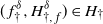 $(\,f^{\delta}_\dagger,H^{\delta}_{\dagger,\,f})\in H_\dagger$
. We will prove that there is a sequence
 $x_n\in E$
such that
 \begin{equation}\lim_{n\to \infty}u(x_n)-f^{\delta}_{\dagger}(x_n)=\sup\limits_{x\in E}u(x)-f^{\delta}_{\dagger}(x),\end{equation}
 \begin{equation}\limsup_{n\to\infty}u(x_n)-\lambda H^{\delta}_{\dagger,\,f}(x_n)-h(x_n)\leq 0.\end{equation}
As the function
 $[u-(1-\delta)f]$
is bounded from above and
 $\Upsilon$
has compact sublevel sets, the sequence
 $x_n$
along which the first limit is attained can be assumed to lie in the compact set
 \begin{equation*}K\,:\!=\, \bigl\{x\mid \Upsilon(x)\leq \delta^{-1}\sup\limits_{x}(u(x)-(1-\delta)\,f(x))\bigr\}.\end{equation*}
Set
 $M=\delta^{-1}\sup_{x}(u(x)-(1-\delta)\,f(x))$
. Let
 $\gamma\colon \mathbb{R}\to\mathbb{R}$
be a smooth increasing function such that
 \begin{equation*}\gamma(r)=\begin{cases}r &\text{if $r\leq M$,}\\M+1 &\text{if $r\geq M+2$.}\end{cases}\end{equation*}
Let
 $f_\delta$
be a function on E defined by
 \begin{equation*}f_{\delta}(x)\,:\!=\, \gamma((1-\delta)\,f(x)+\delta\Upsilon(x))=\gamma\big(\,f^{\delta}_\dagger(x)\big).\end{equation*}
By construction,
 $f_\delta$
is smooth and constant outside of a compact set and thus lies in
 $\mathcal{D}(H)=C^\infty_{cc}(E)$
. As u is a viscosity subsolution for
 $f-\lambda Hf=h$
, there exists a sequence
 $x_n\in K\subseteq E$
(by our choice of K) with
 \begin{gather}\lim_{n}u(x_n)-f_{\delta}(x_n)=\sup\limits_{x\in E}u(x)-f_{\delta}(x),\\[-38pt]\nonumber\end{gather}
 \begin{gather}\limsup_{n}u(x_n)-\lambda\mathbf{H}f_{\delta}(x_n)-h(x_n)\leq 0.\end{gather}
As
 $f_\delta$
equals
 $f^{\delta}_\dagger$
on K, we have from (5.7) that also
 \begin{equation*}\lim_{n}u(x_n)-f^{\delta}_\dagger(x_n)=\sup\limits_{x\in E}u(x)-f^{\delta}_\dagger(x),\end{equation*}
establishing (5.5). Convexity of
 $p\longmapsto\mathcal{H}(x,p)$
yields for arbitrary points
 $x\in K$
the estimate
 \begin{align*}\mathbf{H}f_\delta(x)&=\mathcal{H}(x,\partial_{x}f_\delta(x))\\ &\leq(1-\delta)\mathcal{H}(x,\partial_{x} \,f(x))+\delta\mathcal{H}(x,\partial_{x}\Upsilon(x))\\&\leq (1-\delta)\mathcal{H}(x,\partial_{x} \,f(x))+\delta C_\Upsilon\\ &=H^\delta_{\dagger,\,f}(x).\end{align*}
Combining this inequality with (5.8) yields
 \begin{align*}&\limsup_{n} u(x_n)-\lambda H^{\delta}_{\dagger,\,f}(x_n)-h(x_n)\\ &\quad \leq \limsup_{n}u(x_n)-\lambda \mathbf{H}f_\delta(x_n)-h(x_n)\\ &\quad \leq 0,\end{align*}
establishing (5.6). This concludes the proof.
Lemma 5.4. Fix
 $\lambda >0$
and
 $h\in C_b(E)$
.
-
(a) Every subsolution to
$f-\lambda Hf=h$
is also a subsolution to
$f-\lambda H_1f=h$
. -
(b) Every supersolution to
$f-\lambda Hf=h$
is also a supersolution to
$f-\lambda H_2f=h$
.


Proof. This proof has the same idea as Lemma 5.3, but we need to make appropriate modifications. To maintain integrity and readability, we give its proof in the following. We only prove part (a), as the proof of part (b) is similar.
Fix
 $\lambda >0$
and
 $h\in C_b(E)$
. Let u be a subsolution to
 $f-\lambda Hf=h$
. We prove that it is also a subsolution to
 $f-\lambda H_1f=h$
. Fix
 $\delta\in(0,1)$
,
 $\phi\in C^2_b(E\times S)$
and
 $f\in C_l^\infty(E)$
, such that
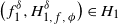 $\bigl(\,f^\delta_1,H^\delta_{1,\,f,\,\phi}\bigr)\in H_1$
. We will prove that there exist
 $(x_n,i_n)$
such that
 \begin{gather}\lim_{n}u(x_n)-f^{\delta}_1(x_n)=\sup\limits_{x}u(x)-f^{\delta}_1(x),\end{gather}
 \begin{gather}\limsup_{n}u(x_n)-\lambda H^\delta_{1,f,\phi}(x_n,i_n)-h(x_n)\leq 0.\end{gather}
We have that
 $M\,:\!=\, \delta^{-1}\sup_{x}(u(x)-(1-\delta)\,f(x))<\infty$
as u is bounded and
 $f\in C_l(E)$
. It follows that the sequence
 $x_n$
along which the limit in (5.9) is attained is contained in the compact set
 $K\,:\!=\, \{x\mid \Upsilon(x)\leq M\}$
.
Let
 $\gamma\colon \mathbb{R}\rightarrow\mathbb{R}$
be a smooth increasing function such that
 \begin{equation*}\gamma(r)=\begin{cases}r &\text{if $r\leq M$,}\\[5pt] M+1 &\text{if $r\geq M+2$.}\end{cases}\end{equation*}
Let
 $f_\delta$
denote the function on E defined by
 \begin{equation*}f_\delta(x)\,:\!=\, \gamma((1-\delta)\,f(x)+\delta\Upsilon(x))=\gamma\big(\,f^{\delta}_1(x)\big).\end{equation*}
By construction,
 $f_\delta$
is smooth and constant outside of a compact set and thus lies in
 $\mathcal{D}(H)=C^\infty_{cc}(E)$
. As
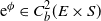 ${\mathrm{e}}^\phi\in C^2_b(E\times S)$
, we also have
 ${\mathrm{e}}^{(1-\delta)\phi}\in C^2(E\times S)$
. We conclude that
 $(\,f_\delta,H_{f_\delta,(1-\delta)\phi})\in H$
. As u is a viscosity subsolution for
 $f-\lambda Hf=h$
, there exist
 $x_n\in K\subseteq E$
(by our choice of K) and
 $i_n\in S$
with
 \begin{align}\lim_nu(x_n)-f_\delta(x_n)=\sup\limits_xu(x)-f_\delta(x), \end{align}
 \begin{align}\limsup_n u(x_n)-\lambda H_{f_\delta,(1-\delta)\phi}(x_n,i_n)-h(x_n)\leq 0.\end{align}
As
 $f_\delta$
equals
 $f^{\delta}_1$
on K, we have from (5.11) that also
 \begin{equation*}\lim_n u(x_n)-f^{\delta}_1(x_n)=\sup\limits_x u(x)-f^{\delta}_1(x),\end{equation*}
establishing (5.9). For arbitrary sequences
 $(x_n,i_n)$
, we have the elementary estimate
 \begin{align*}&H_{f_\delta,(1-\delta)\phi}(x_n,i_n)\\[5pt] &\quad =B_{x,\partial_{x}f_\delta(x)}(x_n,i_n)+{\mathrm{e}}^{-(1-\delta)\phi(x_n,i_n)}R_x{\mathrm{e}}^{(1-\delta)\phi(x_n,i_n)}\\[5pt] &\quad \leq (1-\delta)B_{x,\partial_{x}\,f(x)}(x_n,i_n)+\delta B_{x,\partial_{x}\Upsilon(x)}(x_n,i_n)+(1-\delta)\,{\mathrm{e}}^{-\phi(x_n,i_n)}R_x{\mathrm{e}}^{\phi(x_n,i_n)}\\[5pt] &\quad =(1-\delta)\bigl(B_{x,\partial_{x}\,f(x)}(x_n,i_n)+{\mathrm{e}}^{-\phi(x_n,i_n)}R_x{\mathrm{e}}^{\phi(x_n,i_n)} \bigr)+\delta B_{x,\partial_{x}\Upsilon(x)}(x_n,i_n)\\[5pt]&\quad \leq H^\delta_{1,f\!,\phi}(x_n,i_n).\end{align*}
In the first inequality, we use that
 $ B_{x,p}$
is convex concerning p. By virtue of (4.3), the last inequality holds. Combining the above inequality with (5.12) yields
 \begin{align*}&\limsup_n \bigl[u(x_n)-\lambda H^\delta_{1,f,\phi}(x_n,i_n)-h(x_n)\bigr]\\[5pt]&\quad \leq\limsup_n \bigl[u(x_n)-\lambda H_{f_\delta,\phi}(x_n,i_n)-h(x_n)\bigr]\\ &\quad \leq 0,\end{align*}
establishing (5.10). This concludes the proof.
Step 3: The comparison principle for
 $H_\dagger$
and
 $H_\ddagger$
.
The following lemma is to verify the comparison principle for Hamilton–Jacobi–Bellman equations involving the Hamiltonian
 $H_\dagger$
and
 $H_\ddagger$
.
Lemma 5.5. Assumptions 2.2 and 2.3 hold. Let
 $h_1$
,
 $h_2\in C_b(E)$
, and
 $\lambda>0$
. Let u be any subsolution to
 $f-\lambda H_{\dagger}f=h_1$
and let v be any supersolution to
 $f-\lambda H_{\ddagger}f=h_2$
. Then we have
 \begin{equation*}\sup\limits_{x}u(x)-v(x)\leq\sup\limits_{x}h_1(x)-h_2(x).\end{equation*}
The proof method of Lemma 5.5 adopts the doubling-of-variables technique, as described in [Reference Crandall, Ishii and Lions7]. This procedure requires selecting a suitable penalization function, while a more general definition can be found in Definition 5.2 of [Reference Kraaij20]. In our case, the chosen penalization function is the square of the distance
 \begin{equation} d^2(x,y)=\dfrac{2}{\theta^2}(\sqrt{x}-\sqrt{y})^2,\end{equation}
which fully utilizes the characteristics of the diffusion coefficient of CIR processes.
Before providing the proof of Lemma 5.5 we first state a lemma using the penalization function in (5.13), which helps us prove Lemma 5.5.
Lemma 5.6. (Lemma A.10 in [Reference Collet and Kraaij2].) Let u be bounded and upper semicontinuous, let v be bounded and lower semicontinuous, and let
 $\Upsilon$
be a good containment function in (4.1).
Fix
 $\delta>0$
. For every
 $m>0$
there exist points
 $x_{\delta,m}$
,
 $y_{\delta,m}\in E$
, such that
 \begin{align*}&\dfrac{u(x_{\delta,m})}{1-\delta}-\dfrac{v(y_{\delta,m})}{1+\delta}-md^2(x_{\delta,m},y_{\delta,m})-\dfrac{\delta}{1-\delta}\Upsilon(x_{\delta,m})-\dfrac{\delta}{1+\delta}\Upsilon(y_{\delta,m})\\ &\quad =\sup\limits_{x,y\in E}\biggl\{\dfrac{u(x)}{1-\delta}-\dfrac{v(y)}{1+\delta}-md^2(x,y)-\dfrac{\delta}{1-\delta}\Upsilon(x)-\dfrac{\delta}{1+\delta}\Upsilon(y)\biggr\}.\end{align*}
Additionally, for every
 $\delta>0$
we have the following.
-
(a) The set
$\{x_{\delta,m},y_{\delta,m} \mid m >0\}$
is relatively compact in E. -
(b) All limit points of
$\{(x_{\delta,m},y_{\delta,m})\}_{m >0}$
are of the form (z,z) and for these limit points we have
\begin{equation*} u(z)-v(z)=\sup\limits_{x\in E}u(x)-v(x).\end{equation*}
-
(c) We have
\begin{equation*}\lim_{m\to\infty}md^2(x_{\delta,m},y_{\delta,m})=0.\end{equation*}




Here we give the proof of Lemma 5.5.
Proof of Lemma 5.5. For
 $0<\delta<1$
and
 $m>1$
, let
 \begin{equation*}\Phi_{\delta,m}(x,y)\,:\!=\, \dfrac{u(x)}{1-\delta}-\dfrac{v(y)}{1+\delta}-md^2(x,y)-\dfrac{\delta}{1-\delta}\Upsilon(x)-\dfrac{\delta}{1+\delta}\Upsilon(y),\end{equation*}
where
 $d(\cdot,\cdot)$
is given in (5.13) and
 $\Upsilon(\!\cdot\!)$
is given in (4.1). Since
 $\Upsilon(\!\cdot\!)$
has compact level sets, there exists
 $(x_{\delta,m},y_{\delta,m})\in E\times E$
satisfying
 \begin{equation}\Phi_{\delta,m}(x_{\delta,m},y_{\delta,m})=\sup\limits_{(x,y)\in E\times E}\Phi_{\delta,m}(x,y).\end{equation}
Let
 $\varphi_1^{\delta,m}\in\mathcal{D}(H_\dagger)$
be defined as
 \begin{align*}\varphi_1^{\delta,m}(x)&\,:\!=\, (1-\delta)\bigg(\dfrac{v(y_{\delta,m})}{1+\delta}+md^2(x,y_{\delta,m})+\dfrac{\delta}{1-\delta}\Upsilon(x)+\dfrac{\delta}{1+\delta}\Upsilon(y_{\delta,m})\bigg) \\ &\quad+(1-\delta)(x-x_{\delta,m})^2,\end{align*}
where adding
 $(1-\delta)(x-x_{\delta,m})^2$
in
 $\varphi_1^{\delta,m}(x)$
implies that
 $u-\varphi_1^{\delta,m}$
attains its unique supremum at
 $x =x_{\delta,m}$
, namely
 \begin{align*}\sup\limits_{x\in E}u(x)-\varphi_1^{\delta,m}(x)=u(x_{\delta,m})-\varphi_1^{\delta,m}(x_{\delta,m}).\end{align*}
By the viscosity subsolution property of u, we have
 \begin{equation}u(x_{\delta,m})-\lambda\bigl[(1-\delta)\mathcal{H}\bigl(x_{\delta,m},p^1_{\delta,m}\bigr)+\delta C_{\Upsilon}\bigr]\leq h_1(x_{\delta,m}),\end{equation}
where
 \begin{equation} p^1_{\delta,m}\,:\!=\, m\partial_{x} d^2(x_{\delta,m},y_{\delta,m})=\dfrac{2m}{\theta^2}\bigg(1-\dfrac{\sqrt{y_{\delta,m}}}{\sqrt{x_{\delta,m}}}\bigg) .\end{equation}
Similarly, let
 $\varphi_2^{\delta,m}\in\mathcal{D}(H_\ddagger)$
be defined as
 \begin{align*}\varphi^{\delta,m}_2(y)&\,:\!=\, (1+\delta)\bigg(\dfrac{u(x_{\delta,m})}{1-\delta}-md^2(x,y_{\delta,m})-\dfrac{\delta}{1-\delta}\Upsilon(x_{\delta,m})-\dfrac{\delta}{1+\delta}\Upsilon(y)\bigg) \\ &\quad-(1+\delta)(y-y_{\delta,m})^2.\end{align*}
Therefore we obtain the supersolution inequality
 \begin{equation}v(x_{\delta,m})-\lambda\bigl[(1+\delta)\mathcal{H}\bigl(y_{\delta,m},p^2 _{\delta,m}\bigr)-\delta C_{\Upsilon}\bigr]\geq h_2(y_{\delta,m}),\end{equation}
where
 \begin{equation}p^2_{\delta,m}\,:\!=\, -m\partial_y d^2(x_{\delta,m},y_{\delta,m})=-\dfrac{2m}{\theta^2}\bigg(1-\dfrac{\sqrt{x_{\delta,m}}}{\sqrt{y_{\delta,m}}}\bigg) .\end{equation}
By Lemma 5.6, we have
 \begin{equation}\lim_{m\to\infty}md^2(x_{\delta,m},y_{\delta,m})=0.\end{equation}
Combining (5.15), (5.17), and (5.19), we get
 \begin{align} \sup\limits_{x\in E}u(x)-v(x)&\leq \liminf_{\delta\to0}\liminf_{m\to\infty}\bigg(\dfrac{u(x_{\delta,m})}{1-\delta}-\dfrac{v(y_{\delta,m})}{1+\delta}\bigg) \notag\\& \leq \liminf_{\delta\to0}\liminf_{m\to\infty}\biggl\{\dfrac{h_1(x_{\delta,m})}{1-\delta}-\dfrac{h_2(y_{\delta,m})}{1+\delta}\end{align}
 \begin{align}& \quad+\dfrac{\delta}{1-\delta}C_{\Upsilon}+\dfrac{\delta}{1+\delta}C_{\Upsilon}&\\& \quad+ \lambda\bigl(\mathcal{H}\bigl(x_{\delta,m},p^1_{\delta,m}\bigr)-\mathcal{H}\bigl(y_{\delta,m},p^2_{\delta,m}\bigr)\bigr)\biggr\},&\nonumber\end{align}
where in the first inequality we use (5.14) and drop the non-negative functions
 $d^2(\cdot,\cdot)$
and
 $\Upsilon(\!\cdot\!)$
. The term in (5.21) vanishes as
 $C_{\Upsilon}$
in (4.3) is a constant.
Based on Lemma 5.6, for fixed
 $\delta$
and varying m, the sequence
 $(x_{\delta,m},y_{\delta,m})$
takes its values in a compact set and hence admits converging subsequences. By Lemma 5.6(b), these subsequences converge to points of the form (x,x). Therefore we can deal with (5.20). Then, by the above analysis, we can get
 \begin{align*}\sup\limits_{x\in E}u(x)-v(x)&\leq \lambda\liminf_{\delta\to0}\liminf_{m\to\infty} \bigl(\mathcal{H}\bigl(x_{\delta,m},p^1_{\delta,m}\bigr)-\mathcal{H}\bigl(y_{\delta,m},p^2_{\delta,m}\bigr)\bigr)\\ &\quad+\sup\limits_{x\in E}h_1(x)-h_2(x).\end{align*}
It follows that the comparison principle holds for
 $f-\lambda H_\dagger f=h_1$
and
 $f-\lambda H_\ddagger f=h_2$
whenever, for any
 $\delta>0$
,
 \begin{equation} \liminf_{m\to\infty} \bigl(\mathcal{H}\bigl(x_{\delta,m},p^1_{\delta,m}\bigr)-\mathcal{H}\bigl(y_{\delta,m},p^2_{\delta,m}\bigr)\bigr)\leq0.\end{equation}
To that end, recall
 $\mathcal{H}(x,p)$
in (5.2):
 \begin{equation*}\mathcal{H}(x,p)=\sup\limits_{\pi\in\mathcal{P}(S)}\biggl\{\int B_{x,p}(z)\pi({\mathrm{d}} z)-\mathcal{I}(x,\pi)\biggr\},\end{equation*}
where
 $\pi\mapsto \int B_{x_{\delta,m},p^i_{\delta,m}}(z)\pi({\mathrm{d}} z)$
is bounded and continuous and
 $\mathcal{I}(x_{\delta,m},\cdot)$
has compact sublevel sets in
 $\mathcal{P}(S)$
. Thus there exists an optimizer
 $\pi_{\delta,m}\in\mathcal{P}(S)$
such that
 \begin{equation}\mathcal{H}\bigl(x_{\delta,m},p^1_{\delta,m}\bigr)=\int B_{x_{\delta,m},p^1_{\delta,m}}(z)\pi_{\delta,m}({\mathrm{d}} z)-\mathcal{I}(x_{\delta,m},\pi_{\delta,m})\end{equation}
and
 \begin{equation}\mathcal{H}\bigl(y_{\delta,m},p^2_{\delta,m}\bigr)\geq \int B_{x_{\delta,m},p^2_{\delta,m}}(z)\pi_{\delta,m}({\mathrm{d}} z)-\mathcal{I}(x_{\delta,m},\pi_{\delta,m}).\end{equation}
Combining (5.23) and (5.24), we obtain
 \begin{align}\mathcal{H}&\bigl(x_{\delta,m},p^1_{\delta,m}\bigr)-\mathcal{H}\bigl(y_{\delta,m},p^2_{\delta,m}\bigr)\notag\\ &\leq \int\bigl(B_{x_{\delta,m},p^1_{\delta,m}}(z)-B_{y_{\delta,m},p^2_{\delta,m}}(z)\bigr)\pi_{\delta,m}({\mathrm{d}} z)\end{align}
 \begin{align}&\quad+\mathcal{I}(y_{\delta,m},\pi_{\delta,m})-\mathcal{I}(x_{\delta,m},\pi_{\delta,m}).\end{align}
It is sufficient to prove that (5.25) and (5.26) are sufficiently small. For (5.25), by calculating the difference of integrand
 $B_{x,p}$
in detail, for any
 $z \in E$
and
 $i\in S$
, we have
 \begin{align*}&B_{x_{\delta,m},p^1_{\delta,m}}(z)-B_{y_{\delta,m},p^2_{\delta,m}}(z)\\ &\quad =\bigg(\eta(\mu(z)-x_{\delta,m})p^1_{\delta,m}+\dfrac{1}{2}\theta^2x_{\delta,m}(p^1_{\delta,m})^2\bigg) -\bigg(\eta(\mu(z)-y_{\delta,m})p^2_{\delta,m}+\dfrac{1}{2}\theta^2y_{\delta,m}(p^2_{\delta,m})^2\bigg) \\&\quad =\bigl(\eta(\mu(z)-x_{\delta,m})p^1_{\delta,m}-\eta(\mu(z)-y_{\delta,m})p^2_{\delta,m}\bigr)+\bigg(\dfrac{1}{2}\theta^2x_{\delta,m}(p^1_{\delta,m})^2- \dfrac{1}{2}\theta^2y_{\delta,m}(p^2_{\delta,m})^2 \bigg) \\&\quad =\dfrac{2m\eta}{\theta^2}(\mu(z)-y_{\delta,m})\bigg(1-\dfrac{\sqrt{x_{\delta,m}}}{\sqrt{y_{\delta,m}}}\bigg) +\dfrac{2m\eta}{\theta^2}(\mu(z)-x_{\delta,m})\bigg(1-\dfrac{\sqrt{y_{\delta,m}}}{\sqrt{x_{\delta,m}}}\bigg) \\&\quad =\dfrac{2m\eta}{\theta^2}\biggl[(\mu(z)-y_{\delta,m})\bigg(1-\dfrac{\sqrt{x_{\delta,m}}}{\sqrt{y_{\delta,m}}}\bigg) +(\mu(z)-x_{\delta,m})\bigg(1-\dfrac{\sqrt{y_{\delta,m}}}{\sqrt{x_{\delta,m}}}\bigg) \biggr]\\ &\quad =-m\eta\mu(z)\dfrac{d^2(x_{\delta,m},y_{\delta,m})}{\sqrt{x_{\delta,m}y_{\delta,m}}}-m\eta d^2(x_{\delta,m},y_{\delta,m})\leq 0,\end{align*}
where in the third equality we use (5.16) and (5.18). For (5.26), we utilize the equi-continuity of
 $\mathcal{I}(\cdot,\pi)$
established in Lemma 5.7 below for the spatial variable. We are left with stating and verifying Lemma 5.7. This finishes the proof of (5.22) and the comparison principle for
 $H_\dagger$
and
 $H_\ddagger$
.
Lemma 5.7. Let Assumptions 2.2 and 2.3 be satisfied. Recall (5.3):
 \begin{align*}\mathcal{I}(x,\pi)&=-\inf_{g>0}\int\dfrac{R_{x}g(z)}{g(z)}\pi({\mathrm{d}} z).\end{align*}
For any compact set
 $G\subseteq E$
and for all
 $\pi\in \mathcal{P}(S)$
, then
 $\{x\mapsto J(x,\pi)\}_{x\in G,\pi\in \mathcal{P}(S)}$
is uniformly continuous.
Proof. Let
 $\rho$
be some metric on the topology of E. We will prove that for any compact sets
 $G\subseteq E$
and
 $\varepsilon>0$
, there is some
 $\delta>0$
such that for all
 $x,y\in G$
with
 $\rho(x,y)\leq \delta$
and for all
 $\pi\in \mathcal{P}(S)$
, we have
 \begin{equation}|\mathcal{I}(x,\pi)-\mathcal{I}(y,\pi)|\leq \varepsilon.\end{equation}
By virtue of the definition of
 $\mathcal{I}$
, there exists a function
 $\phi\in C(S)$
independent of x such that
 ${\mathrm{e}}^\phi $
in the domain of
 $R_x$
, and
 \begin{align*}\mathcal{I}(x,\pi)&=-\inf_{g>0}\int\dfrac{R_{x}g(z)}{g(z)}\pi({\mathrm{d}} z)\\ &=\sup\limits_{\phi\in C(S)}\sum_{i,j\in S}q_{ij}(x)\pi_i\bigl(1-{\mathrm{e}}^{\phi(j)-{\phi(i)}}\bigr).\end{align*}
Let
 $x,y\in G$
. By continuity of the transition rate
 $q_{ij}(x)$
, the
 $\mathcal{I}(x,\cdot)$
are uniformly bounded for
 $x\in G$
:
 \begin{equation*}0\leq \mathcal{I}(x,\pi)\leq \sum_{i,j,i\neq j}q_{ij}(x)\pi_i\leq \sum_{i,j,i\neq j}q_{ij}(x)\leq \sum_{i,j,i\neq j}\bar{q}_{ij},\ \bar{q}_{ij}\,:\!=\, \sup\limits_{x\in G}q_{ij}(x).\end{equation*}
For any
 $n\in N$
, there exists
 $\phi^n\in C(S)$
such that
 \begin{equation*}0\leq \mathcal{I}(x,\pi)\leq \sum_{i,j,i\neq j}q_{ij}(x)\pi_i\bigl(1-{\mathrm{e}}^{\phi^n(j)-\phi^n(i)}\bigr)+\dfrac{1}{n}.\end{equation*}
By reorganizing, we find for all pairs (k,l) the bound
 \begin{equation*}\pi_k{\mathrm{e}}^{\phi^n(l)-\phi^n(k)}\leq \dfrac{1}{r_{G}(k,l)}\Bigg(\sum_{i,j,i\neq j}q_{ij}(x)\pi_i+\dfrac{1}{n}\Bigg) \leq \dfrac{1}{r_{G}(k,l)}\Bigg(\sum_{i,j,i\neq j}\bar{q}_{ij}+\dfrac{1}{n}\Bigg) ,\end{equation*}
where
 $r_{G}(k,l)\,:\!=\, \inf_{x\in G}q_{kl}(x)$
. Thereby, evaluating in
 $\mathcal{I}(y,\pi)$
the same function
 $\phi^n$
to estimate the supremum,
 \begin{align*}\mathcal{I}&(x,\pi)-\mathcal{I}(y,\pi)\\ &\leq\dfrac{1}{n}+\sum_{k,l,k\neq l}q_{kl}(x)\pi_k\bigl(1-{\mathrm{e}}^{\phi^n(l)}-{\mathrm{e}}^{\phi^n(k)}\bigr)-\sum_{k,l,k\neq l}q_{kl}(y)\pi_k\bigl(1-{\mathrm{e}}^{\phi^n(l)}-{\mathrm{e}}^{\phi^n(k)}\bigr)\\&\leq\dfrac{1}{n}+\sum_{k,l,k\neq l}|q_{kl}(x)-q_{kl}(y)|\pi_k+\sum_{k,l,k\neq l}|q_{kl}(y)-q_{kl}(x)|\pi_k {\mathrm{e}}^{\phi^n(l)-\phi^n(k)}\\ &\leq \dfrac{1}{n}+\sum_{k,l,k\neq l}|q_{kl}(x)-q_{kl}(y)|\Biggl[1+\dfrac{1}{r_{G}(k,l)}\Bigg(\sum_{k,l,k\neq l}\bar{q}_{kl}+1\Bigg) \Biggr].\end{align*}
We take
 $n\to \infty$
and use that the rates
 $x\mapsto q_{kl}(x)$
are Lipschitz-continuous under Assumption 2.3, and hence uniformly continuous on compact sets, to obtain (5.27). Hence the proof of the lemma is concluded.
6. Establishing the action-integral form of the rate function
In this section we start with the proof of Proposition 2.2(e),
 $V (t)f = \mathbf{V}(t)f$
; then we can re-express the rate function (2.10). We first give the strategy to prove
 $V (t)f = \mathbf{V}(t)f$
in our context. Recall that the resolvent is given by
 \begin{equation*}\mathbf{R}(\lambda)h(x)=\sup\limits_{\substack{\gamma\in\mathcal{AC}\\ \gamma(0)=x}}\int^\infty_0\lambda^{-1}{\mathrm{e}}^{-\lambda^{-1}t}\bigg(h(\gamma(t))-\int^t_0\mathcal{L}(\gamma(s),\dot{\gamma}(s))\,{\mathrm{d}} s\bigg) \,{\mathrm{d}} t.\end{equation*}
If Conditions 8.9, 8.10, and 8.11 in [Reference Feng and Kurtz14] hold, which are modified as Condition 6.1 below, adapted to our setting, we obtain the following important results.
-
• For
$\lambda>0$
we have
$\mathbf{R}(\lambda)C_b(E)\subseteq C_b(E)$
, and
$\mathbf{R}(\lambda)h$
is a viscosity solution of
$f-\lambda \mathbf{H}f=h$
, following the first part of the proof of [Reference Feng and Kurtz14, Theorem 8.27]. -
• For
$f \in C_b(E)$
, (6.1)thanks to [Reference Feng and Kurtz14, Lemma 8.18].
\begin{equation} \lim_{n\to\infty}\|\mathbf{V}(t)f-\mathbf{R}(t/n)^{n}f\|=0,\end{equation}




Subsequently, by the comparison principle, we first have
 $\mathbf{R}(\lambda)h=R(\lambda)h$
,
 $h\in C_b(E)$
. Then, by (6.1) and (2.9), we get
 $V(t)f=\mathbf{V}(t)f$
,
 $f\in C_b(E)$
, and the action-integral representation form (2.12). We are left to modify Conditions 8.9, 8.10, and 8.11 adapted to our setting.
Condition 6.1. Let
 $\mathcal{H}\colon E\times \mathbb{R}\to \mathbb{R}$
be the map defined in (5.2). For any
 $f\in C^\infty_b(E)$
,
 $\mathbf{H}\,f(x)=\mathcal{H}(x,\partial_x \,f(x))$
. Assume that for any
 $(x,v)\in E\times \mathbb{R}$
,
 $\mathcal{H}(x,v)$
is continuous and convex in the second variable v. Let
 $\mathcal{L}$
denote the Legendre transform of
 $\mathcal{H}$
. Furthermore, suppose that there exists a good containment function
 $\Upsilon$
for
 $\mathcal{H}$
.
Then the following hold.
-
(a) The function
$\mathcal{L}\colon E\times \mathbb{R} \to [0,\infty]$
is lower semicontinuous, and for each compact set
$K\subseteq E$
and for
$c \in \mathbb{R}$
, the level set is relatively compact.
\begin{equation*} \{ (x, v)\in E\times \mathbb{R} \mid x\in K, \mathcal{L}(x, v)\leq c \}\end{equation*}
-
(b) For each compact set
$K\subseteq E$
,
$T>0$
, and
$0\leq C<\infty$
, there exists a compact set
$\tilde{K}=\tilde{K}(K,T,C)\subseteq E$
such that for any absolutely continuous path
$\gamma\colon [0,T]\to E$
with
$\gamma(0)\in K$
and implies
\begin{equation*} \int^T_0\mathcal{L}(\gamma(t),\dot{\gamma}(t))\,{\mathrm{d}} t\leq C\end{equation*}
$\gamma(t)\in \tilde{K}$
for all
$0\leq t\leq T$
.
-
(c) For each
$f\in C_c(E)$
and compact
$K\subseteq E$
, there exists a right continuous non-decreasing function
$\psi_{f,K}\colon [0,\infty)\to [0,\infty)$
such that and
\begin{equation*} \lim_{r\to \infty}r^{-1}\psi_{f,K}(r)=0\end{equation*}
\begin{equation*} |\partial_x \,f(x)\cdot v|\leq \psi_{f,K}(\mathcal{L}(x,v)) \quad for\ all\ \text{$(x,v)\in K \times \mathbb{R}$.}\end{equation*}
-
(d) For each
$x_0\in E$
and every
$f \in \mathcal{D}(\mathbf{H})$
, there exists an absolutely continuous path
$x\colon [0,\infty) \mapsto E$
such that
$x(0)=x_0$
, and for any
$t\geq 0$
,
\begin{equation*} \int^t_0 \mathcal{H}(x(s),\partial_x\,f(x(s))))\,{\mathrm{d}} s = \int^t_0 \partial_x\,f(x(s)) \cdot \dot{\!x}(s)-\mathcal{L}(x(s),\dot{\!x}(s))] \,{\mathrm{d}} s .\end{equation*}












Proof of Condition 6.1. In fact we extend the condition appearing in the proof of Proposition 6.1 in [Reference Peletier and Schlottke24] to the non-compact setting by combining Section 4 of [Reference Kraaij and Schlottke23]. For the proof of (a), (c), and (d), we refer to [Reference Peletier and Schlottke24], but with attention to the compact set. For the proof of (b), we refer to [Reference Kraaij and Schlottke23]. Now Condition 6.1 immediately follows.
Using Condition 6.1, we obtain the following proposition.
Proposition 6.1. For any
 $f \in C_b(E)$
, under Condition 6.1, the rate function (2.10) can be re-expressed in action-integral form as in (2.12).
To prove Proposition 6.1, we need the following two lemmas.
Lemma 6.1. Under Condition 6.1, for any
 $f\in C_b(E)$
, then
 $\mathbf{V}(t)f=V(t)f$
.
The proof of Lemma 6.1 follows from the analytical discussion at the beginning of this section.
Lemma 6.2. Let
 $x\colon [0,T]\to E$
be absolutely continuous curves. Under Condition 6.1, it yields that
 \begin{equation} I^V_{t_1-t_0}(x(t_1)\mid x(t_0))=\inf_{\substack{\gamma(t_0)=x(t_0)\\ \gamma(t_1)=x(t_1)}}\int^t_0 \mathcal{L}(\gamma(s),\dot{\gamma}(s))\,{\mathrm{d}} s, \end{equation}
where the infimum is taken over absolutely continuous paths
 $\gamma\colon [t_0, t_1 ] \to E$
.
The proof of Lemma 6.2 is rather lengthy. To ensure clarity in the main line of reasoning, we defer its proof to the end of this section.
Having made this arrangement, the lemmas and conditions established above provide the necessary foundation for proving Proposition 6.1.
Proof of Proposition 6.1
. By the result of Lemma 6.2, for arbitrary
 $k\in \mathbb{N}$
and points in time
 $0= t_0,t_1,\ldots, t_k = T$
we obtain the estimate
 \begin{equation*} I^V_{t_1-t_0}(x(t_1)\mid x(t_0))+I^V_{t_2-t_1}(x(t_2)\mid x(t_1))+\cdots+I^V_{t_k-t_{k-1}}(x(t_k)\mid x(t_{k-1})\leq \int^T_0\mathcal{L}(x(s),\dot{\!x}(s))\,{\mathrm{d}} s,\end{equation*}
since
 $x(\!\cdot\!)$
satisfies the start- and end-point constraints. For the reverse inequality, we note that adding time points increases the two-point rate functions since we add a condition on the paths; for
 $t_0 < t_1 < t_2 $
,
 \begin{align*} &{I}^V_{t_2-t_0}(x(t_2)\mid x(t_0))\\ &\quad=\inf_{\substack{\gamma(t_0)=x(t_0)\\ \gamma(t_2)=x(t_2)}}\biggl[\int^{t_1}_{t_0}\mathcal{L}(\gamma(s),\dot{\gamma}(s))\,{\mathrm{d}} s+\int^{t_2}_{t_1}\mathcal{L}(\gamma(s),\dot{\gamma}(s))\,{\mathrm{d}} s\biggr]\\ &\quad\leq \inf_{\substack{\gamma(t_0)=x(t_0)\\ \gamma(t_1)=x(t_1)}}\biggl[\int^{t_1}_{t_0}\mathcal{L}(\gamma(s),\dot{\gamma}(s))\,{\mathrm{d}} s\biggr]+\inf_{\substack{\gamma(t_1)=x(t_1)\\ \gamma(t_2)=x(t_2))}}\biggl[\int^{t_2}_{t_1}\mathcal{L}(\gamma(s),\dot{\gamma}(s))\,{\mathrm{d}} s\biggr]\\ &\quad={I}^V_{t_2-t_1}(x(t_2)\mid x(t_1))+{I}^V_{t_1-t_0}(x(t_1)\mid x(t_0)).\end{align*}
The partitions of a time interval [0, T] give rise to a monotonically increasing sequence. As in [Reference Villani27, Definition 7.11, Example 7.12], we obtain
 \begin{equation*}\sup\limits_k\sup\limits_{t_i}\sum^k_{i=0}{I}^V_{t_{i+1}-t_{i}}(x(t_{i+1})\mid x(t_{i}))=\int^T_0\mathcal{L}(x(s),\dot{\!x}(s))\,{\mathrm{d}} s.\end{equation*}
The proof of Proposition 6.1 is complete.
Proof of Lemma 6.2. We first prepare to express
 $I^V_{t_1-t_0}$
. To this end, for
 $f\in C_b(E)$
and
 $x(t_0)\in E$
, by Lemma 6.1 we obtain
 \begin{align}V(t_1)\,f(x(t_0))&=\mathbf{V}(t_1)\,f(x(t_0)) \notag \\ &=\sup\limits_{\gamma(t_0)=x(t_0)}\biggl\{\,f(\gamma(t_1))-\int^{t_1}_{t_0}\mathcal{L}(\gamma(s),\dot{\gamma}(s))\,{\mathrm{d}} s\biggr\} \notag \\ &=-\inf_{\gamma(t_0)=x(t_0)}\biggl\{\int^{t_1}_{t_0}\mathcal{L}(\gamma(s),\dot{\gamma}(s))\,{\mathrm{d}} s-\,f(\gamma(t_1))\biggr\},\end{align}
where the second equality follows from the definition of the Nisio semigroup. Next, combining (2.11) with (6.3), we have
 \begin{align}&I^V_{t_1-t_0}(x(t_1)\mid x(t_0)) \notag \\ &\quad =\sup\limits_{f\in C_b(E)}(\,f(x(t_1))-\mathbf{V}(t_1)\,f(x(t_0))) \notag\\ &\quad =\sup\limits_{f\in C_b(E)}\inf_{\gamma(t_0)=x(t_0)}\biggl[\,f(x(t_1))-\,f(\gamma(t_1))+\int^{t_1}_{t_0}\mathcal{L}(\gamma(s),\dot{\gamma}(s)\,{\mathrm{d}} s\biggr]. \end{align}
To establish (6.2), from (6.4), it suffices to show
 \begin{align} &\sup\limits_{f\in C_b(E)}\inf_{\gamma(t_0)=x(t_0)}\biggl[\,f(x(t_1))-\,f(\gamma(t_1))+\int^{t_1}_{t_0}\mathcal{L}(\gamma(s),\dot{\gamma}(s)\,{\mathrm{d}} s\biggr] \notag \\ &\quad\leq \inf_{\substack{\gamma(t_0)=x(t_0)\\ \gamma(t_1)=x(t_1)}}\int^t_0 \mathcal{L}(\gamma(s),\dot{\gamma}(s))\,{\mathrm{d}} s \end{align}
and
 \begin{align} &\sup\limits_{f\in C_b(E)}\inf_{\gamma(t_0)=x(t_0)}\biggl[\,f(x(t_1))-\,f(\gamma(t_1))+\int^{t_1}_{t_0}\mathcal{L}(\gamma(s),\dot{\gamma}(s)\,{\mathrm{d}} s\biggr] \notag \\ & \quad\geq \inf_{\substack{\gamma(t_0)=x(t_0)\\ \gamma(t_1)=x(t_1)}}\int^t_0 \mathcal{L}(\gamma(s),\dot{\gamma}(s))\,{\mathrm{d}} s. \end{align}
Proof of (6.5): for any
 $f\in C_b(E)$
, since the set of curves
 $\{\gamma\colon \gamma(t_0)=x(t_0)\}$
contains its subset
 $\{\gamma \colon \gamma(t_0)=x(t_0),\gamma(t_1)=x(t_1)\}$
, we obtain the inequality
 \begin{equation*} \inf_{\gamma(t_0)=x(t_0)}\biggl[\,f(x(t_1))-\,f(\gamma(t_1))+\int^{t_1}_{t_0}\mathcal{L}(\gamma(s),\dot{\gamma}(s)\,{\mathrm{d}} s\biggr]\leq \inf_{\substack{\gamma(t_0)=x(t_0)\\ \gamma(t_1)=x(t_1)}}\int^{t_1}_{t_0}\mathcal{L}(\gamma(s),\dot{\gamma}(s)\,{\mathrm{d}} s. \end{equation*}
Furthermore, taking the supremum over all
 $f\in C_b(E)$
, the inclusion relation between the path sets remains valid, and the inequality still holds. Thus we arrive at (6.5).
Proof of (6.6): based on the definition of supremum, for any
 $f\in C_b(E)$
, we have
 \begin{align} &\sup\limits_{f\in C_b(E)}\inf_{\gamma(t_0)=x(t_0)}\biggl[\,f(x(t_1))-\,f(\gamma(t_1))+\int^{t_1}_{t_0}\mathcal{L}(\gamma(s),\dot{\gamma}(s)\,{\mathrm{d}} s\biggr] \notag \\ &\quad\geq \inf_{\gamma(t_0)=x(t_0)}\biggl[\,f(x(t_1))-\,f(\gamma(t_1))+\int^{t_1}_{t_0}\mathcal{L}(\gamma(s),\dot{\gamma}(s)\,{\mathrm{d}} s\biggr]. \end{align}
Then, according to the definition of infimum, for any
 $m>0$
, there exist curves
 $\gamma_m$
satisfying
 $\gamma_m(t_0)=x(t_0)$
such that
 \begin{align} &\inf_{\gamma(t_0)=x(t_0)}\biggl[\,f(x(t_1))-\,f(\gamma(t_1))+\int^{t_1}_{t_0}\mathcal{L}(\gamma(s),\dot{\gamma}(s)\,{\mathrm{d}} s\biggr]\notag \\ &\quad\geq \,f(x(t_1))-\,f(\gamma_m(t_1))+\int^{t_1}_{t_0}\mathcal{L}(\gamma_m(s),\dot{\gamma}_m(s))\,{\mathrm{d}} s-\dfrac{1}{m}.\end{align}
From (6.4), (6.7), and (6.8), we get
 \begin{align} & I^V_{t_1-t_0}(x(t_1)\mid x(t_0)) \notag\\ &\quad= \sup\limits_{f\in C_b(E)}\inf_{\gamma(t_0)=x(t_0)}\biggl[\,f(x(t_1))-\,f(\gamma(t_1))+\int^{t_1}_{t_0}\mathcal{L}(\gamma(s),\dot{\gamma}(s)\,{\mathrm{d}} s\biggr]\notag \\ &\quad\geq \,f(x(t_1))-\,f(\gamma_m(t_1))+\int^{t_1}_{t_0}\mathcal{L}(\gamma_m(s),\dot{\gamma}_m(s))\,{\mathrm{d}} s-\dfrac{1}{m}.\end{align}
Either
 $I^V_{t_1-t_0}(x(t_1)\mid x(t_0))=\infty$
or there exists a sequence
 $x_m$
such that
 $x_m(t_1)\to \gamma_m(t_1)$
and
 \[\limsup_{m\to \infty}\int^{t_1}_{t_0}\mathcal{L}(\gamma_m(s),\dot{\gamma}_m(s))\,{\mathrm{d}} s<\infty.\]
Then, using Condition 6.1(b), we conclude that
 $\gamma_m$
lies in a compact set. Therefore there exists a converging subsequence of
 $\gamma_m$
(also denoted by
 $\gamma_m$
).
-
(i) If
$\gamma_m(t_1)\nrightarrow x(t_1)$
, then
$I^V_t(x(t_1)\mid x(t_0))=\infty$
, and (6.6) holds. -
(ii) If
$\gamma_m(t_1)\to x(t_1)$
, by continuity of f, lower semicontinuity of
$\gamma\mapsto \int^{t_1}_{t_0}\mathcal{L}(\gamma(s),\dot{\gamma}(s)\,{\mathrm{d}} s$
, and the definition of infimum, from (6.9) we havewhere
\begin{align*}&\sup\limits_{f\in C_b(E)}\inf_{\gamma(t_0)=x(t_0)}\biggl[\,f(x(t_1))-\,f(\gamma(t_1))+\int^{t_1}_{t_0}\mathcal{L}(\gamma(s),\dot{\gamma}(s)\,{\mathrm{d}} s\biggr] \\ &\quad\geq \liminf_{m\to \infty}\biggl[\,f(x(t_1))-\,f(\gamma_m(t_1))+\int^{t_1}_{t_0}\mathcal{L}(\gamma_m(s),\dot{\gamma}_m(s))\,{\mathrm{d}} s\biggr] \\&\quad\geq \int^{t_1}_{t_0}\mathcal{L}(\gamma(s),\dot{\gamma}(s)\,{\mathrm{d}} s\\ &\quad \geq \inf_{\substack{\gamma(t_0)=x(t_0) \\ \gamma(t_1)=x(t_1)}}\int^{t_1}_{t_0}\mathcal{L}(\gamma(s),\dot{\gamma}(s)\,{\mathrm{d}} s, \end{align*}
$\gamma$
represents an absolutely continuous path.






7. Proof of existence and uniqueness
In order to prove Proposition 2.1, we use the methods of Skorokhod’s representation and pathwise splicing. In the following, we start by introducing Skorokhod’s representation of the fast process
 $\Lambda^\varepsilon_n(t)$
.
7.1. Skorokhod’s representation
The role of Skorokhod’s representation is to represent the evolution of the discrete component
 $\Lambda^{\varepsilon}_n(t)$
in the form of a stochastic integral with respect to a Poisson random measure (see e.g. [Reference Shao25]). Precisely, for each
 $x\in E$
, construct a family of disjoint intervals
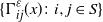 $\{ \Gamma^{\varepsilon}_{ij}(x)\colon i,j\in S \}$
on the positive half real line
 $\mathbb{R}^+$
in the following manner:
 \begin{align*}\Gamma^{\varepsilon}_{12}(x)&=\biggl[0,\ \dfrac{1}{\varepsilon}q_{12}(x)\bigg) \\\Gamma^{\varepsilon}_{13}(x)&=\biggl[\dfrac{1}{\varepsilon}q_{12}(x),\ \dfrac{1}{\varepsilon}[q_{12}(x)+q_{13}(x)]\bigg) \\&\ \vdots\\\Gamma^{\varepsilon}_{1N}(x)&=\Biggl[\dfrac{1}{\varepsilon}\sum_{j=1}^{N-1}q_{1j}(x),\ \dfrac{1}{\varepsilon}q_1(x)\Bigg) \\\Gamma^{\varepsilon}_{21}(x)&=\biggl[\dfrac{1}{\varepsilon}q_1(x),\ \dfrac{1}{\varepsilon}[q_1(x)+q_{21}(x)]\bigg) \\\Gamma^{\varepsilon}_{23}(x)&=\biggl[\dfrac{1}{\varepsilon}[q_1(x)+q_{21}(x)],\ \dfrac{1}{\varepsilon}[q_1(x)+q_{21}(x)+q_{23}(x)]\bigg)\\&\ \vdots\end{align*}
and so on. Therefore we obtain a sequence of consecutive, left-closed, right-open intervals
 $\Gamma^{\varepsilon}_{ij}(x)$
of
 $\mathbb{R}^+$
, each having length
 ${\frac{1}{\varepsilon}}q_{ij}(x)$
. For convenience of notation, we set
 $\Gamma^{\varepsilon}_{ii}(x)= \emptyset$
and
 $\Gamma^{\varepsilon}_{ij}(x)=\emptyset$
if
 $q_{ij}(x)=0$
,
 $i\neq j$
.
Define a function
 $h^{\varepsilon}\colon E\times S \times M^{\varepsilon}\rightarrow\mathbb{R}$
by
 \begin{equation*}h^{\varepsilon}(x,i,z)=\sum_{l\in S}(l-i)\mathbf{1}_{{\Gamma}^{\varepsilon}_{il}(x)}(z).\end{equation*}
Thus, given the partition
 \[\{\Gamma^{\varepsilon}_{ij}(x)\colon i,j\in S\ \text{with $i\neq j$}\},\]
and for each
 $i\in S$
, if
 $z\in \Gamma^\varepsilon_{ij}(x)$
,
 $h^{\varepsilon}(x,i,z)=j-i$
; otherwise
 $h^{\varepsilon}(x, i, z) = 0$
. By [Reference Skorokhod26, Section II-2.1], the evolution of the transition probabilities (2.2) can be described by the evolution of states as follows:
 \begin{equation}{\mathrm{d}} \Lambda^{\varepsilon}_n (t) = \int_{[0,M^{\varepsilon}]}h^\varepsilon(X^\varepsilon_n(t),\Lambda^{\varepsilon}(t-),z)N({\mathrm{d}} t,{\mathrm{d}} z),\end{equation}
where
 $M^{\varepsilon} = N (N - 1)H^{\varepsilon}$
with
 \[H^{\varepsilon}\,:\!=\, \max_{i,j\in S}\sup\limits_{x\in \mathbb{R}}\frac{1}{\varepsilon}q_{ij}(x)<\infty.\]
 $N({\mathrm{d}} t,{\mathrm{d}} z)$
is a Poisson random measure(corresponding to a stationary point process p(t)) with intensity
 ${\mathrm{d}} t \times \mathbf{m}({\mathrm{d}} z)$
, and
 $\mathbf{m}({\mathrm{d}} z)$
is the Lebesgue measure on
 $[0,M^{\varepsilon}]$
. Note that
 $N(\cdot,\cdot)$
does not depend on
 $\varepsilon$
, because the function
 $h^{\varepsilon}(\cdot,\cdot,\cdot)$
contains all information about
 ${\frac{1}{\varepsilon}}q(\!\cdot\!)$
; see [Reference Xi and Zhu28, Proposition 2.4].
 $N(\cdot,\cdot)$
is independent of the Brownian motion
 $W(\!\cdot\!)$
. Due to the finiteness of
 $\mathbf{m}(\!\cdot\!)$
on
 $[0, M^{\varepsilon}]$
, there is only a finite number of jumps of the process p(t) in each finite time interval. Let
 $\sigma_1<\sigma_2<\ldots<\ldots$
be the enumeration of all elements in the domain
 $D_{p}$
of the stationary point process p(t) corresponding to the above Poisson random measure
 $N({\mathrm{d}} t,{\mathrm{d}} z)$
. It follows that
 $\lim_{n\to\infty}\sigma_n=\infty$
almost surely.
Remark 7.1. Equation (2.2) describes the evolution of the jump process, but it is difficult to study the existence and uniqueness of the solution directly by using (2.2). Skorokhod’s representation is a good method to express (2.2) with the integral equation, and the information contained is not lost.
7.2 Proof of Proposition 2.1
For each
 $k\in S$
, once we have fixed a state, (2.1) becomes a classical CIR process
 \begin{equation}{\mathrm{d}} X^{\varepsilon,(k)}_n(t)=\eta(\mu(k)-X^{\varepsilon,(k)}_n(t))\,{\mathrm{d}} t+n^{-{{1}/{2}}}\theta\sqrt{X^{\varepsilon,(k)}_n(t)}\,{\mathrm{d}} W(t).\end{equation}
There exists a unique non-negative strong solution of (7.2) with
 $2\eta u(k)\geq \theta^2$
due to [Reference Karatzas and Shreve19, Proposition 5.2.13 and Corollary 5.3.23] by the Yamada–Watanabe theorem.
Proof of Proposition 2.1. The idea of the proof comes from the stationarity of Brownian motion and the Poisson point process, and we segment the path space via stopping times; see Figure 2.
The time interval.

Step 1. Let us first consider the solution in the time interval
 $[0,\sigma_1]$
, where
 $\sigma_1$
is the stopping time. For any
 $t\in [0,\sigma_1)$
and any path
 $\{ (X^{\varepsilon}_n(s),\Lambda^{\varepsilon}_n(s))\colon 0\leq s\leq t\}$
, we always have
 \begin{equation*}\int^t_0\int_{[0,M^{\varepsilon}]}h^\varepsilon(X^{\varepsilon}_n(s-),\Lambda^{\varepsilon}_n(s-),z)N({\mathrm{d}} s,{\mathrm{d}} z)\equiv0, \quad\text{and then} \ \Lambda^{\varepsilon}_n(t)\equiv\Lambda^{\varepsilon}_n(0)=k.\end{equation*}
Hence, on the interval
 $[0,\sigma_1)$
, (2.1) is equivalent to (7.2), which has a unique strong solution
 $X^{\varepsilon,(k)}_n(t)$
with
 $X^{\varepsilon,(k)}_n(0)=x$
, so
 \[\big(X^{\varepsilon}_n(t),\Lambda^{\varepsilon}_n(t)\big)=\bigl(X^{\varepsilon,(k)}_n(t),k\bigr)\quad\text{for $0\leq t<\sigma_1$.}\]
From (7.1) we have
 \begin{equation*}\Lambda^{\varepsilon}_n(\sigma_1)=k+\sum_{l\in S}(l-k)\mathbf{1}_{\Gamma^{\varepsilon}_{kl}(X^{\varepsilon,(k)}_n(\sigma_1))}(p(\sigma_1)).\end{equation*}
Then, on the time interval
 $[0,\sigma_1]$
, set
 \begin{equation}\big(X^{\varepsilon}_n(t),\Lambda^{\varepsilon}_n(t)\big)=\begin{cases}\big(X^{\varepsilon,(k)}_n(t),k\big), & 0\leq t<\sigma_1,\\\big(X^{\varepsilon,(k)}_n(\sigma_1),\Lambda^{\varepsilon}_n(\sigma_1)\big), & t=\sigma_1.\end{cases}\end{equation}
Next, set
 $\tilde{\xi}=X^{\varepsilon}_n(\sigma_1)$
,
 $\tilde{W}(t)=W(t+\sigma)-W(t)$
, and
 $\tilde{p}(t)=p(t+\sigma_1)$
.
Step 2. Similarly, we consider the solution on the interval
 $[0,\sigma_2-\sigma_1]$
with respect to
 $(\tilde{\xi},\Lambda^{\varepsilon}_n(\sigma_1))$
as above, and define
 \begin{align*}\big(\tilde{X}^{\varepsilon}_n(t),\tilde{\Lambda}^{\varepsilon}_n(t)\big) & =\bigl(X^{\varepsilon,(\Lambda^{\varepsilon}_n(\sigma_1))}_n(t),\Lambda^{\varepsilon}_n(\sigma_1)\bigr)\quad \text{for $0\leq t<\sigma_2-\sigma_1$,}\\\tilde{X}^{\varepsilon}_n(\sigma_2-\sigma_1) & =X^{\varepsilon,(\Lambda^{\varepsilon}(\sigma_1))}_n(\sigma_2-\sigma_1),\\\tilde{\Lambda}^{\varepsilon}_n(\sigma_2-\sigma_1) & =\Lambda^{\varepsilon}_n(\sigma_1)+\sum_{l\in S}\big(l-\Lambda^{\varepsilon}_n(\sigma_1)\big)\textbf{1}_{\tilde{A}^{\varepsilon}_n(l)}(\tilde{p}(\sigma_2-\sigma_1)),\end{align*}
where
 \begin{equation*}{\tilde{A}^{\varepsilon}_n(l)=\Gamma^{\varepsilon}_{\Lambda^{\varepsilon}_n(\sigma_1)l}\bigl(X^{\varepsilon,(\Lambda^\varepsilon_n(\sigma_1))}_n(\sigma_2-\sigma_1)\bigr).}\end{equation*}
Furthermore, we define
 \begin{equation*}\big(X^{\varepsilon}_n(t),\Lambda^{\varepsilon}_n(t)\big)=\big(\tilde{X}^{\varepsilon}_n(t-\sigma_1),\tilde{\Lambda}^{\varepsilon}_n(t-\sigma_1)\big),\quad t\in[\sigma_1,\sigma_2],\end{equation*}
which together with (7.3) gives the solution on the time interval
 $[0,\sigma_2]$
. Continuing this procedure inductively,
 $(X^{\varepsilon}_n(t),\Lambda^{\varepsilon}_n(t))$
is determined uniquely on the time interval
 $[0,\sigma_n]$
for every n, and thus
 $(X^{\varepsilon}_n(t),\Lambda^{\varepsilon}_n(t))$
is determined globally because
 $\lim_{n\to\infty}\sigma_n=\infty$
almost surely.
Step 3. Consequently, we have proved the existence of a unique strong solution to the systems (2.1) and (7.1).
The proof is complete.
Appendix A. Nonlinear semigroup methods
In this paper the proof of Theorem 2.1 is originally based on the ideas presented by Feng and Kurtz [Reference Feng and Kurtz14]. The key idea of the method is to establish the convergence of semigroups, which is referred to as the nonlinear semigroup method. Many theorems and lemmas are involved in the proof. After analysis, we focus on verifying assumptions (a)–(e) in Proposition 2.2 to establish Theorem 2.1. Here we further explain why assumptions (a)–(e) in Proposition 2.2 can be used to prove the large deviation principle via the following three steps.
Step 1. For the Markov process
 $(X_n(t), \Lambda_n(t))$
, we aim to prove the LDP on the path space. The approach is based on a variant of the projective limit theorem, [Reference Feng and Kurtz14, Theorem 4.28]. It suffices to prove exponential tightness and the LDP for the finite-dimensional distributions. Then we obtain the LDP, and the rate function is given in the projective limit form: the supremum over the rate functions of the finite-dimensional distributions.
Step 2. The exponential tightness of the Markov process is proposed as an assumption in Proposition 2.2(c).
For the LDP of the finite-dimensional distributions, we first consider
 $k=0$
with
 $f_0\in C_b(E\times S)$
and
 $t_0=0$
. The LDP for
 $X_n(t_0)$
with rate function
 $I_0$
is assumed in Proposition 2.2(a). By the Varadhan theorem [Reference Dembo and Zeitouni8, Theorem 4.3.1], for
 $X_n(t_0)$
, we have
 \begin{equation} \lim_{n\to \infty}\dfrac{1}{n}\log \mathbb{E}\bigl[{\mathrm{e}}^{nf_0(x_0,k_0)}\bigr]=\sup\limits_{z}\,\{f_0(z)-I_0(z)\}.\end{equation}
For
 $k=0, 1$
with
 $f_0$
,
 $f_1\in C_b(E\times S)$
and
 $0=t_0<t_1$
, we have
 \begin{align*}&\Gamma_n \nonumber (t_0,t_1)(\,f_0,f_1)\\ \nonumber &\quad \,:\!=\, \dfrac{1}{n}\log\mathbb{E}\bigl({\mathrm{e}}^{n f_0(X_n(t_0),\Lambda_n(t_0))+n f_1(X_n(t_1),\Lambda_n(t_1))}\bigr)\\ \nonumber&\quad =\dfrac{1}{n}\log \mathbb{E}\bigl[\mathbb{E}\bigl({\mathrm{e}}^{n f_0(X_n(t_0),\Lambda_n(t_0))+n f_1(X_n(t_1),\Lambda_n(t_1))}\mid (X_n(t_0),\Lambda_n(t_0))=(x_0,k_0)\bigr)\bigr]\\&\quad =\dfrac{1}{n}\log \mathbb{E}\bigl({\mathrm{e}}^{n f_0(x_0,k_0)+n V_n(t_1) f_1(x_0,k_0)} \bigr)\\ \nonumber &\quad =\dfrac{1}{n}\log\mathbb{E}\bigl({\mathrm{e}}^{nf_0(x_0,k_0)}\bigr)+\dfrac{1}{n}\mathbb{E}\bigl({\mathrm{e}}^{n V_n(t_1) f_1(x_0,k_0)}\bigr)\\ &\quad -\!: \Gamma_{n,0}(t_0)f_0+\Gamma_{n,1}(t_1)f_1,\nonumber\end{align*}
where in the third equality we used the Markov property and the conditional log-Laplace transform
 $V_n(t_1)$
as defined in (2.6).
We aim to get the limit of
 $\Gamma_n(t_0,t_1)(\,f_0,f_1)$
for proving the LDP of
 $(X_n(t_0),X_n(t_1))$
by the Bryc theorem [Reference Dembo and Zeitouni8, Theorem 4.4.2]. To this end, by (A.1), we first have
 \begin{equation}\lim_{n\to\infty}\|\Gamma_{n,0}(t_0)f_0-\Gamma_0(t_0)f_0\|=0,\end{equation}
where
 $\Gamma_0(t_0)f_0=\sup_{z}\{f_0(z)-I_0(z)\}$
. The convergence of
 $\Gamma_n(t_0,t_1)(\,f_0,f_1)$
reduces to proving the convergence of the conditional log-Laplace transform
 $V_n(t_1)f_1$
.
This is achieved using the Trotter–Kato–Kurtz theorem [Reference Feng and Kurtz14, Proposition 5.5]. From the theorem, we need to verify the following conditions for any
 $f_1\in C_b(E)$
:
-
(i)
$H_n$
is the generator of semigroup
$V_n$
, -
(ii) H is the generator of semigroup V,
-
(iii)
$\lim_{n\to \infty}\|V_n(t_1)f_1- (\mathbf{1}-({{t_1}/{n}}) H_n)^{-n}f_1\|=0$
, -
(iv)
$\lim_{n\to\infty}\|V(t_1)f_1- (\mathbf{1}-({{t_1}/{n}}) H)^{-n}f_1\|=0$
, -
(v)
$H\subset\operatorname{ex-lim}_{n\to\infty} H_n$
, which is presented as the assumption in Proposition 2.2(b).





The statements of items (i) and (iii) are analogous to those of items (ii) and (iv), but their proofs are entirely different. Since
 $H_n$
is dissipative and satisfies the range condition, as shown in [Reference Feng and Kurtz14, Lemma 5.7], there exists
 $V_n(t_1)$
by the Crandall–Liggett theorem in [Reference Crandall and Liggett5] such that items (i) and (iii) hold. Moreover, H is dissipative due to the dissipativity of
 $H_n$
. Similarly, if H satisfies the range condition, then items (ii) and (iv) hold.
However, proving the range condition for H in the nonlinear case is challenging, as it requires a classical solution to the equation, for any
 $h\in C_b(E)$
and
 $\lambda>0$
,
 \begin{equation} f_1-\lambda Hf_1=h.\end{equation}
It was observed early on [Reference Crandall and Lions6] that viscosity solutions can replace classical solutions. By weakening the required solution type for (A.3), we must impose a strong form of uniqueness, known as the comparison principle.
Therefore we turn to solving (A.3) in the viscosity sense by proving existence via the Barles–Perthame procedure and uniqueness via the comparison principle. To do this, we use the Barles–Perthame procedure [Reference Feng and Kurtz14, Chapters 6 and 7] (see also [Reference Kraaij21]), which enables us to find upper and lower bounds for the true operator H. This approach motivated us to solve (A.3) in the viscosity sense by considering
 $f_1-\lambda H_n f_1=h$
for a fixed
 $h \in C_b(E)$
and
 $\lambda>0$
.
First, we consider the solutions
 $R_n(\lambda)h$
to equations
 $f_1-\lambda H_n\,f_1=h$
. Using
 $H\subset\operatorname{ex-lim}_{n\to\infty} H_n$
, one can show that
 \begin{align*} \bar{f}_1(x)\,:\!=\,& \sup\biggl\{\limsup_{n\to\infty}R_n(\lambda)h(x_n) \mid \lim_{n\to \infty}x_{n} = x\biggr\},\\ \underline{f}_1(x)\,:\!=\,& \inf\biggl\{\liminf_{n\to\infty}R_n(\lambda)h(x_n)\mid \lim_{n\to \infty}x_{n} = x \biggr\}\end{align*}
are a viscosity subsolution and a viscosity supersolution to (A.3). The existence and uniqueness of viscosity solutions are afterwards established by verifying the comparison principle. Indeed, note that
 $\bar{f}_1 \geq \underline{f}_1$
, which, if the comparison principle is satisfied, implies that
 $f_1 \,:\!=\, \bar{f}_1 = \underline{f}_1$
, implying that
 $f_1$
is a viscosity solution to (A.3). In addition, using the comparison principle, it is straightforward to check that
 $f_1$
must be the unique solution.
Next, using this solution, we can extend the domain of the operator H by adding all pairs of the form
 $(R(\lambda)h,\lambda^{-1}(R(\lambda)h-h))$
to the graph of H to obtain a new operator
 $\hat{H}$
:
 \begin{equation*}\hat{H}=\bigl\{\bigl(R(\lambda)h,\lambda^{-1}(R(\lambda)h-h)\bigr)\mid \lambda>0,h\in C_b(E)\bigr\}.\end{equation*}
Furthermore, we prove this extension operator
 $\hat{H}$
satisfying the conditions of the Crandall–Liggett theorem. First, the range condition holds by construction. Second,
 $\hat{H}$
is a dissipative operator because it satisfies the positive maximum principle, and its proof can be found in Proposition 4.10 of [Reference Kraaij21]. Hence, by the Crandall–Liggett theorem,
 $\hat{H}$
generates a semigroup
 $V(t_1)$
such that
 \begin{equation*}\lim_{n\to\infty}\|R(t_1/n)^n f_1-V(t_1)f_1\|=0.\end{equation*}
Subsequently, thanks to the Trotter–Kato–Kurtz theorem, we achieve the goal
 \begin{equation}\lim_{n\to\infty}\|V_n(t_1)f_1-V(t_1)f_1\|\to 0\end{equation}
for any
 $t_1\geq 0$
,
 $f_1\in \overline{\mathcal{D}(\hat{H})}$
.
Hence, by (A.4) we have
 \begin{equation} \lim_{n\to\infty}\| \Gamma_{n,1}(t_1)f_1 -\Gamma_{1}(t_1)f_1\|=0.\end{equation}
Subsequently, by (A.2) and (A.5), we get the desired result
 \begin{equation}\lim_{n\to\infty}\|\Gamma_n(t_0,t_1)(\,f_0,f_1)-\Gamma(t_0,t_1)(\,f_0,f_1)\|=0,\end{equation}
where
 \begin{align*} \Gamma(t_0,t_1)(\,f_0,f_1)&\,:\!=\, \Gamma_{0}(t_0)f_0+\Gamma_{1}(t_1)f_1\\ &=\sup\limits_{z}\,\{f_0(z)-I_0(z)\}+V(t_1)f_1(x_0)\\ &=\sup\limits_{z}\,\{f_0(z)-I_0(z)+V(t_1)f_1(x_0)\}.\end{align*}
Then, by the Bryc theorem and (A.6), we obtain that
 $(X_n(t_0),X_n(t_1))$
satisfies the LDP with rate function
 \begin{align} &I^V_{t_0,t_1}(x(t_0),x(t_1))\notag\\ &\quad=\sup\limits_{f_0,f_1}(\,f_0(x(t_0))+f_1(x(t_1))-\sup\limits_{z}(\,f_0(z)+V(t_1)f_1(x_0)).\end{align}
To separate the rate function
 $I_0(x(t_0))$
of
 $X_n(t_0)$
from the right-hand side of the above equality, we define
 $g_0(z)\,:\!=\, f_0(z)+V(t_1)f_1(x_0)$
, and obtain
 \begin{align*}\textrm{(A.7)}&=\sup\limits_{g_0,f_1}(g_0(x(t_0))-V(t_1)f_1(x(t_0))+f_1(x(t_1))-\sup\limits_{z}(g_0(z)-I_0(z)))\\ &=\sup\limits_{g_0}\inf_{z}(g_0(x(t_0))-g_0(z)+I_0(z))+\sup\limits_{f_1}(\,f_1(x(t_1)-V(t_1)f_1(x(t_0)))\\ &=I_0(x(t_0))+I^V_{\Delta t}(x(t_1)\mid x(t_0)). \end{align*}
By induction, we get LDP for the finite-dimensional distributions of
 $(X_n(0)$
,
 $X_n(t_1)$
,
 $\ldots,$
 $X_n(t_k))$
with rate function
 \begin{equation*} I^V_{t_0\ldots t_k}(x(t_0),\ldots,x(t_k))=I_0(x(t_0))+\sum_{i=0}^k I^V_{t_{i+1}-t_i}(x(t_{i+1})\mid x(t_i)).\end{equation*}
Step 3. From Steps 1 and 2, we conclude that the LDP is satisfied with a rate function in the projective limit form:
 \begin{equation*}I(x)=I_0(x(t_0))+\sup\limits_{k\in \mathbb{N}}\sup\limits_{0=t_0<t_1<\cdots<t_k<\infty}\sum_{i=0}^{k}I^V_{t_{i+1}-t_{i}}(x(t_{i+1})\mid x(t_{i})).\end{equation*}
However, the rate function is only implicitly characterized by V(t). This motivates us to establish a Lagrangian form of the rate function, characterized by the Nisio semigroup
 $\mathbf{V}(t)$
, as defined in (2.8). Therefore we assume
 $V(t)=\mathbf{V}(t)$
in Proposition 2.2(e).
Acknowledgements
We sincerely thank our referees for their detailed remarks and suggestions, which have greatly enhanced the content and presentation of our paper.
Funding information
The research of Y. Hu was supported by the China Scholarship Council (CSC) and the BIT Research and Innovation Promoting Project (grant 2022YCXZ037). The research of F. Xi was supported by the National Natural Science Foundation of China (grant 12071031).
Competing interests
There were no competing interests to declare which arose during the preparation or publication process of this article.
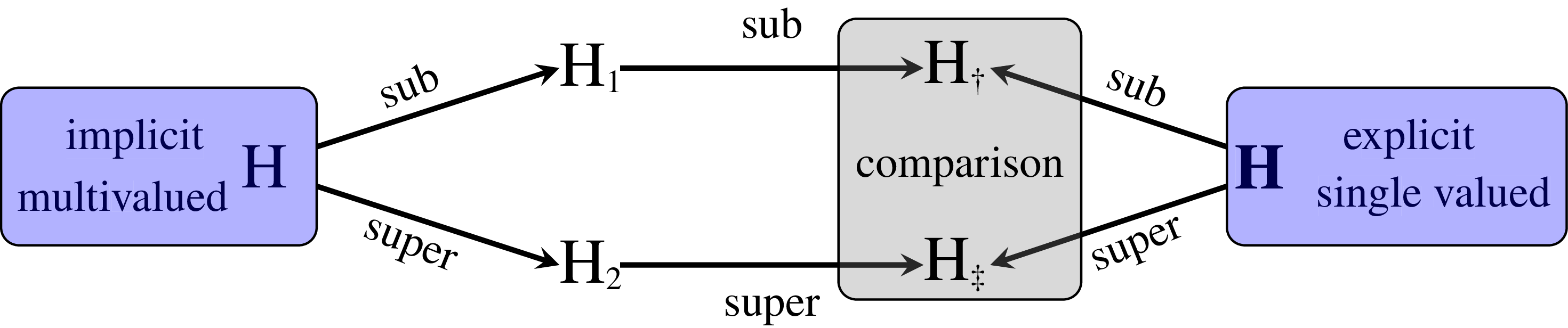
 f−λAf=h
 f−λBf=h
 H†
 H‡
 f−λH†f=h
 f−λH‡f=h
 H



