NOMENCLATURE
- C L, α
-
lift coefficient derivative with respect to pitching motion
- C L, q
-
lift coefficient derivative with respect to generic input
- f
-
dimensional frequency
- j
-
complex unit
 $\sqrt{-1}$
- l ref
-
reference length
- q
-
generic input signal
- M
-
cell volume matrix
- R
-
residual vector
- U ∞
-
freestream velocity
- w
-
vector of fluid unknowns
- x
-
vector of grid coordinates
- ω*
-
reduced frequency (
$\omega ^\ast =\frac{2\pi f\,l_{\text{ref}}}{U_{\infty} }$
) - |{}|
-
magnitude
- ∠{}
-
phase
-
$\hat{\lbrace \rbrace }$
-
Fourier coefficient
- {}0
-
steady state
- {}1
-
perturbation around steady state


1.0 INTRODUCTION
Certifying new airframes includes gust loads analysis and flutter clearance. Simulations have to be performed for a huge number of parameter combinations varying e.g. Mach number, altitude, load factor and gust length. Linear potential methods like doublet lattice(Reference Albano and Rodden1) cannot capture re-compression shocks and shock-induced separation. Thus, these methods cannot be applied at transonic flow conditions, where modern aircraft operate, without additional correction methods.(Reference Brink-Spalink and Bruns2,Reference Thormann and Dimitrov3) Solving the non-linear Reynolds-averaged Navier-Stokes (RANS) equations in a time-marching fashion coupled with a structural and flight dynamics solver, on the other hand, is prohibitive regarding the computational time required to cover the flight envelope.
In the industrial process, frequency response functions of integrated aerodynamic quantities are pre-computed instead and the fluid-structure problem is solved afterwards using e.g. a p-k method(Reference Rodden4) during the flutter analysis. A common approach applies sinusoidal structural excitations while integrating the RANS equations in time until the aerodynamic response becomes periodic. This process is repeated for each structural mode shape and several frequencies to interpolate the discrete output signal. If small disturbances are assumed, the aerodynamic system responds dynamically linear. The superposition principle can then be applied, leading to two computationally more efficient approaches.
In the first method, a non-periodic time-domain function – a pulse – is used to excite per mode a broad frequency range simultaneously.(Reference Seidel, Bennet and Whitlow5–Reference Thormann and Widhalm7) Since linearity is assumed, the aerodynamic response is a superposition of these excitation frequencies. Hence, the frequency response function can be obtained by a single time-domain simulation when dividing the Fourier transform of the output signal by the Fourier transform of the excitation signal. The second approach to reduce the computational cost, referred to as Linear (better linearised) Frequency-Domain (LFD) method, applies the small disturbance assumption to linearise the governing equations around a steady flow field. Thereafter, the equations are transferred into frequency domain resulting in a large, but sparse, linear system of equations for the perturbation of the fluid unknowns. The linear system is then solved at several frequencies to obtain the frequency responses per mode shape. The LFD method was first developed for turbo-machine applications(Reference Hall and Clark8,Reference Clark and Hall9) and later extended towards external aerodynamics. Published results comprise aerofoil cases,(Reference Dufour, Sicot, Puigt, Liauzun and Dugeai10,Reference Thormann, Nitsche and Widhalm11) isolated wings(Reference Pechloff and Laschka12,Reference Thormann and Widhalm13) and aircraft configurations.(Reference Thormann and Widhalm7,Reference Revalor, Daumas and Forestier14,Reference Widhalm, Thormann and Hübner15)
While the two approaches are well known, the aim of this paper is to analyse these methods at severe flow conditions close to the shock-buffet(Reference Lee16) onset. Hence, the application readiness of the methods is demonstrated at the edge of the flight envelope. Both methods rely on the superposition assumption and thus compute dynamically linear responses. Nevertheless, non-linear effects contained in the steady flow field like shock-induced separation are captured. Results of the LFD and pulse method are compared for a NACA 0010 aerofoil at a transonic Mach number and increasing angle-of-attack. In addition, frequency responses of lift and pitching moment as well as surface pressure coefficients are presented for a generic wing-fuselage configuration. The discussion is completed by detailed runtimes for the non-linear, time-marching approach and both time-linearised methods.
2.0 METHODS
2.1 Linearised frequency-domain solver
The LFD approach is first introduced. For a finite-volume method, the semi-discrete RANS equations can be written as
 $$\begin{eqnarray}
\frac{{\rm d}{M(x){{w}}}}{{\rm d}t} + {R}({w}, {x}, \dot{ {x}})&= 0,
\end{eqnarray}$$
with the diagonal matrix M storing the cell volumes and the residual function R depending on the vectors of fluid unknowns w, grid-point locations x and grid-point velocities
 $\dot{{{x}}}$
. Assuming small perturbations
 $({{w}}_1,{{x}}_1,\dot{{{x}}}_1)$
from a steady state (w
0, x
0), the variables can conveniently be separated as
 $$\begin{eqnarray*}
{{w}}(t) = {{w}}_0 + {{w}}_1(t), \qquad {{x}}(t) = {{x}}_0 + {{x}}_1(t), \qquad \dot{{{x}}}(t) = \dot{{{x}}}_1(t)\nonumber
\end{eqnarray*}$$
and Equation (1) can be linearised around this steady state
 $$\begin{eqnarray}
M \frac{{\rm d}{{{w}}_1}}{{\rm d}t} + {{R}}\left({{w}}_0, {{x}}_0\right) + \frac{{{{\partial R}}}}{{{{\partial w}}}} {{w}}_1 + \frac{{{{\partial R}}}}{{{{\partial x}}}} {{x}}_1 + \frac{{{{\partial R}}}}{\partial \dot{{{x}}}} \dot{{{x}}}_1 + {{w}}_0 \frac{\partial M}{{{\partial x}}} \dot{{{x}}}_1 = 0
\end{eqnarray}$$
The residual at steady state R(w 0, x 0) is assumed to be negligible small and Equation (2) is then transferred into the frequency domain
 $$\begin{eqnarray}
\left[\frac{{{{\partial R}}}}{{{{\partial w}}}} + j\omega ^\ast M\right]\widehat{{{w}}} = -\left[ \frac{{{{\partial R}}}}{{{{\partial x}}}} +j\omega ^\ast \left(\frac{{{{\partial R}}}}{\partial \dot{{{x}}}} + {{W}}_0 \frac{\partial M}{{{\partial x}}}\right)\right]{{\hat{x}}} ,
\end{eqnarray}$$
with j denoting the imaginary unit. The reduced frequency ω* has been normalised with the chord length and the free-stream velocity
 $$\begin{eqnarray}
\omega ^{\ast} = \frac{2\pi f\,l_{\text{ref}}}{U_{\infty}}
\end{eqnarray}$$
Equation (3) relates the Fourier coefficients of a harmonic excitation
 ${{\hat{x}}}$
to the Fourier coefficients of the fluid unknowns
 $\widehat{{{w}}}$
, constituting a large, but sparse, linear system of equations. In the frequency-domain approach, the flux Jacobian matrix is evaluated analytically, while the linearisation with respect to grid motion and velocity uses central finite differences. Including the linearisation of the turbulence model is crucial to accurately capture viscous effects like shock boundary-layer interactions. Further details concerning the LFD method in the DLR-TAU code and effects of simplifications within the Jacobian
 $\frac{{{{R}}}}{{{{w}}}}$
can be found in Ref. 13. The accuracy of this method depends on two assumptions: a dynamically linear response and a negligible steady-state residual. Especially the latter might be violated for complex geometries at challenging flow conditions. In a preliminary study, the mean solution of a time-accurate simulation was used in as linearisation point, when the steady solver did not converge, yielding still reasonable results.(Reference Thormann, Nitsche and Widhalm11)
The central part when applying an LFD method is solving the system of linear equations, corresponding to the exact order of the underlying spatial scheme, efficiently in terms of computational time and memory requirements. A generalised conjugate residual solver with deflated restarting is used, which recycles an invariant Krylov sub-space between restarts of the underlying generalised minimal residual solver.(Reference Xu, Timme and Badcock17) The linear system is pre-conditioned using an incomplete lower-upper factorisation of a blended flux Jacobian matrix resulting from first- and second-order spatial discretisations.(Reference McCracken, Ronch, Timme and Badcock18) Applying these methods significantly improved the robustness, providing convergence even at severe flow conditions.
2.2 Pulse excitation
A common approach to identify frequency response functions with a time-domain solver is to use a sinusoidal excitation while integrating in time until the response becomes periodic. This process is repeated for all frequencies of interest. However, if small disturbances are assumed, the aerodynamic system responds dynamically linear. The superposition principle can then be applied leading to a more efficient approach. A non-periodic time-domain function (e.g. a pulse, chirp or step) can be used to excite a broad frequency range. Hence, a frequency response function H per mode can be obtained from one single time-domain simulation when dividing the Fourier transform of the output signal by the Fourier transform of the excitation signal, e.g. for an arbitrary response ζ due to arbitrary input q,
 $$\begin{eqnarray}
H_{\zeta ,q}(\omega ^\ast ) = \frac{\mathcal {F}(\zeta (t)-\zeta _0)}{\mathcal {F}(q(t))},
\end{eqnarray}$$
with
 $\mathcal {F}$
denoting the Fourier operator. Since this approach assumes a linearly responding system, it belongs to the group of time-linearised methods, while avoiding an explicit linearisation of the underlying governing equations.
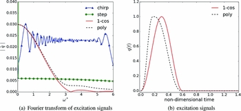
While the particular shape of the excitation function is not important, three criteria should be satisfied nevertheless. First, its Fourier transform should not exhibits roots in the magnitude at frequencies within the range of interest. An example is presented in Fig. 1(a) showing the Fourier transform of four excitation functions. While the chirp and the step functions result in a nearly constant magnitude over the relevant frequency range, the magnitude of the 1-cos function shows two roots and a significant decrease with increasing frequencies. Such behaviour can be avoided if a non-symmetric polynomial is used instead. The non-symmetric polynomial used in this study takes the specific form
 $$\begin{eqnarray*}
q(t) = (6t^2 -15t + 10)t^3 , \quad t \in [0,1]\nonumber
\end{eqnarray*}$$
for the ascending part of the pulse. The function is constructed with the boundary conditions, that the first and second derivative is zero at both endpoints of the interval. The final form is obtained by mirroring and stretching the polynomial for the descending part by a factor of three. Its time-domain representation as well as the 1-cos function are provided in Fig. 1(b). Both functions have the same compact support, while the polynomial exhibits its maximum earlier than the 1-cos function.
Fourier transforms of selected excitation signals and corresponding time histories of pulse excitations.

A compact support is the second criterion. Such support is preferred to reduce the number of grid deformation and preprocessing calls while integrating in time. Preprocessing is usually required to update the dual-grid metrics, but it is relatively fast compared with the deformation. For the wing-fuselage configuration discussed below, grid deformation and pre-processing combined account for almost as much computational time per physical time step as the iterations of the non-linear flow solver, which underlines the necessity to perform as few grid deformations as possible. Thus, using a chirp function as excitation, which offers almost ideal frequency content, would lead to significant computational overheads.
In the application of CFD solvers, smooth functions are preferable. While the chirp and the two pulse functions satisfy this condition, the step function does not. In the case of a step function, the grid velocity during the first time step is
 $$\begin{eqnarray}
\dot{x_1} \approx \frac{x_1(t+\Delta t) - x_1(t)}{\Delta t} = \frac{1}{\Delta t}
\end{eqnarray}$$
and hence inverse proportional to the time-step size. When severe flow conditions demand very small computational time steps, the grid velocity can become large, causing serious convergence issues for the time integrator. Therefore, applying a step function would constrain the minimum time-step size. Consequently, the non-symmetric polynomial pulse, satisfying all criteria, is used as excitation function throughout in this paper.
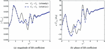
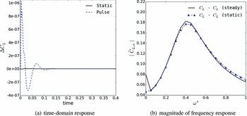
Applying the pulse technique comes with the assumption that a perturbation from the steady base state is caused by the excitation only. However, the initial steady computation is usually not converged to machine precision and additional fluctuations can occur, e.g. due to reflections from the far-field. These have an effect on the computed frequency response function especially if the excitation amplitude is small such as required at flow conditions exhibiting strong shock-induced separation. The calculation of response functions is improved by performing an additional time-dependent, static simulation. The perturbation of the output is computed by subtracting both signals instead of considering the difference to the steady solution only. Although the computational cost is nearly doubled, significant improvements can be observed at small and medium frequencies for the wing-fuselage case in pre-buffet, as shown in Fig. 2. While more detail for this configuration is discussed below, improved results are observed for reduced frequencies between 1 and 4 as well as for the quasi-steady part at zero reduced frequency.
Magnitude of lift frequency response for wing-fuselage configuration.

2.3 Computational fluid dynamics solver DLR-TAU
The DLR-TAU code(Reference Gerhold, Galle, Friedrich and Evans19,Reference Schwamborn, Gerhold and Heinrich20) is a finite-volume Euler and Navier-Stokes solver using hybrid grids. The chosen discretisation employs the modified scheme of Jameson, Schmidt and Turkel(Reference Jameson, Schmidt and Turkel21) for the mean-flow equations, while the Spalart-Allmaras(Reference Spalart and Allmaras22) one-equation turbulence model is used for the eddy-viscosity closure throughout in this paper. The flow equations are marched to steady state with a lower-upper, Symmetric-Gauss-Seidel pseudo-time integration method and geometric multi-grid. Time-accurate un-steady flow solutions can be obtained following the dual time-stepping approach(Reference Jameson23) combined with a second-order accurate backward differencing scheme.
3.0 RESULTS
3.1 NACA 0010
Results are presented for the NACA 0010 aerofoil using a computational domain discretised with about 30,000 points. The point distribution has a structured layer near the wall to ensure a sufficient boundary-layer resolution, while the far-field distance is set to 50 chord lengths. Results are shown at a constant Mach number of 0.8 and Reynolds number based on the chord length of 10million. Three angles of attack are analysed ranging from 3° to 5°.
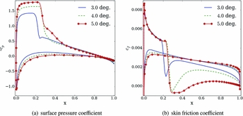
The steady surface pressure and skin friction coefficients are presented in Fig. 3. At an angle-of-attack of 3°, a re-compression shock can be observed at about 22% chord length while the flow remains attached. Increasing the angle-of-attack to 4° moves the shock downstream, while a small re-circulation region is observed. At an angle-of-attack of 5°, while the flow is still re-attaching before the trailing edge, the shock starts to move upstream, often referred to as inverse shock motion.
Steady surface pressure and skin friction coefficients for NACA 0010 aerofoil.

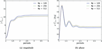
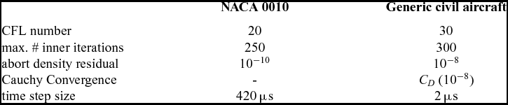
A rigid pitching motion is simulated around these different steady states with a rotational axis located at 25% chord length. A small amplitude of 10−5 degree is chosen to ensure a dynamically linear behaviour of the CFD solver. The dual-time stepping parameters are listed in the first column of Table 1. For all simulated angles of attack and time steps, the abort criterion based on the density residual was reached. A temporal convergence study is presented in Fig. 4 for a sinusoidal excitation at the highest angle-of-attack considered and reduced frequency of 0.4. The complex-valued derivative of the lift coefficient is computed using a sliding window to understand when the lift derivative converges. Convergence is achieved after about 2.5periods. Increasing the number of time steps per period (Np) from 128 to 256 reduces the lift coefficient’s magnitude and increases its phase. A further refinement of the time-step size has a negligibly small effect on the results.
Temporal convergence of lift coefficient for NACA 0010 at 5° angle-of-attack and a reduced frequency of 0.4.

Dual-time stepping parameters

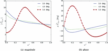
Before comparing results computed with the different methods, a more general discussion of the lift coefficient’s frequency response is given in Fig. 5. A reduced frequency resolution of 0.05 is chosen to provide a smooth frequency response function. This corresponds to 0.535s simulated physical time when using the pulse method. At an angle-of-attack of 3°, the frequency response is qualitatively comparable with Theodorsen’s aerodynamics.(Reference Theodorsen24) A monotonic decrease in magnitude and a phase lag at small reduced frequencies is observed. The small region of separation at 4° angle-of-attack is reducing the quasi-steady derivative, while the magnitude is still decreasing monotonically over the reduced frequency range. The shape of the frequency response function is different for the highest angle-of-attack, caused by the stronger interaction between the shock and the region of separated flow. Since the quasi-steady derivative is further reduced, this test case is in the non-linear region of the C L − α polar. Moreover, the magnitude is now exhibiting a maximum around a reduced frequency of about 0.4, and for reduced frequencies below the maximum, a phase lead is observed. This behaviour was linked to a weakly damped eigenvalue of the fluid Jacobian matrix. Such resonance behaviour was previously analysed in the context of shock buffet in Refs 25 and 26 and discussed for validation of the LFD method in Ref. 11.
Frequency responses in lift coefficient for NACA 0010 aerofoil.

The time-domain lift response due to the pulse excitation as well as for the static simulation is shown in Fig. 6(a) for the 5° angle-of-attack case. Although fluctuations obtained from the static simulation are two orders of magnitude smaller than the response due to the pulse, an influence on the frequency response function is observed in Fig. 6(b). The quasi-steady derivative is improved – indicating a small drift of the mean solution – as well as the magnitude at higher frequencies.
Time-domain lift response of pulse and static computation and comparison of frequency response function for NACA 0010 aerofoil at incidence of 5°.

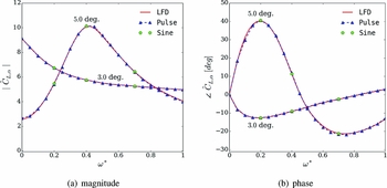
A comparison of the frequency response functions computed with both the LFD and time-domain methods using either sinusoidal or pulse excitation is given in Fig. 7 for the attached-flow case at 3° angle-of-attack and the most severe case at 5°. An excellent agreement is obtained between the LFD and the pulse method for the complete frequency range considered, even at the severe pre-buffet flow condition. Computations using sinusoidal excitations were performed at three reduced frequencies, confirming the validity of the time-linearised approaches for attached as well as detached steady flow conditions. Computational performance is not discussed for this academic test case. This will be done for the aircraft configuration instead.
Comparison of frequency responses in lift coefficient for NACA 0010 aerofoil.

3.2 Generic civil aircraft
The second test case is a half wing-body configuration scaled to wind-tunnel dimensions. The semi-span of the model is 1.10m and the aerodynamic mean chord is about 0.279m. The wing is twisted, tapered and has a constant sweep angle of 25°. This configuration has recently been investigated in the transonic wind-tunnel facility of the Aircraft Research Association,(Reference Lawson, Greenwell and Quinn27) and it was also chosen for investigation of global stability analysis.(Reference Timme and Thormann28)
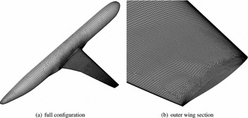
An un-structured mesh was produced using the Solar grid generator.(Reference Martineau, Stokes, Munday, Jackson, Gribben and Verhoeven29) The initial spacing normal to all viscous walls is less than 0.8 in wall units for this coarse mesh, while the growth rate of cell sizes in the viscous layer is less than 1.3. The blunt trailing edge is described by 8 cells corresponding to a spacing of about 0.15% of the local chord. Concerning the span-wise mesh distribution, a spacing of 0.5% and 0.1% of the span is imposed for the wing root and tip, respectively. Altogether, the grid is composed of 2.7million points corresponding to 4.7million elements of mixed type including 12,000 prisms, 71,000 pyramids, 2.4million hexahedral and 2.3million tetrahedral elements. The grid spacing on the wing surface is presented in Fig. 8.
Generic wing-fuselage configuration.

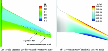
The freestream Mach number is set to 0.8 and the Reynolds number based on the aerodynamic mean chord is 3.75million. Fully turbulent flow is assumed. The angle-of-attack in the current study is fixed at 3°, just below shock-buffet onset. The reference temperature and pressure are 266.5K and 66.0kPa, respectively. Far-field conditions are applied at a distance corresponding to 25 times the semi-span of the model (around 90 aerodynamic mean chords), while symmetry boundary condition is applied along the centre plane. The steady surface pressure distribution on the wing is depicted in Fig. 9(a) showing a shock at about 50% chord length. The shock-induced separation – marked by a black, dashed line – starts at mid-semi-span with reattachment further downstream, whereas in the outer wing section, between 79% and 91% of the semi-wing span, the flow is detached all the way from the re-compression shock to the trailing edge. Around this steady flow field, forced-motion simulations are performed exciting the system in a synthetic torsion mode, as shown in Fig. 9(b). The parameter settings for the dual-time stepping are listed in the second column of Table 1.
Steady surface pressure and z-component of excitation mode.

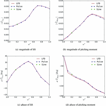
The frequency response in lift and moment coefficient computed with the LFD and pulse method is presented in Fig. 10. A reduced frequency range between 0.0 and 1.0 based on the mean aerodynamic chord is considered. The reduced frequency resolution of the pulse method is 0.1, which corresponds to a simulated physical time of 0.3s. The magnitude of the lift exhibits a local maximum around reduced frequency 0.7 (see Fig. 10(a)). A similar behaviour can be observed for the pitching moment in Fig. 10(b). This is contrary to linear potential theory, where starting from the quasi-steady derivative a monotonic decrease is predicted for torsion-dominated modes. Analysing the phase of the lift coefficient, a maximum and an inflection point can be observed as well as a phase lead over a wide range of reduced frequencies. A similar behaviour has been observed for the aerofoil case in Fig. 7. The results computed by both time-linearised methods agree excellently in the considered frequency range for the lift and moment despite this complex response behaviour. A solution using the time-domain method with sinusoidal excitation is shown for reduced frequency 0.2, confirming the time-linearised results.
Comparison of frequency responses for generic civil aircraft.

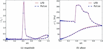
Figure 11 presents unsteady pressure coefficients at 90% semi-span; a position where the steady flow field exhibits separation as shown in Fig. 9(a). The magnitude is dominated by a strong peak at about 40% of the local chord length, showing the movement of the re-compression shock. Upsteam of the shock, in the supersonic region, only minor pressure fluctuations can be seen, while the separation bubble causes pressure fluctuations near the trailing edge. A discontinuity of about 145° can be observed in phase at the same chord-wise position as the shock peak. A monotonic increase in phase from leading to trailing edge is seen on the lower surface with subsonic flow. All these features are captured well by the LFD and the pulse method at this pre-buffet flow condition showing the maturity of both time-linearised approaches for three-dimensional geometries.
Comparison of complex-valued surface pressures at reduced frequency of 0.5 for wing-body configuration at normalised span position of 0.9.

Finally, the runtimes of the different methods are compared for the generic wing-fuselage configuration in Table 2. Both LFD and the non-linear, time-domain method using sinusoidal excitation evaluate one frequency at a time, whereas the former approach is 150 times faster in comparison. A reduction in computational time of more than an order of magnitude compared to the sinusoidal time-domain simulations is still achieved when the pulse method is applied. The pulse method is slower than the LFD, since an additional static simulation was required and higher frequencies are evaluated as well, which are not of interest in an aeroelastic application. A larger time-step size than than the used 2μs would directly improve the speed-up of the pulse method and reduce the number of unnecessarily computed frequency responses. However, a previous time-convergence analysis(Reference Sartor and Timme30) in the context of shock buffet has shown that larger time steps have a negative influence on the prediction quality at these severe flow conditions. At more benign flow conditions, the convergence requirements of the non-linear, time-dependent solver are less stringent, and hence the cost-savings of LFD become less dominant. Experience has shown that a cost-saving factor of about five between LFD and pulse is often observed in attached transonic flow. Overall, an order of magnitude speed-up between each of the presented simulation approaches to calculate aerodynamic derivatives is a fair estimate. Moreover, while LFD only requires a monitoring of the aerodynamic derivatives to judge the convergence of the linear system, time-dependent simulations require expensive investigation of temporal convergence, such as real time-step size and number of sub-iterations/abort criteria. In addition, an appropriate excitation amplitude has to be chosen. This cost is not included in the table.
Runtimes for generic civil aircraft using 72 cores of Intel E5-2660 with 2.2GHz

4.0 CONCLUSION
Two approaches are presented to reduce the computational cost of calculating frequency response functions of aerodynamic derivatives for aeroelastic applications. Both methods rely on the assumption of a dynamically linear responding system. The first approach linearises the flow equations and solves the resulting system in the frequency domain. A robust iterative technique based on a Krylov sub-space method is applied to efficiently solve the large but sparse linear system. The second method uses pulse excitation in the time domain to compute the entire frequency response function within one simulation. A non-symmetric, polynomial function with compact support (i.e., a pulse) is used to excite a broad frequency spectrum while minimising the amount of grid deformation calls. Results are presented for the NACA0010 aerofoil as well as for a generic wing-fuselage configuration. Excellent agreement between both time-linearised methods and the time-marching simulations using sinusoidal excitation are obtained for both test cases comparing frequency response functions of lift and moment coefficients as well as local pressure distributions. Even at edge-of-envelope flow conditions including shock-induced separation close to the buffet onset, time-saving factors of 1 order of magnitude are achieved comparing the pulse method to non-linear, time-domain simulations using sinusoidal excitation. Applying the linearised frequency domain method provides an additional order of magnitude in speed-up to enable routine computational aeroelasticity.
Comparing both time-linearised approaches, the frequency domain method is faster if responses in a limited frequency range are of interest and a non-uniform sample distribution is desired. In addition, no expensive time-convergence or amplitude analyses are required. If responses are desired for a large frequency range, the pulse method is computationally more efficient. Moreover, it is a reasonable alternative if a Jacobian matrix or the matrix-free product of the Jacobian and a vector is not implemented for the chosen type of flux discretisation or turbulence model.