1. Introduction
It is well known that a proper increase in shear rate or plume coherency can both enhance heat transport in turbulent Rayleigh–Bénard convection (RBC). An interesting question is which of the two effects, plume or shear, is more important for the transport properties. RBC is a paradigmatic system for studying turbulent transport, it considers a fluid layer heated from below and cooled from above. In RBC, heat is transferred spontaneously from the bottom to the top. When the thermal drive is strong enough, two thermal boundary layers are developed adjacent to the top and bottom plates which account for most of the temperature drop, meanwhile the bulk region is well mixed. During the past decades, RBC has attracted numerous experimental, theoretical and numerically studies (Ahlers, Grossmann & Lohse Reference Ahlers, Grossmann and Lohse2009; Lohse & Xia Reference Lohse and Xia2010; Chillà & Schumacher Reference Chillà and Schumacher2012; Xia Reference Xia2013). The system is controlled by the Rayleigh number  $Ra = \alpha g{\rm \Delta} H^3/(\nu \kappa )$ and the Prandtl number
 $Pr = \nu /\kappa$, which describe the non-dimensional thermal driven strength and the property of working fluid, respectively. Here,
 $\alpha$ is the thermal expansion coefficient,
 $g$ is the acceleration due to gravity,
 $\varDelta$ is the temperature difference between the top and bottom plates,
 $H$ is the height of the convection domain,
 $\nu$ is the kinematic viscosity and
 $\kappa$ is the thermal diffusivity. On the other hand, the system has two response parameters, namely, the Nusselt number
 $Nu = Q/k(\varDelta /H)$, which describes the non-dimensional heat transfer efficiency, and the Reynolds number
 $Re = UH/\nu$. Here,
 $Q$ is the total (vertical) heat flux,
 $k$ is the thermal conductivity of the working fluid and
 $U$ is a typical velocity of the flow. A central issue in study RBC is to determine
 $Nu(Ra,Pr)$ and
 $Re(Ra,Pr)$. It is generally believed that, in the so-called classical regime, heat transfer in RBC is controlled by the boundary layers (BLs). For moderate Rayleigh number, a large-scale circulation (LSC) exists in RBC (Krishnamurti & Howard Reference Krishnamurti and Howard1981; Cioni, Ciliberto & Sommeria Reference Cioni, Ciliberto and Sommeria1997; Qiu & Tong Reference Qiu and Tong2001; Xia, Sun & Zhou Reference Xia, Sun and Zhou2003; Funfschilling & Ahlers Reference Funfschilling and Ahlers2004; Xi, Lam & Xia Reference Xi, Lam and Xia2004; Xi & Xia Reference Xi and Xia2007). The LSC sweeps over the conducting plate with a mean wind velocity
 $U$, thus directly shearing the BL therein. The velocity BL thickness
 $\delta _U$ and thermal BL thickness
 $\delta _T$ can be determined by the Prandtl–Blasius BL theory (Landau & Lifshitz Reference Landau and Lifshitz1987),
 $\delta _u, \delta _T \sim Re^{1/2}$. In fact, these classical relations also serve as the key assumptions of the Grossmann–Lohse theory (Grossmann & Lohse Reference Grossmann and Lohse2000, Reference Grossmann and Lohse2001, Reference Grossmann and Lohse2002, Reference Grossmann and Lohse2004), which has achieved great success in predicting the complex
 $Nu(Ra,Pr)$ and
 $Re(Ra,Pr)$ behaviours. Besides, if the Rayleigh number is large enough, it is believed that the BL will eventually become turbulent, which is also known as the ‘ultimate’ regime (Kraichnan Reference Kraichnan1962). Transition to the ultimate regime is expected when the shear Reynolds number exceeds a critical value
 $Re_s = \delta _uU/\nu = a\sqrt {Re} \ge 420$, where
 $a$ is a constant of order unity (Landau & Lifshitz Reference Landau and Lifshitz1987). When the system is in the ultimate regime, the Nusselt number is expected to follow the ultimate scaling
 $Nu \sim Ra^{1/2}$, with a possible logarithmic correction (Chavanne et al. Reference Chavanne, Chillà, Castaing, Hébral, Chabaud and Chaussy1997; Roche et al. Reference Roche, Gauthier, Kaiser and Salort2010; Grossmann & Lohse Reference Grossmann and Lohse2011; He et al. Reference He, Funfschilling, Nobach, Bodenschatz and Ahlers2012).
Although the strength of the wind and the associated shear are important in determining the heat transfer efficiency, it is notoriously difficult to push up the Rayleigh number and thus the shear Reynolds number to attain the ultimate regime. A potentially promising way is to directly impose a shear stress at the boundary. This is sometimes called sheared RBC or turbulent mixed convection. The early experimental work of Ingersoll (Reference Ingersoll1966) used a rotating annulus lid to generate an external shear, and the author reported a subtle reduction in heat transfer. Solomon & Gollub (Reference Solomon and Gollub1990) used a magnetically stirred thin layer of mercury to shear the bottom of a water layer, and they observed a slight increase in Nusselt number. Recently, Shevkar et al. (Reference Shevkar, Gunasegarane, Mohanan and Puthenveettil2019) used an external blower to directly shear the thermal BL, and found that shear can align the line plumes and increase their mean spacing.
Direct numerical simulation (DNS) has also been widely used to study the effect of external shear on RBC. Scagliarini, Gylfason & Toschi (Reference Scagliarini, Gylfason and Toschi2014) applied a horizontal pressure gradient to shear the boundary in RBC. They found that the vertical heat flux first decreases due to the sweeping of plumes, and then increases when the shear dominates over buoyancy. Similar behaviour of heat transfer has also been observed for mixed convection in a long channel (Pirozzoli et al. Reference Pirozzoli, Bernardini, Verzicco and Orlandi2017) and a cylindrical RBC cell with a rotating lid (Vishnu & Sameen Reference Vishnu and Sameen2020). Blass et al. (Reference Blass, Zhu, Verzicco, Lohse and Stevens2020) introduced wall shear by combining the plane Couette flow with RBC, and they identified three different regimes using the Monin–Obukhov length scale. When the flow is dominated by shear, the convection domain is filled with large-scale meandering rolls and the Nusselt number  $Nu$ shows an approximate
 $Ra^{1/3}$ scaling. In a subsequent study (Blass et al. Reference Blass, Tabak, Verzicco, Stevens and Lohse2021), the Prandtl number effect of sheared RBC is also explored. It is also worth mentioning that the intricate interplay between buoyancy and shear is also an important issue in studying the atmospheric BL (Deardorff Reference Deardorff1972; Garratt Reference Garratt1994; Samir & James Reference Samir and James1998).
Despite the fact that the BL to a large extent determines the heat flux of RBC, the heat transfer in the bulk region is, however, accomplished by another turbulent coherent structure, namely the thermal plume. Plumes can also be viewed as the detached BLs (Grossmann & Lohse Reference Grossmann and Lohse2004). More importantly, they are the elementary heat carriers and are responsible for most of the vertical heat transport in the system (Shang et al. Reference Shang, Qiu, Tong and Xia2003; Shang, Tong & Xia Reference Shang, Tong and Xia2008; Zhou & Xia Reference Zhou and Xia2010). Inspired by these facts, the pioneering work of Huang et al. (Reference Huang, Kaczorowski, Ni and Xia2013) reported, for the first time, that with proper geometrical confinement, the heat transfer in RBC can be controlled by the plumes, instead of the boundary layer. The plume-controlled regime is featured by an increase in plume coherency and the condensation of coherent structures (Chong et al. Reference Chong, Huang, Kaczorowski and Xia2015). In addition to lateral confined RBC, the concept of coherent structure manipulation can also be generalized to other dynamical systems (Chong et al. Reference Chong, Yang, Huang, Zhong, Stevens, Verzicco, Lohse and Xia2017; Lim et al. Reference Lim, Chong, Ding and Xia2019).
As mentioned above, heat transfer enhancement in turbulent RBC can be achieved by increasing either shear or plume coherency. In a recent study, Zhang, Ding & Xia (Reference Zhang, Ding and Xia2021) conducted an experimental and numerical study on turbulent RBC in the presence of an effective horizontal buoyancy (experimentally generated by cell tilting) and found that these two effects can indeed coexist. They introduced a modified free fall time scale  $\tau = \sqrt {H/(\cos \beta \alpha {\rm \Delta} g)}$ to normalize the governing equations and obtain
 \begin{gather} \frac{\partial \boldsymbol{{u}}^\prime}{\partial t^\prime} + \textbf{{u}}^\prime\boldsymbol{\cdot}\boldsymbol{\nabla}\boldsymbol{{u}}^\prime ={-}\boldsymbol{\nabla} p^\prime + \sqrt{\frac{Pr}{Ra_V}}\nabla^2\boldsymbol{{u}}^\prime + T^\prime\hat{\boldsymbol{{z}}} + \frac{Ra_H}{Ra_V}T^\prime\hat{\boldsymbol{{x}}}, \end{gather}
 \begin{gather}\frac{\partial T^\prime}{\partial t^\prime} + \boldsymbol{{u}}^\prime\boldsymbol{\cdot}\boldsymbol{\nabla} T^\prime = \sqrt{\frac{1}{Ra_V Pr}}\nabla^2T^\prime, \end{gather}
 \begin{gather}\boldsymbol{\nabla}\boldsymbol{\cdot} \boldsymbol{{u}}^\prime = 0, \end{gather}
where,  $Ra_H = \alpha g \sin {\beta }{\rm \Delta} H^3/(\nu \kappa )$ and
 $Ra_V = \alpha g \cos {\beta }{\rm \Delta} H^3/(\nu \kappa )$ are the horizontal Rayleigh number and the vertical Rayleigh number, respectively. Their ratio
 $\varLambda = Ra_H/Ra_V$ is defined as the buoyancy ratio. Moreover, they generalized the Nusselt number to a vector Nu, whose vertical and horizontal components are
 $Nu_V$ and
 $Nu_H$, respectively. Unlike most previous studies on tilted RBC, in which
 $Ra_H$ and
 $Ra_V$ are both varying with the tilting angle
 $\beta$, Zhang et al. (Reference Zhang, Ding and Xia2021) fixed the vertical Rayleigh number
 $Ra_V$ in their experiment by simultaneously tilting the cell by an angle
 $\beta$ and raising the temperature difference across the conducting plates
 $\varDelta$ by a factor of
 $1/\cos {\beta }$ accordingly. They found that the vertical heat transport efficiency (
 $Nu_V$) in the system increased monotonically with the buoyancy ratio
 $\varLambda$. However, in such a case, increases of shear and plume coherency occur concurrently with the increasing effective horizontal buoyancy. A very interesting question is that which effect, plume or shear, dominates the observed enhancement in
 $Nu_V$ and which mechanism is more efficient in promoting heat transfer.
To address the above question, in this study, we carry out an experimental and numerical investigation that is designed to explore the effects of plume and shear. This is achieved by varying the aspect ratios of a rectangular convection cell and tilting it at the same time. We use water as the working fluid and the Prandtl number is kept at  $Pr = 4.3$ throughout this work. For small Prandtl number working fluids (gases or liquid metals), the system may behave quite differently due to its relatively large thermal diffusivity (Zwirner & Shishkina Reference Zwirner and Shishkina2018; Zürner et al. Reference Zürner, Schindler, Vogt, Eckert and Schumacher2019; Zwirner et al. Reference Zwirner, Khalilov, Kolesnichenko, Mamykin, Mandrykin, Pavlinov, Shestakov, Teimurazov, Frick and Shishkina2020). Combining experiments with DNS, we apply streamwise and spanwise confinements to turbulent thermal convection in the presence of an effective horizontal buoyancy using the platform of tilted RBC reported in Zhang et al. (Reference Zhang, Ding and Xia2021). The rest of the paper is organized as follows: the details of the experimental set-up and the procedures of particle image velocimetry and thermochromic-liquid-crystal measurements are described in § 2. A brief introduction to the numerical method is provided in § 3. We then present the main results in § 4. In § 5, we will analyse the energetics of the problem at hand and put forward the generalized expressions for various energy pathways and the mixing efficiency of the system. Finally, we summarize the present work in § 6.
2. Experimental set-up
2.1. The convection cell
In the experiment, we use a rectangular convection cell whose height, length, width are  $H = 126$ mm,
 $L = 126$ mm,
 $W = 38$ mm, respectively (Huang & Xia Reference Huang and Xia2016). The coordinate system is set in the frame of the convection cell with the
 $z$-axis pointing from the bottom plate to the top plate, and gravity lies in the
 $x$–
 $z$ plane. In such a case, the LSC is developed robustly in the
 $x$–
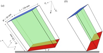
 $z$ plane (Shishkina & Horn Reference Shishkina and Horn2016; Zhang et al. Reference Zhang, Ding and Xia2021). In the present study, tiling is applied in two ways: when it is applied along the length of the cell (see figure 1a), the aspect ratios of the cell are
 $\varGamma _x = L/H = 1, \varGamma _y = W/H = 0.3$. In such a configuration, confinement is applied in the spanwise direction and hereafter we refer to this as spanwise confinement; the corresponding scenario with
 $\varGamma _x = 0.3, \varGamma _y = 1$ is referred to as streamwise confinement (see figure 1b). Both the top and bottom plates are made of copper (
 $k_{Cu} = 386\ {\rm W}\ {\rm m}^{-1}\ {\rm K}^{-1}$), and the sidewall is made of Plexiglas which is 4 mm in thickness. The top plate is cooled by a refrigerator (PolyScience) and the bottom plate is heated by a resistive heater. We embed three thermistors (OMEGA Engineering, Model 44031) in each plate to monitor the temperature therein. The temperature signals are acquired using a multi-channel digital multimeter (Keysight, Model 36972A). We use distilled and deionized water as the convecting fluid and the bulk temperature is set to be 40
 $^\circ$C, corresponding to a Prandtl number of
 $Pr = 4.3$. We also use a cooper basin to compensate for heat leakage from the bottom plate and wrap plastic foam (approximately 5 cm in thickness) around the cell to prevent heat leakage from the sidewall. Finally, the cell is anchored on a stage which is able to rotate. The convection cell and the stage are placed in a home-made thermostat whose temperature is set equal to the bulk temperature of the fluid. The temperature stability of the thermostat is about
 $\pm$0.02 K.
Schematics of the convection cells with (a) spanwise confinement ( $\varGamma _x = 1, \varGamma _y = 0.3$) and (b) streamwise confinement (
 $\varGamma _x = 0.3, \varGamma _y = 1$). The effective horizontal buoyancy is applied in the
 $x$-direction. The green sheets denote the planes in which velocity (PIV) and temperature thermochromatic liquid-crystal measurements are made.

2.2. Particle image velocimetry
To quantify the flow fields, we conduct particle image velocimetry (PIV) measurements. A continuous laser sheet (CNI, 532 nm in wavelength) is used for illumination. The laser sheet illuminates the centre  $x$–
 $z$ plane of the cell. The tracing particles are 20
 $\mathrm {\mu }$m in diameter (Dantec, PSP polyamide particles). We use a CCD camera (IDS UI-3370C,
 $2048 \times 2048$ pixels in resolution), working in monochrome mode, to capture the image sequences. The frame rate of the camera is 10 Hz. Image post-processing and velocity field calculations are processed using a commercial software package (LaVision, DaVis 10). Over 10 000 velocity maps are calculated for each run to ensure statistical convergence.
2.3. Liquid-crystal measurement
The thermochromic-liquid-crystal (TLC) technique (Zhou, Sun & Xia Reference Zhou, Sun and Xia2007; Zhou & Xia Reference Zhou and Xia2010) is used to visualize the temperature field. The colour of TLC depends on the temperature of the working fluid. In this work, we use TLC micro-spheres (Hallcrest, R40C5W) to indicate the local temperature in the flow. The TLC particles are suspended in the working fluid with a concentration of approximately 0.01 % by weight, thus their influence on the fluid and the flow can both be neglected. A white light sheet, generated by a xenon lamp (SOFN, 7ILX500) projecting onto a slit, is used for illumination. The position of the illumination plane is the same as that of PIV measurement, and the thickness of the white light sheet is approximately 2 mm. We use the same camera as the PIV measurements (IDS UI-3370C), but now working in RGB (red, green, blue) colour mode, to capture the TLC images. The light scattered by the TLC micro-spheres changes from red to green, then to blue as the temperature is increased from 40 to 45  $^\circ$C. Outside this temperature window, the suspension is clear. Since the temperature window of the TLC is centred around 42.5
 $^\circ$C, the bulk temperature is also set to be 42.5
 $^\circ$C for the liquid-crystal measurement, corresponding to a Prandtl number of
 $Pr = 4.2$. The slight change in Prandtl number is known to have a negligible effect on the flow (Lam et al. Reference Lam, Shang, Zhou and Xia2002; Xia, Lam & Zhou Reference Xia, Lam and Zhou2002).
3. Direct numerical simulation
As a complement to the experiments, we also conduct DNS to obtain more quantitative information of both the velocity and temperature fields. We use the  $ {CUPS}$ code, which solves the governing equations using a fourth-order finite-volume method on staggered velocity and temperature grids. A multi-resolution scheme is also adopted to promote the efficiency of solving the momentum equation. For a detailed description of the code, the reader is referred to Chong, Ding & Xia (Reference Chong, Ding and Xia2018). All boundaries are no slip and impermeable. The temperature at the top and bottom plates are set to be
 $-$0.5 and 0.5, respectively. The sidewalls are adiabatic. Both the temperature and velocity grids fulfil the resolution requirement proposed by Shishkina et al. (Reference Shishkina, Stevens, Grossmann and Lohse2010).
4. Results
4.1. Heat transfer
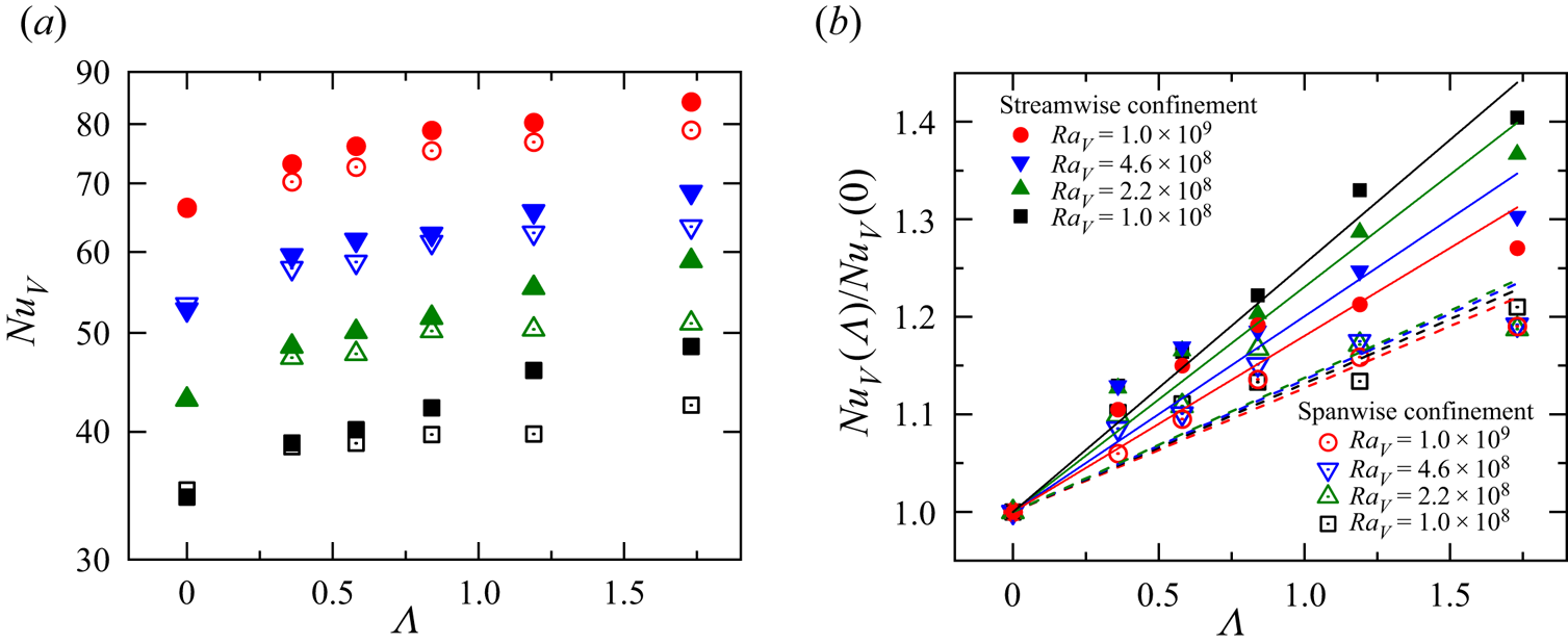
We first plot in figure 2(a) the experimentally measured vertical Nusselt number  $Nu_V$ as a function of the buoyancy ratio
 $\varLambda$ for cells with streamwise confinement (
 $\varGamma _x = 0.3, \varGamma _y = 1$) and spanwise confinement (
 $\varGamma _x = 1, \varGamma _y = 0.3$), respectively. Figure 2(b) shows the corresponding normalized vertical Nusselt numbers
 $Nu_V(\varLambda )/Nu_V(0)$. The legends in figures 2(a) and 2(b) are the same. The vertical Rayleigh number ranges from
 $Ra_V = 10^8$ to
 $10^9$ and the maximum buoyancy ratio is
 $\varLambda = 1.73$, corresponding to a tiling angle of
 $\beta = 60^\circ$. For small values of the buoyancy ratio, the vertical heat transfer efficiencies in streamwise and spanwise confinement cells are close to each other. As we increase the buoyancy ratio, the
 $Nu_V-\varLambda$ curve for a streamwise confined cell shows a more rapid increase than the spanwise confined one. The difference in
 $Nu_V$ is most apparent at small
 $Ra_V$ and large
 $\varLambda$. Figure 2(b) shows a clearer view of the relative increase in
 $Nu_V$. It is seen that the normalized vertical Nusselt numbers of the spanwise confined case (open symbols) basically collapse onto a single curve. The slopes of linear trend with
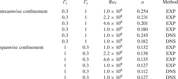
 $Nu_V(\varLambda )/Nu(0) = 1 + a\varLambda$ (the dashed lines in figure 2b) range from 0.127 to 0.138, which is close to the value of 0.14 for a cylindrical cell with unity aspect ratio (Zhang et al. Reference Zhang, Ding and Xia2021). On the other hand, the increase in
 $Nu_V$ is considerably higher for the streamwise confined cell, and its rate of increase strongly depends on the vertical Rayleigh number, i.e. the curve with small
 $Ra_V$ shows a faster increase in
 $Nu_V$. For the lowest vertical Rayleigh number
 $Ra_V = 10^8$, the slope of a linear fitting gives 0.254, corresponding to an enhancement approximately 40 % at
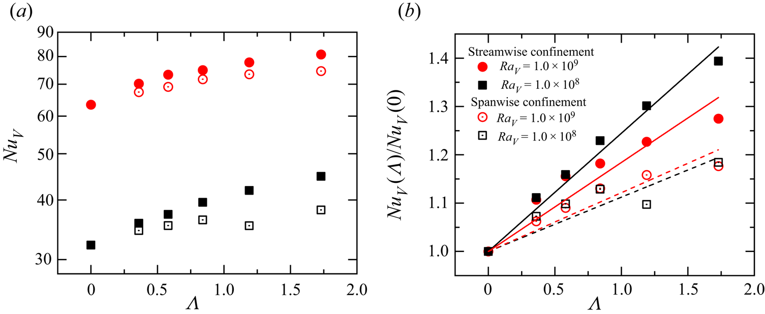
 $\varLambda = 1.73$. Figures 3(a) and 3(b) show
 $Nu_V$ and
 $Nu_V(\varLambda )/Nu_V(0)$ obtained by DNS, respectively. The numerical results in general agree well with our experimental findings. The linear fitting parameters of both the experimental and numerical data are summarized in table 1. Although the linear fitting is only a first-order approximation, the analysis above reveals the important fact that, in turbulent RBC with an effective horizontal buoyancy, applying streamwise confinement is more efficient in promoting the vertical heat transport than applying spanwise confinement. We also note that, for large values of buoyancy ratio
 $\varLambda$, the data points in figures 2(b) and 3(b) show some deviation from the linear fittings, for which we do not yet have any explanation. At this stage, a systematic exploration or a theoretical treatment of such high-order effects of the
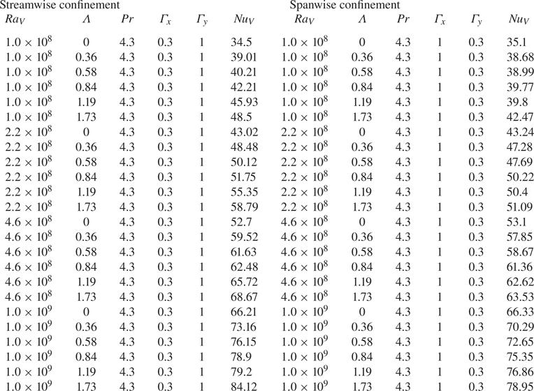
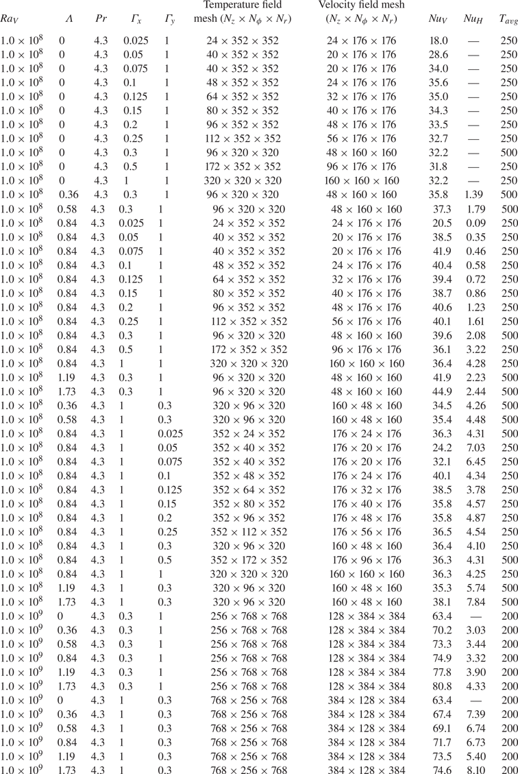
 $Nu_V-\varLambda$ relation is beyond the scope of this study. The full experimental and numerical data sets are listed in the Appendix.
(a) Experimentally measured vertical Nusselt number  $Nu_V$ as a function of the buoyancy ratio
 $\varLambda$ for different vertical Rayleigh numbers
 $Ra_V$. Solid symbols correspond to cell with streamwise confinement (
 $\varGamma _x = 0.3, \varGamma _y = 1$), open symbols denote cell to spanwise confinement (
 $\varGamma _x = 1, \varGamma _y = 0.3$); (b) the corresponding normalized vertical Nusselt number as a function of the buoyancy ratio for different
 $Ra_V$. The solid and dashed lines show first-order linear fittings to the data.

DNS results. (a) Vertical Nusselt number  $Nu_V$ as a function of the buoyancy ratio
 $\varLambda$. Solid symbols correspond to streamwise confinement (
 $\varGamma _x = 0.3, \varGamma _y = 1$), open symbols denote spanwise confinement (
 $\varGamma _x = 1, \varGamma _y = 0.3$); (b) the corresponding normalized vertical Nusselt number. The solid and dashed lines show linear fittings to the data.

Fitting parameters of  $Nu_V(\varLambda )/Nu_V(0) = 1 + a\varLambda$.

4.2. Flow dynamics
For thermal convection systems, the change in the heat transfer property is usually accompanied by a change in the flow morphology. In this subsection, we will discuss the properties of both the temperature and velocity fields as well as the statistical properties of various profiles measured at the mid-height of the cells with different confinement settings.
4.2.1. The temperature and velocity fields
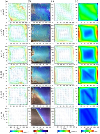
We show in columns (a) and (b) of figure 4 the experimentally measured instantaneous velocity fields (by PIV measurement) and temperature fields (by liquid-crystal measurement) in the centre  $x$–
 $z$ plane of a spanwise confined cell (
 $\varGamma _x = 1, \varGamma _y = 0.3$), respectively. The vertical Rayleigh number is fixed at
 $Ra_V = 10^9$. In practice, the cell for the nominally levelled case is tilted deliberately by one degree (
 $\varLambda = 0.02$) to lock the LSC (Funfschilling & Ahlers Reference Funfschilling and Ahlers2004; Brown & Ahlers Reference Brown and Ahlers2006; Xi, Zhou & Xia Reference Xi, Zhou and Xia2006; Xi & Xia Reference Xi and Xia2008). Meanwhile, the velocity fields are coarse grained for a clearer view of the reader. The change in flow morphology is similar to those found in cylindrical cells (Zhang et al. Reference Zhang, Ding and Xia2021): with increasing buoyancy ratio, the LSC undergoes an elliptic-to-square change; the mean flow expands towards the peripheral of the cell, and leaves a ‘stagnant’ region in the bulk. Such behavioural change is more evident in the temperature field (see figure 4b). For the levelled case, the hot (blue region) and cold (red region) plumes can travel through the bulk region intermittently. While for moderate buoyancy ratios (
 $0.36\le \varLambda \le 1.19$), the down-welling cold plumes and the up-welling hot plumes are vigorous but constrained near the sidewalls of the cell. Meanwhile, a stably stratified temperature gradient is gradually established in the bulk. For the highest buoyancy ratio
 $\varLambda = 1.73$, the flow is nearly steady, thermal plumes only survive in the corners of the cell and can hardly penetrate through the bulk region. In columns (c) and (d) of figure 4, we plot the corresponding mean velocity and root-mean-square (r.m.s.) velocity fields, respectively. For
 $\varLambda \le 0.84$, the overall flow strength seems to increase with
 $\varLambda$, while a decrease in the flow strength is also apparent afterwards. The highest mean velocity and r.m.s. velocity are found near the left and right ends of the sidewall. The ‘stagnant’ bulk region is clearly seen, and its area increases monotonically with
 $\varLambda$. For the highest buoyancy ratio
 $\varLambda = 1.73$, it occupies almost the whole measurement plane.
Columns (a) and (b), the experimentally measured snapshots of velocity and temperature fields in the centre  $x$–
 $z$ plane of a spanwise confined cell (see figure 1a) for different buoyancy ratios. Columns (c) and (d), the corresponding mean velocity and r.m.s. velocity fields. The vertical Rayleigh number is fixed at
 $Ra_V = 10^9$ and the Prandtl number is
 $Pr = 4.3$.

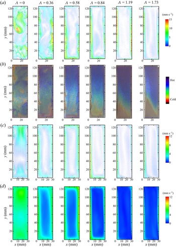
For comparison, we plot the velocity and temperature snapshots in a streamwise confined cell ( $\varGamma _x = 0.3, \varGamma _y = 1$) in figures 5(a) and 5(b). The corresponding mean velocity and r.m.s. velocity fields are shown in figures 5(c) and 5(d), respectively. The scale bars are the same as those in figure 4. It is seen that the overall flow strength is considerably lower than the spanwise confined case, and the plumes are also less vigorous than those in a spanwise confined cell. When horizontal buoyancy is zero (standard RBC), the plumes are randomly distributed in the observation plane. This is due to the fact that in such a case, the LSC lies in the
 $y\text{--}z$ plane. When an effective horizontal buoyancy is presented (
 $\varLambda \ge 0.36$), the main flow is forced into the
 $x$–
 $z$ plane, and a vertically stretched large-scale LSC is developed. Similar to the spanwise confinement case, the up-welling and down-welling flows are constrained near the sidewall and an elongated stagnant bulk region is also observed for increasing buoyancy ratio. It is also worth noting that for the streamwise confinement case, the temperature field seems do not satisfy the rotational (
 $K_{xz}$) symmetry (Zhang et al. Reference Zhang, Ding and Xia2021), which indicates that the flow is not strictly two-dimensional, and fluctuations also exist in the spanwise dimension, as with sheared RBC (Scagliarini et al. Reference Scagliarini, Gylfason and Toschi2014; Blass et al. Reference Blass, Zhu, Verzicco, Lohse and Stevens2020).
Panels (a) and (b) show experimentally measured snapshots of the velocity and temperature fields in the centre  $x$–
 $z$ plane of a streamwise confined cell (see figure 1b) for different buoyancy ratios; panels (c) and (d) show the corresponding mean velocity and r.m.s. velocity fields. The vertical Rayleigh number is fixed at
 $Ra = 10^9$ and the Prandtl number is
 $Pr = 4.3$.

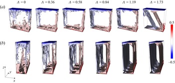
In figures 6(a) and 6(b), we plot the temperature contours in spanwise confined and streamwise confined cells with different buoyancy ratios obtained from DNS. The vertical Rayleigh number is also fixed at  $Ra_V = 10^9$. In general, the contours show similar features as the TLC images (figures 4b and 5b), and the flow in a spanwise confined cell seems more intense than the streamwise confined case. At large values of
 $\varLambda$, small-scale thermal structure survives in a spanwise confined cell but is hardly seen in a streamwise confined cell. Moreover, for the streamwise confined case, we can see several equally distantly distributed thermal streaks near the boundaries. We believe that these streaks are responsible for the breaking of rotational asymmetry observed in the liquid-crystal image (figure 5).
Numerical results. Temperature snapshots in (a) the spanwise confined cell ( $\varGamma _x = 1, \varGamma _y = 0.3$) and (b) the streamwise confined cell (
 $\varGamma _x = 0.3, \varGamma _y = 1$) for different buoyancy ratios. The vertical Rayleigh number is
 $Ra_V = 10^9$ and the Prandtl number is
 $Pr = 4.3$.

The above qualitative investigation of the flow fields reveals the key differences between the two ways of confinements: a streamwise confinement leads to a stronger inhibition of the flow strength in the plume abundant region located adjacent to the sidewalls, while a spanwise confinement leaves a larger stagnant bulk region in the centre of the convection domain.
4.2.2. Profiles at mid-height
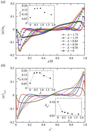
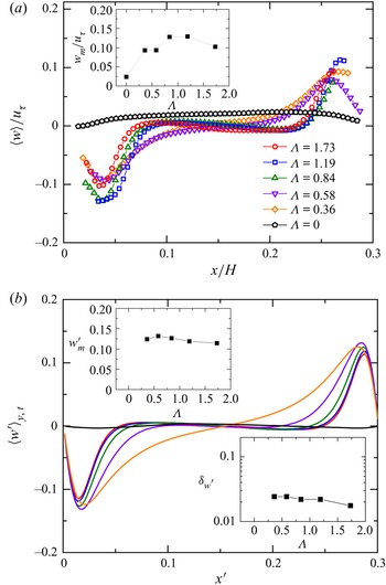
For a more quantitative examination, we first plot in figures 7(a) and 7(b) the mean vertical velocity profiles at mid-height of a spanwise confined cell obtained by experiment and DNS, respectively. The experimental data are normalized by the free fall velocity  $u_\tau = \sqrt {\alpha g\cos {\beta }{\rm \Delta} H}$. For the numerical data, an average is taken over time and the spanwise dimension. The experimental and numerical profiles show quite good agreement with each other. With increasing buoyancy ratio, the high velocity region is ‘compressed’ towards the left and right sides, and thus occupies a smaller portion of the convective domain. The maximum velocity (see the upper insets in figures 7a and 7b), on the other hand, first increases, reaching a maximum value around
 $\varLambda = 0.84$ and then decreases afterwards. The velocity BL thickness
 $\delta _{w^{\prime }}$, defined as the
 $x$-position of maximum mean vertical velocity, is plotted in the lower inset of figure 7(b). It shows a slower decrease with increasing
 $\varLambda$, and converges to a value of approximately
 $\delta _{w^{\prime }} = 0.013$ at
 $\varLambda = 1.73$.
(a) The experimentally measured mean vertical velocity profiles at the mid-height of a spanwise confined cell ( $\varGamma _x = 1, \varGamma _y = 0.3$). Different symbols correspond to different buoyancy ratios. Inset shows the maximum value of normalized mean vertical velocity; (b) the corresponding profiles obtained from DNS. The upper inset shows the maximum vertical velocity and the lower inset shows the velocity BL thickness. The vertical Rayleigh number is
 $Ra_V = 10^9$ and the Prandtl number is
 $Pr = 4.3$.

For comparison, the vertical velocity profiles in a streamwise confined cell obtained by experiment and DNS are plotted in figures 8(a) and 8(b), respectively. The scales and legends are the same as those in figure 7. Again, the experimental and numerical profiles in general agree well with each other. The small deviations between experimental and numerical profiles may be attributed to the fact that streaks are developed in such a case (see figure 6b), and the PIV measurements are only taken in the centre plane while the DNS data are averaged over the  $y$-axis. Comparing with the spanwise confined case, it is seen that the maximum vertical velocity is apparently lower at intermediate buoyancy ratios. The velocity BL thickness
 $\delta _{w^{\prime }}$, however, is slightly larger than that in the spanwise confined case.
(a) The normalized mean vertical velocity profiles measured in a streamwise confined cell ( $\varGamma _x = 0.3, \varGamma _y = 1$). The inset shows the normalized maximum mean vertical velocity; (b) the corresponding profile obtained by DNS. The upper inset shows the maximum vertical velocity and the lower inset shows the velocity BL thickness. The vertical Rayleigh number is
 $Ra_V = 10^9$ and the Prandtl number is
 $Pr = 4.3$. All the scales and legends are the same as those in figure 7.

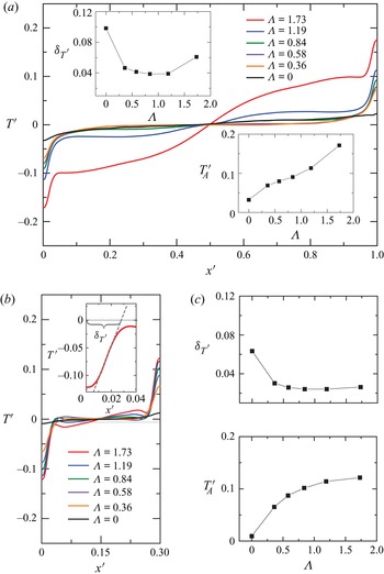
Next, we plot the DNS mean temperature profiles at the mid-height of a spanwise confined cell and a streamwise confined cell for different buoyancy ratios in figures 9(a) and 9(b), respectively. The scales and legends in figures 9(a) and 9(b) are the same. The temperature profiles typically consist of two BLs and a flat centre region that corresponds to the well-mixed bulk. The insets in figure 9(a) and figure 9(c) show the amplitude of temperature contrast  $T^\prime _A$ and the thermal BL thickness
 $\delta _{T^{\prime }}$, with the latter defined as the intercept of the tangent line with maximum slope on the
 $x$-axis (see the inset of figure 9b). It is seen that the amplitude of temperature contrast
 $T^\prime _A$ in the spanwise confined cell shows a faster increase than that in a streamwise confined cell. Another interesting point is that, for the largest buoyancy ratio
 $\varLambda = 1.73$, the mean temperature profile in a spanwise confined cell shows a non-zero slope in the centre, which is presumably due the strong stratification in the bulk (see figure 4). This stratification may also be responsible for the abrupt change in the thermal BL thickness (the last point in the upper inset of figure 9a). However, such stratification is much weaker when confinement is applied in the streamwise dimension. In such a case, the thermal BL thickness shows a slow decrease with
 $\varLambda$ while the amplitude of temperature contrast exhibits a mild increase. Furthermore, both
 $\delta _{T^\prime }$ and
 $T^\prime _A$ are smaller than those in a spanwise confined cell.
(a) The mean temperature profiles at the mid-height of a spanwise confined rectangular cell ( $\varGamma _x = 1, \varGamma _y = 0.3$) for different buoyancy ratios. The upper inset shows the thermal boundary layer thickness
 $\delta _{T^{\prime }}$ and lower inset shows the amplitude of temperature contrast
 $T^\prime _A$; (b) the corresponding profiles in a streamwise confined cell (
 $\varGamma _x = 0.3, \varGamma _y = 1$). Inset shows an example of determining the thermal BL thickness. The two subplots on the right show the thermal BL thickness and the amplitude of temperature contrast, respectively. The scales and legends in (a) and (b) are the same.

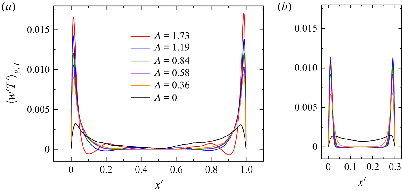
Figures 10(a) and 10(b) show the mean vertical heat flux profiles obtained by DNS at mid-height of a spanwise confined cell and a streamwise confined cell, respectively. The profiles are averaged over time and the  $y$-axis. It is clear that, when horizontal buoyancy is present (
 $\varLambda > 0$), the vertical heat flux is concentrated only in a small region near the boundaries, while the bulk region barely makes any contributions to the vertical heat transfer. The peak value of local vertical heat flux is seen to increase with the buoyancy ratio. However, the width of the ‘heat flux channels’ (areas covered by highly coherent plumes) shows little variance, if any. It is also noteworthy that the spanwise confined cell in general shows a higher peak value of local heat flux than the streamwise confined one. Nevertheless, considering the fact that in the latter case, the x-dimension is reduced by 70 %, the up-welling/down-welling flows therefore can occupy a larger portion of the convection domain. In other words, the ‘stagnant’ bulk region that makes little contribution to vertical heat transfer is to a large extent reduced by applying streamwise confinement. It is indeed the higher coverage of these ‘heat flux channels’ that leads to the net increase of heat transfer compared with the spanwise confined case.
(a) The mean vertical heat flux profiles at the mid-height of a spanwise confined cell ( $\varGamma _x = 1, \varGamma _y = 0.3$) for different buoyancy ratios; (b) the corresponding heat flux profiles in a streamwise confined cell (
 $\varGamma _x = 0.3, \varGamma _y = 1$). The vertical Rayleigh number is
 $Ra_V = 10^9$ and the Prandtl number is
 $Pr = 4.3$.

4.3. The effect of different aspect ratios
The experimental and numerical results above reveal that different aspect ratios have profound effects on the global transfer properties. However, experimentally varying the aspect ratio requires different sets of conducting plates, which is of huge cost. For this reason, we use direct numerical simulations instead to systematically explore the effects of different spanwise and streamwise aspect ratios. A brief introduction to the CUPS code is already provided in § 3. This section is further divided into four subsections. We first present in § 4.3.1 the changes in flow structures under different degrees of streamwise and spanwise confinements. Their effects on heat transport are then discussed in § 4.3.2. In § 4.3.3, we carry out a quantitative exploration of the shear strength and plume coverage, respectively. Finally, we discuss the behaviours of various streamwise profiles in § 4.3.4.
4.3.1. Flow structures
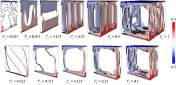
The upper and lower panels of figure 11 show the snapshots of temperature contours with varying streamwise confinement ( $\varGamma _x$) and spanwise confinement (
 $\varGamma _y$), respectively. The vertical Rayleigh number is
 $Ra_V = 10^9$ and the buoyancy ratio is fixed at
 $\varLambda = 0.84$. For the unconfined cubic cell (
 $\varGamma _x = \varGamma _y = 1$), the thermal BLs are swept directly by the LSC with the help of the horizontal buoyancy, resulting in strong shear rates at both conducting plates. As the streamwise dimension is reduced, the flow becomes more and more steady. The ‘stagnant’ bulk region is squeezed and become narrower. The cold/hot fluid descents/ascents along the sidewalls in the form of two-to-three elongated steady streaks. For the extremely confined case
 $\varGamma _x = 0.025$, such streaks break into randomly distributed small plumes and the flow becomes unsteady again. This happens when the x-dimension is comparable to twice the thickness of the thermal streaks, and the ascending hot and descending cold steaks collide with each other and break up afterwards. On the other hand, if confinement is applied in the spanwise dimension, the LSC persists even for the extremely confined cases. With decreasing
 $\varGamma _y$, the overall flow is seen to be less fluctuating due to the increased drag from the sidewalls. The wall drag also hinders turbulent mixing in the bulk region. For the lowest aspect ratio explored
 $\varGamma _y = 0.025$, the centre of the cell is stably stratified and the flow is almost laminar. In a recent study, Shishkina (Reference Shishkina2021) derived an analytical expression for the onset Rayleigh number as a function of cell aspect ratio, suggesting that for RBC (
 $\varLambda = 0$), the onset of turbulent convection is deferred by applying lateral geometrical confinement. We remark that our findings are in qualitative agreement with their predictions despite the fact that an effective horizontal buoyancy is also considered in the present study.
Snapshots of temperature fields with varying streamwise confinement (upper panel) and spanwise confinement (lower panel). The vertical Rayleigh number is  $Ra_V = 10^9$ and the buoyancy ratio is fixed at
 $\varLambda = 0.84$.

4.3.2. Heat transfer properties
In figure 12(a), we plot the vertical Nusselt number  $Nu_V$ in streamwise and spanwise confined cells as a function of aspect ratio (degree of confinement) using red circles and blue triangles, respectively. For reference, the Nusselt number in a non-tilted RB cell (
 $\varLambda = 0$) is also plotted as black diamonds (Huang et al. Reference Huang, Kaczorowski, Ni and Xia2013; Huang & Xia Reference Huang and Xia2016). The open symbols represent the DNS data, and the solid circles are the experimental data. The heat transfers in these two confinement settings show no apparent difference when
 $\varGamma _x, \varGamma _y \ge 0.5$, for which the confinement effect is not significant. Nevertheless, a considerable enhancement in
 $Nu_V$ is observed for moderate aspect ratios (
 $0.075 \le \varGamma _x, \varGamma _y \le 0.3$), and curve of
 $Nu_V$ for the streamwise confined case lays on top of the spanwise confined one. The experimental data are also in agreement with this finding. The upward shift of the experimental data is presumably due to the inevitable heat leakage. For the severely confined case, all three curves show abrupt decreases in
 $Nu_V$. For the lowest aspect ratio, the
 $Nu_V$ of the streamwise confined cell is even lower than that of the spanwise confined cell. We attribute this to the breakup of coherent streaks (see figure 11). We then plot in figure 12(b) the corresponding normalized vertical Nusselt number. It is evident that the streamwise confinement shows a higher enhancement in heat transfer, except for the point with lowest aspect ratio. The normalized experimental and numerical data also show very good agreement. The maximum enhancement in
 $Nu_V$ reaches approximately 35 % for streamwise confinement with
 $\varGamma _x = 0.05$.
(a) Vertical Nusselt number  $Nu_V$ as a function of different aspect ratios
 $\varGamma _x$ and
 $\varGamma _y$. Solid symbols represent the experimental data and open symbols are the DNS data. Red circles and blue triangles denote streamwise and spanwise confined cells with buoyancy ratio
 $\varLambda = 0.84$, respectively. The black diamonds correspond to
 $\varLambda = 0$. The error bars denote the temporal fluctuations of
 $Nu_V$; (b) normalized vertical Nusselt number as a function of the streamwise/spanwise aspect ratio, the legends are the same as those in (a). The vertical Rayleigh number is
 $Ra_V = 10^8$ and the Prandtl number is
 $Pr = 4.3$.

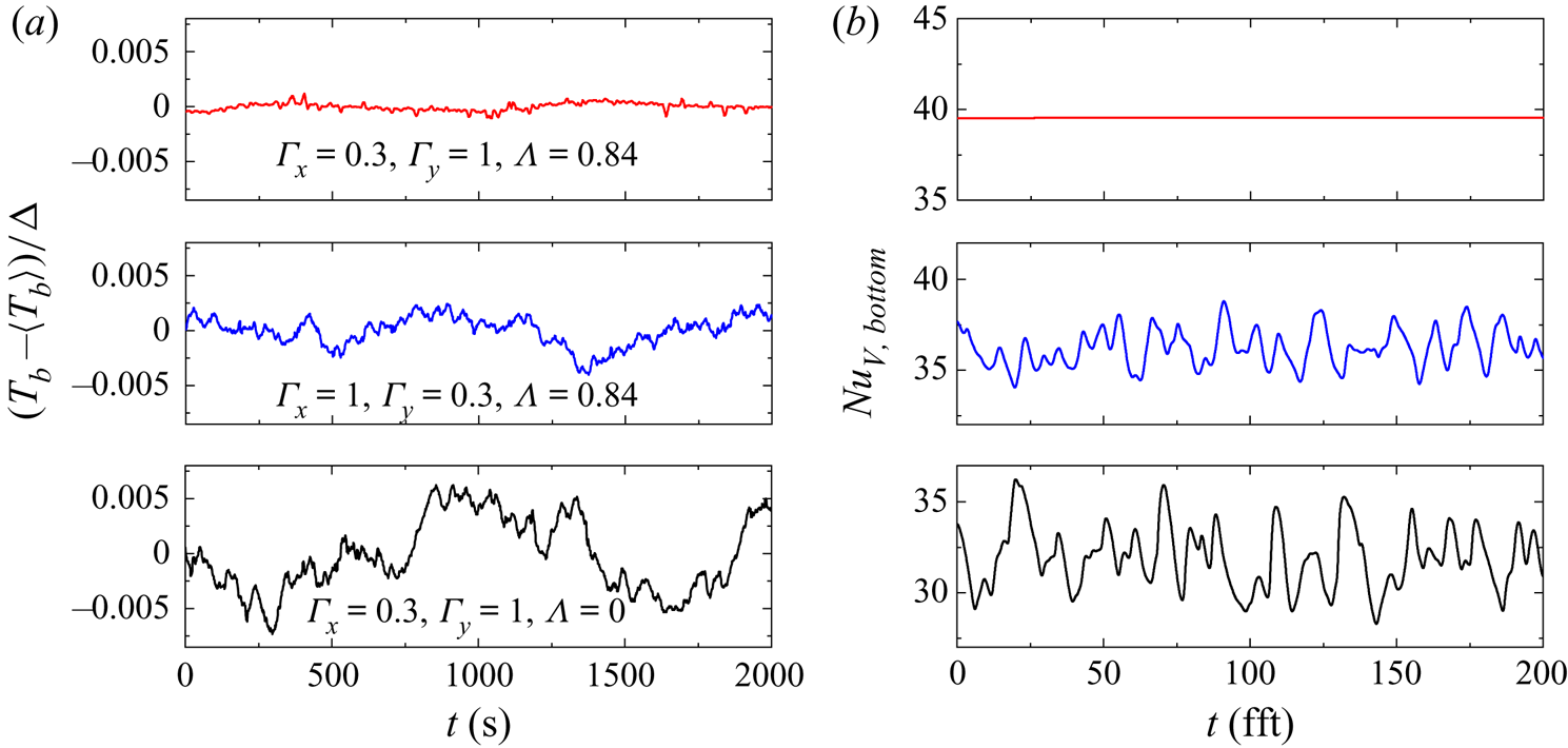
The error bars in figure 12(a) show the standard deviation of instantaneous  $Nu_V$. A close inspection of the data reveals that streamwise confinement leads to a stronger inhibition of heat transfer fluctuation than spanwise confinement. For a clearer view of this point, we plot in figure 13(a) the experimentally measured normalized bottom plate temperature series
 $(T_b-\langle T_b\rangle )/\varDelta$. When no horizontal buoyancy is present (
 $\varLambda = 0$, the lower panel), the bottom plate temperature shows strong random fluctuations. Whereas a buoyancy ratio of
 $\varLambda = 0.84$ will significantly suppress the temperature fluctuation, and the streamwise confinement case (
 $\varGamma _x = 0.3, \varGamma _y = 1$) shows a smaller amplitude of fluctuation than the spanwise confinement case (
 $\varGamma _x = 1, \varGamma _y = 0.3$), indicating a more steady flow in such configuration. It is worth mentioning that, strictly speaking, the bottom plate temperature boundary conditions in the experiment and DNS are different, with the former being close to a constant flux boundary condition and the latter being a constant temperature boundary condition (Verzicco & Sreenivasan Reference Verzicco and Sreenivasan2008; Huang et al. Reference Huang, Wang, Xi and Xia2015). Therefore, with the numerical data, we plot in figure 13(b) the instantaneous vertical Nusselt number
 $Nu_{V,b}$ at the bottom plate from DNS instead. Nevertheless, the fluctuations of
 $Nu_{V,b}$ show similar behaviour as the experimentally measured bottom temperature fluctuations. For the streamwise confined case, the vertical Nusselt number at bottom plate is constant, suggesting that the flow is laminar, which further confirms the fact that streamwise confinement is more efficient in inhibiting turbulence than spanwise confinement.
(a) Time series of the experimentally measured bottom plate temperature in, from top to bottom, a streamwise confined cell ( $\varGamma _x = 0.3, \varGamma _y = 1, \varLambda = 0.84$), a spanwise confined cell (
 $\varGamma _x = 1, \varGamma _y = 0.3, \varLambda = 0.84$) and a standard RB cell (
 $\varGamma _x = 0.3, \varGamma _y = 1, \varLambda = 0$); (b) time series of the bottom plate Nusselt number obtained by DNS. The legends are the same as those in (a).

4.3.3. Shear strength and plume coverage
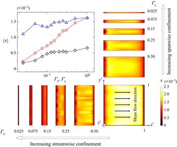
As mentioned in § 1, there are two possible mechanisms that are responsible for the enhancement of vertical heat transfer in the present system: one is the increased shear at the boundaries resulting from the applied effective horizontal buoyancy, the other is the lateral confinement induced plume coverage increase and coherent structure condensation. In the following, we will examine these two effects in turn to determine their contributions to the overall heat transfer. We first plot in the upper-left panel of figure 14 the surface averaged mean shear rates  $\langle \tau \rangle$ at the bottom plates of cells with different streamwise (red circles) and spanwise (blue triangles) confinements. The vertical Rayleigh number is
 $Ra_V = 10^8$ and the buoyancy ratio is also fixed at
 $\varLambda = 0.84$. For comparison, we also plot the mean bottom plate shear rates in a ‘levelled’ RB cell using black diamonds. It is seen that the presence of an effective horizontal buoyancy will significantly increase the mean shear rate. Meanwhile, all three curves in general decrease with increasing lateral confinement, which is expected since a spanwise confinement will increase the wall drag and a streamwise confinement directly restricts the development of streamwise flow. It is noteworthy that the curve for streamwise confinement always lies below the spanwise confined one. This suggests that, compared with the spanwise confined case, the moderate increase in shear rate in a streamwise confined cell cannot be responsible for the observed rapid vertical heat transfer enhancement (see figure 12).
Upper-left panel, mean shear rates  $\langle \tau \rangle$ at the bottom plate (
 $z^\prime = 0$) for different confinement settings. The red circles and blue triangle denote data from streamwise confined and spanwise confined cells with a buoyancy ratio of
 $\varLambda = 0.84$, respectively. The black diamonds represent cells with
 $\varLambda = 0$. For reference, the mean shear rates at the bottom plate under different streamwise and spanwise confinements are plotted in the bottom row and right column, respectively. The vertical Rayleigh number is
 $Ra_V = 10^8$ and the Prandtl number is
 $Pr = 4.3$.

To offer a more intuitive view of the shear strength, we also plot in the right column and the bottom row of figure 14 the mean bottom plate shear rates in spanwise confined and streamwise confined cells, respectively. It is seen that spanwise confinement reduces the shear rate near the front and back lateral walls (top and bottom boundaries from top view as in figure 14), while for the lowest aspect ratio explored ( $\varGamma _y = 0.025$), a highlighted region with strong horizontal shear can still be observed in the centre of the bottom plate. On the contrary, a streamwise confinement restrains the development of horizontal shear in the bottom plane, therefore the highlighted region with strong shear gradually diminishes with decreasing
 $\varGamma _x$.
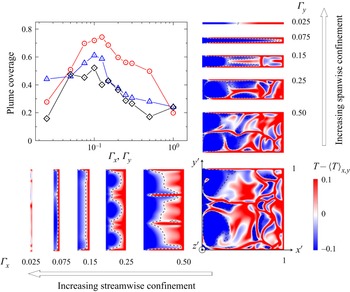
The second possible mechanism is the increase in plume coverage and coherency. Zhang et al. (Reference Zhang, Ding and Xia2021) reported that the effective horizontal buoyancy will ‘push’ the hot plumes towards the right end and ‘pull’ the cold plumes to the left end, thus separating the hot and cold plumes and therefore increasing the coherency of the flow. For a more quantitative view of the plume coverage, we adopt the definition proposed in Chong et al. (Reference Chong, Huang, Kaczorowski and Xia2015), i.e. any region fulfils the criterion  $\pm (T-\langle T\rangle _{x,y}) > cT_{rms}$ is considered to be covered by hot/cold plumes. Here,
 $c$ is an empirical parameter and we take the value
 $c = 1$. With this, we plot in figure 15 the mean plume coverage as a function of the aspect ratio. The legends are the same as those in figure 14. The snapshots of spatial temperature fluctuations (
 $T-\langle T\rangle _{x,y}$) in the horizontal cross-section that is one thermal BL thickness away from the bottom plate (
 $z^\prime = \delta _{T^{\prime }}$) are also plotted for reference. We can see that the plume coverage shows a significant increase when a horizontal buoyancy is present (
 $\varLambda = 0.84$) for both confinement settings. Most importantly, we can see that the streamwise confined cell shows a significantly higher plume coverage than the spanwise confined one, except for the point with the lowest aspect ratio, which is probably due to the breakup of coherent structures. The maximum plume coverage reaches over 70 % at a streamwise confinement of
 $\varGamma _x = 0.025, \varGamma _y = 1$. Combining the above findings with the observations in § 4.2.1, we can infer that, for
 $\varGamma _x \ge 0.125$, the main effect of streamwise confinement is to decrease the volume of stagnant bulk region, whereas the volumes of descending(ascending), cold(hot) flows that developed adjacent to the vertical sidewalls are almost unaffected (see figure 11). Since the area of the conducting plates decreases with decreasing
 $\varGamma _x$, these coherent structures can thus impinge on a larger portion of the bottom (top) plate (see the dashed lines in figure 15), resulting in an increase in the plume coverage. While for
 $\varGamma _x < 0.125$, the convection domain is almost occupied entirely by the downward/upward moving plumes and a further decrease in
 $\varGamma _x$ will constrain their streamwise dimension, therefore a reduction in plume coverage is observed.
Upper-left panel, the mean plume coverage near the bottom plate of cells with different confinement settings. The red circles and blue triangles denote data from streamwise confined and spanwise confined cells with a buoyancy ratio  $\varLambda = 0.84$, respectively. The black diamonds represent standard RBC (
 $\varLambda = 0$). The snapshots of temperature fluctuations
 $T-\langle T\rangle _{x,y}$ in a horizontal cross-section located at one thermal BL thickness
 $z^\prime = \delta _{T^{\prime }}$ above the bottom plate under different streamwise and spanwise confinements are plotted in the bottom row and right column, respectively. The dashed lines denote areas covered by the cold plumes. The vertical Rayleigh number is
 $Ra_V = 10^8$ and the Prandtl number is
 $Pr = 4.3$.

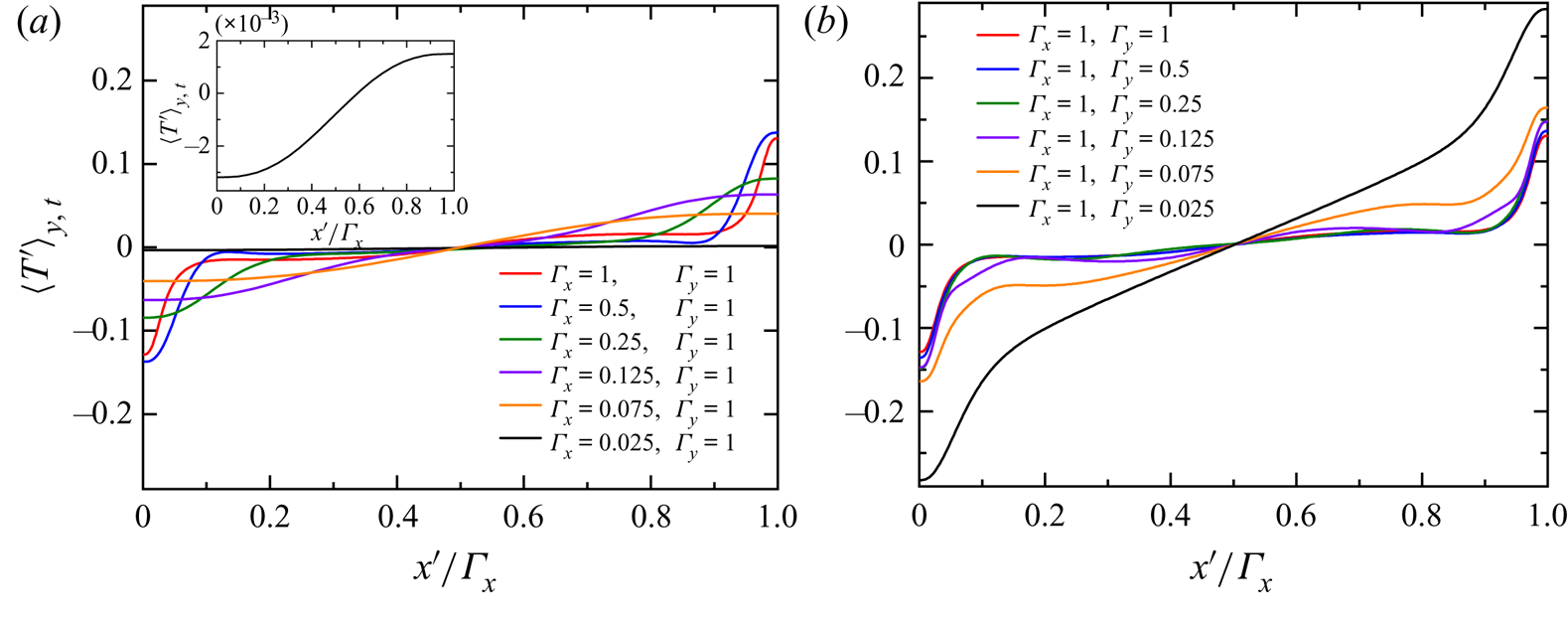
(a) The spanwise averaged mean temperature profiles as functions of normalized streamwise position  $x^\prime /\varGamma _x$ at mid-height of cells with different streamwise confinements. The inset shows a magnified view of the case with
 $\varGamma _x = 0.025$; (b) the corresponding mean temperature profiles with different spanwise confinements. The buoyancy ratio is
 $\varLambda = 0.84$. The vertical Rayleigh number is
 $Ra_V = 10^8$ and the Prandtl number is
 $Pr = 4.3$.

We now summarize the above important findings as follows. Firstly, the effect of lateral confinement in a rectangular cell is twofold: on one hand, it will decrease the shear rate on both plates created by the effective horizontal buoyancy; on the other hand, it can increase the plume coverage. Secondly, the increase in plume coverage and the decrease of shear rate in a streamwise confined cell are both faster than those in a spanwise confined cell. Therefore, albeit at a cost of lowering the shear rate, the increased plume coverage in a streamwise confined cell leads to a net increase in  $Nu_V$. We conclude that, for turbulent thermal convection systems, promoting the coherency of the flow is more efficient in enhancing the global transfer than increasing the shear rate at the boundary.
4.3.4. The properties of streamwise profiles
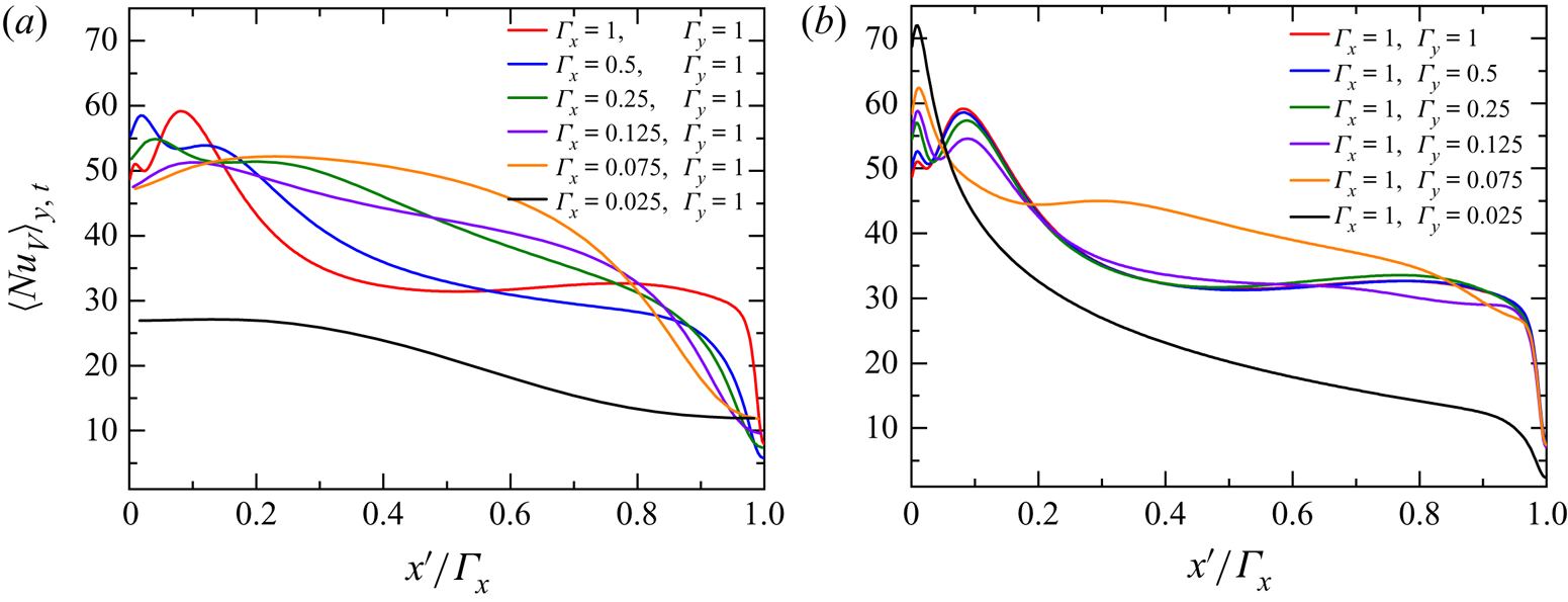
Next, we examine the effects of lateral confinement on the velocity, temperature as well as the local heat flux profiles, respectively. In figures 16(a) and 16(b), we plot the spanwise averaged mean temperature profiles  $\langle T^\prime \rangle _{y,t}$ at mid height of a streamwise confined cell and a spanwise confined cell, respectively. The horizontal position
 $x^\prime$ is normalized by the streamwise aspect ratio
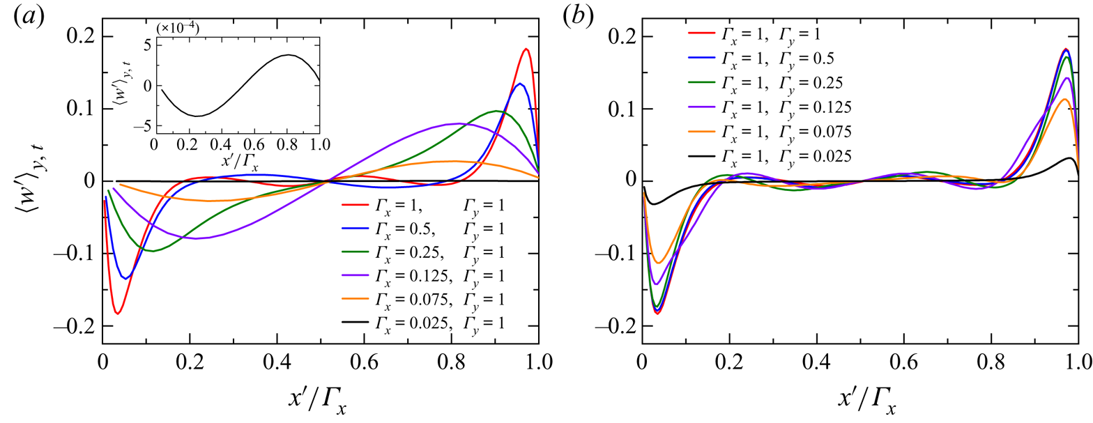
 $\varGamma _x$. Interestingly, we find that the temperature contrast at both ends of the sidewall is suppressed in a streamwise confined cell but enhanced in a spanwise confined one. With decreasing streamwise dimension, the well-mixed bulk region shrinks and finally disappears. On the other hand, a spanwise confinement will instead increase the temperature slope in the bulk region, which indicates that the flow is weakened and no longer well mixed in the centre. This fact can also be verified by figures 17(a) and 17(b), in which we plot the corresponding vertical velocity profiles. Confinement in either streamwise or spanwise dimension results in a reduction in the vertical velocity. Furthermore, it is now evident that a streamwise confinement will significantly reduce the coverage of the ‘quiescent’ bulk region, while a spanwise confinement barely has any effect on it.
(a) The spanwise averaged mean vertical velocity profiles as functions of normalized streamwise position  $x^\prime /\varGamma _x$ at mid-height of cells with different streamwise confinements; (b) the corresponding mean vertical velocity profiles in spanwise confined cells.

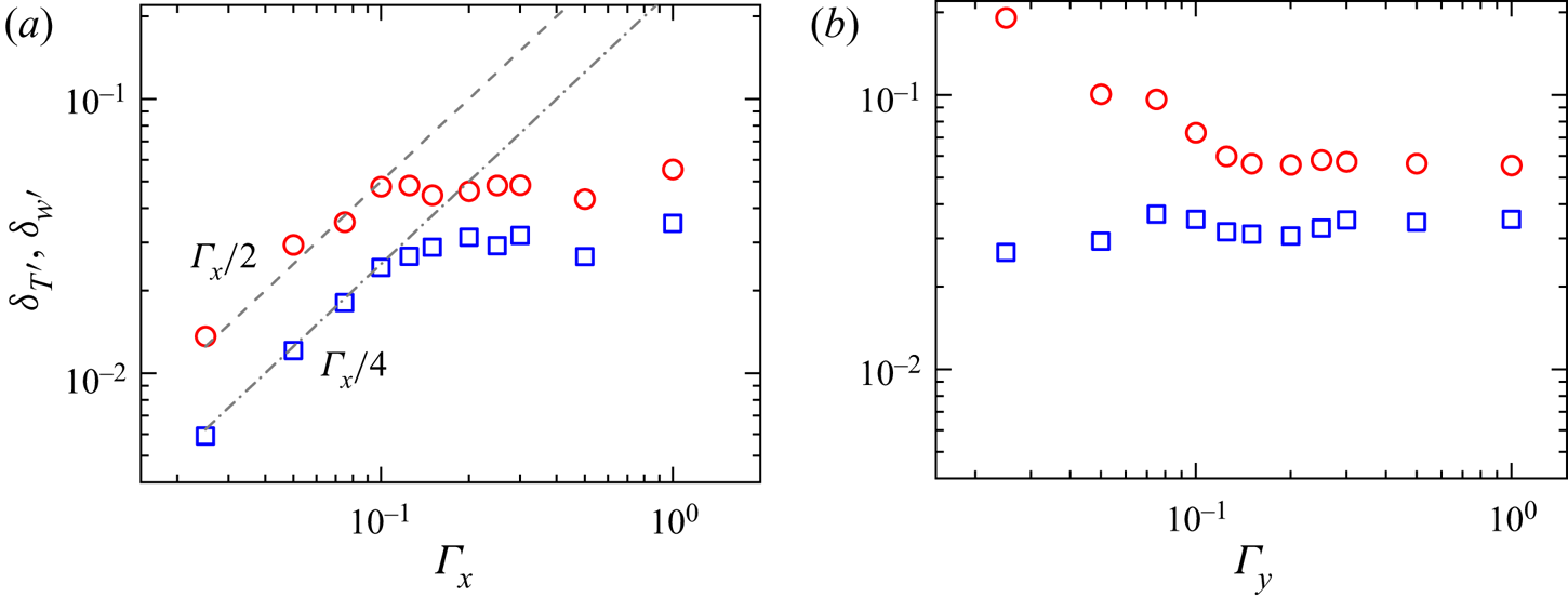
For a more quantitative view, we plot in figures 18(a) and 18(b) the thermal BL thickness  $\delta _{T^{\prime }}$ and the velocity BL thickness
 $\delta _{w^{\prime }}$ for two confinement configurations using red circles and blue squares, respectively. The definition of
 $\delta _{T^{\prime }}$ is the same as that in figure 9. The velocity boundary layer thickness
 $\delta _{w^{\prime }}$ is defined as the x-position with maximum vertical velocity. For both streamwise and spanwise confinements, the thermal and viscous BL thicknesses show little variation for
 $\varGamma _x, \varGamma _y \ge 0.15$. Whereas when the streamwise dimension
 $\varGamma _x$ is smaller than 0.15,
 $\delta _{T^{\prime }}$ and
 $\delta _{w^{\prime }}$ decrease linearly as
 $\varGamma _x/2$ and
 $\varGamma _x/4$, which are the maximum temperature and velocity BL thicknesses, respectively. This implies that, in this regime, the whole convection domain is indeed occupied by the up-welling and down-welling coherent structures that are responsible for the vertical heat transfer. In other words, the ‘stagnant’ bulk region that makes no contribution to
 $Nu_V$ is eliminated, so the overall vertical heat transfer is more efficient. When the spanwise dimension
 $\varGamma _y$ is smaller than 0.15, the velocity BL thickness only shows a slight decrease with
 $\varGamma _y$, while the thermal BL thickness, on the contrary, grows with decreasing
 $\varGamma _y$. This is again due to the fact that in this regime the bulk is not well mixed and a stably stratified temperature gradient is built therein, while in the definition of
 $\delta _{T^{\prime }}$, we have used the intercept of tangent line at the x-axis (
 $T^\prime = 0$), and such a definition implicitly requires that the bulk is well mixed. The boundary layer thicknesses
 $\delta _{T^{\prime }}$ and
 $\delta _{w^{\prime }}$ can, to some extent, describe how much area of the domain is involved in efficient vertical heat transfer. On the other hand, the temperature contrast
 $T^\prime _A$ as well as the maximum vertical velocity
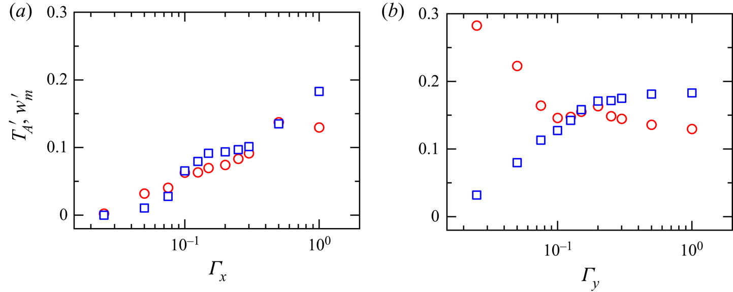
 $w^\prime _m$ are closely related to the strength of convective vertical heat flux. In figures 19(a) and 19(b), we plot
 $T^\prime _A$ and
 $w^\prime _m$ as functions of
 $\varGamma _x$ and
 $\varGamma _y$ in a streamwise confined and a spanwise confined cell, respectively. It is seen that an increase in streamwise confinement (decreasing
 $\varGamma _x$) will reduce both the amplitude of temperature contrast and the maximum vertical velocity. In contrast, spanwise confinements have only marginal effects on
 $T^\prime _A$ and
 $w^\prime _m$ for
 $\varGamma _y \ge 0.15$, which is consistent with the behaviour of
 $\delta _{T^{\prime }}$ and
 $\delta _{w^{\prime }}$ (see figure 18b). When the spanwise aspect ratio
 $\varGamma _y$ is smaller than 0.15, the maximum vertical velocity decreases rapidly with decreasing
 $\varGamma _y$, while the amplitude of temperature deviation
 $T^\prime _A$ shows an abrupt increase instead, reaching a value approximately
 $T^\prime _A = 0.3$ at the lowest aspect ratio explored (
 $\varGamma _y = 0.025$). This counter-intuitive increase in
 $T^\prime _A$ is probably due to the condensation of coherent structures (Chong et al. Reference Chong, Huang, Kaczorowski and Xia2015).
(a) The thermal BL thickness  $\delta _{T^\prime }$ (red circles) and the viscous BL thickness
 $\delta _{w^\prime }$ (blue squares) at mid-height of the sidewall for different streamwise confinements. The dashed line shows a guideline of
 $\varGamma _x/2$ and the dash-dotted line shows a guideline of
 $\varGamma _x/4$; (b) the corresponding thermal and viscous BL thicknesses in a spanwise confined cell. The buoyancy ratio is
 $\varLambda = 0.84$. The vertical Rayleigh number is
 $Ra_V = 10^8$ and the Prandtl number is
 $Pr = 4.3$.

(a) The amplitude of the temperature deviation  $T^\prime _A$ (red circles) and the maximum vertical velocity
 $w_m^\prime$ at mid-height of the sidewall in a streamwise confined cell; (b) the corresponding temperature deviation and maximum vertical velocity in a spanwise confined cell. The buoyancy ratio is
 $\varLambda = 0.84$ in both cases.

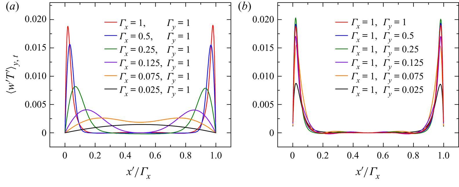
In figures 20(a) and 20(b), we plot the spanwise averaged convective vertical heat flux profiles  $\langle w^\prime T^\prime \rangle _{y,t}$ at mid-height of cells with streamwise confinement and spanwise confinement, respectively. Most of the profiles show bimodal distributions, with the two peaks located near the left and right ends of the sidewalls, as expected. It is also clear that streamwise confinement reduces the magnitude of local heat flux but increases the effective area of vertical heat transfer; while a spanwise confinement only effects the magnitude of local heat flux. We also note that, when the streamwise dimension is smaller than a critical value, the two peaks start to merge with each other and finally condense to form a single peak. This happens when the coherent thermal streaks breakup into plumes (see figure 11) and is concurrent with a sharp reduction in
 $Nu_V$.
The profiles of spanwise averaged vertical heat flux as a function of normalized streamwise position at mid-height of cells with (a) streamwise confinements and (b) spanwise confinements. The vertical Rayleigh number is  $Ra_V = 10^8$ and the buoyancy ratio is
 $\varLambda = 0.84$ for both cases. The Prandtl number is
 $Pr = 4.3$.

In the last part of this section, we will discuss the behaviours of the mean shear rate and local heat flux at the bottom plate under different confinement settings. Figures 21(a) and 21(b) show the mean profiles of shear rate in a streamwise confined cell and a spanwise confined cell, respectively. As above, average is taken over the y-axis. When the streamwise dimension  $\varGamma _x$ is larger than 0.5,
 $\langle \tau \rangle _{y,t}$ shows a plateau in the centre region of the cell, suggesting that the horizontal shear is nearly fully developed with the help of effective horizontal buoyancy. However, for
 $\varGamma _x \le 0.25$, such a plateau disappears and the mean shear profile is featured by a single bump with deceasing amplitude. This implies that, in such a situation, the horizontal buoyancy can only force the LSC into the
 $x$–
 $z$ plane but is not able to fully accelerate its horizontal motion. On the contrary, the centre plateau is always present in a cell with spanwise confinement. In such a case, a little bump is discernible at a streamwise position around
 $x^\prime = 0.15$ for
 $\varGamma _y \ge 0.125$, which is presumably due to the impingement of cold plumes. Meanwhile, all profiles show little skew to the left. A decrease in
 $\varGamma _y$ only reduces the magnitude of the profile while its shape is in general unchanged.
The mean shear rate at the bottom plate as a function of normalized streamwise position  $x^\prime$ in (a) streamwise confined cells and (b) spanwise confined cells. The buoyancy ratio is
 $\varLambda = 0.84$.

The distributions of local heat flux are more complicated, as shown in figures 22(a) and 22(b). For all cases considered, the profiles are highly asymmetric, with the highest  $Nu_V$ locates near the left boundary. This asymmetry results from the applied horizontal buoyancy and directly accounts for a global horizontal heat transfer (Zhang et al. Reference Zhang, Ding and Xia2021). The location of maximum local
 $Nu_V$ corresponds to the position where the downward cold plumes impinge on the bottom plate. After reaching its maximum, the local heat flux then shows a gradual decrease towards the right end, and finally drops rapidly to zero. For the streamwise confined case, no plateau is observed (note that the red curve corresponds to the unconfined case
 $\varGamma _x = \varGamma _y = 1$). While for the spanwise confined case, the local heat flux shows a plateau in the central region for
 $\varGamma _y \ge 0.125$. This plateau may serve as a signal of the fully developed horizontal shear flow. When such a plateau is present, a close inspection of the left region of the profile reveals a double peak distribution, indicating the existence of a weak secondary flow in the corner. For the unconfined case (
 $\varGamma _x = \varGamma _y = 1$), the second peak is the global maximum. Decreasing the spanwise dimension
 $\varGamma _y$ will lower the second peak and raise the first one. At
 $\varGamma _y = 0.125$, the first peak takes over the second one, becomes the global maximum. As we further decrease
 $\varGamma _y$, the second peak eventually disappears. We remark that, the complex behaviours of local shear and local heat transfer properties above pose a challenge in developing a theory that incorporates the aspect ratio dependence of turbulent thermal convection in the presence of effective horizontal buoyancy. Such a theory should at least reproduce the essential features discussed above, which is beyond the scope of this paper, but certainly deserves future studies.
The spanwise averaged vertical Nusselt number as a function of the normalized streamwise position  $x^\prime /\varGamma _x$ in (a) streamwise confined cell and (b) spanwise confined cell. The vertical Rayleigh number is
 $Ra_V = 10^8$ and the buoyancy ratio is
 $\varLambda = 0.84$.

5. Energetics and mixing efficiency
Complicated as the effect of aspect ratio is, a theoretical treatment from the perspective of energetics is, however, feasible. In this section, we will first discuss the energetics of thermal convection in the presence of an effective horizontal buoyancy, and then explore the effects of different aspect ratios accordingly. The concept of energetics in thermal convection system is first raised by Winters et al. (Reference Winters, Lombard, Riley and DÁsaro1995) for density-stratified fluid flows and later generalized to RBC by Hughes, Gayen & Griffiths (Reference Hughes, Gayen and Griffiths2013) and Gayen, Hughes & Griffiths (Reference Gayen, Hughes and Griffiths2013). The central idea of the framework is to separate the available potential energy from the background potential energy. With the presence of an effective horizontal buoyancy, the specific total potential energy can be written as  $E_p = (\cos {\beta }g/\rho _0)\langle z\rho \rangle_V + (\sin {\beta }g/\rho _0)\langle x\rho \rangle_V$. And the specific background potential energy is
 $E_b = (\cos {\beta }g/\rho _0)\langle z^\ast \rho \rangle_V + (\sin {\beta }g/\rho _0)\langle x^\ast \rho \rangle_V$, where
 $x^\ast$ and
 $z^\ast$ are the horizontal and vertical positions of a fluid parcel when it was adiabatically rearranged to the ‘ground state’ with minimal potential energy. The difference between
 $E_p$ and
 $E_b$ is just the specific available potential energy
 $E_a = E_p - E_b$. The specific kinetic energy, as usual, can be defined as
 $E_k = \langle u^2+v^2+w^2\rangle _V/2$. The definitions above are based on the density field
 $\rho$. For the present study, we can easily express the potential energies in terms of temperature
 $T$ using the Oberbeck–Boussinesq approximation,
 $(\rho -\rho _0)/\rho _0 = -\alpha (T-T_0)$. In a dynamical system, different forms of mechanical energy can transform from each other. For example, the horizontal buoyancy flux (
 $\varPhi _x = (g/\rho _0)\langle \rho u\rangle _V$) and vertical buoyancy flux (
 $\varPhi _z = (g/\rho _0)\langle \rho w\rangle _V$) transform the available potential energy to the kinetic energy. Meanwhile, the irreversible mixing rate
 $\varPhi _d$ and the background molecular diffusion rate
 $\varPhi _i$ can be expressed as
 \begin{gather} \varPhi_d ={-} \frac{\kappa \cos\beta g}{\rho_0}\langle({\rm d}z^\ast{/}{\rm d}\rho)(\boldsymbol{\nabla}\rho)^2\rangle_V -\frac{\kappa\sin\beta g}{\rho_0}\langle({{\rm d}\kern0.7pt x}^\ast{/}{\rm d}\rho)(\boldsymbol{\nabla}\rho)^2\rangle_V, \end{gather}
 \begin{gather}\varPhi_i ={-} \frac{\kappa \sin\beta g}{\rho_0}\frac{\varDelta\langle\rho\rangle_{A_{x}}}{\varDelta_x} - \frac{\kappa \cos\beta g}{\rho_0}\frac{\varDelta\langle\rho\rangle_{A_{z}}}{\varDelta_z}. \end{gather}
For the present system, heat is injected through the hot bottom plate and removed from the cold top plate, thus continuously inputting potential energy into the system. We can then obtain the energy input rates for total specific potential energy and background specific potential energy as
 \begin{gather} \varPhi_{b1} = \frac{\kappa \cos\beta g}{\rho_0V}\oint z \boldsymbol{\nabla}\rho\boldsymbol{\cdot} {\rm d} \boldsymbol{S} + \frac{\kappa \sin \beta g}{\rho_0V}\oint x \boldsymbol{\nabla}\rho\boldsymbol{\cdot} {\rm d} \boldsymbol{S}, \end{gather}
 \begin{gather}\varPhi_{b2} ={-} \frac{\kappa \cos\beta g}{\rho_0V}\oint z^\ast\boldsymbol{\nabla}\rho\boldsymbol{\cdot} {\rm d} \boldsymbol{S} - \frac{\kappa \sin\beta g}{\rho_0V}\oint x^\ast\boldsymbol{\nabla}\rho\boldsymbol{\cdot} {\rm d} \boldsymbol{S}. \end{gather}
Replacing density  $\rho$ with temperature
 $T$, and using the definition for horizontal and vertical Nusselt numbers (Zhang et al. Reference Zhang, Ding and Xia2021), we can obtain
 \begin{gather} \varPhi_{b1} = Nu_V(\alpha{\rm \Delta} T/H)\kappa\cos\beta g + Nu_H(\alpha{\rm \Delta} T/H)\kappa\sin\beta g, \end{gather}
 \begin{gather}\varPhi_{b2} = Nu_V(\alpha{\rm \Delta} T/H)\kappa\cos\beta g + \varGamma_xNu_V(\alpha{\rm \Delta} T/H)\kappa\sin\beta g, \end{gather}
 \begin{gather}\varPhi_{i} ={-}(\alpha{\rm \Delta} T/H)\kappa\cos\beta g - [\alpha(\langle T\rangle_{x=0}-\langle T\rangle_{x=\varGamma_{x}})/(\varGamma_xH)]\kappa\sin\beta g, \end{gather}
where  $\varGamma _x$ is just the streamwise aspect ratio of the convection domain. When the system is in a statistical stationary state, the ensemble average of the time derivative of all forms of mechanical energy should equal to zero
 \begin{gather} \left\langle\frac{{\rm d}E_k}{{\rm d}t}\right\rangle = \langle-\varPhi_x-\varPhi_z-\epsilon\rangle = 0, \end{gather}
 \begin{gather}\left\langle\frac{{\rm d}E_a}{{\rm d}t}\right\rangle = \langle\varPhi_x+\varPhi_z+\varPhi_{b1}+\varPhi_{b2}-\varPhi_d+\varPhi_{i}\rangle = 0, \end{gather}
 \begin{gather}\left\langle\frac{{\rm d}E_b}{{\rm d}t}\right\rangle = \langle-\varPhi_{b2}+\varPhi_d\rangle = 0. \end{gather}
Combining (5.5)–(5.10), we can obtain the final expression for the mixing efficiency  $\eta$, defined as the ratio between the energy used for diapycnal mixing and all irreversible energy transfer
 \begin{align} \eta &= \left\langle\frac{\varPhi_d-\varPhi_i}{\varPhi_d-\varPhi_i+\epsilon}\right\rangle\nonumber\\ &= \left\langle\frac{\varPhi_{b2}-\varPhi_i}{\varPhi_{b2}+\varPhi_{b1}}\right\rangle = \frac{1+\varLambda\varGamma_x + Nu_V^{{-}1} + \varLambda(\langle T\rangle_{x=0}-\langle T\rangle_{x=\varGamma_{x}})\varGamma_x^{{-}1}Nu_V^{{-}1}}{2+\varLambda\varGamma_x + \varLambda Nu_H/Nu_V} \nonumber\\ &\approx \frac{1+\varLambda\varGamma_x}{2+\varLambda\varGamma_x+\varLambda Nu_H/Nu_V}. \end{align}
In the last step of (5.11), we have omitted the last two terms in the numerator since, for the Rayleigh number range considered,  $Nu_V^{-1} \ll 1$. Note that when
 $\varLambda = 0$, (5.11) reduces to the
 $\eta = 1/2$ limit for RBC (Hughes et al. Reference Hughes, Gayen and Griffiths2013). It is also worth mentioning that the value of 1/2 also serves as a lower bound for
 $\eta$, since
 $Nu_H/Nu_V < \varGamma _x$. Moreover, considering that
 $\varGamma _x$ and
 $\varLambda$ are both control parameters, it is indeed the ratio between the horizontal Nusselt number and vertical Nusselt number
 $Nu_H/Nu_V$, i.e. the orientation of the global heat transfer that determines the mixing efficiency of the system.
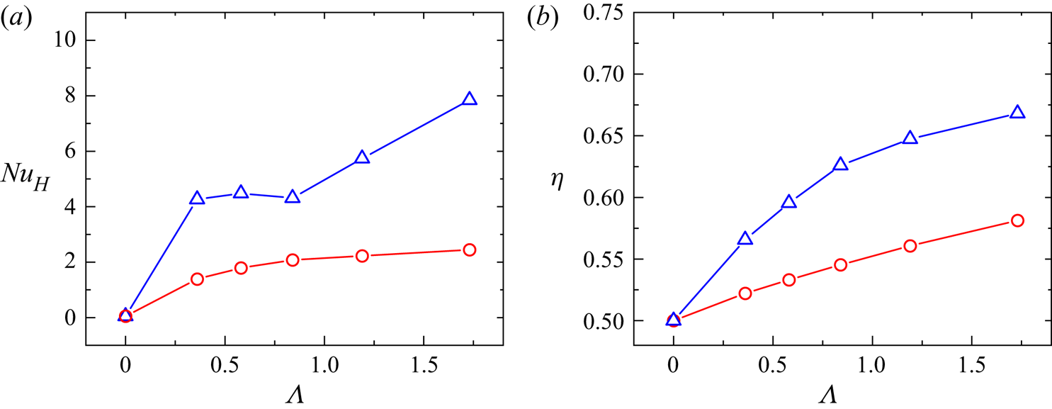
In figure 23(a), we plot the horizontal Nusselt number obtained by DNS as a function buoyancy ratio  $\varLambda$. The red circles represent data from a streamwise confined cell and the blue triangles are data from a spanwise confined cell. It is seen that the horizontal Nusselt number in the spanwise confined cell is always larger than that in the streamwise confined cell. This is expected since the amplitude of
 $Nu_V$ is limited by the horizontal (streamwise) scale of the convective domain. Combining this with the results of vertical Nusselt number (see figure 3), we may conclude that the enhancement in vertical Nusselt number by streamwise confinement is accompanied by a ‘sacrifice’ in the horizontal heat transfer. We then plot the corresponding mixing efficiency in figure 23(b). It is seen that for both confinement settings, the mixing efficiencies show monotonic increases with the buoyancy ratio, reaching maximum values of 0.67 and 0.58 for spanwise confinement and streamwise confinement at
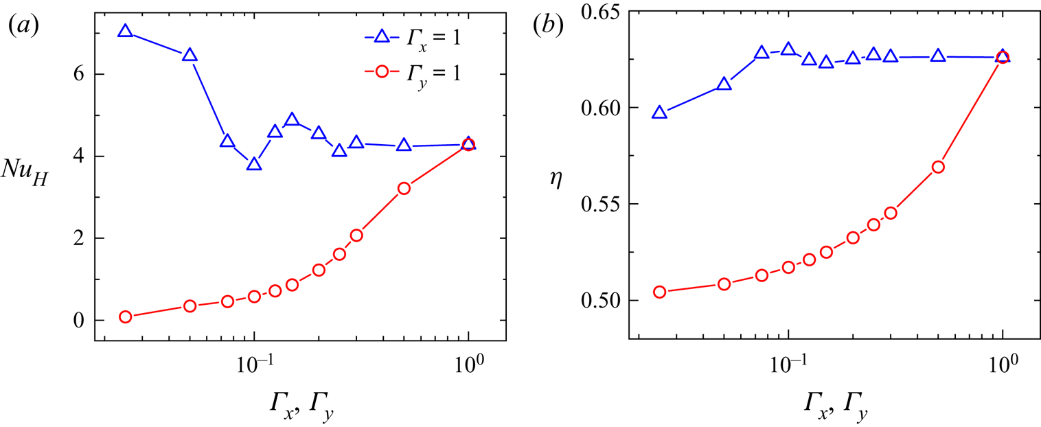
 $\varLambda = 1.73$, respectively. Finally, we explore the effect of different aspect ratios by plotting the horizontal Nusselt number and mixing efficiency as a function of
 $\varGamma _x$ and
 $\varGamma _y$ in figures 24(a) and 24(b), respectively. It is seen that, with increasing streamwise confinement, the horizontal Nusselt number shows a rapid decrease since it is inherently limited by the horizontal scale of the domain. While a spanwise confinement results in a mild increase in the horizontal heat transfer. We do not know the exact reason for such increase yet, it may be related to the reduction of turbulent fluctuation (see the lower panel of figure 11), i.e. the adverse spanwise fluctuation for horizontal (and vertical) heat transport is, to a large extend, suppressed by applying a spanwise confinement. The mixing efficiency
 $\eta$ shows similar behaviour as the horizontal Nusselt number
 $Nu_H$, it decreases rapidly with increasing streamwise confinement, approaching the 1/2 lower bound for
 $\varGamma _x \rightarrow 0$. On the other hand, the effect of spanwise confinement on mixing efficiency is less prominent, we only observe a slight reduction in
 $\eta$ for small values of
 $\varGamma _y$.
(a) The horizontal Nusselt number  $Nu_H$ as a function of the buoyancy ratio
 $\varLambda$. Red circles represent a streamwise confined cell (
 $\varGamma _x = 0.3, \varGamma _y = 1$) and blue triangles show results of a spanwise confined cell (
 $\varGamma _x = 1, \varGamma _y = 0.3$) obtained by DNS; (b) the corresponding mixing efficiency
 $\eta$, the legends are the same as those in (a). The buoyancy ratio is
 $\varLambda = 0.84$. The vertical Rayleigh number is
 $Ra_V = 10^8$ and the Prandtl number is
 $Pr = 4.3$.

(a) The horizontal Nusselt number  $Nu_H$ as a function of the streamwise aspect ratio
 $\varGamma _x$ (red circles) and the spanwise aspect ratio
 $\varGamma _y$ (blue triangles) obtained by DNS; (b) the corresponding mixing efficiency
 $\eta$, the legends are the same as those in (a). The buoyancy ratio is fixed at
 $\varLambda = 0.84$.

6. Summary and conclusion
We have conducted a systematic study on the effect of different aspect ratios of thermal convection systems in the presence of an effective horizontal buoyancy, with the latter achieved through cell tilting. The main objective is to determine which of the two effects, shear or plume, is the key factor in enhancing heat transport. Both the experiments and simulations are carried out using the scheme put forward by Zhang et al. (Reference Zhang, Ding and Xia2021), i.e. with fixed vertical Rayleigh number  $Ra_V$ and varying buoyancy ratio
 $\varLambda$ (or equivalently the horizontal Rayleigh number
 $Ra_H$). When an effective horizontal buoyancy is applied in the x-direction, the mean flow as well as the LSC are forced into the
 $x$–
 $z$ plane. Therefore, we refer to the x-axis as the streamwise dimension and the y-axis as the spanwise dimension. Our main findings are as follows:
(i) For fixed vertical Rayleigh number and buoyancy ratio, the relative enhancement of vertical heat transfer efficiency
 $Nu_V$ in a streamwise confined cell ($\varGamma _x = 0.3, \varGamma _y = 1$) is found to be considerably higher than that in a spanwise confined cell ($\varGamma _x = 1, \varGamma _y = 0.3$). Moreover, the enhancement in $Nu_V$ is more significant for small $Ra_V$ and large $\varLambda$ cases.
(ii) The PIV and TLC measurements at fixed vertical Rayleigh number
$Ra_V = 10^9$ both reveal that an increase in $\varLambda$ will force the plumes towards the sidewall region and thus result in a ‘square’ or ‘rectangular’ shaped LSC and a growing stably stratified bulk region. The DNS results show very good agreement with the experimental findings above. Moreover, such behaviour is robust, regardless of whether lateral geometrical confinement is applied or not, and is also consistent with the observations in a cylindrical cell (Zhang et al. Reference Zhang, Ding and Xia2021). An investigation of the mean temperature, velocity and heat flux profiles reveals that the thin BLs developed adjacent to the left and right ends of the sidewalls account for most of the vertical heat transfer.(iii) We have identified the optimal streamwise and spanwise aspect ratios for vertical heat transfer, by (numerically) varying the lateral dimensions of the convective domain at fixed vertical Rayleigh number and buoyancy ratio. We find that streamwise confinement in general shows a higher enhancement in
$Nu_V$ than the spanwise confined case. The optimal heat transfer is observed when the reduced streamwise dimension completely diminishes the ‘stagnant’ bulk region and the convection domain is occupied entirely by the thermal BLs developed at the sidewalls.(iv) A streamwise confinement leads to a higher increase in plume coverage but a lower shear rate at both conducting plates than the spanwise confined case. Thus, by varying the aspect ratio of a rectangular cell, we are able to disentangle the plumes effect and shear effect.
(v) An important conclusion following points (iii) and (iv) above is that, in a thermal convection system, increasing plume coverage is more efficient in promoting the vertical heat transfer than increasing the shear at boundary.
(vi) We generalize the energetics for thermal convection in the presence of a horizontal buoyancy with different aspect ratios. We further derive the corresponding expressions of available potential energy, background potential energy, kinetic energy and the various energy transfer rates, and finally put forward the expression of mixing efficiency
$\eta$ accordingly. In addition, the mixing efficiency is found to increase with both $\varGamma _x$ and $\varLambda$, and reduces to the lower bound of $\eta = 1/2$ in the limit $\varGamma _x \rightarrow 0$ or $\varLambda \rightarrow 0$. For fixed control parameters, it is the ratio between global horizontal and vertical heat transfer $Nu_H/Nu_V$, or equivalently, the orientation of global heat transfer that determines the mixing efficiency.


With the aid of the effective horizontal buoyancy, our experimental and numerical study has provided insights into the complexity of the aspect ratio effect in thermal convection. We hope that the present study can serve as a first attempt in solving the intriguing aspect ratio dependence of the RBC system and lay the foundation for a theoretical treatment of the problem. Finally, the fact that increasing plume coverage and coherency of the flow is more efficient in enhancing heat transfer than increasing shear should be of great potential value for advanced passive heat management and thermal engineering applications.
Funding
We gratefully acknowledge support of this work by the National Natural Science Foundation of China (grant number 12072144), the China Postdoctoral Science Foundation (grant number 2021M701579) and the Center for Computational Science and Engineering of Southern University of Science and Technology.
Declaration of interests
The authors report no conflict of interest.