1. Introduction
The surface of a liquid layer on a vertically vibrating substrate can exhibit various standing-wave patterns and breakups. This phenomenon has attracted much research attention since the first scientific study carried out by Faraday (Reference Faraday1831), and is known as the ‘Faraday instability’. With linear and inviscid flow assumptions, Benjamin & Ursell (Reference Benjamin and Ursell1954) attributed the Faraday instability to the solution of the well-known Mathieu equation. According to this theory, surface deformation with subharmonic, harmonic or higher-order oscillations with respect to the forcing frequency is excitable (the ratio of the surface deformation frequency to the forcing frequency is equal to
 $n/2$
, where
 $n=1,2,3,\dots$
). Eisenmenger (Reference Eisenmenger1959) later added a linear damping term to the Mathieu equation to account for viscous effects. Kumar & Tuckerman (Reference Kumar and Tuckerman1994) carried out a Floquet analysis of the linearised Navier–Stokes equations to account for viscous modification, which accurately described the threshold forcing acceleration for the linear Faraday instability.
As the amplitude of the surface deformation increases, nonlinear effects become more significant. An important aspect of the Faraday instability is the selection of surface-wave patterns at small forcing accelerations (Zhang & Viñals Reference Zhang and Viñals1997; Chen & Viñals Reference Chen and Viñals1999; Westra, Binks & Van der Water Reference Westra, Binks and Van der Water2003). Its dependence on the forcing frequency and fluid properties was theoretically studied by Chen & Viñals (Reference Chen and Viñals1999), and their findings were reproduced by a subsequent experimental investigation carried out by Westra et al. (Reference Westra, Binks and Van der Water2003) for forcing frequencies in the range 20–45 Hz.
Another important application of the Faraday instability is to realise liquid atomisation when the forcing acceleration is sufficiently large. There have been a number of studies of drop ejection or atomisation from the surface of a liquid layer at relatively low forcing frequencies (
 ${<}1\ \text{kHz}$
) (see Goodridge et al.
Reference Goodridge, Shi, Hentschel and Lathrop1997; Yule & Suleimani Reference Yule and Suleimani2000; Puthenveettil & Hopfinger Reference Puthenveettil and Hopfinger2009). Rather than a liquid layer, James et al. (Reference James, Vukasinovic, Smith and Glezer2003b
), James, Smith & Glezer (Reference James, Smith and Glezer2003a
) and Vukasinovic, Smith & Glezer (Reference Vukasinovic, Smith and Glezer2007) carried out a series of studies into vibration-induced drop atomisation (VIDA), in which a parent liquid drop placed on a vertically vibrating substrate was atomised to create a spray at forcing frequencies of
 ${\sim}1\ \text{kHz}$
. With a high forcing frequency (
 ${\sim}10\ \text{kHz}{-}1\ \text{MHz}$
) and an allowable small forcing displacement amplitude, the resulting spray is known as ‘ultrasonic atomisation’, which has been applied to fields including pharmaceutical coatings (McCallion et al.
Reference McCallion, Taylor, Thomas and Taylor1995), fuel cells (Millington, Whipple & Pollet Reference Millington, Whipple and Pollet2011) and nanotechnology (Majumder et al.
Reference Majumder, Rendall, Li, Behabtu, Eukel, Hauge, Schmidt and Pasquali2010). Lang (Reference Lang1962) found that the mean drop diameter could be described by
 $d_{m}=0.34{\it\lambda}_{0}$
, where
 ${\it\lambda}_{0}$
is the ‘free’ surface wavelength determined by Kelvin’s expression (Kelvin Reference Kelvin1871), which correlates the surface wavelength with the half forcing frequency. Following Lang’s work, a number of studies of ultrasonic atomisation have validated Lang’s equation, and numerous attempts to provide a theoretical explanation have been made (see, for example, Peskin & Raco Reference Peskin and Raco1963; Rajan & Pandit Reference Rajan and Pandit2001; Sato, Matsuura & Fujii Reference Sato, Matsuura and Fujii2001; Donnelly et al.
Reference Donnelly, Hogan, Mugler, Schommer, Schubmehl, Bernoff and Forrest2004); however, most of these analyses were based on a flawed interpretation of the Mathieu equation solution, and should be revisited from a more sound fluid dynamics point of view considering experimental realisations.
The efficiency of spray formation is of principal concern in industrial applications of liquid atomisation due to the Faraday instability. The threshold condition for spray formation, which is the main subject of this paper, is one of the most important characteristics. It is not straightforward, however, to define a threshold condition in a meaningful way. Clearly, drops that leave the surface must be formed at a desirable rate and spacing to satisfy industrial requirements. To the best of our knowledge, no physical criteria for spray formation have yet been reported. Most previous experimental studies have focused on the threshold condition for the event of rare drop ejection, whereby drops are formed at a very low rate (Goodridge, Shi & Lathrop Reference Goodridge, Shi and Lathrop1996; Goodridge et al.
Reference Goodridge, Shi, Hentschel and Lathrop1997; Vukasinovic et al.
Reference Vukasinovic, Smith and Glezer2007; Puthenveettil & Hopfinger Reference Puthenveettil and Hopfinger2009). It is clear that the criteria ‘one to about sixteen drops in thirty seconds’ (Puthenveettil & Hopfinger Reference Puthenveettil and Hopfinger2009) and ‘two drops detected within a ten-second-period’ (Goodridge et al.
Reference Goodridge, Shi, Hentschel and Lathrop1997) from a liquid layer contained in a vibrating vessel with a diameter in the range 5–20 cm at forcing frequencies of
 ${\sim}100\ \text{Hz}$
are not our concern. Thus, it is necessary to physically define a threshold condition for spray formation that is universal in character (i.e. not dependent on a particular experimental arrangement). The present work is motivated by this need; we attempt to find a rational numerical approach to this problem based on our insight into previously reported experimental results.
One simplifying assumption made in this work is a perfect-fluid description (inviscid and incompressible) of the liquid and gas phases. This means that we consider an idealised prototype system. The excluded viscosity and other effects may be taken into account afterwards. Furthermore, the following considerations should be noted.
-
(a) A large forcing acceleration (irrespective of whether ultrasonic atomisation occurs) may encompass cavitation when the minimum liquid pressure at the vibrating solid surface becomes less than the vapour pressure. Such cavitation is difficult to predict and control because the active properties of the Faraday instability are partially destroyed. Collapse of cavitation bubbles may lead to atomisation (Boguslav & Eknadios Reference Boguslav and Eknadios1969; Barreras, Amaveda & Lozano Reference Barreras, Amaveda and Lozano2002); this type of atomisation is essentially independent of the surface-wave patterns, and results in a random size distribution of the atomised drops (Rajan & Pandit Reference Rajan and Pandit2001), in contrast to the controllable size distribution of the atomised drops, which is an advantageous aspect of ultrasonic atomisation. In addition, the damaging effects of cavitation on the vibrating solid surface may be significant in practice. Therefore, most studies into the Faraday instability have targeted those forcing accelerations and liquid layer depths that do not involve cavitation.
-
(b) The forcing frequency to achieve effective spray formation has a range: too low a forcing frequency coupling with gravitational effects is not effective for spray formation while too high a forcing frequency causes viscous dissipation and cavitation. Most atomisation studies have been carried out under conditions for which the effects of viscosity and gravitational acceleration can be assumed to be negligible. Specifically, based on the modified Mathieu equation including viscous damping (Eisenmenger Reference Eisenmenger1959), viscous effects are negligible if the condition
 $4{\it\nu}_{l}^{2}({\it\rho}_{l}/{\it\sigma})^{4/3}{\it\Omega}^{2/3}\ll 1$
is satisfied, where
${\it\Omega}$
is the forcing angular frequency,
${\it\nu}_{l}$
is the kinematic viscosity of the liquid,
${\it\sigma}$
is the surface tension coefficient and
${\it\rho}_{l}$
is the density of the liquid. Even in practical ultrasonic atomisation, for which a low-viscosity liquid is usually used to make the atomisation process effective, this condition is usually satisfied. For example, we can estimate
$4{\it\nu}_{l}^{2}({\it\rho}_{l}/{\it\sigma})^{4/3}{\it\Omega}^{2/3}=0.07$
for a distilled water layer at a forcing frequency of
$f=2\ \text{MHz}$
, which approximates one experimental condition investigated by Donnelly et al. (Reference Donnelly, Hogan, Mugler, Schommer, Schubmehl, Bernoff and Forrest2004). Furthermore, capillary effects dominate over gravitational effects when another condition,
${\it\Omega}>{\it\Omega}_{\ast }=g^{3/4}({\it\rho}_{l}/{\it\sigma})^{1/4}$
(Donnelly et al.
Reference Donnelly, Hogan, Mugler, Schommer, Schubmehl, Bernoff and Forrest2004), is satisfied, where
$g$
is the gravitational acceleration. Again, the distilled water layer example yields
${\it\Omega}_{\ast }=60.8$
$\text{rad s}^{-1}$
(i.e.
$f_{\ast }=9.7\ \text{Hz}$
). These two conditions provide the range of forcing frequencies over which the inviscid and zero-gravity assumptions apply.








In § 2, we describe the numerical strategy used to determine the threshold condition for spray formation, where a cell model derived from the results of previous experimental studies of atomisation is proposed to facilitate numerical calculations. The numerical methods are described in § 3. The numerical results of this work are discussed in § 4, and a summary is given in § 5.
2. Numerical strategy to determine the threshold condition for spray formation
The Faraday vibration system to be modelled should have universal characteristics that are suitable for predicting the threshold condition for spray formation associated with the vertical vibration of a liquid layer. In this section, after briefly reviewing experimental studies of atomisation, we define a suitable Faraday vibration system (cell model), and then describe the numerical strategy used to determine the threshold condition for spray formation.
2.1. Experimental implications
Consider an inviscid liquid layer resting on a horizontal substrate that is forced to vibrate vertically with a sinusoidal displacement
 ${\it\Delta}={\it\Delta}_{0}\,\text{sin}({\it\Omega}t)$
, where
 $t$
is time. Previous experiments on rare drop ejection (Goodridge et al.
Reference Goodridge, Shi and Lathrop1996, Reference Goodridge, Shi, Hentschel and Lathrop1997; Vukasinovic et al.
Reference Vukasinovic, Smith and Glezer2007; Puthenveettil & Hopfinger Reference Puthenveettil and Hopfinger2009) have shown that the typical approach to determine a threshold condition is to fix the forcing angular frequency
 ${\it\Omega}$
and gradually increase the forcing displacement amplitude
 ${\it\Delta}_{0}$
from zero until a particular phenomenon, e.g. two drops detected within a ten second period (Goodridge et al.
Reference Goodridge, Shi, Hentschel and Lathrop1997), can be observed. The same procedure is repeated at other forcing frequencies to obtain a threshold forcing displacement amplitude
 ${\it\Delta}_{d}$
as a function of
 ${\it\Omega}$
. Alternatively, a threshold forcing acceleration amplitude
 $A_{d}={\it\Delta}_{d}{\it\Omega}^{2}$
can be expressed as a function of
 ${\it\Omega}$
. For an inviscid liquid, recent experimental results have shown that
 $$\begin{eqnarray}A_{d}=c\left(\frac{{\it\sigma}}{{\it\rho}_{l}}\right)^{1/3}{\it\Omega}^{4/3},\end{eqnarray}$$
with
 $c=0.261$
(Goodridge et al.
Reference Goodridge, Shi and Lathrop1996, Reference Goodridge, Shi, Hentschel and Lathrop1997; Puthenveettil & Hopfinger Reference Puthenveettil and Hopfinger2009) or
 $c=0.345$
(Vukasinovic et al.
Reference Vukasinovic, Smith and Glezer2007). The dimensionless parameter
 ${\it\beta}=({\it\rho}_{l}{\it\Delta}_{0}^{3}{\it\Omega}^{2})/{\it\sigma}$
(the cube of the dimensionless forcing acceleration amplitude in conventional terminology) at the threshold condition for rare drop ejection is
 ${\it\beta}_{d}=c^{3}=0.018$
or 0.041. It should be noted that, according to studies into surface-wave pattern selection, these values belong to the regime where a standing wave is believed to be formed. Ubal et al.’s (Reference Ubal, Giavedoni and Saita2003) two-dimensional (2D) calculations for all subharmonically unstable waves showed that a standing-wave pattern is realised until
 ${\it\beta}=0.2\sim 0.9$
for a layer of water forced at a forcing frequency of
 $f=29\ \text{kHz}$
under normal gravity, although the calculations were terminated with a much smaller number of the forcing cycles (
 ${\sim}O(100)$
) than that necessary for drop ejection (
 ${\sim}O(1000)$
) in the experiments (Goodridge et al.
Reference Goodridge, Shi, Hentschel and Lathrop1997; Vukasinovic et al.
Reference Vukasinovic, Smith and Glezer2007; Puthenveettil & Hopfinger Reference Puthenveettil and Hopfinger2009).
For industrial applications of the Faraday instability, we are more interested in the spray formation, in which drops of a controllable size can be generated steadily and vigorously. Clearly, rare drop ejection as discussed above is not suitable for these applications, and therefore nor are the threshold conditions described above. It is more useful to consider the results of ultrasonic atomisation experiments. It is well known that the drops produced at a given forcing frequency in ultrasonic atomisation have a very narrow size distribution (Lang Reference Lang1962; Rajan & Pandit Reference Rajan and Pandit2001). For a sufficiently deep liquid layer, the mean drop diameter
 $d_{m}$
has been found to decrease on increasing the forcing frequency; this trend can be described by Lang’s equation (Lang Reference Lang1962), i.e.
 $$\begin{eqnarray}d_{m}=l{\it\lambda}_{0}=l\cdot 2{\rm\pi}\left(\frac{{\it\sigma}}{{\it\rho}_{l}}\right)^{1/3}\left(\frac{2}{{\it\Omega}}\right)^{2/3},\end{eqnarray}$$
where
 $l=0.35\pm 0.03$
. The final equality in (2.2) is due to the use of Kelvin’s expression,
 ${\it\lambda}_{0}=2{\rm\pi}/k_{0}=2{\rm\pi}({\it\sigma}/{\it\rho}_{l})^{1/3}(2/{\it\Omega})^{2/3}$
(Kelvin Reference Kelvin1871), which denotes the wavelength of the ‘forcing-free’ surface wave oscillating at a frequency of
 ${\it\Omega}/2$
. Therefore,
 ${\it\lambda}_{0}$
should generally be different from the wavelength of a predominant Faraday wave realised at the forcing frequency
 ${\it\Omega}$
. Nevertheless, Lang’s equation, which correlates the atomised drop diameter with the forcing frequency and is validated by previously reported ultrasonic atomisation experiments, indicates the presence of a predominant Faraday wave in each experimental realisation. In fact, if drops are produced via the disintegration of liquid ligaments formed from the surface waves that result from the Faraday instability and are independent of the effects of the container walls, then the conventional mode selection concept leads us to an idea that there exists a predominant surface wave from which a ligament disintegrating into drops is formed periodically to generate the spray. Hence, the remaining theoretical question is how to identify the predominant surface wavelength that appears in spray formation, and how to develop an approach to finding the threshold condition.
2.2. Cell model
Before discussing how to identify the predominant surface wavelength, we first describe the calculation domain used in this numerical study. The most straightforward manner in which to determine the threshold condition for spray formation due to the Faraday instability is to perform simulations that capture all excitable wavelengths with sufficient spatial and temporal resolution for a large horizontal extension of a liquid layer. However, in practice, this requires a very large simulation. The abovementioned spray formation from the predominant surface wave means that if a drop forms at a location, there must be other (for an infinite surface, infinite number of) locations where similar drops are formed. Therefore, we consider the dynamics of a cell that spans one predominant surface wavelength horizontally. The threshold condition for repeated drop formation in such a model should correspond to the threshold condition for spray formation from the entire surface of the liquid layer.
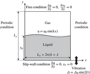
In the following, a 2D configuration is considered for simplicity. The main dynamics that is essential for the formation of a liquid ligament disintegrating into drops from a vertically vibrating liquid layer can be captured using a 2D simulation (Li & Umemura Reference Li and Umemura2014). The differences and similarities between 2D and three-dimensional (3D) configurations will be briefly discussed in § 4.1.5, as part of a discussion of the 2D calculation results. Figure 1 shows the 2D cell model used here, in which the effects of the container walls are excluded by imposing periodic boundary conditions at the horizontal boundaries. Definitions of the physical quantities in figure 1 will be described later. Details of the boundary conditions, as well as the geometry of the cell model, will be discussed in § 3.
Calculation domain of the cell model and boundary conditions.

2.3. Numerical strategy
The numerical strategy used to determine the threshold condition for spray formation is based on 2D Faraday instability theory under the assumptions described in § 1. When the surface deformation is small, the amplitude
 ${\it\delta}$
of the excited surface wave,
 ${\it\delta}(t)\sin (kx)$
, in the cell model obeys the Mathieu equation (Benjamin & Ursell Reference Benjamin and Ursell1954), i.e.
 $$\begin{eqnarray}\frac{\text{d}^{2}{\it\delta}}{\text{d}{\it\tau}^{2}}=\left(X\sin {\it\tau}-Y\right){\it\delta},\end{eqnarray}$$
where
 ${\it\tau}={\it\Omega}t$
. Let
 ${\it\omega}$
be the angular frequency of the free surface wave defined by
 ${\it\omega}^{2}={\it\sigma}k^{3}\tanh (ky_{0})/{\it\rho}_{l}$
. Whether or not the surface wave is stable is determined by two parameters,
 $X$
and
 $Y$
, which are defined as follows:
 $$\begin{eqnarray}X=k{\it\Delta}_{0}\tanh (ky_{0})\quad \text{and}\quad Y=\left(\frac{{\it\omega}}{{\it\Omega}}\right)^{2}=\frac{{\it\sigma}k^{3}\tanh (ky_{0})}{{\it\rho}_{l}{\it\Omega}^{2}}.\end{eqnarray}$$
Here, we consider the case whereby
 $\tanh (ky_{0})\rightarrow 1$
to eliminate the effects of liquid depth
 $y_{0}$
. Each surface wave specified by a parameter pair
 $(X,Y)$
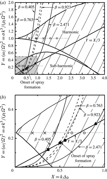
lying in the unstable regions shown in figure 2 increases its amplitude, and eventually reaches a standing-wave state or breakup state when the nonlinear effects prevail. According to the definitions of
 $X$
and
 $Y$
, the realisation for an experimental condition
 $({\it\Delta}_{0},{\it\Omega})$
can be expressed as a cubic curve
 $$\begin{eqnarray}Y=\frac{X^{3}}{{\it\beta}}\end{eqnarray}$$
in figure 2, by eliminating
 $k$
from (2.4). Equation (2.5) demonstrates that the possible linear surface waves that emerge in the experiment can be characterised by a dimensionless parameter
 ${\it\beta}=({\it\rho}_{l}{\it\Delta}_{0}^{3}{\it\Omega}^{2})/{\it\sigma}$
that is associated with the experimental forcing condition
 $({\it\Delta}_{0},{\it\Omega})$
. For this reason,
 ${\it\beta}$
is termed the dimensionless forcing strength hereafter. The wavenumbers that are excitable at a given value of
 ${\it\beta}$
are located on the cubic curve expressed by (2.5) in the unstable regions.
Unstable regions of the Mathieu equation (shown by the hatched areas) and illustration of the numerical strategy used to determine the threshold condition for spray formation. Panel (b) is an enlargement of the shadowed square region in (a). Each cubic curve represents one experimental condition characterised by the dimensionless forcing strength
 ${\it\beta}=({\it\rho}_{l}{\it\Delta}_{0}^{3}{\it\Omega}^{2})/{\it\sigma}$
. The points on the solid straight line
 $Y=X/3$
correspond to the predominant surface-wave modes at different values of
 ${\it\beta}$
. The filled square shows the non-atomisation case discussed in § 4.1.1. The filled triangle shows the atomisation case discussed in § 4.1.2. The filled diamond and circle show the near-critical cases discussed in § 4.1.3. The filled diamond represents the onset of spray formation. Cases other than those on the straight line
 $Y=X/3$
, represented by the cross symbols and open circles, are also simulated by fixing
 $Y=0.25$
and 1 and changing the value of
 $X$
. The cross symbols show cases for which breakup does not occur and the open circles show cases for which breakup does occur.

The results of ultrasonic atomisation experiments imply that, as discussed above, for each dimensionless forcing strength
 ${\it\beta}$
, we only need to calculate one case corresponding to the predominant surface wavenumber
 $k_{m}$
to determine whether a spray is formed if
 $k_{m}$
can be determined rationally. We describe an approach to determine
 $k_{m}$
in the following.
According to (2.3), when
 $$\begin{eqnarray}{\it\alpha}^{2}=X\sin {\it\tau}-Y=k{\it\Delta}_{0}\sin {\it\tau}-\frac{{\it\sigma}k^{3}}{{\it\rho}_{l}{\it\Omega}^{2}}>0,\end{eqnarray}$$
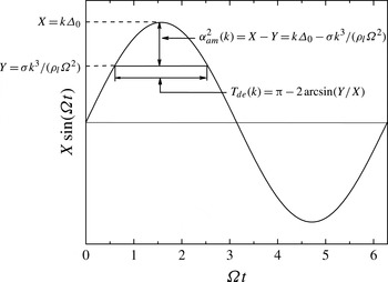
the amplitude of the surface wave in the unstable region tends to diverge during each oscillation cycle of the surface wave. If the amplified surface wave reaches a nonlinear stage during this period, the subsequent surface deformation no longer obeys the Mathieu equation. Therefore, the magnitude of (2.6) provides an indicator describing how fast the linear surface-wave evolution undergoes a transition into a nonlinear evolution, such as the formation of a steady standing wave or a liquid ligament dynamically free from the motion of the bulk liquid layer. The period over which
 ${\it\alpha}^{2}>0$
is referred to as the destabilising phase, with
 ${\it\alpha}>0$
indicating the growth rate. When
 ${\it\alpha}^{2}<0$
, the surface wave is in the stabilising phase. It should be noted that the magnitude of the growth rate is dependent on the wavenumber
 $k$
and dimensionless time
 ${\it\tau}$
for a given experimental condition
 $({\it\Delta}_{0},{\it\Omega})$
and properties of the liquid. The duration of the destabilising phase is given by
 $T_{de}(k)={\rm\pi}-2\arcsin [{\it\sigma}k^{2}/({\it\rho}_{l}{\it\Delta}_{0}{\it\Omega}^{2})]$
and the amplitude of the squared growth rate is
 ${\it\alpha}_{am}^{2}(k)=k{\it\Delta}_{0}-{\it\sigma}k^{3}/({\it\rho}_{l}{\it\Omega}^{2})$
(see figure 3). These are the two factors that influence the growth of the amplitude of the surface wave. Here,
 $T_{de}(k)$
is a decreasing function of
 $k$
, whereas
 ${\it\alpha}_{am}^{2}(k)$
assumes its peak value at
 $k=k_{m}$
. For a sufficiently large forcing strength, even though
 ${\it\alpha}_{am}(k)$
is small for other wavenumbers
 $k\neq k_{m}$
, the amplitude of the surface wave may become sufficiently large to form a liquid ligament and subsequent breakup after a long time has elapsed. However, we intend to find the minimum forcing strength under which spray formation can be initiated. It is clear that a liquid ligament disintegrating into drops begins to be formed in the destabilising phase. Therefore, we are interested in the surface wavenumber
 $k_{m}$
that maximises
 ${\it\alpha}_{am}$
for each forcing strength. The wavenumber
 $k_{m}$
that satisfies this condition is given by
 $$\begin{eqnarray}k_{m}^{2}=\frac{1}{3}\frac{{\it\rho}_{l}{\it\Delta}_{0}{\it\Omega}^{2}}{{\it\sigma}}.\end{eqnarray}$$
The surface waves with wavenumbers that satisfy (2.7) have the largest growth rate. For such surface waves, we have
 $$\begin{eqnarray}\left(\frac{{\it\omega}_{m}}{{\it\Omega}}\right)^{2}=\frac{1}{3}k_{m}{\it\Delta}_{0},\quad \text{namely},\quad Y_{m}=\frac{1}{3}X_{m}.\end{eqnarray}$$
Each point on the straight line
 $Y=X/3$
shown in figure 2 corresponds to the predominant surface-wave mode for a given dimensionless forcing strength
 ${\it\beta}$
. The problem is then reduced to determining the threshold dimensionless forcing strength
 ${\it\beta}_{c}$
for spray formation by simulating cases in which the wavelengths of the cell model are specified by the points
 $(X,Y)$
on the line
 $Y=X/3$
in the unstable regions.
Illustration of the duration of the destabilising phase,
 $T_{de}$
, and the amplitude of the squared growth rate,
 ${\it\alpha}_{am}^{2}$
.

3. Numerical methods
The numerical methods are based on those described in our previous study of the fundamental dynamics of ligament formation due to the Faraday instability (Li & Umemura Reference Li and Umemura2014), and have been validated via a comparison with other 2D numerical studies (Wright, Yon & Pozrikidis Reference Wright, Yon and Pozrikidis2000). All numerical calculations were carried out based on a frame of reference that moves with the sinusoidal motion of the substrate.
The 2D governing equations for the inviscid and incompressible liquid and gas flows are as follows:
 $$\begin{eqnarray}\left.\begin{array}{@{}c@{}}\boldsymbol{{\rm\nabla}}\boldsymbol{\cdot }\boldsymbol{u}_{\boldsymbol{r}}=0\\ \displaystyle {\it\rho}({\it\phi})\left[\frac{\partial \boldsymbol{u}_{\boldsymbol{r}}}{\partial t}+(\boldsymbol{u}_{\boldsymbol{r}}\boldsymbol{\cdot }\boldsymbol{{\rm\nabla}})\boldsymbol{u}_{\boldsymbol{r}}\right]=-\boldsymbol{{\rm\nabla}}p+{\it\rho}({\it\phi}){\it\Delta}_{0}{\it\Omega}^{2}\sin ({\it\Omega}t)\boldsymbol{j}+\boldsymbol{F}_{\boldsymbol{s}}\end{array}\right\},\end{eqnarray}$$
where
 $\boldsymbol{u}_{\boldsymbol{r}}=(u,v_{r})$
is the velocity vector; the vertical component
 $v_{r}$
corresponds to the vertical velocity referring to the vibrating bottom substrate;
 ${\it\rho}({\it\phi})={\it\rho}_{l}\cdot \text{H}_{{\it\varepsilon}}({\it\phi})+{\it\rho}_{g}\cdot [1-\text{H}_{{\it\varepsilon}}({\it\phi})]$
is the density function of the level-set (LS) function
 ${\it\phi}$
;
 $\text{H}_{{\it\varepsilon}}({\it\phi})$
is the smoothed Heaviside step function with a transition region of a constant thickness
 ${\it\varepsilon}$
;
 $p$
is pressure;
 $\boldsymbol{j}$
is the unit upward vector. The liquid-to-gas density ratio is
 ${\it\rho}_{l}/{\it\rho}_{g}=\ 50$
. This density ratio is considerably smaller than that commonly used for a water–air system, i.e.
 ${\it\rho}_{l}/{\it\rho}_{g}=850$
; however, it is the Atwood number
 $\text{A}_{t}=({\it\rho}_{l}-{\it\rho}_{g})/({\it\rho}_{l}+{\it\rho}_{g})$
that is used to evaluate the effects of the density ratio in Faraday instability problems. The Atwood numbers for the two cases are 0.96 and 0.99, which are both close to unity. As mentioned above, excellent agreement was found between our calculated results using
 $\text{A}_{t}=0.96$
(Li & Umemura Reference Li and Umemura2014) and those using
 $\text{A}_{t}=1$
(Wright et al.
Reference Wright, Yon and Pozrikidis2000), which indicates that the evolution of the surface deformation is not sensible with Atwood numbers in the range
 $0.96<\text{A}_{t}<1$
. Thus, the dynamics obtained in this work with
 ${\it\rho}_{l}/{\it\rho}_{g}=50$
describes the behaviour of a water–air system. Using the continuum surface force (CSF) method (Brackbill, Kothe & Zemach Reference Brackbill, Kothe and Zemach1992), surface tension is incorporated into the momentum equation (3.1) as a body force
 $\boldsymbol{F}_{\boldsymbol{s}}$
acting on an interfacial transition region of a constant thickness
 ${\it\varepsilon}$
,
 $$\begin{eqnarray}\boldsymbol{F}_{\boldsymbol{s}}={\it\sigma}{\it\kappa}\boldsymbol{{\rm\nabla}}\text{H}_{{\it\varepsilon}}({\it\phi}),\end{eqnarray}$$
where
 ${\it\kappa}=-\boldsymbol{{\rm\nabla}}\boldsymbol{\cdot }\boldsymbol{n}=-\boldsymbol{{\rm\nabla}}\boldsymbol{\cdot }(\boldsymbol{{\rm\nabla}}{\it\phi}/|\boldsymbol{{\rm\nabla}}{\it\phi}|)$
is the curvature of the liquid–gas interface and
 $\boldsymbol{n}$
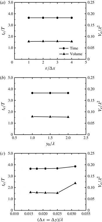
is the unit vector normal to that interface. As shown in figure 4(a), the thickness of the interfacial transition region in the range
 ${\rm\Delta}x<{\it\varepsilon}<4{\rm\Delta}x$
, where
 ${\rm\Delta}x(={\it\lambda}/64)$
is the horizontal grid size, does not significantly affect the time for ejection of the first drop
 $t_{e}$
or the volume
 $V_{e}$
of that drop for an atomisation case
 $(X=0.9075,Y=0.3025)$
discussed in § 4.1.2. We used
 ${\it\varepsilon}=3{\rm\Delta}x$
for all calculations.
Dependence of the time for ejection of the first drop
 $t_{e}$
and the volume
 $V_{e}$
of that drop as a function of (a) the thickness
 ${\it\varepsilon}$
of the interfacial transition region, (b) the liquid depth
 $y_{0}$
and (c) the grid resolution
 ${\rm\Delta}x={\rm\Delta}y$
. It should be noted that (a) and (b) correspond to a grid resolution of
 ${\rm\Delta}x={\rm\Delta}y={\it\lambda}/64$
. Here,
 $T=1/f=2{\rm\pi}/{\it\Omega}$
is the forcing period.

Equations (3.1) were solved for the cell model with the boundary conditions described in figure 1. In the horizontal direction, periodic boundary conditions were imposed at the left- and right-hand side boundaries. With the CSF method, it is not necessary to impose boundary conditions on the liquid–gas interface. A free boundary was imposed at the top of the calculation domain. In the Faraday instability problem, the major dynamics of interest occurs over a range of depths that extends approximately
 $1/k$
from the liquid–gas interface. It is therefore unnecessary, as well as extremely time-consuming, to simulate liquid layers with depths much larger than
 $1/k$
. The liquid deeper than
 $1/k$
merely moves essentially with the vibrating substrate, and thus the details of this motion can be neglected (Li & Umemura Reference Li and Umemura2014). We then set the liquid depth
 $y_{0}={\it\lambda}=2{\rm\pi}/k$
, which makes the simulation realisable. We also set the bottom boundary of the cell model as a slip wall. The calculation domain spanned one wavelength horizontally
 $(L_{x}={\it\lambda})$
and two and a half wavelengths vertically
 $(L_{y}=2.5{\it\lambda})$
. We carried out two other calculations with different liquid depths, i.e.
 $y_{0}=1.5{\it\lambda}\ (L_{y}=3.0{\it\lambda})$
, and
 $y_{0}=2.0{\it\lambda}\ (L_{y}=3.5{\it\lambda})$
for the atomisation case
 $(X=0.9075,Y=0.3025)$
. Figure 4(b) shows that the dynamics is independent of the liquid depth
 $y_{0}$
when
 $y_{0}>{\it\lambda}$
.
With the cell model, we must introduce an initial surface disturbance
 ${\it\eta}(t=0,x)$
, which can be decomposed as a Fourier series
 $\sum _{k}{\it\eta}_{k}(t=0)\sin (kx)$
. The disturbance
 ${\it\eta}$
can be any surface displacement or surface vertical velocity; however, because we are interested in identifying the predominant surface wave, only a sinusoidal surface disturbance was imposed as an initial surface condition. Two limiting conditions for the initial surface can be considered, which are described as follows.
-
(a) A small initial surface disturbance, for which the surface deformation obeys the Mathieu equation during the early stages of development. When the system is unstable, the surface deformation is amplified; however, the system finally settles into a steady state determined by the forcing strength. This case will be treated in § 4.1.
-
(b) A large initial surface disturbance, for which the initially introduced excess energy is removed from the liquid layer via the formation of drops. The system eventually settles down to a steady state, which is determined by the forcing strength. This case will be treated in § 4.2.
The numerical results in § 4.2 show that, regardless of which initial condition is imposed, the same steady state will eventually be reached for a given forcing strength. The threshold forcing strength for spray formation is not dependent on the initial conditions of the surface. It is more convenient to use a small surface disturbance for the initial condition to determine the threshold condition in the numerical studies. In this work, unless otherwise stated, the initial surface disturbance was introduced into the cell model as a vertical surface deformation velocity distribution
 $v_{s}=v_{s0}\sin (kx)$
, where
 $v_{s0}=0.03{\it\Delta}_{0}{\it\Omega}$
. In the frame of reference moving with the vibrating bottom substrate, the initial velocity was zero, except at the liquid surface. The initial surface was flat, and the pressure was hydrostatic.
The governing equations were discretised on a uniform staggered grid. The grid resolution effects were evaluated by comparing the numerical results of the atomisation case
 $(X=0.9075,Y=0.3025)$
for different grid resolutions (
 ${\rm\Delta}x={\rm\Delta}y={\it\lambda}/32$
,
 ${\it\lambda}/40$
,
 ${\it\lambda}/48$
,
 ${\it\lambda}/56$
and
 ${\it\lambda}/64$
), which are shown in figure 4(c). For a grid resolution finer than
 ${\it\lambda}/32$
, any further decrease in the grid size had little effect on the time for ejection of the first drop
 $t_{e}$
or the volume
 $V_{e}$
of that drop. The grid resolution in this work was set to
 ${\rm\Delta}x={\rm\Delta}y={\it\lambda}/64$
.
The marker-and-cell (MAC) method (Harlow & Welch Reference Harlow and Welch1965) was used to calculate the pressure and velocity fields. In this projection method, the intermediate velocity field was first advanced using a second-order upwind scheme to discretise the convective terms. The divergence of this intermediate velocity was then used as the source term for the pressure Poisson equation, which was solved iteratively using the successive over-relaxation (SOR) method. The convergence criterion was set to a residual of
 $10^{-10}$
. The resulting pressure was used to update the velocity field at the next instant. The time step
 ${\rm\Delta}t$
was adjusted for each calculation cycle to ensure numerical stability. Two restrictions were imposed on the time step for each iteration: the material points and capillary waves could not move more than one grid size in one time step (Nichols, Hirt & Hotchkiss Reference Nichols, Hirt and Hotchkiss1980), i.e.
 $$\begin{eqnarray}{\rm\Delta}t=\min \left[C\frac{{\rm\Delta}x}{|U|},C\frac{{\rm\Delta}y}{|V|},\sqrt{\frac{\min ({\it\rho}_{l},{\it\rho}_{g})\cdot \min ({\rm\Delta}x,{\rm\Delta}y)^{3}}{4{\it\sigma}}}\right],\end{eqnarray}$$
where
 $U$
and
 $V$
are the maximum magnitudes of the horizontal and vertical velocities in the entire calculation domain at each instant, respectively, and
 $C=0.25$
is the Courant number. The largest time step in the calculations was
 ${\sim}0.005T\ll T$
, where
 $T=1/f=2{\rm\pi}/{\it\Omega}$
is the forcing period. This indicates that at least two hundred time steps were simulated in each forcing period.
The liquid–gas interface was tracked implicitly via the LS function
 ${\it\phi}$
, which is the signed normal distance from the interface (
 ${\it\phi}>0$
in the liquid and
 ${\it\phi}<0$
in the gas). However, the LS method does not conserve volume during the reinitialisation process, which is required to maintain
 ${\it\phi}$
as the signed normal distance function. For this reason, we used the volume-of-fluid (VOF) method to conserve volume. Such an approach is commonly referred to as the coupled level-set and volume-of-fluid (CLSVOF) method. In this work, we used the mass-conserving level-set (MCLS) method (Van der Pijl et al.
Reference Van der Pijl, Segal, Vuik and Wesseling2005), whereby the volume change was less than 1 %, even in atomisation cases.
To investigate the accuracy of the curvature and surface tension forces evaluated using the CLSVOF/CSF method, we compared the pressure of a static drop of radius
 $R$
calculated using our method,
 $p_{c}$
, with the theoretical value,
 $p_{t}$
, for grid resolutions of
 $R/{\rm\Delta}x=4$
, 8, 16 and 32. The errors between these two pressures were
 $|p_{c}-p_{t}|/p_{t}=0.049$
, 0.011, 0.0025 and 0.00075, respectively, for the four different grid sizes. These errors in pressure were smaller than those obtained by Brackbill et al. (Reference Brackbill, Kothe and Zemach1992), who used the VOF/CSF method only.
4. Results and discussion
4.1. Numerically determined threshold condition for spray formation
When carrying out calculations using the cell model, it is convenient to normalise the coordinates (
 $x,y$
) by the cell width
 ${\it\lambda}=2{\rm\pi}/k$
and the time
 $t$
by the forcing angular frequency
 ${\it\Omega}$
such that
 $(\tilde{x},{\tilde{y}})=(x,y)/{\it\lambda}$
and
 $\tilde{t}={\it\Omega}t$
. Because the velocity field produced by the inertial force
 ${\it\rho}{\it\Delta}_{0}{\it\Omega}^{2}\sin ({\it\Omega}t)$
must depend on the forcing displacement amplitude
 ${\it\Delta}_{0}$
as well, we used the following dimensionless velocity and pressure fields:
 $\tilde{\boldsymbol{u}}_{\boldsymbol{r}}=\boldsymbol{u}_{\boldsymbol{r}}/({\it\Delta}_{0}{\it\Omega})$
and
 $\tilde{p}=p/({\it\rho}{\it\Delta}_{0}{\it\Omega}^{2}{\it\lambda})$
. Equations (3.1) can then be rewritten as follows:
 $$\begin{eqnarray}\left.\begin{array}{@{}c@{}}\tilde{\boldsymbol{{\rm\nabla}}}\boldsymbol{\cdot }\tilde{\boldsymbol{u}}_{\boldsymbol{r}}=0\\ \displaystyle \frac{\partial \tilde{\boldsymbol{u}}_{\boldsymbol{r}}}{\partial \tilde{t}}+\frac{X}{2{\rm\pi}}(\tilde{\boldsymbol{u}}_{\boldsymbol{r}}\boldsymbol{\cdot }\tilde{\boldsymbol{{\rm\nabla}}})\tilde{\boldsymbol{u}}_{\boldsymbol{r}}=-\tilde{\boldsymbol{{\rm\nabla}}}\tilde{p}+\sin (\tilde{t})\boldsymbol{j}-\frac{Y}{(2{\rm\pi})^{2}X}\tilde{\boldsymbol{{\rm\nabla}}}\boldsymbol{\cdot }\boldsymbol{n}\tilde{\boldsymbol{{\rm\nabla}}}\text{H}\end{array}\right\},\end{eqnarray}$$
where the parameters
 $X$
and
 $Y$
are defined in (2.4). The boundary conditions do not contain any parameters.
Given the experimental conditions (
 ${\it\Delta}_{0},{\it\Omega}$
), which are the only controllable variables for a given infinitely extended deep liquid layer, the value of the dimensionless forcing strength
 ${\it\beta}$
is determined from
 ${\it\beta}=({\it\rho}_{l}{\it\Delta}_{0}^{3}{\it\Omega}^{2})/{\it\sigma}$
. We consider a series of experiments starting with a small
 ${\it\beta}$
and examine how the surface deformation feature changes with
 ${\it\beta}$
. According to the selection concept, the fastest growing disturbance mode will prevail with each experimental condition. Therefore, according to the numerical strategy described in § 2, we calculate the evolution of a linear wave mode on the line
 $Y=X/3$
(see figure 2) for each experimental condition characterised by
 ${\it\beta}$
. In this case, the parameters
 $X$
and
 $Y$
in (4.1) take the values
 $X=\sqrt{{\it\beta}/3}$
and
 $Y=\sqrt{{\it\beta}/3^{3}}$
. Therefore, (4.1) can be rewritten as follows:
 $$\begin{eqnarray}\left.\begin{array}{@{}c@{}}\tilde{\boldsymbol{{\rm\nabla}}}\boldsymbol{\cdot }\tilde{\boldsymbol{u}}_{\boldsymbol{r}}=0\\ \displaystyle \frac{\partial \tilde{\boldsymbol{u}}_{\boldsymbol{r}}}{\partial \tilde{t}}+\frac{\sqrt{{\it\beta}}}{2\sqrt{3}{\rm\pi}}(\tilde{\boldsymbol{u}}_{\boldsymbol{r}}\boldsymbol{\cdot }\tilde{\boldsymbol{{\rm\nabla}}})\tilde{\boldsymbol{u}}_{\boldsymbol{r}}=-\tilde{\boldsymbol{{\rm\nabla}}}\tilde{p}+\sin (\tilde{t})\boldsymbol{j}-\frac{1}{(2\sqrt{3}{\rm\pi})^{2}}\tilde{\boldsymbol{{\rm\nabla}}}\boldsymbol{\cdot }\boldsymbol{n}\tilde{\boldsymbol{{\rm\nabla}}}\text{H}\end{array}\right\}.\end{eqnarray}$$
This indicates that the surface deformation feature with each experimental condition is determined by
 ${\it\beta}$
only. With a small value of
 ${\it\beta}$
, the above equations describe the evolution of a linear wave. For relatively large values of
 ${\it\beta}$
, all terms become comparable in the liquid phase, and the convective term contributes to the surface deformation. It should be noted that the dimensionless equations (4.2) do not account for a flow structure whereby the surface deformation is confined to a thin layer at the interface. Therefore, the condition
 ${\it\beta}\sim 12{\rm\pi}^{2}\sim 100$
, derived by simply equating
 $\sqrt{{\it\beta}}/(2\sqrt{3}{\rm\pi})$
to unity in (4.2), does not express the balance between the unsteady and convective terms in the calculated flow.
Six cases were simulated, i.e.
 $(X=0.3675,Y=0.1225)$
,
 $(X=0.4564,Y=0.1521)$
,
 $(X=0.5043,Y=0.1681)$
,
 $(X=0.5547,Y=0.1849)$
,
 $(X=0.6075,Y=0.2025)$
and
 $(X=0.9075,Y=0.3025)$
, corresponding to the dimensionless forcing strengths
 ${\it\beta}=0.405$
, 0.625, 0.763, 0.923, 1.107 and 2.471, respectively, to determine the threshold condition for spray formation. One should consider that the threshold condition for spray formation from the entire liquid layer is equivalent to that for repeated drop formation in the cell model of the predominant surface wavelength. A disintegrating liquid ligament may form in a destabilising phase, even with a relatively small forcing strength, as long as sufficient time elapses. However, the broken drop will not have an outward velocity in the laboratory reference frame, and will fall back and coalesce with the liquid layer. Therefore, a spray is not formed under such conditions. A further increase in the forcing strength increases the vertical velocity of the broken drop. Since viscous and gravitational effects are neglected, whether or not the broken drop leaves the liquid layer depends only on its centre-of-mass velocity at the instant when breakup occurs. Therefore, the criterion for spray formation used here is that the drop holds a zero area-averaged vertical velocity in the laboratory reference frame
 $(v_{d}=0)$
at the instant of breakup. With this criterion, the calculation results show that the threshold dimensionless forcing strength for spray formation is around
 ${\it\beta}_{c}=0.763\sim O(1)$
.
In addition to the calculation cases of predominant surface wavelengths, we calculated other cases that are not located on the line
 $Y=X/3$
. The results show that drops only depart from the liquid layer in the cases to the right of the cubic curve
 $Y=X^{3}/{\it\beta}_{c}$
, which validates the threshold condition described above.
In the following, we explain the calculation results. We describe the dynamic change in the Faraday instability as a function of
 ${\it\beta}$
, and then identify the threshold value of
 ${\it\beta}$
.
4.1.1. Non-atomisation case
Figure 5(a) shows the temporal evolution of the surface displacement at
 $x={\it\lambda}/4$
for the case
 $(X=0.3675,Y=0.1225)$
(filled square in figure 2,
 ${\it\beta}=0.405$
). The corresponding solution of the Mathieu equation (2.3), calculated with a fourth-order Runge–Kutta method, is also shown by the dashed line in figure 5(a). Although the parameter pair
 $(X=0.3675,Y=0.1225)$
lies in the unstable region, atomisation does not occur. The amplitude of the surface displacement eventually reaches a steady-state value of approximately
 $0.17{\it\lambda}$
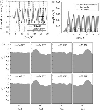
. This may be considered to be the realisation of a Faraday standing wave. In the early stages of the simulation, when the surface displacement is small, the calculation results agree well with the linear solution. Some deviation between the calculation results and the linear solution arises when higher-order modes of the surface deformation become more significant, as shown in figure 5(b), in which the temporal evolutions of the three lowest-order spatial modes obtained from a Fourier decomposition of the surface deformation are shown. In the standing-wave state, the amplitude of the surface displacement varies slightly from one period to the next, tending to become saturated rather than amplified. Figure 5(c) shows the shape of the surface at the times shown by the filled circles in figure 5(a) over two periods of the surface deformation cycles. When the Faraday standing wave occurs, the same surface deformation is repeated in subsequent cycles.
Calculation results for the case
 $(X=0.3675,Y=0.1225)$
(filled square in figure 2,
 ${\it\beta}=0.405$
), where a Faraday standing wave forms. (a) Temporal evolution of the surface displacement at
 $x={\it\lambda}/4$
(solid line). The dashed line shows the solution of the Mathieu equation with the same parameters and initial conditions as the numerical calculation. (b) Temporal evolution of the three lowest-order spatial modes. (c) Comparison between the surface shapes at the times shown by the filled circles in (a) in two different cycles.

Work done on the liquid layer by the inertial force for the case
 $(X=0.3675,Y=0.1225)$
. (a) Temporal evolution of the work rate. (b) Data plotted in (a) over the range
 $20.3T<t<22.3T$
, along with the temporal evolutions of the surface displacement at
 $x={\it\lambda}/4$
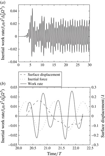
and the inertial force.

We have assumed that the flow is inviscid. Therefore, the standing wave corresponds to zero net work done on the liquid layer by the inertial force during one period of the surface deformation cycle. Figure 6(a) shows the temporal evolution of the work rate (per unit length in the
 $z$
direction) performed by the inertial force on the liquid layer region, i.e.
 ${\it\rho}_{l}\iint {\it\Delta}_{0}{\it\Omega}^{2}\sin ({\it\Omega}t)\cdot v_{r}\text{d}x\text{d}y$
. During the early stages of the simulation, the work rate is mostly positive because the liquid layer flow resonates with the inertial force oscillations (linear instability). As a result, the amplitude of the surface displacement grows rapidly with time. When the surface deformation becomes relatively large, nonlinear effects prevail, which delays the recovery of the surface crest or trough to the neutral position because the liquid flowing at a large velocity tends to maintain the same velocity due to the inertia. As such, a phase difference is created between the liquid layer flow and the inertial force. This phase difference is shown in figure 6(b), in which the temporal evolutions of the surface displacement at
 $x={\it\lambda}/4$
and the inertial work rate are shown for one period of the surface deformation cycle in the standing-wave state. This phase difference increases the negative work rate, and thereby decreases the growth rate of the surface displacement amplitude. During the interval
 $20.5T<t<21T$
, the inertial force is negative, and the following behaviour is observed. First, the liquid flows towards the crest. Because most of the liquid moves upwards, the work rate, which is the product of the inertial force and the vertical velocity, is negative. The liquid flow then changes direction after approximately
 $t=20.75T$
, resulting in a positive work rate. Similar behaviour occurs repeatedly, resulting in zero net work over one period of the surface deformation cycle.
Temporal evolution of the surface height at
 $x=3{\it\lambda}/4$
for the case (
 $X=0.9075$
,
 $Y=0.3025$
) (filled triangle in figure 2,
 ${\it\beta}=2.471$
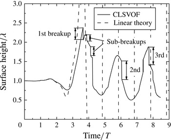
), in which breakup occurs continuously, as indicated by the discontinuities. The dashed line shows the solution of the Mathieu equation with the same parameters and initial conditions as the numerical calculation.

4.1.2. Atomisation case
Figure 7 shows the temporal evolution of the surface height at
 $x=3{\it\lambda}/4$
for the case
 $(X=0.9075,Y=0.3025)$
(filled triangle in figure 2,
 ${\it\beta}=2.471$
). In this case, due to the strong forcing, a free ligament forms and its first breakup occurs at a relatively early stage. When the surface deformation is small, the calculation results agree well with the solution of the Mathieu equation (shown by the dashed line in figure 7). When the surface deformation becomes large, although the phase is delayed compared with the linear solution, the surface deformation still oscillates with a period
 $2T$
, consistent with the experimental observations that drops are formed from the subharmonically oscillating liquid surface (Lang Reference Lang1962; Rajan & Pandit Reference Rajan and Pandit2001; Donnelly et al.
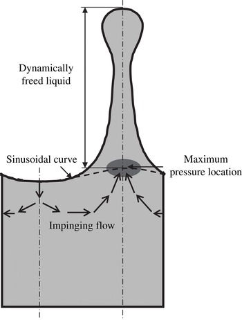
Reference Donnelly, Hogan, Mugler, Schommer, Schubmehl, Bernoff and Forrest2004). Because the period of the resulting unstable liquid layer flow is fixed by the forcing frequency, an increase in the forcing strength increases the magnitude of the liquid velocity. As a result, the convective term in the governing equations (3.1) becomes more effective. We have previously described the detailed dynamics of ligament formation due to the Faraday instability (Li & Umemura Reference Li and Umemura2014), as illustrated in figure 8. The impingement of the liquid flowing from the neighbouring trough portions increases the pressure at the crest root. If this pressure is larger than the capillary pressure, then the crest grows to form a slender ligament, in which the liquid pressure relaxes to the surrounding uniform gas pressure. Thus, increased pressure at the ligament (crest) root takes the form of a local maximum pressure location. This means that the liquid ligament above this location becomes dynamically free from the motion of the bulk liquid below this location. As a result, liquid flowing from the trough portions and passing the local maximum pressure location moves upwards freely and elongates the ligament. Thus, the resulting liquid ligament behaves like a low-speed water jet ejected vertically downwards from an orifice under gravity, and tends to disintegrate into drops (Stone & Leal Reference Stone and Leal1989a
,Reference Stone and Leal
b
; Schulkes Reference Schulkes1994; Umemura Reference Umemura2011; Umemura et al.
Reference Umemura, Kawanabe, Suzuki and Osaka2011).
Essential dynamics of liquid ligament formation due to the Faraday instability.

The breakup of a liquid ligament is indicated by an abrupt drop in the surface height, as shown in figure 7. The first breakup of a ligament, resulting in an outward moving drop, occurs at
 $t=3.65T$
, followed by two sub-breakups of the same ligament. The drops that result from these sub-breakups move towards the liquid layer and coalesce with it. If the forcing strength increases further, multiple drops with non-zero velocities in the direction away from the liquid layer could form from a ligament. After these breakups occur, the free ligament disappears in the following stabilising phase. Because the resulting relatively flattened surface is similar to the initial surface of the liquid layer, but with a finite amplitude, similar repeatable events occur, i.e. steady atomisation. Figure 7 shows that the second and third breakups occur over subsequent time periods.
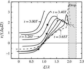
Figure 9 shows the vertical velocity distribution along the crest centreline (
 $x=3{\it\lambda}/4$
) for times
 $3.00T<t<3.65T$
, during which a long ligament forms. The abscissa
 ${\it\xi}$
is the distance measured from the middle position of the vibrating bottom substrate, while the ordinate
 $v$
is the vertical velocity normalised by
 ${\it\Delta}_{0}{\it\Omega}$
viewed in the laboratory reference frame. At
 $t=3.00T$
, the bottom substrate moves upwards from the middle position with a large velocity. The filled circles in figure 9 show the positions of the local maximum pressure location that appears at
 $t=3.20T$
, and then moves downwards abruptly. When a free ligament forms, a liquid element passing the local maximum pressure location with a vertical velocity
 $v$
at time
 $t_{0}$
moves upwards, maintaining the same momentum. Such dynamic features continue until the local maximum pressure location disappears in the following stabilising phase. Thus, the instantaneous velocity
 $v$
and the distance
 ${\it\xi}$
of the liquid element at a later time
 $t$
(before the local maximum pressure location disappears) can be described by the following equations:
 $$\begin{eqnarray}\left.\begin{array}{@{}l@{}}v(t)={\it\Delta}_{0}{\it\Omega}\cos ({\it\Omega}t_{0})+v_{r}(t_{0})\\ {\it\xi}={\it\Delta}_{0}\sin ({\it\Omega}t_{0})+h(t_{0})+v\cdot (t-t_{0})\end{array}\right\},\end{eqnarray}$$
where
 $v_{r}(t_{0})$
and
 $h(t_{0})$
are the vertical velocity and vertical distance of the liquid element referring to the vibrating bottom substrate at time
 $t_{0}$
, respectively. According to (4.3), a liquid element that holds
 $v=0$
in the free ligament region should be fixed in space (
 ${\it\xi}={\it\Delta}_{0}\sin ({\it\Omega}t_{0})+h(t_{0})$
), consistent with the data shown in figure 9 after
 $t=3.40T$
.
Vertical velocity distribution along the crest centreline (
 $x=3{\it\lambda}/4$
) during the interval
 $3.00T<t<3.65T$
for the case
 ${\it\beta}=2.471$
(Li & Umemura Reference Li and Umemura2014), courtesy of Elsevier. The velocity is viewed in the laboratory reference frame. The plots are drawn at temporal intervals of
 $0.10T$
. The dashed curve corresponds to the instant
 $t=3.65T$
when the first breakup occurs. The filled circles show the positions of the local maximum pressure location. The shadowed region represents the broken drop.

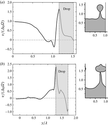
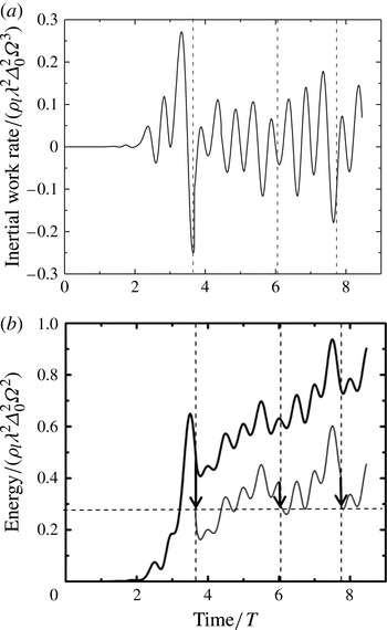
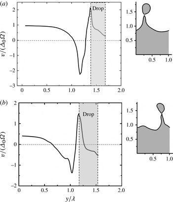
Figures 10(a,b) show the vertical velocity distributions along the crest centreline at the instants of the second and third breakups. The velocity is viewed in the laboratory reference frame. It is clear that the vertical velocities in the drop region are positive, except where the drop tip recedes due to the surface tension. The broken drops with positive area-averaged velocities rise away from the liquid layer. Therefore, once breakup occurs at the tip of a ligament, the liquid layer loses the mass and energy of the broken drop. This means that spray formation due to the Faraday instability is a process whereby the liquid layer absorbs energy from the inertial force, and then partially releases it by producing drops that leave the liquid layer. In particular, steady atomisation is realised when the energy gain becomes equal to the energy loss averaged over time. Figures 11(a,b) show the temporal evolutions of the inertial work rate (per unit length in the
 $z$
direction) and its time integration, i.e.
 ${\it\rho}_{l}\int _{0}^{t}(\iint {\it\Delta}_{0}{\it\Omega}^{2}\sin ({\it\Omega}t)\cdot v_{r}\text{d}x\text{d}y)\text{d}t$
. The energy absorbed by the liquid layer due to the work done by the inertial force between two breakups is utilised to release the next drop. This indicates that broken drops form repeatedly.
Vertical velocity distribution along the crest centreline (
 $x=3{\it\lambda}/4$
) for the case
 $(X=0.9075,Y=0.3025)$
at (a)
 $t=6.04T$
and (b)
 $t=7.74T$
, corresponding to the second and third breakups shown in figure 7, respectively. The velocity is viewed in the laboratory reference frame. The insets show the surface shape at the corresponding instants.

Work done on the liquid layer by the inertial force for the case
 $(X=0.9075,Y=0.3025)$
. (a) Temporal evolution of the inertial work rate. (b) Temporal evolutions of the inertial work (thick solid line) and the energy of the liquid layer (thin solid line), which is obtained by subtracting the surface and kinetic energies of the broken drops (shown by the downward arrows) from the inertial work. The three vertical dashed lines represent three breakup instants. The arrow tips indicate the energy of the liquid layer immediately following breakup, which is almost constant, as shown by the horizontal dashed line connecting the three arrow tips.

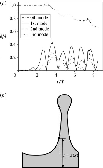
A Fourier decomposition of the surface deformation is conventionally used to gain insight into higher-order components of the waveform, and is indeed useful to analyse cases in which atomisation does not occur. However, we encounter some difficulties in doing so when atomisation occurs. Figure 12(a) shows the temporal evolutions of the three lowest-order spatial modes obtained by a Fourier decomposition of the surface deformation for the case
 $(X=0.9075,Y=0.3025)$
. The zeroth mode corresponds to the mean height of the liquid layer surface. In principle, this should decrease discontinuously by an amount corresponding to the volume of the broken drop that leaves the liquid layer. The Fourier decomposition ceases to be a good description of the system when a ligament with a bulbous tip is formed, as shown in figure 12(b). The surface profile,
 $s=s(x)$
, becomes a multivalued function. In the present Fourier decomposition of such a surface profile, the lowest point (shown by the filled circle in figure 12
b) is used as the surface point at this abscissa. Therefore, the mean height of the liquid layer surface decreases before breakup. It should be noted that the amplitudes of the second and third modes become almost comparable with that of the first (fundamental) mode once a ligament forms, but they are mainly the result of the protruding shape of the ligament used in the Fourier decomposition. As described above, a free ligament above the local maximum pressure location has no dynamic connection with the behaviour of the liquid layer below this location; thus, a simple Fourier decomposition of the surface deformation does not reflect the fundamental motion of the liquid layer. If we remove the free ligament (i.e. liquid region above the local maximum pressure location) from the liquid layer, the shape of the trough surface and the ‘new crest surface’ (the top of which is at the local maximum pressure location) can be approximated as a sinusoidal curve with the fundamental wavelength, as shown by the dashed curve in figure 8.
Fourier decomposition of the surface deformation in the case (
 $X=0.9075$
,
 $Y=0.3025$
). (a) Temporal evolutions of the three lowest-order spatial modes and the zeroth mode. (b) Multivalued surface profile function due to the bulbous tip.

4.1.3. Near-critical case
The threshold dimensionless forcing strength for spray formation should be between the two cases discussed in the previous two sections. In this section, we consider two further cases near the threshold condition.
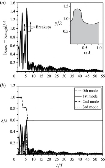
Figure 13 shows the temporal evolution of the distance between the crest top and the trough bottom,
 $|y_{crest}-y_{trough}|$
, for the case
 $(X=0.5547,Y=0.1849)$
(filled circle in figure 2,
 ${\it\beta}=0.923$
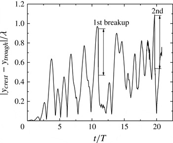
). We chose this distance rather than the surface displacement at a fixed horizontal position because, in this case, the crest moves in the horizontal direction after the first breakup occurs. Similarly to the atomisation case discussed in § 4.1.2, breakups take place in this near-critical case, but the breakup rate is one breakup over ten forcing periods, which is considerably less than what occurs in the atomisation case (one breakup over two forcing periods).
Temporal evolution of the distance between the crest top and the trough bottom,
 $|y_{crest}-y_{trough}|$
, for the case (
 $X=0.5547,Y=0.1849$
) (filled circle in figure 2,
 ${\it\beta}=0.923$
).

Figure 14(a) shows the vertical velocity distribution along the crest centreline at the instant the first breakup occurs. The velocity is viewed in the laboratory reference frame. The area-averaged vertical velocity of the drop is positive, implying that the broken drop moves outward from the liquid layer.
Vertical velocity distribution along the crest centreline at the instant the first breakup occurs for (a) (
 $X=0.5547,Y=0.1849$
) at
 $t=10.98T$
and (b) (
 $X=0.5043$
,
 $Y=0.1681$
) (filled diamond in figure 2,
 ${\it\beta}=0.763$
) at
 $t=10.75T$
. The velocity is viewed in the laboratory reference frame. The insets show the surface shape at the corresponding instants.

However, when the forcing strength is further reduced, negative vertical velocities emerge at the upper portion of the broken drop, as shown in figure 14(b), for the case (
 $X=0.5043,Y=0.1681$
) (filled diamond in figure 2,
 ${\it\beta}=0.763$
). This may reduce the area-averaged vertical velocity in the laboratory reference frame,
 $v_{d}$
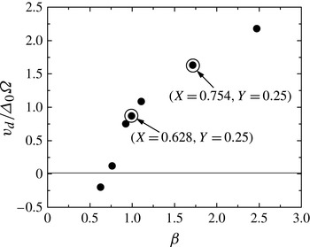
, with which the broken drop moves outward from the liquid layer. Figure 15 shows
 $v_{d}$
as a function of the dimensionless forcing strength
 ${\it\beta}$
. According to the criterion defined here, i.e.
 $v_{d}=0$
, the onset of spray formation occurs when the dimensionless forcing strength is approximately 0.763. We therefore arrive at a threshold dimensionless forcing strength for spray formation of
 ${\it\beta}_{c}=0.763$
.
Area-averaged vertical velocity of the broken drop at the instant of the first breakup,
 $v_{d}$
, as a function of
 ${\it\beta}$
. Here,
 $v_{d}$
is viewed in the laboratory reference frame.

Other cases that are not located on the straight line
 $Y=X/3$
were also calculated by fixing
 $Y=0.25$
and
 $Y=1.0$
and changing the value of
 $X$
, as indicated by the cross symbols (no breakup occurs) and the open circles (breakup occurs) in figure 2. The results show that atomisation occurs to the right of the dashed curve (
 $Y=X^{3}/{\it\beta}_{c}$
), which validates the numerical strategy used in this work.
4.1.4. Theoretical consideration
Based on the cell model which embodies the conventional selection concept and the physics underlying the well-known Landau amplitude equation (Müller Reference Müller1994; Chen & Viñals Reference Chen and Viñals1999; Aranson & Kramer Reference Aranson and Kramer2002), our numerical calculations starting from a small initial surface disturbance have identified the threshold dimensionless forcing strength for spray formation as
 ${\it\beta}_{c}=0.763$
. The validity of this numerical result can be supported from the following simple theoretical considerations.
As described in § 4.1.2, once a free ligament forms, it may naturally disintegrate into drops. Therefore, the threshold condition primarily corresponds to the free ligament formation condition, and crucially relies on the velocity enhancement of the horizontal flow oscillating at half the forcing frequency,
 ${\it\Omega}/2$
. The momentum equation for the horizontal velocity component
 $u$
in (3.1) indicates that the order of magnitude of the maximum horizontal velocity attainable at the mid-location between the crest and trough portions in a cycle,
 $u_{max}$
, when the convective term becomes comparable in magnitude to the unsteady term, can be estimated as
 $u_{max}\sim {\it\lambda}{\it\Omega}/(2{\rm\pi})$
because the unsteady term and the convective term may be estimated as
 $(u_{max}-0)/(2{\rm\pi}/({\it\Omega}/2)/4)=u_{max}{\it\Omega}/{\rm\pi}$
and
 $(u_{max}/2)(u_{max}-0)/({\it\lambda}/4)=2u_{max}^{2}/{\it\lambda}$
, respectively. The order of magnitude of the vertical velocity
 $v_{rmax}$
(referring to the vibrating bottom substrate) due to the impingement of this horizontal flow of a depth of
 $1/k$
can be estimated as
 $v_{rmax}\sim {\it\lambda}{\it\Omega}/{\rm\pi}^{2}$
by using the continuity relation,
 $(1/k)u_{max}\sim ({\it\lambda}/4)v_{rmax}$
. Therefore, we arrive at the following expression:
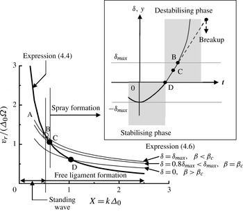
 $$\begin{eqnarray}\frac{v_{rmax}}{{\it\Delta}_{0}{\it\Omega}}\sim \frac{{\it\lambda}}{{\rm\pi}^{2}{\it\Delta}_{0}}=\frac{2}{{\rm\pi}k{\it\Delta}_{0}}=\frac{2}{{\rm\pi}}\frac{1}{X}.\end{eqnarray}$$
As shown in figure 2,
 $X\sim 0.9$
for the atomisation case with
 ${\it\beta}=2.471$
. Therefore, (4.4) leads to
 $v_{rmax}/({\it\Delta}_{0}{\it\Omega})\sim 0.71\sim O(1)$
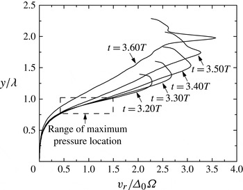
, which is consistent with the results of the numerical calculations shown in figure 16. It should be noted that in atomisation cases, a liquid ligament above the maximum pressure location is dynamically free from the bulk liquid region below that location. According to Li & Umemura (Reference Li and Umemura2014), the ligament-producing liquid velocity should be the vertical velocity
 $v_{rmax}$
at the maximum pressure location (the range of the maximum pressure location at different instants is shown by the dashed rectangle in figure 16), which is a direct result of the impingement of the horizontal flow satisfying the abovementioned continuity relation. As
 ${\it\beta}$
approaches zero, the value of
 $v_{rmax}$
in (4.4) increases divergently. However, at small
 $X$
, and thereby small
 ${\it\beta}$
, the Faraday instability cannot induce a horizontal flow satisfying (4.4). Equation (4.4) is valid for
 $X$
greater than some particular value, which may be estimated as follows.
Vertical velocity distribution along the crest centreline (
 $x=3{\it\lambda}/4$
) for the atomisation case
 ${\it\beta}=2.471$
, from the time the maximum pressure location emerges (
 $t=3.20T$
) to when the first breakup is about to occur (
 $t=3.60T$
). The velocity refers to the vibrating bottom substrate. The range of the maximum pressure location is shown by the dashed rectangle.

An important finding of both the work reported here and that of Li & Umemura (Reference Li and Umemura2014) is that the effects of nonlinear flow become significant when the surface deformation amplitude reaches a certain value of
 ${\it\delta}_{max}={\it\theta}{\it\lambda}=2{\rm\pi}{\it\theta}/k$
, where
 ${\it\theta}\sim 1/8$
, which corresponds to the amplitude of steady standing waves, or the distance between the maximum pressure location and the neutral surface position. The inset of figure 17 shows the surface displacement evolution at
 $x=3{\it\lambda}/4$
during the critical stage when the growth of the crest during the forcing cycle under consideration results in a disintegrating liquid ligament for the first time. The origin of time
 $t=0$
is taken at the maximum trough surface deformation state. Hence, it is assumed that the surface deformation in the previous forcing cycle recovered in a similar manner to the steady standing wave, and produced a trough surface with an amplitude
 ${\it\delta}_{max}$
due to the nonlinear effects. The physics describing the surface displacement evolution shown in figure 17 can be easily understood by considering the opposite behaviour of the neighbouring interface at
 $x={\it\lambda}/4$
and
 $x=5{\it\lambda}/4$
. Clearly,
 $t=0$
must be in the stabilising phase. The vertical velocity of the surface point at
 $x=3{\it\lambda}/4$
,
 $v_{r\,surf}$
, increases from zero due to the action of the negative inertial force in the stabilising phase. If this surface point reaches a crest state (
 ${\it\delta}>0$
) in the destabilising phase, then
 $v_{r\,surf}$
will further increase due to the action of the positive inertial force.
Graphical representations of (4.4) and (4.6). The maximum vertical surface velocity referring to the vibrating bottom substrate is expressed as a function of
 $X=k{\it\Delta}_{0}$
. The inset shows the temporal evolution of the surface displacement from the neutral surface plane at
 $x=3{\it\lambda}/4$
. The instant when the surface is at the maximum deformation is taken as
 $t=0$
.

For the predominant surface waves that lie on the line
 $Y=X/3<X$
, the minor surface tension effect may be neglected for simplicity. Furthermore, as shown by the grey region in the inset of figure 17, we approximate the sinusoidal variation of the inertial force to a rectangular waveform with a uniform magnitude of
 $(2/{\rm\pi}){\it\rho}_{l}{\it\Delta}_{0}{\it\Omega}^{2}$
(the time-averaged magnitude of the inertial force), where the positive and negative signs denote the destabilising and stabilising phases, respectively. Since
 ${\it\theta}$
is small and the liquid is almost still everywhere at
 $t=0$
, the subsequent surface displacement
 ${\it\delta}(t)$
obeys the Mathieu-type equation (4.5) for the simplified uniform inertial force until the convective term of the horizontal flow becomes significant, i.e.
 $$\begin{eqnarray}\left.\begin{array}{@{}l@{}}\displaystyle \frac{\text{d}^{2}{\it\delta}}{\text{d}t^{2}}=-\frac{2}{{\rm\pi}}k{\it\Delta}_{0}{\it\Omega}^{2}{\it\delta}\quad 0\leqslant t\leqslant t_{1},\\ \displaystyle \frac{\text{d}^{2}{\it\delta}}{\text{d}t^{2}}=\frac{2}{{\rm\pi}}k{\it\Delta}_{0}{\it\Omega}^{2}{\it\delta}\quad t_{1}<t\leqslant t_{2},\end{array}\right\}\end{eqnarray}$$
where
 $t_{1}$
corresponds to the instant when the inertial force changes its sign and
 $t_{2}$
corresponds to the instant when
 ${\it\delta}$
reaches
 ${\it\delta}_{max}$
. When
 $t>t_{2}$
, nonlinear effects become significant and (4.5) is invalid. The linear equation (4.5) can easily be solved analytically. It is clear that the surface point under consideration (
 $x=3{\it\lambda}/4$
) will always be accelerated if
 ${\it\delta}=0$
at
 $t=t_{1}$
. This implies that the surface velocity maximises for a specific surface wave whose surface displacement
 ${\it\delta}$
becomes zero when the sign of the inertial force changes from negative to positive. Therefore, we select this wave consistently with our numerical strategy. We then obtain the following relation between
 $v_{r\,surf}$
and
 ${\it\delta}$
:
 $$\begin{eqnarray}\frac{v_{r\,surf}}{{\it\Delta}_{0}{\it\Omega}}=\left\{\begin{array}{@{}ll@{}}\displaystyle \sqrt{\frac{2}{{\rm\pi}}\frac{(2{\rm\pi}{\it\theta})^{2}}{k{\it\Delta}_{0}}\left\{1+\left(\frac{{\it\delta}}{{\it\delta}_{max}}\right)^{2}\right\}}=\sqrt{\frac{{\rm\pi}}{8X}\left\{1+\left(\frac{{\it\delta}}{{\it\delta}_{max}}\right)^{2}\right\}}\quad & 0<{\it\delta}\leqslant {\it\delta}_{max},\\ \displaystyle \sqrt{\frac{2}{{\rm\pi}}\frac{(2{\rm\pi}{\it\theta})^{2}}{k{\it\Delta}_{0}}\left\{1-\left(\frac{{\it\delta}}{{\it\delta}_{max}}\right)^{2}\right\}}=\sqrt{\frac{{\rm\pi}}{8X}\left\{1-\left(\frac{{\it\delta}}{{\it\delta}_{max}}\right)^{2}\right\}}\quad & -{\it\delta}_{max}\leqslant {\it\delta}\leqslant 0,\end{array}\right.\end{eqnarray}$$
which is shown by the series of thin solid curves in figure 17. This linear solution is valid only below the thick solid curve; therefore, we are interested in the intersection points of the thick curve with each of the thin curves, at which conditions the nonlinear impinging flow discussed in the derivation of (4.4) occurs at the crest root, and the subsequent development of the crest may result in a free ligament that disintegrates to form drops. Equating (4.6) to (4.4), we obtain the expression for
 $X$
at the intersection point, i.e.
 $$\begin{eqnarray}X=\left\{\begin{array}{@{}ll@{}}\displaystyle \frac{32}{{\rm\pi}^{3}}\frac{1}{1+\left(\displaystyle \frac{{\it\delta}}{{\it\delta}_{max}}\right)^{2}}\quad & 0<{\it\delta}\leqslant {\it\delta}_{max},\\ \displaystyle \frac{32}{{\rm\pi}^{3}}\frac{1}{1-\left(\displaystyle \frac{{\it\delta}}{{\it\delta}_{max}}\right)^{2}}\quad & -{\it\delta}_{max}\leqslant {\it\delta}\leqslant 0.\end{array}\right.\end{eqnarray}$$
Point B in figure 17 shows the intersection point of the thick curve and the thin curve for
 ${\it\delta}={\it\delta}_{max}$
, which describes the case where the linear surface displacement
 ${\it\delta}$
reaches the critical value
 ${\it\delta}_{max}$
, and the convective effects of the horizontal flow on the subsequent surface evolution (indicated by the dashed line in the inset of figure 17) are non-negligible. Thus, the crest grows to a free ligament with a maximum pressure location forming at
 $y={\it\delta}_{max}$
. However, because the vertical velocity of the ligament tip is reduced by the tip receding due to the surface tension, the broken drop may not have an outward velocity in the laboratory reference frame. The value of
 $X$
at point B can be found using (4.7); we find
 $X=X_{B}=16/{\rm\pi}^{3}=0.516$
. If we apply this value to the equation
 $Y=X/3=X^{3}/{\it\beta}$
, we obtain
 ${\it\beta}=0.799$
. These estimates are close to the value
 $X=0.5043$
for our calculation case of the threshold dimensionless forcing strength
 ${\it\beta}_{c}=0.763$
. When
 $X<X_{B}$
(and so
 ${\it\beta}<{\it\beta}_{B}$
), the value of (4.4) is larger than that of (4.6), and the attainable maximum horizontal velocity is determined by (4.6) (i.e. line AB in figure 17) and the continuity relation. In practice, the convective term in the horizontal flow is effective to a degree, even if the horizontal velocity does not reach that determined using (4.4) and the continuity relation. As a result, phase retardation caused by the convective flow results in a steady standing wave, as described in § 4.1.1. When
 $X>X_{B}$
, the behaviour of the crest is influenced by the nonlinear flow with smaller values of
 ${\it\delta}$
. It follows that the crest top may have a larger vertical velocity in the laboratory reference frame. Correspondingly, a drop produced from the free ligament will have a larger outward velocity. For example, the intersection point realised with
 ${\it\delta}=0$
in (4.6) yields of
 $X=1.03$
and
 ${\it\beta}=3.18$
, which is close to the atomisation case of
 $X=0.9075$
and
 ${\it\beta}=2.471$
.
4.1.5. 3D modification
Figure 1 transforms to a 3D cell model when we consider a cuboidal fluid region that satisfies the periodic condition at the two planes (or faces) separated by the same distance as the width
 ${\it\lambda}$
in the
 $z$
direction. The linear surface deformation can be expressed as
 ${\it\delta}(t)\sin (k_{3D}x)\sin (k_{3D}z)$
, where
 ${\it\delta}$
is governed by the same Mathieu equation (2.3). The difference between the 2D and 3D cases is a slight modification of wavelength by
 $k=\sqrt{2}k_{3D}$
in (2.4). As a result, the evolution of the 3D linear flow field is the same as in the 2D case. Even during the nonlinear stage, the 2D governing equations (4.2) can be transformed to the 3D governing equations simply by multiplying the convective term on the left-hand side by
 $\frac{1}{\sqrt{2}}$
and the surface force term on the right-hand side by
 ${\textstyle \frac{1}{2}}$
. Therefore, these modifications do not significantly affect the order of magnitude of
 ${\it\beta}$
in terms of the emergence of the maximum pressure location at the ligament root. Once a free liquid ligament forms, it disintegrates into drops due to the end-pinching mechanism, which is equivalent to the disintegration of a water jet ejected from an orifice under gravity (Stone & Leal Reference Stone and Leal1989a
,Reference Stone and Leal
b
; Schulkes Reference Schulkes1994; Umemura Reference Umemura2011; Umemura et al.
Reference Umemura, Kawanabe, Suzuki and Osaka2011). Importantly, the effect of circumferential surface tension lacking in the 2D configuration only plays a secondary role in both the free ligament formation and the end-pinching process. Therefore, although it is more accurate to consider the free ligament and end-pinching processes in a 3D configuration, the threshold dimensionless forcing strength
 ${\it\beta}_{c}$
determined in 2D calculations is expected to be accurate to the same order of magnitude for a 3D configuration.
4.1.6. Interpretation of Lang’s equation
When a standing wave is realised due to the Faraday instability in experiments, we can readily identify its frequency and wavelength. On the other hand, it is difficult to identify the predominant surface wavelength in an atomising surface state, except near the critical case. Nevertheless, it is relatively easy to measure the size distribution of broken drops. Lang’s equation correlates such experimental results, indicating that drops are mainly generated from surface waves with wavelengths close to the wavelength
 ${\it\lambda}={\it\lambda}_{0}$
satisfying the condition
 $Y=0.25$
. Analytical approaches have been reported to explain this correlation; however, in most such studies, it is misunderstood in the interpretation of the Mathieu equation solution that the subharmonic surface deformation occurs only for those surface waves on the line
 $Y=0.25$
in figure 2, although all of the surface waves in the subharmonic unstable region oscillate at half the forcing frequency. Therefore, results that support Lang’s equation are already prepared by the misunderstanding themselves. It is also important to consider a predominant surface wave realisable in each realisation of an experiment and its nonlinear evolution. Based on our work, Lang’s equation is interpreted as follows. On the line
 $Y=X/3$
shown in figure 2, the range of
 $Y$
-values that result in predominant subharmonic surface waves is
 $0.1<(2{\rm\pi})^{3}{\it\sigma}/({\it\lambda}_{m}^{3}{\it\rho}_{l}{\it\Omega}^{2})<0.6$
. Thus, we have
 $0.75<{\it\lambda}_{m}/{\it\lambda}_{0}<1.36$
. This range is further narrowed around
 ${\it\lambda}_{m}/{\it\lambda}_{0}=1\ (0.75<{\it\lambda}_{m}/{\it\lambda}_{0}<1.14)$
when we confine our interest to the case of spray formation, i.e.
 $0.168<(2{\rm\pi})^{3}{\it\sigma}/({\it\lambda}_{m}^{3}{\it\rho}_{l}{\it\Omega}^{2})<0.6$
, where the lower limit of 0.168 is determined from the intersection point of the line
 $Y=X/3$
and the curve
 $Y=X^{3}/{\it\beta}_{c}$
, and the upper limit of 0.6 is determined from the intersection point of the line
 $Y=X/3$
and the upper boundary curve of the subharmonic unstable region. Therefore, the predominant wavelength of the subharmonically oscillating surface is close to
 ${\it\lambda}_{0}$
and results in Lang’s equation (2.2) even for a spray formation case with
 ${\it\beta}>{\it\beta}_{c}$
, until harmonic or higher unstable modes prevail at much larger values of
 ${\it\beta}$
.
4.2. Effects of a large initial disturbance on drop formation
As will be shown below, a large initial disturbance can result in the formation of a drop, even with a dimensionless forcing strength that is much smaller than
 ${\it\beta}_{c}=0.763$
. However, the formation of such drops does not occur successively, and steady atomisation as discussed in § 4.1.2 will not be realised.
To study the effects of a large initial disturbance on drop formation, we focus on the case of
 $(X=0.628,Y=1)$
(
 ${\it\beta}=0.248$
, which is significantly smaller than
 ${\it\beta}_{c}$
). We first carried out a calculation for this case with the same small initial surface disturbance as used in § 4.1. The results show that the amplitude of the surface deformation is limited to
 $0.015{\it\lambda}$
. Therefore, drops do not form.
Calculation results for the case
 $(X=0.628,Y=1)$
with the initial surface deformation shown in the inset of (a). (a) Temporal evolution of the distance between the crest top and the trough bottom
 $|y_{crest}-y_{trough}|$
. The surface deformation is not sufficiently enhanced to trigger further breakups after the first two breakups. (b) Temporal evolution of the three lowest-order spatial modes and the zeroth mode of the surface deformation.

We carried out another calculation for the same case
 $(X=0.628,Y=1)$
, but this time with a large initial surface deformation, as shown in the inset of figure 18(a). The initial velocity was set to zero. Therefore, the only difference between the two kinds of calculation was that the initial input energy of the latter case, which was introduced in the form of surface energy, was much larger than that of the former case, which was introduced in the form of kinetic energy. Figure 18(a) shows the temporal evolution of the distance between the crest top and the trough bottom. Drops are generated, indicating that the initial large surface deformation is capable of creating drops even with a small forcing strength. Figure 18(b) shows the temporal evolutions of the three lowest-order spatial modes of the instantaneous surface deformation. Two abrupt drops in the zeroth mode correspond to two breakups. However, following the first two breakups, the surface deformation is not sufficiently amplified to cause more breakups. The amplitude of the surface deformation is restrained at approximately
 $0.025{\it\lambda}$
, which is of the same order (
 ${\sim}O(10^{-2}){\it\lambda}$
) as the surface deformation amplitude obtained in the calculation using a small initial disturbance. It follows that steady atomisation cannot be realised for the case
 $(X=0.628,Y=1)$
.
An important indication of these calculations is that the initial excess surface energy is removed from the liquid layer by the formation of drops. As a result, the surface deformation eventually settles down to a modulated standing-wave state specified by the weak forcing, although energy cascades to higher-order modes. On one hand, if the external forcing strength is not sufficiently large, a breakup may occur due to the large initial energy input; however, steady atomisation cannot be realised. On the other hand, even though the initial energy input is small, steady atomisation can be realised by obtaining energy from the inertial force if the external forcing strength is sufficiently large. Whether or not a spray forms is therefore independent of the initial surface conditions.
5. Conclusion
We have described a numerical approach to determine the threshold condition for spray formation due to the Faraday instability. To eliminate the effects of the container walls, and focus on the behaviour of the predominant surface waves, we utilised a cell model spanning one surface wavelength horizontally, with periodic boundary conditions imposed at the horizontal boundaries. We identified the predominant surface wavenumber for each forcing strength, which enabled us to determine the threshold condition for spray formation by examining the nonlinear evolution of the predominant surface waves along the straight line
 $Y=X/3$
.
The calculations were initiated with a small disturbance imposed on the liquid surface. The criterion for spray formation was defined as the condition whereby a broken drop holds a zero area-averaged vertical velocity in the laboratory reference frame. The findings of this work can be summarised as follows. A spray is formed from the subharmonically oscillating surface, which is consistent with reported experimental observations. The threshold dimensionless forcing strength is
 ${\it\beta}_{c}=0.763\sim O(1)$
. When
 ${\it\beta}<{\it\beta}_{c}$
, a spray does not form. Following rapid amplification of the surface deformation during the early stages of development, a standing-wave state is eventually achieved due to the phase difference between the inertial force and the surface deformation. When
 ${\it\beta}>{\it\beta}_{c}$
, a spray forms, and the drop formation rate increases with
 ${\it\beta}$
. Spray formation due to the Faraday instability is a process in which the liquid layer absorbs energy from the inertial force, and then partially releases energy by producing drops that leave the liquid layer. Therefore, when
 ${\it\beta}<{\it\beta}_{c}$
, a large initial surface deformation, which provides a large amount of initial energy, may result in the formation of a drop; however, steady atomisation does not occur. The predominant surface wavelength of the subharmonically oscillating surface identified (i.e.
 $Y=X/3$
) is close to the surface wavelength
 ${\it\lambda}_{0}=2{\rm\pi}({\it\sigma}/{\it\rho}_{l})^{1/3}({\it\Omega}/2)^{-2/3}$
. This work provides physical insight into Lang’s equation (Lang Reference Lang1962), which correlates the mean diameter of drops with the forcing frequency.
Acknowledgements
This work was supported by a Grant-in-Aid for Scientific Research from the Ministry of Education, Culture, Sports, Science, and Technology of Japan, and by the ‘Ground-based Research Program for Space Utilisation’ promoted by the Japan Space Forum. Additionally, we acknowledge a reviewer’s suggestion which improved the spray formation criterion.