1. Introduction
The stability analysis of natural convection is a fundamental problem in the fields of heat transfer and fluid flow due to its central role in engineering heat transport (Bilgen & Oztop Reference Bilgen and Oztop2005; Abu-Nada, Masoud & Hijazi Reference Abu-Nada, Masoud and Hijazi2008), atmosphere and ocean dynamics (Wettlaufer, Worster & Huppert Reference Wettlaufer, Worster and Huppert1997), climate science, geodynamics and stellar physics. Numerous studies have been conducted based on classic linear instability theory to deal with the instability of basic states that develop in two homogeneous and one resolved spatial directions, which may mathematically be formulated by the eigenvalue problem (EVP) as expressed by Orr–Sommerfeld and Squire equations (Goldhirsch, Orszag & Maulik Reference Goldhirsch, Orszag and Maulik1987) or the initial value problem (IVP).
However, the basic states of most natural convection problems are inhomogeneous in either two or all three spatial directions. Examples in industrial thermal systems include flows in cavities, corners, fins, shells and tubes as well as flows in condensers, evaporators and boilers. Therefore, a more appropriate linear instability theory, called global linear instability analysis, has been proposed to solve the BiGlobal and TriGlobal instability corresponding to two and three spatial inhomogeneities, respectively (Theofilis Reference Theofilis2011). Pierrehumbert & Widnall (Reference Pierrehumbert and Widnall1982) conducted the first global stability analysis of short-wavelength elliptic instability in inviscid vortex flows. Jackson (Reference Jackson1987) and Zebib (Reference Zebib1987) examined the viscous global analysis of flow around a cylinder. Lee, Schultz & Boyd (Reference Lee, Schultz and Boyd1989) addressed the stability of fluid in a rectangular container and Tatsumi & Yoshimura (Reference Tatsumi and Yoshimura1990) presented the first application with relevance to internal aerodynamics. More works in this field have been carefully reviewed by Theofilis (Reference Theofilis2003, Reference Theofilis2011).
When applying global linear stability analysis, a main difficulty is that the size of the real or complex non-symmetrical generalized EVPs in which the linearized Navier–Stokes and continuity equations are recast can be challenging even on present-day hardware (Morzynski & Thiele Reference Morzynski and Thiele2008). Generally, the matrix size for local, BiGlobal and TriGlobal stability analyses can be measured in MB, GB and TB, respectively. A good solution for this problem was proposed independently by several investigators (Ehrenstein Reference Ehrenstein1996; Lin & Malik Reference Lin and Malik1997; Theofilis et al. Reference Theofilis, Fedorov, Obrist and Dallmann2003), who combined viscous global linear instability analysis with efficient Krylov subspace iteration (Saad Reference Saad1980; Kooper et al. Reference Kooper, Vorst, Poedts and Goedbloed1995) to recover the part of the eigenspectrum that contains the most interesting, from a physical point of view, most unstable/least stable global linear eigenmodes. Subsequently, global linear stability analysis gradually became a popular tool in a wide range of applications arising in fluid mechanics. In most stability works, convectional partial-differential-equation-based methods, such as spectral/spectral-element methods (SEM) (Blackburn & Sherwin Reference Blackburn and Sherwin2004; Pérez, Rodriguez & Theofilis Reference Pérez, Rodriguez and Theofilis2012; Zhang et al. Reference Zhang, Martinelli, Wu, Schmid and Quadrio2015), the finite difference method (FDM) (Merle, Alizard & Robinet Reference Merle, Alizard and Robinet2010), the finite element method (Marquet et al. Reference Marquet, Sipp, Chomaz and Jacquin2008) and the finite volume method (FVM) (Albensoeder, Kuhlmann & Rath Reference Albensoeder, Kuhlmann and Rath2001), have been used to solve EVPs and IVPs with the help of the Arnoldi method (Morgan Reference Morgan1996). However, attempts have never been stopped in seeking new tools for this field.
During the last three decades, the lattice Boltzmann method (LBM) has experienced rapid development and has become a well-established numerical scheme for both simple and complex flows (Chen, Doolen & Gary Reference Chen, Doolen and Gary1998). The basic concept of the LBM is to solve lattice Boltzmann equations in a collision-streaming way to determine the distribution functions. Then, the macroscopic quantities can be obtained by calculating the hydrodynamic moments of these distribution functions. Owing to its kinetic particulate nature, in comparison with conventional computational fluid dynamics solvers, the LBM shows some attractive advantages, such as the simplicity of the calculation procedure, the ease in programming and boundary treatment of complex geometry (Haghshenas, Nasr & Rahimian Reference Haghshenas, Nasr and Rahimian2010) and its intrinsic parallelism. In addition, a link with the incompressible Navier–Stokes equations of motion is provided by expanding the lattice Boltzmann equation using a Taylor series in time and space and enabling Chapman–Énskog multiscale expansion (Chapman & Cowling Reference Chapman and Cowling1953).
Efforts related to instability analysis have appeared in the LBM literature. Lallemand & Luo (Reference Lallemand and Luo2000) and Bouzidi et al. (Reference Bouzidi, d'Humieres, Lallemand and Luo2001) employed von Neumann stability analysis and imposed desirable physical and mathematical properties on the solution, such as the isotropy of the transfer coefficients and the Galilean invariance of wave propagation. In addition, fixing the relaxation times used by the multiple relaxation time (MRT) model was numerically more stable than the single relaxation time (SRT) counterpart. Niu et al. (Reference Niu, Shu, Chew and Wang2004) also performed von Neumann stability analysis assuming a uniform baseflow. Their analysis showed that a lattice Boltzmann equation with interpolations could improve the numerical stability of the LBM, such as in the differential lattice Boltzmann equation. Moreover, those authors presented an expression of the Jacobian that appeared in the linearization of the lattice Boltzmann equation for the first time. Additional attempts to use the LBM in stability analysis include the works of Chang et al. (Reference Chang, Hong, Lin and Lin2013), which monitored the time history of a given fluid variable during a simulation to determine whether a flow was unstable.
Most previous instability analyses of the LBM have been focused on the numerical stability or robustness of the method itself. Only one work by Pérez, Aguilar & Theofilis (Reference Pérez, Aguilar and Theofilis2017) regarded the LBM as a tool for linear instability analysis. In that work, the global stability of incompressible flows with two and three inhomogeneous spatial directions was considered using the LBM, and they found that the LBM could reproduce flow instability analysis results obtained by spectral methods (Theofilis Reference Theofilis2000a). As a transient evolution solver, the LBM can naturally track the development of perturbations on baseflow and avoids large matrix operations which are always difficult in macroscopic partial-differential-equation-based methods.
The present work is motivated by the development of a promising numerical method for the global linear instability analysis of thermal convection. Two lattice Boltzmann equations are built to replace the linearized Navier–Stokes (LNS) equations and linearized energy equation. It is shown that this method can reproduce all BiGlobal and TriGlobal stability results in a simple manner. The remainder of this paper is organized as follows. Section 2 states the physics problem to be studied, the non-dimensional governing equations, the derivations of the proposed mathematical method and the basics of global linear instability analysis. A detailed presentation of the model treatment and numerical results are presented and discussed in § 3. The conclusions are drawn in the last section.
2. Problem formulation and numerical method
2.1. Governing equations
Thermal convective flow occurs in a differentially heated square cavity filled with an incompressible Newtonian fluid of density ρ 0, kinematic viscosity coefficient υ, thermal expansion coefficient β and thermal diffusivity coefficient κ. We are interested in two-dimensional (2-D) and three-dimensional (3-D) baseflow solutions and their linear and nonlinear stability characteristics. A 3-D cavity with width W, height H and depth D is considered. The left sidewall (x = 0) is hot (with uniform temperature θh) and the right sidewall (x = W) is cold (with uniform temperature θc). The problem under consideration is governed by the incompressible Navier–Stokes equations, together with the conservation of mass and energy. For the Boussinesq approximation to hold, the temperature difference  $\Delta \theta = {\theta _h}-{\theta _c}$ is assumed to be sufficiently small. For universality in the description of the problem, it is particularly convenient to work with non-dimensional equations. To transform the above equations into a non-dimensional version, the following dimensionless quantities, denoted with a star (*), are introduced:
 \begin{equation}x_i^\ast = \frac{x}{l},\quad {u^\ast } = \frac{u}{{\sqrt {g\beta H\varDelta \theta } }},\quad {t^\ast } = \frac{t}{{\sqrt {H/(g\beta \varDelta \theta )} }},\quad {\theta ^\ast } = \frac{{\theta - {\theta _r}}}{{{\theta _h} - {\theta _c}}},\quad {p^\ast } = \frac{p}{{{\rho _0}g\beta H\varDelta \theta }},\end{equation}
where the length scale l = H and the reference temperature  ${\theta _r} = ({\theta _h} + {\theta _c})/2$. This leads to the following set of dimensionless parameters:
 \begin{equation}Ra = \frac{{g\beta ({\theta _h} - {\theta _c}){H^3}}}{{\nu \kappa }},\quad Pr = \frac{\nu }{\kappa }.\end{equation}
The Rayleigh number Ra represents the ratio of the buoyancy force to the viscous force and the Prandtl number Pr is defined as the ratio of momentum diffusivity to thermal diffusivity. If we drop the star indicator for clarity, the set of non-dimensional equations becomes
 \begin{gather}\boldsymbol{\nabla }\boldsymbol{\cdot }\boldsymbol{u} = 0,\end{gather}
 \begin{gather}\frac{{\partial \boldsymbol{u}}}{{\partial t}} + (\boldsymbol{u}\boldsymbol{\cdot }\boldsymbol{\nabla })\boldsymbol{u} ={-} \boldsymbol{\nabla }P + {\left( {\frac{{Pr}}{{Ra}}} \right)^{1/2}}{\nabla ^2}\boldsymbol{u} + \theta ,\end{gather}
 \begin{gather}\frac{{\partial \theta }}{{\partial t}} + \boldsymbol{u}\boldsymbol{\cdot }\boldsymbol{\nabla }\theta = {(RaPr)^{ - 1/2}}{\nabla ^2}\theta ,\end{gather}
where u = (u, v, w) is the velocity along the three Cartesian coordinate directions and g = (0, 0, g) is the gravitational acceleration. Parameter P denotes the modified pressure, which includes the dynamic pressure and the constant part of gravity.
2.2. Linear instability analysis
The linearization of the 3-D Navier–Stokes equations is derived here, which will be useful for deriving the turbulent energy analysis in § 2.4. The linear problem is obtained by decomposing the flow variable as a sum of the base state and perturbation, i.e.  $\boldsymbol{U} = \bar{\boldsymbol{U}} + \boldsymbol{u^{\prime}}$,
 $P = \bar{P} + p^{\prime}$ and
 $\varTheta = \bar{\varTheta } + \theta ^{\prime}$. The quantities with overbars stand for the baseflow and represent perturbation quantities with superscripts (′). After substituting the decompositions into the governing equations (2.3) and subtracting from them the governing equations for the base states and retaining the terms of first order, the linear system reads as
 \begin{gather}\boldsymbol{\nabla }\boldsymbol{\cdot }\boldsymbol{u^{\prime}} = 0,\end{gather}
 \begin{gather}\frac{{\partial \boldsymbol{u^{\prime}}}}{{\partial t}} + (\boldsymbol{u^{\prime}}\boldsymbol{\cdot }\boldsymbol{\nabla })\bar{\boldsymbol{U}}\textrm{ + (}\bar{\boldsymbol{U}}\boldsymbol{\cdot }\boldsymbol{\nabla }\textrm{)}\boldsymbol{u^{\prime}} ={-} \boldsymbol{\nabla }p^{\prime} + {\left( {\frac{{Pr}}{{Ra}}} \right)^{1/2}}{\nabla ^2}\boldsymbol{u^{\prime}} + \theta ^{\prime},\end{gather}
 \begin{gather}\frac{{\partial \theta ^{\prime}}}{{\partial t}} + \bar{\boldsymbol{U}}\boldsymbol{\cdot }\boldsymbol{\nabla }\theta ^{\prime} + \boldsymbol{u^{\prime}}\boldsymbol{\cdot }\boldsymbol{\nabla }\bar{\varTheta } = {(RaPr)^{ - 1/2}}{\nabla ^2}\theta ^{\prime}.\end{gather}
For the linear instability analysis in Rayleigh–Bénard convection (RBC) (case 1) and in natural convection (case 2), the boundary conditions of the perturbed fields are given as
 \begin{gather}\textrm{Case}\;\textrm{1}:\left\{ \begin{array}{@{}l} z = 0,1:\boldsymbol{u^{\prime}} = 0,\textrm{ }\theta^{\prime} = 0;\;x = 0,A:\boldsymbol{u^{\prime}} = 0,\textrm{ }\partial \theta^{\prime}/\partial x = 0\textrm{ }(\textrm{Adiabatic});\\ z = 0,1:\boldsymbol{u^{\prime}} = 0,\textrm{ }\theta^{\prime} = 0;\;x = 0,A:\boldsymbol{u^{\prime}} = 0,\textrm{ }\theta^{\prime} = 0\textrm{ }(\textrm{Conducting}). \end{array} \right.\end{gather}
 \begin{gather}\textrm{Case}\;\textrm{2}:z = 0,1;\;\;x = 0,A:\boldsymbol{u^{\prime}} = 0,\textrm{ }\theta ^{\prime} = 0.\end{gather}
Here A is the aspect ratio A = W/H. In linear stability analysis, it is a common practice to rewrite the fluid system in the form of a matrix, for which the equations of motion (2.4) can be written in a compact manner as
 \begin{equation}\frac{{\partial \boldsymbol{q^{\prime}}}}{{\partial t}} = \boldsymbol{\mathsf{L}}\boldsymbol{q^{\prime}},\end{equation}
where  $\boldsymbol{\mathsf{L}}$ is the Jacobian of the right-hand side of the LNS equations, which comprise the baseflow and its spatial derivatives. Because all of the three spatial directions are inhomogeneous in the 3-D cavity, the perturbations cannot be assumed to take on a wave-like shape. However, as we consider a linear problem with a steady baseflow, it is legitimate to examine the frequency response of the linear system for each frequency individually. This simplification leads to
 \begin{equation}\boldsymbol{f}(x,y,z,t) = \hat{\boldsymbol{f}}(x,y,z)\,{\textrm{e}^{ - \textrm{i}\omega t}},\end{equation}
where f can represent any flow variable in  ${(\boldsymbol{u^{\prime}},p^{\prime},\theta ^{\prime})^T}$,
 $\hat{\boldsymbol{f}}(x,y,z)$ is the shape function and the complex-valued ω is the circular frequency of the perturbation, with its real part ωr representing the phase speed and its imaginary part ωi representing the growth rate of the linear perturbation. Upon substitution of the above expression into the linear problem (2.6), we arrive at an EVP that reads as
 \begin{equation}- \textrm{i}\omega \hat{\boldsymbol{q}} = \boldsymbol{\mathsf{L}}\boldsymbol{\hat{q}},\end{equation}
where −iω is the eigenvalue and  $\hat{\boldsymbol{q}}$ is the corresponding eigenvector. The least stable eigenvalue obtained can determine the asymptotic behaviour of the linear system.
To solve the generalized EVP, the matrix-free method (Theofilis Reference Theofilis2011; Gomez, Gomez & Theofilis Reference Gomez, Gomez and Theofilis2014; Gomez et al. Reference Gomez, Pérez, Blackburn and Theofilis2015) is engaged by using time-stepping methods, which employ temporal integration of the perturbations using the LNS equations  ${\partial _t}\boldsymbol{q^{\prime}} = \boldsymbol{\mathsf{L}}_{\varDelta t}\boldsymbol{q^{\prime}}$ from 0 to t. This is equivalent to applying the exponential operator
 ${\rm exp} (\int_0^t \boldsymbol{\mathsf{L}}_{\varDelta t} \,\textrm{d}t)$ to the perturbation
 $\boldsymbol{q^{\prime}}$. Thus, the EVP to be solved using the time-stepping method is defined by the exponential operator of the linearized version of the equations. The leading eigenvalue of the exponential operator to which the power method converges is usually the most unstable eigenvalue of the linearized operator.
2.3. Linearized Navier–Stokes equation derivation
A multiscale analysis of the Chapman–Énskog expansion is performed to relate the following lattice Boltzmann equation to the macroscopic LNS equations (2.4). The low Mach number (Ma) assumption has been employed in both the expansion of the discrete equilibrium distribution function from the Maxwellian distribution function and the Chapman–Énskog expansion. The coupled double-distribution-function LBM (Guo et al. Reference Guo, Shi and Zheng2002a; Li et al. Reference Li, He, Wang and Tao2007) is used for flow field and temperature field. Pérez et al. (Reference Pérez, Aguilar and Theofilis2017) first gave the linearization of the local equilibrium probability distribution function (PDF) for recovering the linear momentum equation without an external force. Then, we extend their methods to derive the linear energy equation (2.4c) from the lattice Boltzmann equation of the temperature field, and the coupled linearized lattice Boltzmann equation for the perturbation flow field and temperature field can be expressed as
 \begin{gather}{f_\alpha }(\boldsymbol{x} + {\boldsymbol{e}_\alpha }\varDelta t,t + \varDelta t) - {f_\alpha }(\boldsymbol{x},t) ={-} \frac{1}{{{\tau _v}}}[{f_\alpha }(\boldsymbol{x},t) - f_\alpha ^{eq}(\boldsymbol{x},t)] + \varDelta t{F_\alpha },\end{gather}
 \begin{gather}{g_\alpha }(\boldsymbol{x} + {\boldsymbol{e}_\alpha }\varDelta t,t + \varDelta t) - {g_\alpha }(\boldsymbol{x},t) ={-} \frac{1}{{{\tau _\theta }}}[{g_\alpha }(\boldsymbol{x},t) - g_\alpha ^{eq}(\boldsymbol{x},t)],\end{gather}
where τv and τθ are the relaxation times for flow field and temperature field ( ${\tau _v} = 3v/{c^2}\varDelta t + 1/2$);
 ${c_s} = c/\sqrt 3$ is the characteristic sound speed (in lattice units) and
 $c = \varDelta x/\varDelta t$, that is, particles travel a distance Δx in a time Δt; and f and g are the PDFs of flow field and temperature field, respectively.
The classic 9-velocity scheme (D2Q9) for 2-D problems and 19-velocity scheme (D3Q19) for 3-D problems are considered in the discretization of the velocity direction performed in this work. Details about these models can be found in Pérez et al. (Reference Pérez, Aguilar and Theofilis2017). Moreover, definitions of time scales, i.e. convective (t 1) and viscous (t 2) and spatial derivative in Chapman–Énskog multiscaling expansion, can also be found in their works.
There is a body force: buoyancy force F in this convection system. To accurately account for the body force, the split-forcing approach proposed by Guo et al. (Reference Guo, Zheng and Shi2002b) is used, which is linearized as
 \begin{equation}{F_\alpha } = {w_\alpha }\left( {1 - \frac{1}{{2{\tau_v}}}} \right)\left[ {\frac{{{\boldsymbol{e}_\alpha } - \boldsymbol{u}}}{{c_s^2}} + \frac{{({\boldsymbol{e}_\alpha } - \boldsymbol{u})}}{{c_s^4}}{\boldsymbol{e}_\alpha }} \right] \cdot \boldsymbol{F}\textrm{,}\quad \boldsymbol{F} = \boldsymbol{g}\beta [\bar{\rho }\theta ^{\prime} + \rho ^{\prime}(\bar{\varTheta } - {\bar{\varTheta }_r})].\end{equation}
A multiscale analysis for (2.4b) is not given here, which can be derived by combining (2.10) and the work of Pérez et al. (Reference Pérez, Aguilar and Theofilis2017) and Guo et al. (Reference Guo, Zheng and Shi2002b). The macrodynamic behaviour arising from the lattice Boltzmann equation can be found from the multiscaling analysis using the Knundsen number ε as the expansion parameter. To do this, we can expand the distribution function gα in time and space as
 \begin{equation}{g_\alpha } = g_\alpha ^{eq} + \varepsilon g_\alpha ^{(1)} + {\varepsilon ^2}g_\alpha ^{(2)}.\end{equation}
By applying the Taylor expansion to the evolution equation (2.9b), we get
 \begin{equation}{D_\alpha }{g_\alpha } + \frac{{\varDelta t}}{2}D_\alpha ^2{g_\alpha } + \cdots ={-} \frac{1}{{{\tau _\theta }\varDelta t}}({g_\alpha } - g_\alpha ^{eq}),\end{equation}
where  ${D_\alpha } = {\partial _t} + {\boldsymbol{e}_\alpha }\boldsymbol{\cdot }\boldsymbol{\nabla } = \varepsilon {\partial _{{t_1}}} + {\varepsilon ^2}{\partial _{{t_2}}} + \varepsilon {\boldsymbol{e}_\alpha }\boldsymbol{\cdot }{\nabla _1}$. Setting
 ${D_{\alpha 1}} = {\partial _{t1}} + {\boldsymbol{e}_\alpha }\boldsymbol{\cdot }{\nabla _1}$, we have
 ${D_\alpha } = \varepsilon {D_{\alpha 1}} + {\varepsilon ^2}{\partial _{{t_2}}}$.
Substituting equations (2.11) into (2.12), the latter can be decomposed into a set of equations valid at different orders of ε as
 \begin{gather}{\varepsilon ^0}:g_\alpha ^{(0)} - g_\alpha ^{eq} = 0,\end{gather}
 \begin{gather}{\varepsilon ^1}:{D_{\alpha 1}}g_\alpha ^{(\textrm{0})} ={-} \frac{1}{{{\tau _\theta }\varDelta t}}g_\alpha ^{(1)},\end{gather}
 \begin{gather}{\varepsilon ^2}:{\partial _{{t_2}}}g_\alpha ^{eq} + {D_{\alpha 1}}g_\alpha ^{(1)} + \frac{{\varDelta t}}{2}D_{\alpha 1}^2g_\alpha ^{eq} ={-} \frac{1}{{{\tau _\theta }\varDelta t}}g_\alpha ^{(2)}.\end{gather}
Substituting equation (2.13b) into (2.13c), we can obtain
 \begin{equation}{\partial _{{t_2}}}g_\alpha ^{eq} + \left( {1 - \frac{1}{{2{\tau_\theta }}}} \right){D_{\alpha 1}}g_\alpha ^{(1)} ={-} \frac{1}{{{\tau _\theta }\varDelta t}}g_\alpha ^{(2)}.\end{equation}
The first identity (2.13a) identifies the local equilibrium PDF with the first term of the series defined in (2.12). Introducing the expression at  $O({\varepsilon ^0})$ into the first two statistical moments of the PDF, which by definition are equal to the perturbation temperature (θ) as well as the constraints for the high terms of expansion in (2.12):
 \begin{gather}\sum\limits_\alpha {{g_\alpha }} = \sum\limits_\alpha {g_\alpha ^{eq}} = \theta ^{\prime},\quad \sum\limits_\alpha {g_\alpha ^{(n)}} = \textrm{0}(n \ge \textrm{1),}\end{gather}
 \begin{gather}\sum\limits_\alpha {{\boldsymbol{e}_\alpha }g_\alpha ^{eq}} = \bar{\varTheta }\boldsymbol{u^{\prime}}\textrm{ + }\theta ^{\prime}\bar{\boldsymbol{U}},\end{gather}
 \begin{gather}\sum\limits_\alpha {{\boldsymbol{e}_\alpha }{\boldsymbol{e}_\alpha }g_\alpha ^{eq}} = \theta ^{\prime}\boldsymbol{\bar{U}\bar{U}} + \bar{\varTheta }\boldsymbol{u^{\prime}\bar{U}}\textrm{ + }\bar{\varTheta }\boldsymbol{\bar{U}u^{\prime}}\textrm{ + }\theta ^{\prime}c_s^2\boldsymbol{I}.\end{gather}
Summing all the velocity directions (α) of zero- and first-order moments of the relation obtained at  $O({\varepsilon ^\textrm{1}})$ in (2.13b) and (2.14) gives
 \begin{gather}\frac{{\partial \theta ^{\prime}}}{{\partial {t_1}}} + {\nabla _1}\boldsymbol{\cdot }(\bar{\varTheta }\boldsymbol{u^{\prime}}\textrm{ + }\theta ^{\prime}\bar{\boldsymbol{U}}) = \textrm{0},\end{gather}
 \begin{gather}\frac{{\partial \theta ^{\prime}}}{{\partial {t_\textrm{2}}}} + \left( {1 - \frac{1}{{2{\tau_\theta }}}} \right)\sum\limits_\alpha {{D_{\alpha 1}}g_\alpha ^{(1)}} = 0.\end{gather}
Considering the second term in (2.16b),
 \begin{align}\left( {1 - \frac{1}{{2{\tau_\theta }}}} \right)\sum\limits_\alpha {{D_{\alpha 1}}g_\alpha ^{(1)}} &= ({\partial _{t1}} + {\boldsymbol{e}_\alpha }\boldsymbol{\cdot }{\nabla _1})\sum\limits_\alpha {\left( {1 - \frac{1}{{2{\tau_\theta }}}} \right)} g_\alpha ^{(1)}\nonumber\\ &= {\nabla _1}\boldsymbol{\cdot }\left[ {\left( {1 - \frac{1}{{2{\tau_\theta }}}} \right)\sum\limits_\alpha {{\boldsymbol{e}_\alpha }g_\alpha^{(1)}} } \right].\end{align}
Using (2.13b), we have
 \begin{equation}\sum\limits_\alpha {{\boldsymbol{e}_\alpha }g_\alpha ^{(1)}} ={-} {\tau _\theta }\varDelta t\left[ {{\partial_{t1}}\sum\limits_\alpha {{\boldsymbol{e}_\alpha }g_\alpha^{eq}} + {\nabla_1}\sum\limits_\alpha {{\boldsymbol{e}_\alpha }{\boldsymbol{e}_\alpha }g_\alpha^{eq}} } \right] ={-} {\tau _\theta }\varDelta tc_s^2{\nabla _1}\theta ^{\prime}.\end{equation}
The term  $O(M{a^2}\delta \theta )$ in neglected in (2.18), as Mach number
 $Ma = U/{c_s}$ is small for incompressible flow. Substituting equations (2.17) and (2.18) into (2.16b) gives
 \begin{equation}{\partial _{t2}}\theta ^{\prime} ={-} {\nabla _1}\boldsymbol{\cdot }\left[ {\left( {1 - \frac{1}{{2{\tau_\theta }}}} \right)\sum\limits_\alpha {{\boldsymbol{e}_\alpha }g_\alpha^{(1)}} } \right] = c_s^2\left( {{\tau_\theta } - \frac{1}{2}} \right)\varDelta t\nabla _1^2\theta ^{\prime}.\end{equation}
The LNS equations can be recovered by multiplying equation (2.13b) by ε and (2.19) by ε 2, and adding these together to obtain
 \begin{equation}{\partial _t}\theta ^{\prime} + \boldsymbol{\nabla }\boldsymbol{\cdot }(\bar{\varTheta }\boldsymbol{u^{\prime}}\textrm{ + }\theta ^{\prime}\bar{\boldsymbol{U}}) = c_s^2({\tau _\theta } - {\textstyle{1 \over 2}})\varDelta t{\nabla ^2}\theta ^{\prime}.\end{equation}
By setting  $c_s^2({\tau _\theta } - 1/2)\varDelta t = \kappa$, we can recover (2.4c). Lastly, the local equilibrium PDF must be set up to close the system. We start from the more general equation
 \begin{align}\begin{aligned} g_\alpha ^{eq}(\theta ^{\prime},\boldsymbol{u^{\prime}}) & = \theta ^{\prime}{w_\alpha }[{c_1} + {c_2}({\boldsymbol{e}_\alpha }\boldsymbol{\cdot }\bar{\boldsymbol{U}}) + {c_3}{({\boldsymbol{e}_\alpha }\boldsymbol{\cdot }\bar{\boldsymbol{U}})^2} + {c_4}(\bar{\boldsymbol{U}}\boldsymbol{\cdot }\bar{\boldsymbol{U}})]\\ & \quad \textrm{ + }\bar{\varTheta }{w_\alpha }[{c_5} + {c_6}({\boldsymbol{e}_\alpha }\boldsymbol{\cdot }\boldsymbol{u^{\prime}}) + {c_7}({\boldsymbol{e}_\alpha }\boldsymbol{\cdot }\boldsymbol{u^{\prime}})({\boldsymbol{e}_\alpha }\boldsymbol{\cdot }\bar{\boldsymbol{U}}) + {c_8}(\boldsymbol{u^{\prime}}\boldsymbol{\cdot }\bar{\boldsymbol{U}})]. \end{aligned}\end{align}
The coefficients that allow us to meet (2.15) are identified, and neglect the high-order term of the perturbation, so the following relationship and the relaxation time τθ can be expressed:
 \begin{equation}g_\alpha ^{eq} = \frac{{\theta ^{\prime}}}{{\bar{\varTheta }}}\bar{g}_\alpha ^{eq} + \bar{\varTheta }{w_\alpha }\left[ {\frac{{{\boldsymbol{e}_\alpha }\boldsymbol{\cdot }\boldsymbol{u^{\prime}}}}{{c_s^2}} + \frac{{({\boldsymbol{e}_\alpha }\boldsymbol{\cdot }\boldsymbol{u^{\prime}})({\boldsymbol{e}_\alpha }\boldsymbol{\cdot }\bar{\boldsymbol{U}})}}{{c_s^4}} - \frac{{\boldsymbol{u^{\prime}}\boldsymbol{\cdot }\bar{\boldsymbol{U}}}}{{c_s^2}}} \right],\quad {\tau _\theta } = \frac{{3\kappa }}{{{c^2}\varDelta t}} + \frac{1}{2},\end{equation}
where  $\bar{g}_\alpha ^{eq}$ is the PDF given by the baseflow and
 $g_\alpha ^{eq}$ that for the perturbation, which has the same form as that for the flow field given by Pérez et al. (Reference Pérez, Aguilar and Theofilis2017).
In the MRT model, the collision process is generally executed in the moment space as
 \begin{equation}{\boldsymbol{m}^{col}}(\boldsymbol{x},t) = \boldsymbol{m}(\boldsymbol{x},t) - \boldsymbol{S}[\boldsymbol{m}(\boldsymbol{x},t) - {\boldsymbol{m}^{eq}}(\boldsymbol{x},t)],\end{equation}
where  $\boldsymbol{m} = \boldsymbol{C}_n^{ - 1}[({\boldsymbol{C}_n}\boldsymbol{\mathsf{M}}){g_\alpha }] = {({m_0},{m_1}, \ldots ,{m_8})^T}$ is the rescaled moment (it is rescaled by
 $\boldsymbol{C}_n^{ - 1}$),
 ${\boldsymbol{m}^{eq}} = \boldsymbol{C}_n^{ - 1}[({\boldsymbol{C}_n}\boldsymbol{\mathsf{M}})g_\alpha ^{eq}]$ is the corresponding rescaled equilibrium moment and
 $\boldsymbol{\mathsf{S}} = \boldsymbol{\mathsf{M}}\varLambda {\boldsymbol{\mathsf{M}}^{-1}}$ is the relaxation matrix in the moment space. Here,
 ${\boldsymbol{C}_n}\boldsymbol{\mathsf{M}}$ is the transformation matrix which maps the distribution function gα to the corresponding moment
 ${\boldsymbol{C}_n}\boldsymbol{m}$. It is constructed based on the discrete velocity set via the Gram–Schmidt process. The entries
 $\boldsymbol{\mathsf{M}}$ and S can be found in Pérez et al. (Reference Pérez, Aguilar and Theofilis2017) and Huang & Wu (Reference Huang and Wu2015), and the corresponding dimensional part Cn is
 \begin{equation}{\boldsymbol{C}_n} = \textrm{diag(}{c^0},{c^2},{c^4},{c^1},{c^3},{c^1},{c^3},{c^2},{c^2}\textrm{)}.\end{equation}
Note that the relaxation parameters for all the second-order moments (m 1, m 7, and m 8) are set to be se because m 7 and m 8 also have no physical interpretations. After the collision process, the post-collision distribution function is obtained through the inverse transformation as
 \begin{equation}g_\alpha ^{col}(\boldsymbol{x},t) = ({M^{ - 1}}\boldsymbol{C}_n^{ - 1})[{\boldsymbol{C}_n}{\boldsymbol{m}^{col}}(\boldsymbol{x},t)] = {[g_0^{col}(\boldsymbol{x},t),g_1^{col}(\boldsymbol{x},t), \ldots ,g_8^{col}(\boldsymbol{x},t)]^T},\end{equation}
where  $g_\alpha ^{col}$ is the post-collision distribution function, and then the streaming process, just like the SRT model, described as (2.9b), is executed in velocity space. Note that, since the rescaled moment is utilized, there is no need to restrict c = 1 for the real application of MRT here.
The relaxation parameters in the diagonal matrix S satisfy s 0 = 1, sj = 1/τθ and 0 < se,ε,q < 2. Due to the indeterminacies in se, sε and sq, additional degrees of freedom exist, which can be exploited to achieve higher performance in a real application. Moreover, in order to avoid the arbitrariness in selecting the relaxation parameters for the MRT collision scheme, sε and sq are consistently set as sε = se and sq = sj throughout this section.
2.4. Energy analysis
To gain a deeper understanding of flow mechanisms from the stability results, both linear asymptotic energy analysis and nonlinear turbulent energy analysis are used and shown here in detail. We employ asymptotic energy analysis to explain the results of modal stability analysis, which are presented in the following sections. The hydrodynamic turbulent kinetic energy is derived by decomposing the flow variable as a sum of the time-average state  $\bar{\boldsymbol{q}}$ and a nonlinear perturbation
 $\tilde{\boldsymbol{q}}$. And then multiplying the nonlinear equation (2.3b) by
 $\bar{\boldsymbol{U}} + \boldsymbol{u^{\prime}}$ and substituting the decompositions
 $\bar{\boldsymbol{U}}$ into the governing equations (2.3b). After integrating the equation over the control volume Ω, we obtain
 \begin{equation}\textrm{2}\frac{{\partial \tilde{K}}}{{\partial t}} = {N^1} + {N^2} + {N^3},\end{equation}
where  $\tilde{K}$ is the turbulent energy
 $\tilde{K} = \langle {\tilde{u}_i}{\tilde{u}_i}\rangle /2$; and N 1, N 2 and N 3 are the first-, second- and third-order terms of the nonlinear perturbation, respectively. After discarding the transport terms (which only redistribute the energy inside the domain and do not contribute to the net energy rate in the case of no-slip and no-penetration boundary conditions), we are left with
 \begin{gather}{N^1} = - 2\left\langle {\frac{{\partial ({{\bar{U}}_i}{{\tilde{u}}_i})}}{{\partial t}}} \right\rangle - \left\langle {\frac{{\partial {{\bar{U}}_i}}}{{\partial {x_j}}}{{\tilde{u}}_i}{{\bar{U}}_j}} \right\rangle - \left\langle {\frac{{\partial {{\tilde{u}}_i}}}{{\partial {x_j}}}{{\bar{U}}_i}{{\bar{U}}_j}} \right\rangle\nonumber\\ \quad - \textrm{2}{\left( {\frac{{Pr}}{{Ra}}} \right)^{1/2}}\left\langle {\frac{{\partial {{\tilde{u}}_i}}}{{\partial {x_j}}}\frac{{\partial {{\bar{U}}_i}}}{{\partial {x_j}}}} \right\rangle \textrm{ + }\langle ({\tilde{u}_i}\varTheta + {\bar{U}_i}\tilde{\theta }){\delta _{i\textrm{3}}}\rangle ,\end{gather}
 \begin{gather}{N^2} ={-} \left\langle {{{\tilde{u}}_i}{{\tilde{u}}_j}\frac{{\partial {{\bar{U}}_i}}}{{\partial {x_j}}}} \right\rangle - \left\langle {{{\tilde{u}}_j}{{\bar{U}}_i}\frac{{\partial {u_i}}}{{\partial {x_j}}}} \right\rangle - {\left( {\frac{{Pr}}{{Ra}}} \right)^{1/2}}\left\langle {\frac{{\partial {{\tilde{u}}_i}}}{{\partial {x_j}}}\frac{{\partial {{\tilde{u}}_i}}}{{\partial {x_j}}}} \right\rangle + \langle \tilde{\theta }{\tilde{u}_i}{\delta _{i\textrm{3}}}\rangle ,\end{gather}
 \begin{gather}{N^3} ={-} \left\langle {\frac{{\partial {{\tilde{u}}_i}}}{{\partial {x_j}}}{{\tilde{u}}_j}{{\tilde{u}}_i}} \right\rangle ,\end{gather}
where  $\langle \cdot \rangle$ is the scalar product and δi 3 denotes the Kronecker delta, i.e. δi 3 = 1 if i = 3 otherwise δi 3 = 0. Summing the right-hand-side terms in (2.26), a positive sign means that the terms play a destabilizing role in the flow, and vice versa. Then, we recombine the above terms into (2.27), as shown below. Here
 ${\tilde{K}_v}$ represents the interaction between the disturbance velocity and the baseflow;
 ${\tilde{K}_d}$ indicates the viscous dissipation of the disturbance energy; and
 ${\tilde{K}_b}$ describes the energy exchanged between the fluctuating flow field and the thermal field, which is the rate of work done by buoyancy. The subscripts 1 and 2 are the first- and second-order perturbation terms, respectively. The sign and magnitude of
 ${\tilde{K}_v}$ depend sensitively on the basic state: this includes both stabilizing and destabilizing effects. As
 ${\tilde{K}_d}$ is negative, it is stabilizing:
 \begin{gather}{\tilde{K}_v} = \underbrace{{ - \left\langle {\frac{{\partial {{\bar{U}}_i}}}{{\partial {x_j}}}{{\tilde{u}}_i}{{\bar{U}}_j}} \right\rangle - \left\langle {\frac{{\partial {{\tilde{u}}_i}}}{{\partial {x_j}}}{{\bar{U}}_i}{{\bar{U}}_j}} \right\rangle }}_{{{{\tilde{K}}_{v1}}}} - \underbrace{{\left\langle {{{\tilde{u}}_i}{{\tilde{u}}_j}\frac{{\partial {{\bar{U}}_i}}}{{\partial {x_j}}}} \right\rangle - \left\langle {{{\tilde{u}}_j}{{\bar{U}}_i}\frac{{\partial {{\tilde{u}}_i}}}{{\partial {x_j}}}} \right\rangle }}_{{{{\tilde{K}}_{v2}}}},\end{gather}
 \begin{gather}{\tilde{K}_d} = \underbrace{{ - \textrm{2}{{\left( {\frac{{Pr}}{{Ra}}} \right)}^{1/2}}\left\langle {\frac{{\partial {{\tilde{u}}_i}}}{{\partial {x_j}}}\frac{{\partial {{\bar{U}}_i}}}{{\partial {x_j}}}} \right\rangle }}_{{{{\tilde{K}}_{d1}}}}\underbrace{{ - {{\left( {\frac{{Pr}}{{Ra}}} \right)}^{1/2}}\left\langle {\frac{{\partial {{\tilde{u}}_i}}}{{\partial {x_j}}}\frac{{\partial {{\tilde{u}}_i}}}{{\partial {x_j}}}} \right\rangle }}_{{{{\tilde{K}}_{d2}}}}\quad \textrm{and}\nonumber\\ \quad \quad {\tilde{K}_b} = \underbrace{{\langle ({{\tilde{u}}_i}\varTheta + {{\bar{U}}_i}\tilde{\theta }){\delta _{i\textrm{3}}}\rangle }}_{{{{\tilde{K}}_{b1}}}}\textrm{ + }\underbrace{{\langle \tilde{\theta }{{\tilde{u}}_i}{\delta _{i\textrm{3}}}\rangle }}_{{{{\tilde{K}}_{b2}}}}.\end{gather}
Joseph (Reference Joseph2013) first derived an asymptotic energy analysis by multiplying the linear equations (2.4) by a complex conjugate of the perturbation velocity  $u_i^ +$, taking the complex conjugate of the obtained equation and averaging the two equations. We introduce the modified perturbed kinetic energy
 $\hat{K} = \langle \hat{u}_i^ + {\hat{u}_i}\rangle /2$ and consider
 ${u_i} = {\hat{u}_i}\,{\textrm{e}^{ - \textrm{i}\omega t}}$. The following relation is derived:
 \begin{equation}\frac{{\partial K}}{{\partial t}} = \frac{1}{2}\left\langle {\frac{{\partial (u_i^ + {u_i})}}{{\partial t}}} \right\rangle = \frac{1}{2}\left\langle {\frac{{\partial (\hat{u}_i^ + {{\hat{u}}_i}\,{\textrm{e}^{2{\omega_i}t}})}}{{\partial t}}} \right\rangle = 2{\omega _i}\left\langle {\frac{1}{2}(\hat{u}_i^ + {{\hat{u}}_i})\,{\textrm{e}^{2{\omega_i}t}}} \right\rangle = 2{\omega _i}\langle {\textrm{e}^{2{\omega _i}t}}\hat{K}\rangle .\end{equation}
Since the growth rate of the perturbation ωi for the unstable mode is constant, (2.29) shows that the temporal growth of the perturbed kinetic energy dK/dt has the same spatial structure as that of the modified perturbed kinetic energy  $\hat{K}$. The magnitude
 $\hat{K}$ reflects the local temporal growth rate of K. Similarly, the governing equation for the modified perturbed kinetic energy can also be derived as follows:
 \begin{equation}\textrm{2}{\omega _i}\hat{K} = \underbrace{{ - \frac{1}{2}\left\langle {(\hat{u}_i^ + {{\hat{u}}_j} + \hat{u}_j^ + {{\hat{u}}_i})\frac{{\partial {{\bar{U}}_i}}}{{\partial {x_j}}}} \right\rangle }}_{{{{\hat{K}}_v}}}\underbrace{{ - {{\left( {\frac{{Pr}}{{Ra}}} \right)}^{1/2}}\left\langle {\frac{{\partial \hat{u}_i^ + }}{{\partial {x_j}}}\frac{{\partial {{\hat{u}}_i}}}{{\partial {x_j}}}} \right\rangle }}_{{{{\hat{K}}_d}}}\underbrace{{ + \frac{1}{2}\langle (\hat{\theta }\hat{u}_i^ +{+} {{\hat{\theta }}^ + }{{\hat{u}}_i}){\delta _{i\textrm{3}}}\rangle }}_{{{{\hat{K}}_b}}}.\end{equation}
2.5. Numerical method
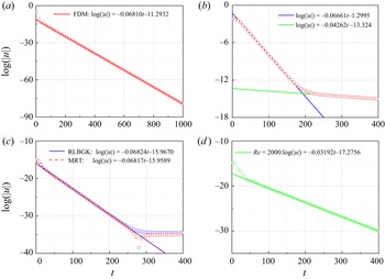
Both the direct numerical simulations (DNSs) and the solver of LNS equations of thermal convection flows are performed using the computational fluid dynamics solver Palabos (version 2.1) (Latt et al. Reference Latt2021). It is well known for its efficient parallelization and second-order accuracy using the MRT model. In the current work, the time step Δt is determined by the Courant–Friedrichs–Lewy condition with the target Courant number being 0.005. The mesoscopic boundary conditions of non-equilibrium extrapolation (Guo et al. Reference Guo, Zheng and Shi2002c; Luo et al. Reference Luo, Wu, Yi and Tan2016) are used for the linearized LBM (LLBM). To evaluate the performance of the LLBM for global stability analysis, in Appendix A we reproduce the results of Pérez et al. (Reference Pérez, Aguilar and Theofilis2017) for the case of 2-D lid-driven flow at Re = 1000. It is seen that non-hydrodynamic mode occurs for lid-driven flow at Re = 1000 due to the defects of mesoscopic boundary conditions. However, for the flow around the criteria Rec or Rac, considered in this work, non-hydrodynamic mode does not occur. Detailed results and discussions are presented in Appendix A. The steps of using the LLBM solvers are summarized below.
Step 1: calculate the baseflow/mean flow, using the LBM as the DNS solver. Note that the accuracy of the DNS solver will influence the linear results directly. So, we use the MRT model for all DNSs.
Step 2: calculate the linear results by LLBM solver. Add a hydrodynamic random perturbation as the initial condition, and then evolve it by time. Here we use the MRT model.
3. Results and discussion
3.1. Global linear instability (as a validation step)
In this section, we first present the results of the grid independency test and validation for the current thermal convection DNS solver. For 2-D natural convection, the maximum velocity Umax is computed with parameters Pr = 7 and Ra = 5 × 10⁶. The results of grid independence are shown in table 1. It is found that the relative errors between resolutions of 256 × 256 and 512 × 512 are less than 0.01 %. Therefore, a resolution of 256 × 256 is applied in the following 2-D numerical simulations considering both accuracy and computational efficiency. For different remaining aspect ratios A, the number of grids in the vertical direction remains constant, while the number of grids in the horizontal direction increases with A.
Grid independency test for 2-D natural convection for Pr = 7 and Ra = 5 × 10⁶.

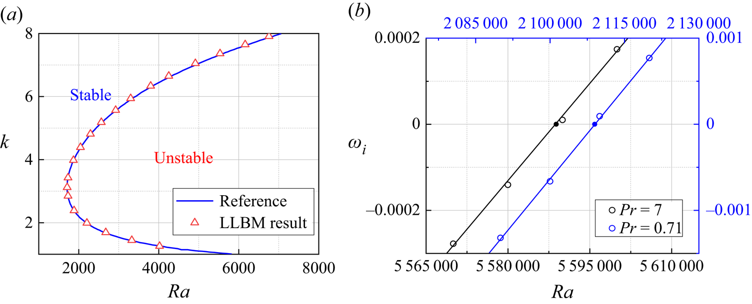
As the first step of validation, we verify the linear instability of the classic RBC (Bergé & Dubois Reference Bergé and Dubois1984) under the global frame. Under the condition of a steady flow field u = 0 (i.e. no fluid motion), the nonlinear equations (2.3) obtain a steady hydrostatic solution by directly solving ordinary differential equations (2.3b) and (2.3c). The linear solver using the LLBM has been tested against linear stability analysis by Bergé & Dubois (Reference Bergé and Dubois1984) in terms of Rac as shown in figure 1(a). In this example, the linear boundary conditions (2.5a) with the periodic boundary on the lateral walls are applied in the linear solver. The domain range is again set to [0, 2 ${\rm \pi}$/k] in the x direction and [0,1] in the z direction. In detail, pitchfork bifurcation occurs at a critical Rayleigh number of Rac = 1711.2 with a critical wavenumber of kc = 3.12. The difference is 0.20 % compared with the reference value of 1707.8.
(a) Neutral stability curve of RBC compared with that of Bergé & Dubois (Reference Bergé and Dubois1984). (b) The critical value of the natural convection: Pr = 7 at Rac = 5 588 857; Pr = 0.71 at Rac = 2 109 003.

Next, the accuracy of simulating the dynamics in the nonlinear equations (2.3) is tested by numerically evolving them to calculate the linear criteria. Both the SRT model and MRT model are used, and table 2 summarizes the results of the DNS. Then, we seek the image part of the eigenvalue and the shape of the eigenfunction of the most dangerous mode. First, the linear stability criteria Rac under two different Prandtl numbers Pr = 0.71 and Pr = 7 are calculated by the LLBM solver, and the image part of the eigenvalue is shown in figure 1(b). By applying the standard linear least squares method, the critical Rayleigh numbers are found to be approximately Rac = 2 109 003 and Rac = 5 588 857 for Pr = 0.71 and Pr = 7, respectively. The former value is very close to the result obtained from the nonlinear equations, as well as to the linear critical value predicted by Xin & Quéré (Reference Xin and Quéré2001) using the spectral method with an error less than 0.01 %. Our method gives a larger difference of 0.5 % for Pr = 7 because of the limitations of the LBM for higher parameter flow. Pérez et al. (Reference Pérez, Aguilar and Theofilis2017) have proven through lid-driven flows that the MRT model shows higher accuracy in DNS and the calculation of LNS equations than the SRT model. Our results show that the same conclusion is reached for thermal convection. Hereafter, all calculations in this study are performed with the MRT model. The eigenfunctions of temperature are presented in figure 5.
Comparison of critical Rayleigh number Rac for Pr = 0.71 and Pr = 7.0. The results of DNS by SRT and MRT models and linear instability analysis by LLBM are compared with those of Xin & Quéré (Reference Xin and Quéré2001).

3.2. Asymptotic energy analysis of RBC in a 2-D rectangular cavity
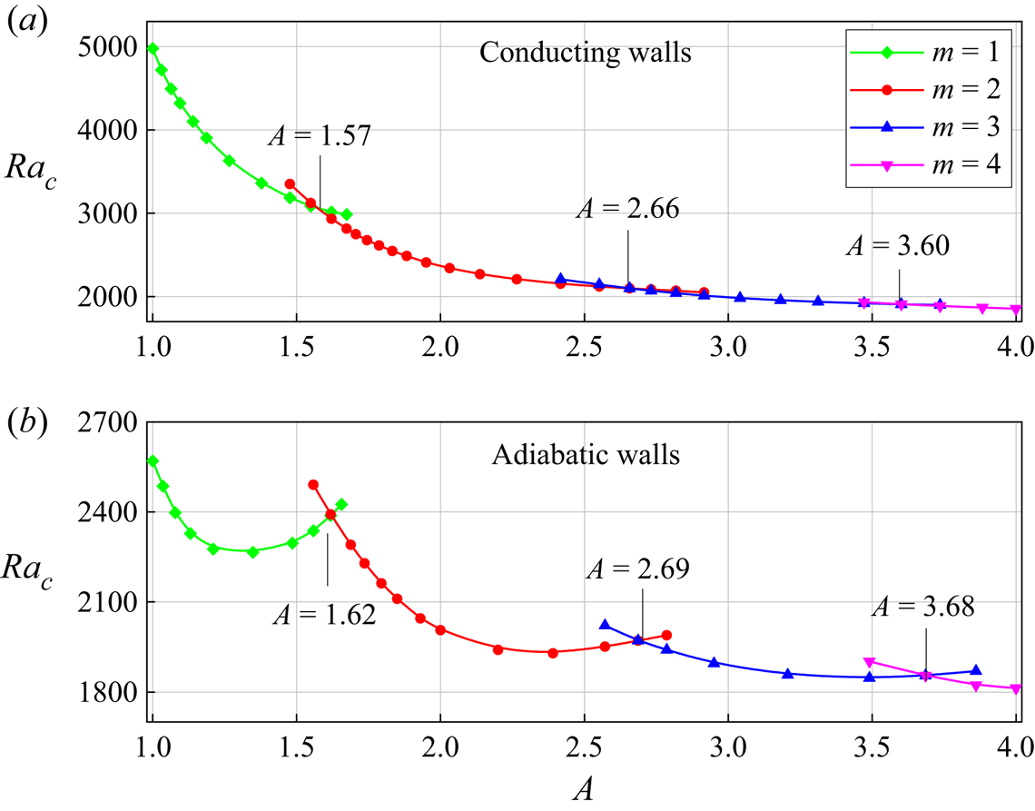
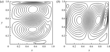
In this section, we investigate the influence of vertical boundaries and aspect ratio on the onset of RBC in a closed 2-D box. Both conducting and adiabatic vertical sidewalls are considered. In order to better understand the bifurcation behaviour of RBC when varying the aspect ratio and the boundary types, it is worthwhile to have a look the mode behaviour that corresponds to linear stability analysis. Figure 2 shows the linear stability threshold Rac as a function of A for both conducting and adiabatic vertical walls. The number m on every branch corresponds to the number of convection cells that appear at the instability threshold. The eigenfunction provides the pattern of the flow for which (locally near this bifurcation point) the motionless solution will be unstable, as shown in figure 3. In addition, there are certain values of A where linear theory is ambiguous in predicting the fastest growing pattern. Figure 2 shows the values of these aspect ratios, so-called double points (Dijkstra Reference Dijkstra1992), in which two patterns become unstable at the same value of Ra. For conducting walls, the 1-cell and 2-cell patterns become simultaneously unstable at A = 1.57; for the 2-cell and 3-cell patterns, this occurs at A = 2.66; for the 3-cell and 4-cell patterns, this occurs at A = 3.60. For adiabatic walls, these double points occur at A = 1.62, A = 2.69 and A = 3.68, respectively.
Linear stability criterion Rac versus A for Pr = 0.71 with (a) conducting and (b) adiabatic vertical sidewalls. The numbers m on every branch are the number of convective cells of the eigenfunction.

The patterns of the most unstable mode for (a) adiabatic walls at Ra = 2250, Pr = 0.71 with A = 1.2 and (b–d) conducting walls at Ra = 4000, Pr = 0.71 with A = 1.2, 1.4, 1.6.

It is obvious that double points for conducting walls are smaller than those for the adiabatic walls case. A comparison of the patterns for the adiabatic boundary and conducting boundary at the same A = 1.20 is shown in figures 3(a) and 3(b), which indicates that there are larger corner eddies for the conducting case. A detailed bifurcation analysis of the influence of A can be explained from the pattern for conducting walls shown in figure 3. There are four small corner eddies, and the eddies grow with increasing A, as shown in figure 3(b–d). When A is beyond the double point (A = 1.57), two eddies at the same sidewall merge, and a sandwich structure (Metzener Reference Metzener1986) appears. This symmetric structure is unstable, and it will be broken by a small-amplitude disturbance, and then flow transition to a structure of two cells. This process arises corresponding to a larger double point (A = 1.62) in the case of an adiabatic boundary.
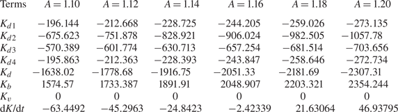
Moreover, solution branches (m = 1, 2, 3, 4) have different monotonicity for these two boundaries at the range of A∈[1, 4], i.e. Rac decreases monotonically with an increase of A for conducting walls, while Rac is non-monotonic in the case of adiabatic walls. Luijkx & Platten (Reference Luijkx and Platten1981), Metzener (Reference Metzener1986) and Gelfgat (Reference Gelfgat1999) also found this phenomenon in a 2-D rectangular box numerically. Physically, Davis (Reference Davis1967) explained the monotonic/non-monotonic nature by associating the energy transfer between the bottom and the top plates with the feature of the convective cell, which lacks quantitative analysis. Therefore, we try to further explain this phenomenon by combining the asymptotic energy analysis, as is widely used in thermal convection (Wanschura, Kuhlmann & Rath Reference Wanschura, Kuhlmann and Rath1996; Wang et al. Reference Wang, Ma, Chen and Sun2012). To obtain the asymptotic energy budget, we choose the most unstable mode as the initial condition and keep the perturbation kinetic energy density equal to 100. After time evolution for 200 non-dimensional time units, the quantitative results are listed in tables 3 and 4, with the notation Kd = Kd 1 + Kd 2 + Kd 3 + Kd 4 and, likewise, Kv = Kv 1 + Kv 2 + Kv 3 + Kv 4. Immediately, one can make several direct observations. First, the only term that can lead to growth in the hydrodynamic perturbation energy density K is linked to the energy transfer from the thermal field, Kb. Second, since the RBC is hydrostatic, there is no production from the baseflow, Kv = 0. Viscous dissipation Kd is always negative for the hydrodynamics to suppress the destabilizing effect of Kb. For the case of conducting walls at Pr = 0.71 and Ra = 4000, we first select the solution branch m = 1 and find Kd 1, Kd 2, Kd 3, Kd 4 and Kb all increase monotonically in magnitude with A from 1.1 to 1.2 as shown in table 3. Under their combined action, dK/dt increases monotonically and beyond 0 (a symbol of pitchfork bifurcation) when A > 1.16. The same phenomenon occurs for any case near Rac at a particular m, which is the reason why the neutral curve is monotonic at A∈[1, 4].
Energy budget for modal instability of RBC for different values of A with conducting walls. The parameters are Pr = 0.71, Ra = 4000.

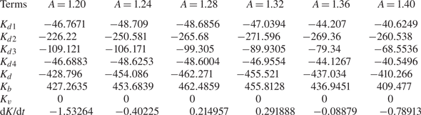
Energy budget for modal instability of RBC for different values of A with adiabatic walls. The parameters are Pr = 0.71, Ra = 2250.

Chandrasekhar (Reference Chandrasekhar1981) indicated the inherent non-monotonic nature of neutral curve branches for RBC with periodic boundary (figure 1a) by a derivation of the analytical expression of different stability curve branches. For the case of adiabatic sidewalls, this non-monotonic characteristic is also apparent. Here, we fix the parameters Pr = 0.71 and Ra = 2250, and change A from 1.2 to 1.4. Due to the reverse mechanism of Kd and Kb, it is reasonable to only care about the change in Kd along A. The most efficient mechanism seems to be related to the terms Kd 2 and Kd 3, which take 78 % of Kd shown in table 4. Kd 2 is the leading stabilizing term, Kd 3 is the second stabilizing term and the effects of Kd 1 and Kd 4 are weaker than those of the previous two. We neglect the effects of Kd 1 and Kd 4 because both of these terms take a percentage of near 11 % of Kd and are slightly independent of A.
When A = 1.20, the magnitude of Kd 3 is almost half that of Kd 2, and the stabilizing is due to the combination of these two terms. However, the effect of stabilizing decreases rapidly and monotonically for Kd 3 from −109.121 at A = 1.20 to −68.554 at A = 1.40. Although the effect of stabilizing is increasing for Kd 3, the total effect of stabilizing decreases and does not inhibit the destabilizing effect of Kb, which may excite the flow. The flow becomes stable again when A > 1.35, for which Kd 3/Kd 2 take a percentage of less than 30 %, and the flow is mainly controlled by Kd 2. By continuing to increase A, all terms decrease monotonically in magnitude, and dK/dt (<0) also decreases monotonically. Combining these energy analysis results and the feature analysis of convective rolls by Davis (Reference Davis1967), a conclusion can be drawn that both narrow, tall cells and wide, flat cells are more efficient for viscous dissipation. The stability curve has a finite minimum corresponding to moderate-sized cells (A = 1.30) being preferred.
3.3. Properties of the DNS and LNS solutions for 2-D natural convection in a square cavity
The instability mechanisms of fluid with different Prandtl numbers for natural convection in a differentially heated square cavity with conducting horizontal walls are here investigated from Pr = 0.01 to Pr = 10. Horizontal rigid walls are conducting, which have a linear baseflow temperature profile of θ(x,0) = θ(x,1) = 1 − x. Two kinds of initial conditions are typically used for the DNS (Gelfgat & Tanasawa Reference Gelfgat and Tanasawa1994):
 \begin{equation}\left. {\begin{array}{*{20}{l@{}}} {\textrm{Zero}\;\textrm{temperature}\;\textrm{field}\;\textrm{(zero}\;\textrm{IC)}:\textrm{ }\theta (x,\textrm{ }z) = 0,}\\ {\textrm{Analytical}\;\textrm{temperature}\;\textrm{field}\;\textrm{(non - zero}\;\textrm{IC)}:\textrm{ }\theta (x,\textrm{ }z) = 1 - x.} \end{array}} \right\}\end{equation}
Before discussing the calculation results, the symmetry of the DNS and LNS solutions are first shown. Due to the symmetry of the boundary condition, the 2-D baseflow admits the anti-symmetry property  $\varPhi$b(x, z, t) = −
 $\varPhi$b(W − x, H − z, t) with
 $\varPhi$ = [u, v, θ − θref]. Solutions φ = [u, v, θ] of the LNS equations admit the following two types of symmetry with respect to (x = W/2, z = H/2):
 \begin{equation}\left. {\begin{array}{*{20}{l@{}}} {\textrm{Symmetry}\;\textrm{(S - mode): }\varphi (x,z,t) = \varphi (W - x,H - z,t),}\\ {\textrm{Anti - symmetry}\;(\textrm{A - mode})\textrm{: }\varphi (x,z,t) ={-} \varphi (W - x,H - z,t).} \end{array}} \right\}\end{equation}
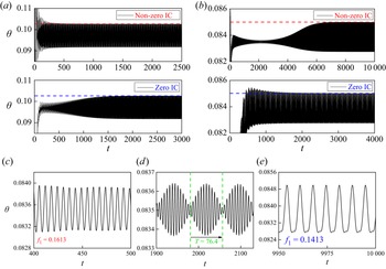
These symmetries can be broken through bifurcations. Here temperature θ is plotted over time at a location on the top right side of the conducting wall (0.9, 0.9). Both the zero IC and non-zero IC converge to the same mean amplitude and high oscillation frequency, but for the length of time simulated, differences persist in Pr = 0.71 and Pr = 7, and a comparison of these solutions can be seen in figures 4(a) and 4(b). For Pr = 7 and Ra = 5.69 × 10⁶ with a non-zero IC, it is clear that in the developing flow there are two frequencies of oscillation present: a high-frequency mode with f 1 = 0.1613 and a low-frequency mode with f 1 = 0.1413. The relative strength of the two modes varies over t = 0–7000. The energy in the high-frequency mode increases over t = 0–3000 and then decreases over t = 3000–7000. From t = 7000, the high-frequency mode is largely dissipated and the mean flow asymptotically approaches a final solution, as illustrated in figure 4(e). Gelfgat & Tanasawa (Reference Gelfgat and Tanasawa1994) first studied this problem using the non-zero IC; however, they obtained an incorrect result for the critical frequency with a higher frequency fc = 0.1614. It may be that the convergence condition is so large that the convergence occurs at the multimodel oscillation step shown in figure 4(d). The low-frequency mode was excited directly by the zero IC, so a rather short simulation time was needed, only less than 2000, compared with the non-zero IC with a time of more than 7000.
Time-evolution series for two Prandtl numbers: (a) Pr = 0.71 with Ra = 2.14 × 10⁶ and (b) Pr = 7 with Ra = 5.69 × 10⁶. The enlarged plots of (b) with non-zero IC illustrate (c) the initial developing flow, (d) the multimodel oscillation in the initial development flow and (e) the dominant mode of oscillation at full development.

Note that with non-zero IC, the flow reaches the saturated oscillation state at less than t = 1000, while the zero IC needs an integral over 2000 non-dimensional time at Pr = 0.71 and Ra = 2.14 × 10⁶, as shown in figure 4(a). Hydrodynamic behaviour is opposite for the case of Pr = 7. It has been proven that the nonlinear saturated perturbation has the same symmetry as the leading eigenmode and a similar structure around the critical value, i.e. comparing the DNS result of Henkes & Quere (Reference Henkes and Quere1996) and the LNS result of Xin & Quéré (Reference Xin and Quéré2001). Comparing the zero IC and the non-zero IC, the symmetric non-zero IC contributes to more energy on exciting the S-mode than the zero IC, i.e. if the leading mode of the convection is S-mode, flow will reach the saturated oscillation state faster using the non-zero IC. Therefore, determining the symmetry of the most unstable mode for natural convection with different Prandtl numbers has economic value for numerical simulation.
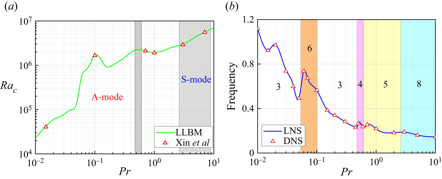
Therefore, abundant simulations are performed to determine the symmetry of the leading mode under different Prandtl numbers. Figure 5 shows the relationship between the linear critical Rayleigh number Rac and critical frequency fc for different Pr values from 0.01 to 10. The critical Rayleigh number increases monotonically with the Prandtl number except in the range 0.1 to 1. The shaded zones in figure 5(a) indicate that the most unstable mode is symmetric which takes place in two intervals, Pr = [0.47, 0.61] and Pr = [2.6, 8.8], and the other Prandtl number cases exhibit anti-symmetry. The unstable spatial mode structure of the eigenfunction  $\hat{\theta }$ (perturbed temperature) is presented in figure 6 for three selected values Pr = 0.3, 0.71 and 7.0. The time-averaged temperature and flow fields (mean flow) are taken to be the baseflow. The usual typical flow features, i.e. thin vertical boundary layers as well as stratified core regions, are evident for the mean flow, which admits the anti-symmetry property. An animation of the perturbation temperature reveals that the perturbation was travelling in a clockwise direction through the horizontal and vertical boundary layers. The oscillatory behaviour is present along the partition wall with perturbations being amplified on both sides of the wall in the direction of flow. The perturbations are advected from the vertical walls onto the horizonal intrusions, where there is strong dissipation and the magnitude of the perturbations is rapidly reduced.
(a) The linear critical Rayleigh number Rac with Prandtl number Pr compared with the result of Xin & Quéré (Reference Xin and Quéré2001). The shaded zones represent the symmetry leading mode (S-mode), which are Pr = [0.47,0.61] and Pr = [2.6,8.8], and the other zone represents the anti-symmetry leading mode (A-mode). (b) The critical frequency f represented by the DNS result and linear stability analysis. The numbers (i.e. 3, 4, 5, 6 and 8) represent the number of wave structures.

The spatial distribution of the mean flow and corresponding most unstable mode at (a,d) Ra = 1.54 × 10⁶ and Pr = 0.3; (b,e) Ra = 2.108 × 10⁶ and Pr = 0.71; and (c,f) Ra = 5.573 × 10⁶ and Pr = 7.

Figure 5(b) shows that the first 2-D instability is due to a supercritical Hopf bifurcation (branching from a steady solution to a periodic unsteady solution, ωi = 0, ωr ≠ 0). The general trend of fc with the Prandtl number is opposite to that of Rac, which decreases from 1.1 at Pr = 0.01 to 0.2 at Pr = 10. The nonlinear oscillatory critical frequencies calculated by DNS are same as the linear results. If the combination of a positive and a negative temperature patch in a clockwise direction is defined as one structure, the most unstable modes consist of at least three structures. Gill (Reference Gill1966) suggested that the boundary layer thickness scale is equal to HRa −1/4, the boundary layers are thinner and the wave structures are smaller in the boundary layers. For low Prandtl numbers (Pr < 0.1), the ratio of the thermal diffusion rate to the momentum diffusion rate is beyond 10. There are thicker thermal boundary layers and only three wave structures for Pr < 0.054. Three pairs of wave structures are compressed and broken to six smaller structures, and the broken structures will be saturated corresponding to a higher critical Rayleigh number. When 0.11 < Pr < 0.54, the system reverts to three pairs of wave structures, i.e. Pr = 0.3 and Ra = 1.54 × 10⁶ as shown in figure 6(d). The anti-symmetry leading mode is replaced by a symmetry mode with four wave structures in the range from 0.45 to 0.6, and that also occurs at Pr = 2.6, where the anti-symmetry mode changes to the symmetry mode, i.e. Pr = 7 and Ra = 5.573 × 10⁶ as shown in figure 6(f). There are more wave structures (eight travelling waves) observed along the cavity boundary layer. However, the wave structures are less regular than those at Pr = 0.71 and Ra = 2.108 × 10⁶, as shown in figure 6(e), and very small structures are obtained along horizontal walls.
The EVP is also investigated by monitoring the time trace of perturbation quantities  $\theta ^{\prime}$ and
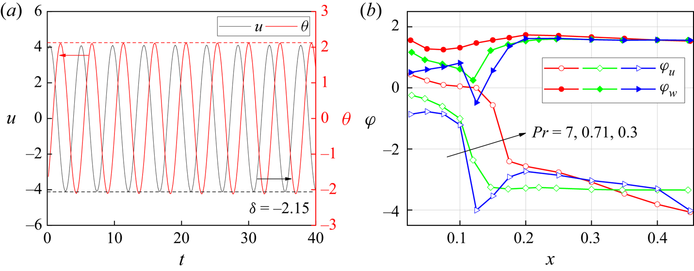
 $u^{\prime}$ along the normal direction of the vertical boundary from (0, 0.5) to (0.5, 0.5). The time trace in figure 7(a) shows that the temperature perturbation
 $\theta ^{\prime}$ lags the velocity perturbation
 $u^{\prime}$ by a constant phase difference δ = 2.15 at Ra = 2.108 × 10⁶ and Pr = 0.71 and x = 0.11. In addition, velocity and temperature perturbations share the same exponential ascending slope and increase slightly with Ra, such that ωi ,θ = ωi ,u = ωi. There is a different hydrodynamic behaviour in the boundary layers and the core zone, which causes a various lag in these two zones, as shown in figure 7(b). A phase difference δu is defined as
 ${\delta _{\boldsymbol{u}}} = \delta (\theta ^{\prime})-\delta (\boldsymbol{u^{\prime}})$, and perturbation velocity
 $v^{\prime}$ shows a phase lead rather than velocity u reflecting a phase lag. The phase lag δv was also found in the work of Ke et al. (Reference Ke, Williamson, Armfield, Mcbain and Norris2019), who researched the stability of a temporally evolving natural convection boundary layer on an isothermal wall. Along the x direction a phase step occurring at x∈[0.1,0.2] causes a larger lead/lag δu at x > 0.2 (core zone) than x < 0.1 (boundary layers). This phenomenon can be explained by the eigenfunctions in figure 6. There is a positive temperature patch on the vertical boundary and a corresponding negative structure attached to it in the core region. The positive patch is thinner for larger Prandtl numbers and the phase step will occur in the order of Pr = 0.3, Pr = 0.71 and Pr = 7.
(a) The development of the perturbation quantities θ and w at x = 0.11. (b) The phase differences δ between u and θ at Ra = 5.573 × 10⁶ with Pr = 7, Ra = 2.108 × 10⁶ with Pr = 0.71 and Ra=1.54 × 10⁶ with Pr = 0.3 are plotted against the horizontal location at the vertical location, y = 0.5.

3.4. Energy analysis for 2-D natural convection
Because natural convection consists of different high-Rayleigh-number structures, several more-or-less fundamental physical instability mechanisms are possible. The most unstable one (with the lowest critical Rayleigh number, Rac) depends on the type of boundary conditions on the horizontal walls. For the conducting case, the first instability is related to Rayleigh–Bénard instability (Henkes & Hoogendoorn Reference Henkes and Hoogendoorn1990) because the temperature at horizontal walls introduces a local region with unstable stratification. Instability mechanisms and the local region instability for different Prandtl-number flows are studied by asymptotic energy analysis in this section.
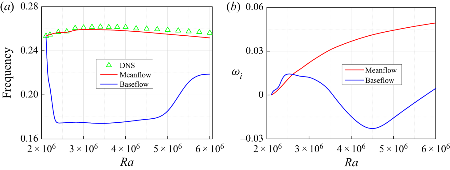
These time-averaged fields are obtained in the usual manner by computing an arithmetic mean of the instantaneous fields over 100 oscillation periods. The prediction of the weakly nonlinear hydrodynamics through global linear analysis is presented in figure 8. In the case of wake flows, Hammond & Redekoop (Reference Hammond and Redekoop1997) and Pier (Reference Pier2002) have noted that a linear criterion applied to the mean flow, and not to the baseflow, yields particularly good results for the prediction of the frequency of the unsteadiness. Barkley (Reference Barkley2006) and Sipp & Lebedev (Reference Sipp and Lebedev2007) confirmed this result using a global linear analysis, and showed in addition that the mean flow was marginally stable. We draw the same conclusion for the natural convection, as shown in figure 8. Figures 8(a) and 8(b) respectively represent the pulsation and amplification rate of the eigenmode as a function of Rayleigh number at Pr = 0.71. We also sketch the DNS pulsation as a comparison in figure 8(a). It appears clearly that the mean-flow calculations yield the true nonlinear frequency and amplification rate (no DNS result given because of measurement difficulties) at the weakly nonlinear range [Rac, 2Rac]. However, the baseflow predicts rather incorrect results. Therefore, in this work, we use the mean flow for linear stability calculations when Ra is slightly above the critical conditions and only use the baseflow for steady flow cases, which provides a better guarantee of the validity of stability analysis in all cases.
(a) Comparison of the critical frequency (eigenvalues) of the LNS result and the critical oscillatory frequency of the DNS result. The red line represents taking the mean flow as the baseflow and the blue line is unstable instantaneous baseflow. (b) The results of increasing rate ωi over Ra at Pr = 0.71 and Ra∈[2 × 10⁶, 6 × 10⁶].

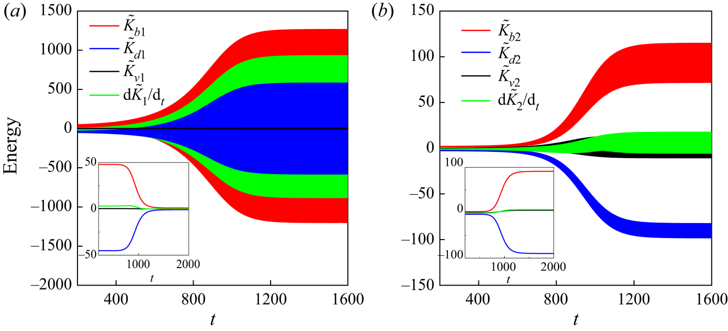
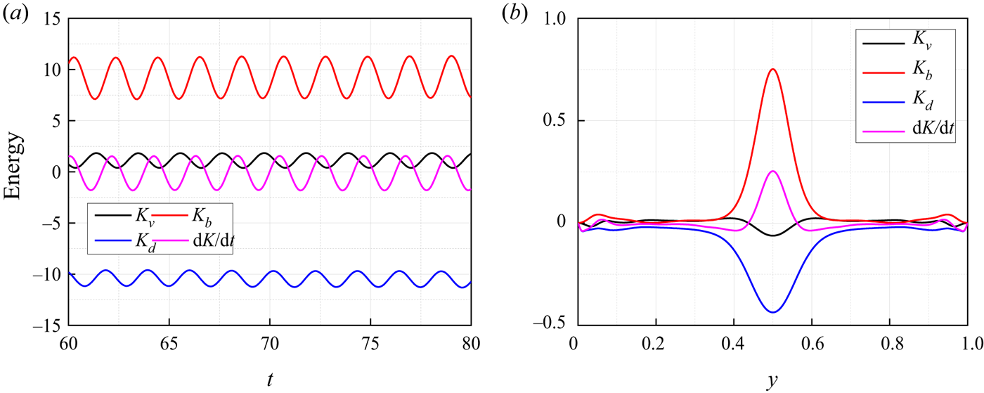
The nonlinear turbulent energy increase is checked to monitor different terms for (2.26) from the onset of unstable  $(\textrm{d}\tilde{K}/\textrm{d}t > 0)$ to saturated oscillatory
 $(\textrm{d}\tilde{K}/\textrm{d}t = 0)$ behaviour. The mean field at Ra = 2.2 × 10⁶ is used as the initial condition. Before reaching the saturated oscillatory state, the perturbation first goes through linear energy growth and then nonlinear rise. Figure 9 shows the time evolution of the nonlinear turbulent energy for the first- and second-order terms. The higher third-order term N 3 is negligible, which takes place at a magnitude less than 0.01 compared with the former two terms. First-order perturbation energy terms
 ${\tilde{K}_{b1}}$,
 ${\tilde{K}_{d1}}$ and
 ${\tilde{K}_{v1}}$ are calculated over time, and the inset in figure 9(a) gives the mean magnitude of these terms. Although there is a large amplitude for these terms, the mean influence retains a small magnitude, i.e. the maximum amplitude of
 ${\tilde{K}_{b1}}$ is 1240 with a mean value of 4.9 at t = 1500. Figure 9(b) shows the development of the second-order perturbation energy terms
 ${\tilde{K}_{b\textrm{2}}}$,
 ${\tilde{K}_{d\textrm{2}}}$ and
 ${\tilde{K}_{v\textrm{2}}}$, and the nonlinear rise occurs when t > 700. The result shows that the initial phase of unsteadiness is mainly controlled by the first-order term
 $\textrm{d}\tilde{K}/\textrm{d}T > \textrm{1}0$ for t < 700. After that, second-order terms replace the dominant position until the oscillation is saturated. Terms
 ${\tilde{K}_{b1}}$ and
 ${\tilde{K}_{b\textrm{2}}}$ are the leading unstable terms, which indicates occurrence of instability with a buoyancy mechanism.
The time evolution of the nonlinear energy analysis at Pr = 0.71 and Ra = 2.2 × 10⁶. (a) First-order terms and (b) second-order terms.

Asymptotic energy analysis dictates the growth rate of the most unstable mode. We seek to connect the asymptotic energy analysis to the nonlinear turbulent energy at Ra = 2.2 × 10⁶ and Pr = 0.71. Contributions to the local growth rate of the asymptotic kinetic energy are achieved through mechanisms of various budget terms from (2.30). Asymptotic energy and the second-order turbulent energy terms are also exemplified in the first and third rows of figure 10. The positive value denotes the amplification of the perturbation from the respective terms, i.e. the flow is destabilizing, while the negative value corresponds to stabilizing. Figure 10(a 2–c 2) gives the spatial distribution of the total energy terms  $\textrm{d}\tilde{K}/\textrm{d}t$,
 ${\tilde{K}_b}$ and
 ${\tilde{K}_v}$. Although the distribution of the total turbulent energy terms differs from that of the asymptotic energy budget terms to some extent, the total effect of destabilizing due to first-order terms
 $\textrm{d}{\tilde{K}_\textrm{1}}/\textrm{d}t$ is small enough compared with the second-order terms
 $\textrm{d}{\tilde{K}_\textrm{2}}/\textrm{d}t$ when t > 700. In this work, we are solely concerned with the saturated oscillation behaviour of perturbation and can ignore the effect of first-order terms. The distribution of second-order turbulent energy is almost the same as that of asymptotic energy. Therefore, we can use asymptotic energy analysis to predict the local region instability with oscillatory flow.
Contributions to the local growth rate of the perturbed kinetic energy through mechanisms of various budget terms at Ra = 2.2 × 10⁶, Pr = 0.71 (red, destabilizing; blue, stabilizing). Asymptotic energy analysis with (a1) dK/dt; (b1) Kb; (c1) Kv. Turbulent energy analysis of the total contributions of the perturbed kinetics with (a2)  $\textrm{d}\tilde{K}/\textrm{d}t$; (b2)
 ${\tilde{K}_b}$; (c2)
 ${\tilde{K}_v}$. Second-order term with (a3)
 $\textrm{d}{\tilde{K}_\textrm{2}}/\textrm{d}t$; (b3)
 ${\tilde{K}_{b\textrm{2}}}$; (c3)
 ${\tilde{K}_{v\textrm{2}}}$.

Figure 10(a 1) shows the stabilizing and destabilizing regions at Ra = 2.2 × 10⁶ and Pr = 0.71, which can be divided into the core zone and boundary layers. The magnitude of dK/dt in the core zone is always negative, so this region is stabilizing. For boundary layers, a larger magnitude of dK/dt is observed in vertical boundary layers compared with horizontal layers. Then, the transition may be due to the perturbation being excited at vertical boundary layers. Fluid viscosity apparently stabilizes the flow, and is most effective around the corner in vertical walls (Kd not given here). Terms Kv and Kb play a role in destabilizing, as shown in figure 11(c). The destabilizing effect of Kv is weaker compared with the buoyancy term Kb, but it is effective in a narrower area in vertical boundary layers, as shown in figures 10(b 1) and 10(c 1). Both of these terms affect the perturbed flow in a more complex manner: they may stabilize and destabilize the flow in different regions. First, at the lower left (top right) corner of the cavity, the flow is primarily stabilized by the inertial term but destabilized by the buoyancy term. Then, at the top left (lower right) corner of the cavity, both the inertial term Kv and buoyancy term Kb contribute to the steady flow transition to oscillation. Flows at the middle section of the vertical boundary layers are generally stabilized by all three terms.
(a,b) Contributions to the local growth rate dK/dt of the asymptotic perturbed kinetic energy through mechanisms of various budget terms with Pr: (c) at Ra = 2.108 × 10⁶ and Pr = 0.71; (d,e) at Ra = 5.573 × 10⁶ and Pr = 7.

The role of energy budget terms (stabilizing or destabilizing) and their magnitudes are dependent on Prandtl numbers. Although the effect of Pr is only reflected by the temperature term, it will change the mean-flow field and consequently all budget terms in an indirect way, as comparably analysed and quantitatively presented in figure 11. Then, perturbation is neutral at the critical stable state and the asymptotic kinetic energy balance is
 \begin{equation}0 = {K_v} + {K_b} + {K_d}.\end{equation}
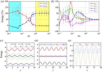
We study the effect of the destabilizing terms Kv and Kb for different Prandtl-numbers flows, as shown in figure 11(a). Asymptotic energy is normalized by Kd, and we obtain  ${K_b}/{K_d} ={-} {K_v}/{K_d}$. For Pr < 0.08 (thermal diffusion rate is faster than the momentum), Kv is the only destabilizing term, and thermal diffusion probably has the same scale and function as the viscous dissipation. On increasing the Prandtl number to Pr < 0.44, Kv is the dominantly destabilizing term. And it combines with the destabilizing buoyancy term Kb, both of these terms adding to the transition. Instability due to the buoyancy effect begins to replace the inertial mechanisms and becomes the first important destabilizing factor when Pr > 0.44. The term Kv stabilizes the flow when Pr > 1, and the ratio Kv/Kb remains stable around a constant value. For RBC, Touihri, Ben Hadid & Henry (Reference Touihri, Ben Hadid and Henry1999), Gelfgat, Bar-Yoseph & Solan (Reference Gelfgat, Bar-Yoseph and Solan2000) and Ma, Henry & Ben Hadid (Reference Ma, Henry and Ben Hadid2005) showed that the flow becomes oscillatorily unstable due to inertial mechanisms for low-Prandtl-number fluids (Pr = 0.02), and it is due to thermal mechanisms for high-Prandtl-number fluids (Pr = 1). These conclusions are consistent with the case of natural convection here. Therefore, the instability mechanisms may be an inherent property for different Prandtl-number fluids and the value of Kv/Kb will be slightly affected by the baseflow, i.e. only a small difference of it in 2-D natural convection and 3-D natural convection for Pr = 0.71, as shown in figures 11(a) and 16(a).
The positive or negative value and magnitude of Kv depend on the baseflow and have no regularity with Pr, as shown in figure 11(b). In general, Kv 2 is the leading destabilizing term and Kv 3 is the second destabilizing term for Pr < 0.1. However, Kv 3 becomes the dominant destabilizing term and Kv 4 stabilizes the flow for Pr > 0.1. In detail, we quantitatively illustrate Kv for two different Prandtl-number cases, i.e. Pr = 0.71 and 7. Figure 11(c) shows that Kv 3 is the first destabilizing term, Kv 1 is the second destabilizing term and Kv 2 becomes slightly stabilizing and the effect (magnitude) is weaker than the previous two; Kv 4 is always the most dominantly stabilizing term for these two Prandtl-number cases at Ra = 2.108 × 10⁶ and Pr = 0.71. Figure 11(e) shows the corresponding kinetic energy fluctuation analysis at Ra = 5.573 × 10⁶ and Pr = 7. Term Kv 3 is still the leading destabilizing term and Kv 1 follows. Kv 2 has a minimal destabilizing effect compared with Kv 3 and Kv 1.
3.5. Three-dimensional natural convection
3.5.1. Subcritical bifurcation for low-Prandtl-number natural convection
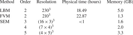
The 3-D physical model is built by adding another two conducting rigid walls at y = 0 and A. Before presenting the 3-D results, it is worth comparing the performance of our LBM solver with that of other mainstream computational fluid dynamics solvers. The same calculation environment is kept, i.e. Courant number of 0.005 and parallel with 8 CPU cores. A relative error of 0.1 % of the vorticity at the centre of the cavity (0.5, 0.5, 0.5) is selected as the grid independence criterion at Ra = 1 × 10⁵ and Pr = 0.71. Then, we calculate the minimum resolutions used for three solvers, i.e. Palabos, OpenFOAM (version 9.0) (Jasak, Jemcov & Tukovic Reference Jasak, Jemcov and Tukovic2007) based on the FVM and Nek5000 (version 19.0) (Fischer, Kerkemeier & Peplinski Reference Fischer, Kerkemeier and Peplinski2008) based on the SEM. Theoretically, both LBM and FVM have the same second-order accuracy. While for SEM, we select the third-, fourth- and fifth-order accuracy, as second order cannot be implemented in Nek5000 (divergency when the number of elements is greater than 18 in one direction). The resolution of the SEM is equal to  ${({R_1} \times {R_2})^3}$, where R 1 is the number of elements in one direction and R 2 is the number of grids in an element. For example, we select a grid resolution of (4 × 5)3 for the fifth-order case, because Error = 0.018 % at (4 × 5)3 but Error = 0.38 % at (3 × 5)3. Minimum resolutions for these three methods are shown in the third column of table 5. After that, we quote the physical time and memory required for the final steady solution to be obtained.
Comparison of Palabos solver, Nek5000 solver and OpenFOAM solver for 3-D natural convection in cubic cavity with Courant number of 0.005 at Pr = 0.71 and Ra = 1 × 10⁵.

As for the simulation condition adopted in this work, the LBM is comparable with the FVM, which involves the same magnitude of physical time. However, neither LBM nor FVM can compare with the SEM in computing speed. The SEM can achieve the same Error with rather few resolutions, and the physical time needed is less than one hour for all third-, fourth- and fifth-order schemes. The advantage of our LBM/LLBM can reflect on flow with complex boundary, i.e. concentric and eccentric annuli (Luo et al. Reference Luo, Yi, Tan and Wu2017) and porous media (Zhao et al. Reference Zhao, Dai, Tang, Qu and Li2010; Jiang, Xu & Zhou Reference Jiang, Xu and Zhou2021), which has potential for further development in practical engineering application.
The abovementioned computational studies are restricted to 2-D instabilities. The instability of 3-D natural convection for a low Prandtl number (Pr < 0.1) is studied in this section. Xin & Quéré (Reference Xin and Quéré2001) first gave the neutral instability curve for 3-D natural convection with periodic boundaries in the y direction at Pr = 0.015, which showed a critical Rayleigh number Rac = 7950 with critical wavenumber kc = 8.15. We extend his work and study the instability in a 3-D closed cavity. A zero IC was selected, and the mean Nusselt Nu at the plane x = 0, 1 was calculated when increasing the Rayleigh number. Figure 12 plots the evolution of Nu versus Rayleigh number Ra, which shows that the stable one-cell flow bifurcates to the stable two-cell flow when Ra > 8059. Two-cell flow transitions to an oscillatory state at Rac 2 = 17 350. Once the two-cell convection is reached, decreasing the value of Ra below Rac 1 (the instability threshold) does not result in the suppression of transition until a small-amplitude criterion Raf = 3768. Therefore, a hysteresis loop associated with these two values of the stability parameter Ra results, which is also a feature of subcritical bifurcation.
Subcritical bifurcation of 3-D natural convection represented by the Nusselt number Nu at A = 1 and Pr = 0.015. Upward-pointing triangles show the continuous increase in Ra, while the downward-pointing triangles present the case of continuous decrease. The blue line represents the one-roll solution, and the red line is the two-roll solution. The dashed line shows the mean Nusselt number of the oscillatory state. Three instability criteria are numerically predicted: Rac 1 = 8059, Rac 2 = 17 350 and Raf = 3768.

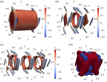
Figures 13(a) and 13(b) show the Q-criterion isosurfaces Q = 0.001 and Q = 0.003 coloured by the y component of the vorticity ranging from −0.2 to 0.2 at the same Rayleigh number Ra = 8000, respectively. The one-cell structure breaks to the two-cell structure with respect to the midplane y = 0.5. Linear instability analysis shows that the first instability criterion (Rac 1) is a type of Hopf bifurcation with a critical frequency fc = 0.24. The linear 3-D equations, together with the boundary conditions specified in (2.5), admit A-mode or S-mode plane symmetry with respect to y = 0.5. The perturbation temperature of the leading mode is given in figure 13(d). Compared with the modal analysis of the RBC in § 3.2, 3-D eggy vortices around the y = 0 and 1 planes also arise with an increase of A and the first instability is related to that. Subcritical bifurcation is also found for the other Prandtl-number case, i.e. Pr = 0.05, Ra = 50 000 and A = 2. Figure 13(c) gives the Q-criterion isosurface Q = 0.05 and coloured by the y component of the vorticity ranging from −0.6 to 0.6.
The Q-criterion isosurfaces (a) Q = 0.001 and (b) Q = 0.003 coloured by the y component of the vorticity ranging from −0.2 to 0.2 for the same parameters: A = 1, Pr = 0.015 and Ra = 8000. (c) The Q-criterion isosurface Q = 0.05 coloured by the y component of the vorticity ranging from −0.6 to 0.6 with A = 2, Pr = 0.05 and Ra = 50 000. (d) The isosurfaces θ = 1, −1 of the first unstable mode corresponding to the baseflow of (a).

3.5.2. Supercritical bifurcation
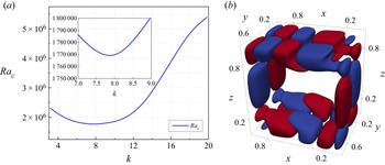
The steady natural convection transitions to periodic oscillation when Ra is beyond the critical value of supercritical bifurcation, i.e. Rac 2 for Pr = 0.015. Here, we research the supercritical bifurcation behaviour for Pr = 0.71 in a cubic cavity (A = 1). There is no reason to assume that 2-D perturbations are less stable than 3-D perturbations, as the existence of a Squire-like principle (Lockett Reference Lockett1969), which holds for forced-convection boundary layers, is unknown for natural convection. Henkes & Quere (Reference Henkes and Quere1996) studied the stability with respect to 2-D and 3-D perturbations of natural convection flow of air in a square enclosure with differentially heated vertical walls and periodic boundary conditions in the lateral direction. They showed that the 2-D modes were more stable than the 3-D ones. The 3-D intrinsic instability effect can be calculated by assuming that the flow is periodic in the y direction under no-slip boundary conditions. In this section, the first purpose is to determine the influence of 3-D waves on the stability of 2-D mean flow. Figure 14(a) shows the neutral instability curve with a wavenumber range from 3 to 20. Instability occurs at critical wavenumber kc = 7.86, corresponding to a critical Rayleigh number  $R{a_c} = 1.77 \times {10^6}$.
(a) The neutral instability curve of 3-D natural convection with periodic boundaries in the y direction for Pr = 0.71. The most unstable wavenumber kc is 7.86 with critical Rayleigh number Rac = 1.77 × 10⁶ and critical frequency fc = 0.263. (b) The distribution of the eigenfunction with perturbation temperature at kc = 7.86.

We calculated and compared eigenpairs in 2-D and 3-D critical modes and found that there was a higher critical frequency fc = 0.263 in the 3-D case compared with fc = 0.254 in the 2-D case. The eigenfunction (temperature) of the 3-D perturbation is shown in figure 14. Based on the distribution of isosurfaces, both cases are characterized by five large structures compared with the 2-D simulation. However, the most important difference is that there is one smaller structure in the vertical boundary layers and at the exiting corners in the 3-D case. According to the snapshot, perturbations in boundary layers were damped before turning the corners and reamplified slightly afterward. The critical wavelength, lc = 2 ${\rm \pi}$/kc, is equal to 0.8 for this case. If there is subcritical bifurcation for this Prandtl number, the length of a convection cell should be slightly larger than lc/2, just like the case in § 3.5.1, i.e. there are four cells and the average diameter is 0.5 for Pr = 0.05, corresponding to a critical wavelength of 0.4. However, even if A = 3, subcritical bifurcation did not occur. We are not sure whether subcritical bifurcation is a property specific for low-Prandtl-number flow.
Therefore, there is only one linear instability criterion Rac = 2.44 × 10⁶ for 3-D natural convection at Pr = 0.71 and A = 1. Under this parameter, an irregular one-roll structure existed based on the temperature and the Q-criterion isosurfaces, as shown in figures 15(a 1) and 15(a 2). The high Q-criterion is mainly distributed at the corner of the boundary layers, but it gathers at the centre of the cavity along the y direction for Pr = 0.015, as shown in figure 13(a). We also focus on the leading mode, and three direction views of the eigenfunction (temperature) are shown in figure 15(b). The S-mode is found not only with respect to the y = 0.5 plane but also in the x–z plane with only four pairs of wave structures. The rigid walls at y = 0 and 1 change the symmetry of the leading mode compared with the 3-D mode with a periodic boundary (A-mode). In addition, the supercritical bifurcation is judged as a type of Hopf bifurcation and the wave structures travel clockwise with a frequency fc = 0.245. The irregular wave structures predict that there is a complex instability mechanism, which is discussed in terms of the energy analysis.
The spatial distribution for the results of DNS, LNS and energy analysis for the same parameters: A = 1, Pr = 0.71 and Ra = 2.44 × 10⁶ (Rac). (a1,a2) The temperature isosurfaces at θ = 0.3 and θ = 0.7 coloured by the velocity magnitude ranging from 0 to 0.4 and the Q-criterion isosurfaces Q = 0.02 coloured by the y component of the vorticity ranging from −0.4 to 0.4, respectively. (a3,c1,c2,c3) Distributions of the energy budgets of dK/dt, Kb, Kv and Kd, respectively. (b1,b2,b3) Three direction views of the isosurfaces at θ = 1 and −1 of the first critical eigenmode.

The time evolutions of the energy budget terms dK/dt, Kb, Kv and Kd are plotted in figure 16(a). The buoyancy term is also the leading destabilizing term, and the value of Kv/Kb is 0.15, which is slightly less than that in the 2-D case. The total perturbed energy budget along the y direction is calculated to study the influence of the sidewalls at y = 0, 1. Figure 16(b) shows that perturbation is excited (dK/dt > 0) around the midplane y = 0.5 from 0.44 to 0.56, where the only destabilizing term is the buoyancy term and both the momentum term and viscosity term stabilize the flow. The spatial distributions of these perturbed energy budgets are shown in figures 15(a 3) and 15(c), which show more fragmented and irregular energy structures compared with the leading mode. They clearly show that the energy distribution gathers in the core region of the cavity around the midplane y = 0.5, especially for Kd.
(a) Energy analysis for Pr = 0.71 with the period boundary and the A = 1 case. (b) Total budget for the kinetic energy along the y direction for Ra = 2.4 × 10⁶ and Pr = 0.71.

4. Conclusions
In this work, we extend a LLBM developed by Pérez et al. (Reference Pérez, Aguilar and Theofilis2017) for global linear stability analysis to thermal convective flow based on the linearization of the local equilibrium PDF. Instead of solving the coupled LNS equation and the energy equation, two different linear lattice Boltzmann equations are formulated. Similar to the time-stepping solvers of the traditional numerical methods to solve the LNS equations, the most unstable mode is extracted. Our LLBM was validated by calculating the linear critical Rayleigh number and the global eigenmodes of 2-D natural convection in a cavity. The results obtained by the MRT model are highly consistent with those obtained by spectral methods, with a difference of less than 1 %.
Asymptotic energy analysis is reasonable to use for researching the instability mechanisms of thermal convection by comparing with nonlinear turbulent energy analysis. It explains the different monotonicity of the neutral instability curve for RBC in a 2-D rectangular cavity. In the case of 2-D natural convection in a square cavity heated from the side, the instability mechanisms for different Prandtl-number fluids are investigated from Pr = 0.01 to Pr = 10. Steady convection transitions to periodic oscillation by Hopf bifurcation due to inertial mechanisms when Pr < 0.44, and buoyancy mechanisms become the leading reason for destabilization for Pr > 0.44. In detail, a low-Prandtl-number fluid (Pr < 0.08) becomes oscillating only due to inertial mechanisms and buoyancy mechanisms stabilize the flow. However, instability mechanisms are reversed for higher Prandtl numbers (Pr > 1). Subcritical bifurcation is found for low Prandtl numbers (Pr < 0.1) with 3-D natural convection, in which one convective cell breaks into two cells in the y direction with a hysteresis loop, and the bifurcation is proven to be a type of Hopf bifurcation. Lastly, the supercritical bifurcation of 3-D natural convection at Pr = 0.71 is also studied. The symmetry of the leading mode is the S-mode with fewer wave structures.
Results in this work prove that the LLBM is a promising tool for global stability analysis owing to its kinetic nature and matrix-free operation. Further works can consider stability analysis using the LLBM for more complex problems by taking the advantage of the LBM in complex geometry and fluids, multifield coupling and multiphase flow.
Acknowledgements
The authors thank colleagues Jing-da Yao and Yu Zhang. All referees are especially acknowledged for their enlightening suggestions that resulted in the improvement of this paper.
Funding
This work is supported by the National Natural Science Foundation of China (grant nos. 51906051 and 52076055) and the Fundamental Research Funds for the Central Universities (grant no. FRFCU5710051020).
Declaration of interests
The authors report no conflict of interest.
Appendix A. Limitations of the LLBM: discussed in terms of 2-D lid-driven flow
For 2-D lid-driven flow at Re = 1000, Pérez et al. (Reference Pérez, Aguilar and Theofilis2017) indicated a spurious numerical mode for long integration time (t larger than 200) by the LLBM with both the SRT model and MRT model. This mode can be judged as a non-hydrodynamic mode through comparing the results calculated by the FDM, i.e. no non-hydrodynamic mode until t = 1000 as shown in figure 17(a). In fact, the collision term is driving the stability and accuracy of LBMs. Then, another high-accuracy numerical model, i.e. the regularized Bhatnagar–Gross–Krook (RLBGK) collision model (Latt & Chopard Reference Latt and Chopard2006), is used to eliminate this non-hydrodynamic mode. The evolution of the RLBGK model for flow motion reads
 \begin{equation}{f_\alpha }(\boldsymbol{x} + {\boldsymbol{e}_\alpha }\varDelta t,t + \varDelta t) = f_\alpha ^{eq}(\boldsymbol{x},t)\textrm{ + }\left( {\textrm{1} - \frac{1}{{{\tau_v}}}} \right)f_\alpha ^{(1)}(\boldsymbol{x},t),\end{equation}
where the non-equilibrium part of the distribution function  ${f_\alpha }(\boldsymbol{x},t)$ is expressed as
 \begin{equation}f_\alpha ^{(1)}(\boldsymbol{x},t) = \frac{{{w_\alpha }{\boldsymbol{Q}_\alpha }:\sum\limits_\beta {{\boldsymbol{e}_\beta }{\boldsymbol{e}_\beta }} [{f_\beta }(\boldsymbol{x},t) - f_\beta ^{eq}(\boldsymbol{x},t)]}}{{\textrm{2}c_s^4}},\end{equation}
(a–c) Time evolution of the perturbation using the FDM, SRT model, regularized LGBK model and the MRT model for 2-D square lid-driven flow at Re = 1000. (d) Eigenvalue calculated for the case of Re = 2000 using the MRT model.

in which  ${\boldsymbol{Q}_\alpha }$ is a set of symmetric stress tensors given by
 ${\boldsymbol{Q}_\alpha }={\boldsymbol{e}_\alpha }{\boldsymbol{e}_\alpha } - c_s^\textrm{2}\boldsymbol{I}$ with the identity matrix of I.
However, non-hydrodynamic modes also exist for t > 200 in all schemes we used (SRT, MRT and RLBGK), as shown in figures 17(b) and 17(c). The MRT model and RLBGK model give a similar result, both of which can extract the eigenpair at t < 250. Pérez et al. (Reference Pérez, Aguilar and Theofilis2017) explained the occurrence of the non-hydrodynamic mode from the defects of mesoscopic boundary conditions in the LBM. The incompressible LBM considered here is a limit case of the compressible formulation, and implies a weak formulation of the boundary condition. This often generates mass variation in the computational domain and non-physical results, which interfere with linear stability analysis. Table 6 summarizes eigenvalues calculated by four different models (SRT, MRT, RLBGK and FDM). And we draw the same conclusion as Pérez et al. (Reference Pérez, Aguilar and Theofilis2017) that the MRT model (with a relative error of about 0.1 %) is more accurate than the SRT model compared with the result of FDM, where they used a residual algorithm (Theofilis Reference Guo, Zheng and Shi2000b) to extract the eigenvalue. Therefore, in this paper all simulations are based on the MRT model. In addition, the corresponding eigenfunctions of ux and uy (MRT model) are shown in figure 18.
Eigenfunction of the 2-D square lid-driven flow at Re = 1000: (a) ux and (b) uy amplitude functions of the leading mode using the LLBM with MRT model.

Lid-driven flow in a 2-D cavity at  $Re = 1000$.

Although our LLBM has this limitation, in this paper we only study the flow around the criteria Rec or Rac. Figure 17(d) shows the eigenvalue calculated for 2-D square lid-driven flow at Re = 2000 using the MRT model. Non-hydrodynamic mode did not occur when t < 400, which means our LLBM solver works well when studying flow around the criteria.