2. Mathematical formulation and numerical method

By introducing the liquid depth $d$ as the length scale, $\Delta T=T_{bot}-T_{top}$ as the temperature scale, $\kappa /d$ (with $\kappa$ being the thermal diffusivity) as the velocity scale and $d^{2}/\kappa$ as the time scale, we obtain the following dimensionless equations for the 2-D penetrative convection:

(2.1)\begin{gather} \boldsymbol{\nabla}\boldsymbol{\cdot}\boldsymbol{u}=0, \end{gather}

(2.2)\begin{gather} \partial_t\boldsymbol{u}+\boldsymbol{u}\boldsymbol{\cdot}\boldsymbol{\nabla}\boldsymbol{u} ={-}\boldsymbol{\nabla}p+Pr\nabla^{2}\boldsymbol{u}+PrRa(\theta-\theta_M)^{2}\boldsymbol{e}_z, \end{gather}

(2.3)\begin{gather} \partial_t\theta+\boldsymbol{u}\boldsymbol{\cdot}\boldsymbol{\nabla}\theta=\nabla^{2}\theta. \end{gather}

Here $\theta =(T-T_c)/\Delta T$ is the dimensionless temperature, $Ra:=\beta g(\Delta T)^{2}d^{3}/\nu \kappa$ (with $\beta$ being the thermal expansion coefficient) is the Rayleigh number and $Pr:=\nu /\kappa$ (with $\nu$ the kinematic viscosity) is the Prandtl number. Here $\theta _M=(T_M-T_c)/\Delta T$ describes the maximal density effect and $\theta _M=0\ (\theta _M=1)$ indicates that the maximal density is located at the top (bottom) boundary, respectively. When $\theta _M=1$, the conduction state is stable for all $Ra$.

The boundary conditions for $\boldsymbol {u}$ and $\theta$ are

(2.4)\begin{equation} \boldsymbol{u}|_{z=0,1}=\boldsymbol{0},\quad\theta|_{z=0}=1,\quad \theta|_{z=1}=0. \end{equation}

The heat flux is characterized by a Nusselt number defined as

(2.5)\begin{equation} Nu:=1+\langle w\theta\rangle=\langle |\boldsymbol{\nabla}\theta|^{2}\rangle, \end{equation}

where $\langle (\cdot )\rangle =\lim _{\mathcal{T}\rightarrow \infty }({1}/{\mathcal {T}L})\int ^{\mathcal {T}}_0\textrm {d}t\int ^{L}_0\int ^{1}_0(\cdot )\,\textrm {d}x\,\textrm {d}z$ is the spatial–temporal average.

The aim of this paper is to find the exact steady solutions of (2.1)–(2.3) subject to the boundary conditions. We apply the dynamical systems theory approach and denote the solution of (2.1)–(2.3) as $\boldsymbol {q}=(\boldsymbol {u},\theta )^{\textrm {T}}$, which obeys the following evolution law:

(2.6)\begin{equation} \boldsymbol{q}_t=\boldsymbol{\mathscr{F}}^{t}(\boldsymbol{q}_0). \end{equation}

Here $\boldsymbol {q}_0$ is the initial condition and $\boldsymbol {q}_t$ is the state at time $t$; $\boldsymbol {\mathscr {F}}^{t}$ is an operator integrating the initial condition $\boldsymbol {q}_0$ subjected to the governing equations (2.1)–(2.3) from $t=0$ to time $t$. Hence, to find the steady solutions, it is equivalent to find the solutions satisfying

(2.7)\begin{equation} \boldsymbol{q}_t-\boldsymbol{q}_0=0,\quad \forall t. \end{equation}

The system is invariant under the following transformation,

(2.8a–c)\begin{equation} u({-}x,z)={-}u(x,z),\quad w({-}x,z)=w(x,z),\quad \theta({-}x,z)=\theta(x,z). \end{equation}

In this paper, we only consider the solutions that have the above mirror symmetry. Note that, due to the quadratic term $(\theta -\theta _M)^{2}$, the centro-reflection symmetry (or shift-reflection symmetry), which is in the classical Rayleigh–Bénard convection (Sondak et al. Reference Sondak, Smith and Waleffe2015; Wen et al. Reference Wen, Goluskin, LeDuc, Chini and Doering2020), is lost.

To improve the guess of $\boldsymbol {q}_0$, the Newton method is applied to (2.7):

(2.9)\begin{equation} \left(\frac{\partial\boldsymbol{q}_t}{\partial\boldsymbol{q}_0}-\boldsymbol{I}\right)\delta\boldsymbol{q}_0 ={-}(\boldsymbol{q}_t-\boldsymbol{q}_0). \end{equation}

We employ the Krylov subspace method to approximate the solution of $\delta \boldsymbol {q}_0$:

(2.10)\begin{equation} \mathscr{K}=\{\boldsymbol{b},\,\boldsymbol{J}\boldsymbol{b},\boldsymbol{J}^{2}\boldsymbol{b},\dots\},\quad \boldsymbol{b}={-}(\boldsymbol{q}_t-\boldsymbol{q}_0), \end{equation}

where $\boldsymbol {J}=({\partial \boldsymbol {q}_t}/{\partial \boldsymbol {q}_0}-\boldsymbol {I})$ is the Jacobian and $({\partial \boldsymbol {q}}/{\partial \boldsymbol {q}_0})\delta \boldsymbol {q}_0$ is computed approximately as

(2.11)\begin{equation} \frac{\partial\boldsymbol{q}_t}{\partial\boldsymbol{q}_0}\delta\boldsymbol{q}_0 =\frac{\boldsymbol{\mathscr{F}}^{t}(\boldsymbol{q}_0+\epsilon\delta\boldsymbol{q}_0) -\boldsymbol{\mathscr{F}}^{t}(\boldsymbol{q}_0)}{\epsilon}, \end{equation}

where the empirical parameter $\epsilon$ is typically small and is set at $10^{-6}\|\boldsymbol {q}_0\|/\|\delta \boldsymbol {q}_0\|$. The time stepping acts as a preconditioner on the general minimal residual (GMRES) iteration, which is terminated when $\|\boldsymbol {J}\delta \boldsymbol {q}_0-\boldsymbol {b}\|/\|\boldsymbol {b}\|<10^{-2}$. Details of the numerical method are shown in Appendix B. The Newton iteration is terminated when the relative error $\|\boldsymbol {q}_t-\boldsymbol {q}_0\|/\|\boldsymbol {q}_0\|<10^{-8}$. A pseudo-arclength continuation method has been implemented for branch tracking in the present study.

3. Exact steady solution: primary instability and bifurcation

3.1. Primary instability

First, we examine the linear stability of the following trivial base state:

(3.1)\begin{equation} \boldsymbol{u}=\boldsymbol{0},\quad \theta=1-z. \end{equation}

By perturbing the base state with infinitesimal harmonic waves, we obtain an eigenvalue problem, which is solved by a Chebyshev collocation method. Exchange of stability has been established by Veronis (Reference Veronis1963) for stress-free boundary conditions, which can be easily extended to the present case. Hence, like the classical Rayleigh–Bénard convection, we treat $Ra$ as the eigenvalue, and the smallest value is the critical Rayleigh number. The linear stability shows that the system becomes more stable as $\theta _M$ increases (see figure 1). The critical Rayleigh number $Ra_c$ becomes very high when $\theta _M$ approaches $\theta _M=1$, e.g. $Ra_c>10^{6}$ when $\theta _M=0.8$. When $\theta _M\le 0.3$, we observe that the critical wavenumber ${\alpha _c\approx {\rm \pi}}$ and is not sensitive to $\theta _M$. When $\theta _M\ge 0.4$, we observe that the critical wavenumber $\alpha _c$ increases as $\theta _M$ increases and the critical Rayleigh number $Ra_c$ scales like $\alpha _c^{5}$ when $\theta _M\ge 0.4$. When the stable layer is thick ($\theta _M>0.4$) and convection occurs in the lower unstable regime, the characteristic length of the convection cell is $d_*=(1-\theta _M)d$, which gives $\alpha _c\propto (1-\theta _M)^{-1}$. To explain the $Ra_c\sim \alpha ^{5}_c$ scaling, we assume that the critical Rayleigh number in the unstable regime $Ra_*=\beta g(T_H-T_M)^{2}d_*^{3}/\nu \kappa$ is constant, which can be connected to the Rayleigh number $Ra$ through

(3.2)\begin{equation} Ra_c=\frac{Ra_*}{(1-\theta_M)^{5}}. \end{equation}

Hence, we immediately obtain $Ra_c\propto \alpha _c^{5}$, which is in excellent agreement with the numerical solutions (table 1 shows that $Ra_*$ varies slightly when $\theta _M>0.4$, which supports our assumption of constant $Ra_*$).

Figure 1.

The marginal stability curve plotted in the $\alpha$–$Ra$ plane, with the values of $\theta _M$ marked on the lines. The black dashed line shows the critical Rayleigh number $Ra_c$ versus the critical wavenumber $\alpha _c$ (the red bullets mark the critical points $(\alpha _c,Ra_c)$); when $\theta _M\ge 0.4$, we observe $Ra_c\propto \alpha ^{5}_c$.

Table 1.

The rescaled critical Rayleigh number versus $\theta _M$.

3.2. Bifurcation

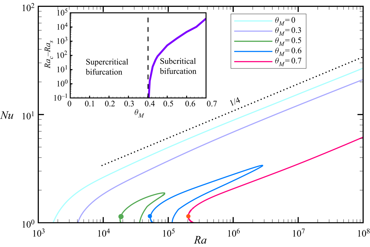
Once the Rayleigh number exceeds the critical value, the flow is unstable and steady convection cells will emerge. To obtain the exact non-trivial steady solutions when the flow is unstable, we added the critical mode onto the base state as the initial guess of the Newton iteration. By slightly moving away from the critical point predicted by the linear stability, convergence is fast when the amplitude of the eigenvector is well chosen. Typically, we used a bisectional method to choose the eigenvector's amplitude. Figure 2 illustrates the bifurcation diagram at $Pr=1$ for several different values of $\theta _M$ by fixing the domain width at $2{\rm \pi} /\alpha _c$. 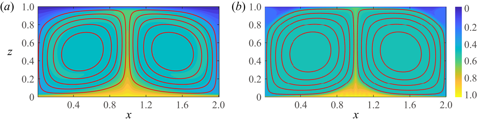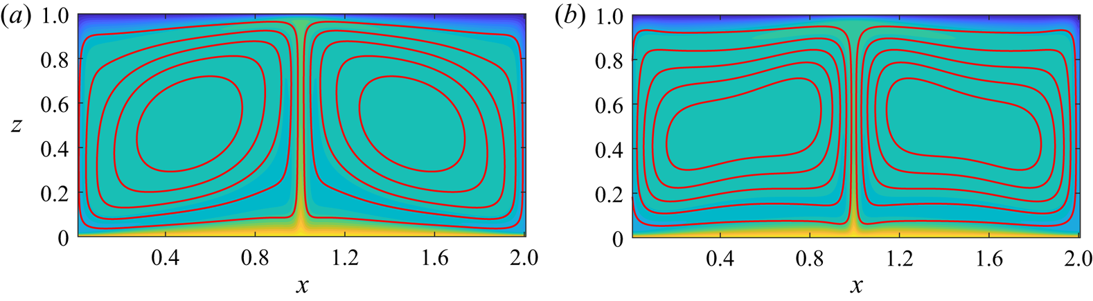An interesting observation is that the instability is supercritical when $\theta _M\lesssim 0.4$ but becomes subcritical as $\theta _M\gtrsim 0.4$. Figure 3 illustrates the flow field and the temperature field of the steady solution for two selected Rayleigh numbers $Ra=10^{6}, 10^{8}$ at $\theta _M=0$. 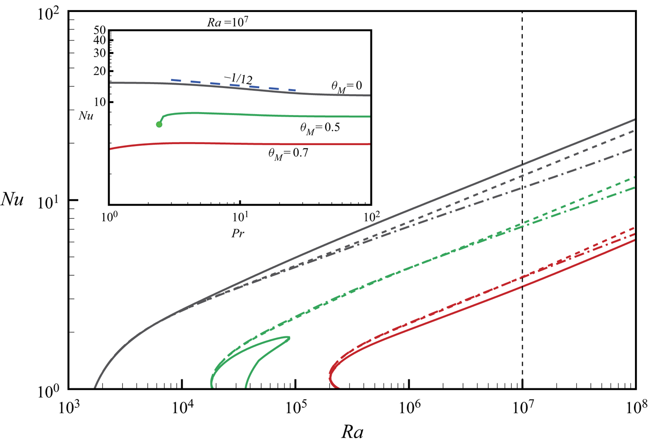The convection pattern is very similar to that in the classical Rayleigh–Bénard convection, in that the thickness of the plume in the centre (hot fluid around $x=0$) becomes thinner as $Ra$ increases and small-scale convection cells develop within the hot (cold) plumes near the bottom (top) plane (see also Wen et al. Reference Wen, Goluskin and Doering2020). However, the difference between penetrative convection and the classical Rayleigh–Bénard convection is that the hot/cold plumes are not centro-symmetric and the small-scale motions in the cold plumes are much weaker than that in the hot plumes. We also observe that the heat flux scales as $Ra^{1/4}$ at $\theta _M=0$ when the aspect ratio is fixed at $L\approx 2$, which is an additional similar feature as the classical Rayleigh–Bénard convection.

Figure 2.

The bifurcation diagram in the $Ra$–$Nu$ plane. The Prandtl number is fixed at $Pr=1$. In the inset, we show $Ra_c-Ra_s$ versus $\theta _M$, where $Ra_s$ is the minimal Rayleigh number on the $Nu$–$Ra$ curve as marked by bullets in the main panel. The subcritical bifurcation occurs when $\theta _M\gtrsim 0.4$. The domain width is fixed at $2{\rm \pi} /\alpha _c$ for each $\theta _M$.

Figure 3.

The flow field and temperature field at (a) $Ra=10^{6}$ and (b) $Ra=10^{8}$. The other parameters are $\theta _M=0$ and $Pr=1$. The red lines are the streamlines and the colour bar marks the contours of the temperature field, which applies to all the remaining figures of temperature field in this study.

To understand this similarity, we assume that the main viscous dissipation is in the boundary layer. Since the total viscous dissipation rate is proportional to $U^{3}/d$ (where $U$ is the bulk velocity), the total viscous dissipation rate is proportional to $Re^{3}$ (here $Re=Ud/\nu$ is the Reynolds number; see Grossmann & Lohse Reference Grossmann and Lohse2000). Because we consider $Pr=1$, the thickness of the velocity boundary layer is the same as the thermal boundary layer, which is proportional to $Re^{-1/2}$ (see p. 159 in Landau & Lifshitz Reference Landau and Lifshitz2004). Hence, the viscous dissipation rate in the boundary layer is proportional to $Re^{3}\times Re^{-1/2}=Re^{5/2}$, which should be balanced by the work done by buoyancy: $Ra\langle w\theta ^{2}\rangle =\langle \|\boldsymbol {\nabla }\boldsymbol {u}\|^{2}\rangle$. Hence, we have $Ra\langle w\theta ^{2}\rangle \sim Re^{5/2}$. Because $\langle w\theta ^{2}\rangle \sim \langle w\theta \rangle \sim Nu$ (see Appendix A) and $Re\sim Ra^{1/2}$ (see Grossmann & Lohse Reference Grossmann and Lohse2000), we have $Nu\sim Ra^{1/4}$. This scaling law persists when the bifurcation is supercritical, i.e. $\theta _M<0.4$, and an example of $\theta _M=0.3$ is shown in figure 2. Reference Toppaladoddi and WettlauferToppaladoddi & Wettlaufer's (Reference Toppaladoddi and Wettlaufer2018) direct numerical simulations suggest that $Nu$ scales slightly higher than $Ra^{1/4}$ when the thickness of the stably stratified layer at the base state is very thin (corresponding to $\theta _M=0$ in the present study), indicating that the steady solution at the fixed aspect ratio $L\approx 2$ is not the optimal case. When the thickness of the stable layer becomes thick, their numerical results show that $Nu$ scales like $Ra^{\gamma }$ (with $0.245<\gamma <0.287$) in the regime of $10^{6}\le Ra\le 10^{8}$, depending on the thickness of the stable layer.

When the thickness of the stable layer $\theta _M\gtrsim 0.4$, our study shows that the solution in the form of a single pair of steady convection cells does not exist if $Ra$ exceeds a certain value and the curve bends back and connects to the bifurcation branch of the solution in the form of two pairs of steady convection cells (e.g. see figure 2, $\theta _M=0.5,0.6$). The curve for $\theta _M=0.7$ also turns back at higher Rayleigh number, which is not shown here. In direct numerical simulations, Toppaladoddi & Wettlaufer (Reference Toppaladoddi and Wettlaufer2018) found unsteady solutions at high $Ra$ when the thickness of the stable layer is thick, suggesting that a Hopf bifurcation occurs when the steady solution becomes unstable.

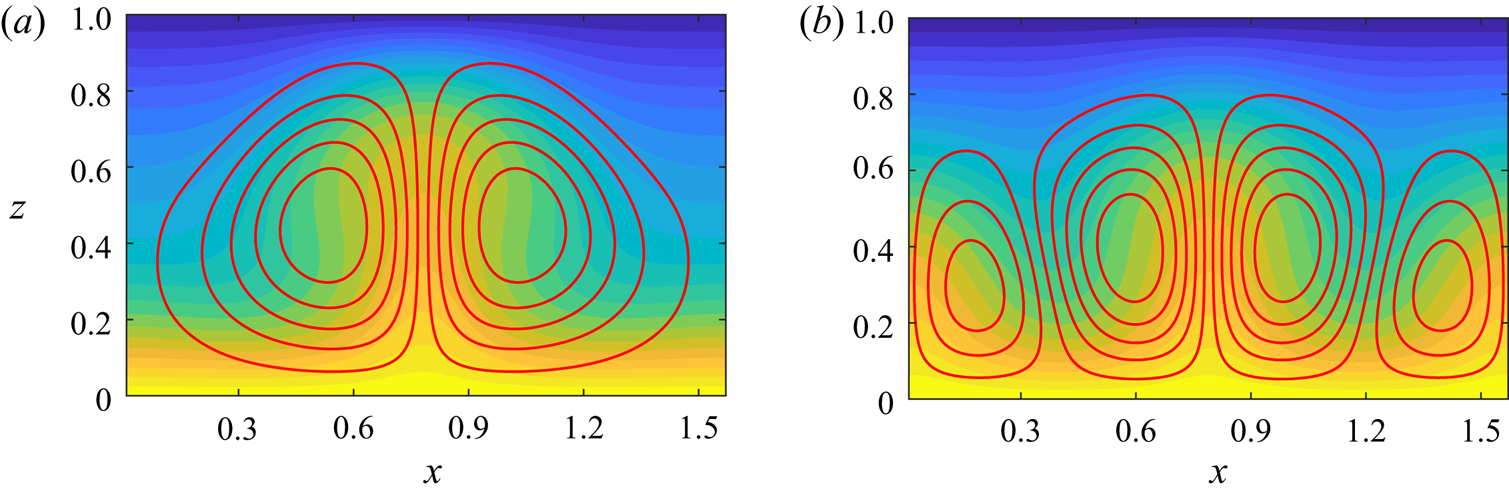
Figure 4 illustrates the two types of steady solutions at $\theta _M=0.5$. It shows that the solution with one pair of convection cells becomes distorted (but the two cells are the same size) and the convection cells in the solution with two pairs of convection cells are not the same size (the four cells are the same size at the bifurcation point). An implication of the results in figure 2 is that the solution in the form of one pair of convection cells can transport more heat. When the stable layer is thicker (e.g. 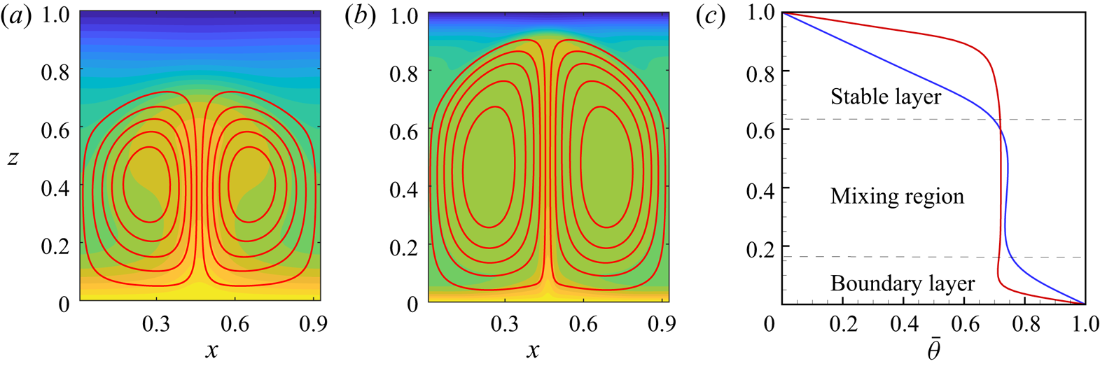$\theta _M=0.7$), a clear penetrative flow can be seen in figure 5(a,b), which shows that the convection initiated in the lower unstable layer is confined not only by the upper stably stratified layer but also by the upper rigid wall. It is therefore fascinating to investigate the asymptotic behaviour of $\theta _M\rightarrow 1^{-}$ and $Ra\rightarrow \infty$ in future. Note that the slope of the mean temperature field in the boundary layer is the same as that in the stable layer, which can be used to simply give an estimate of the thickness of the stable layer (denoted as $h$) when convection occurs at large $Ra$. Assuming that the power-law ansatz $\delta \sim Ra^{-\gamma }$ (with $\delta$ being the boundary layer thickness and $Nu\sim Ra^{\gamma }$), the thickness of the stably stratified top layer can be estimated by $h=\delta \theta _{mix}/(1-\theta _{mix})\sim {\theta _{mix}/(1-\theta _{mix})Ra^{-\gamma }}$, where $\theta _{mix}$ is the mean temperature in the mixing region. However, it is obvious that the scaling law does not hold for all $\theta _M$ since the steady solution does not always exist at large $Ra$ when $\theta _M>0.4$. But when $\theta _M<0.4$, the numerical data suggest $\gamma =1/4$ here.

Figure 4.

The flow field and temperature field at $Ra=50\,000$, with $Pr=1$ and $\theta _M=0.5$. (a) The upper branch solution and (b) the lower branch solution.

Figure 5.

The flow field and temperature field at (a) $Ra=10^{6}$ and (b) $Ra=10^{8}$. (c) The mean temperature field $\bar {\theta }$ of the two cases: blue line for $Ra=10^{6}$ and red line for $Ra=10^{8}$. The dashed lines are plotted to indicate three different regions at $Ra=10^{6}$. The other parameters are $\theta _M=0.7$ and $Pr=1$.

An interesting feature similar to the classical Rayleigh–Bénard convection is that the mean temperature profile in the boundary layer is non-monotonic (see figure 5c), which indicates that there is an unstably stratified layer in the boundary layer. The non-monotonic behaviour in the mean temperature profile is clearly dependent on $\theta _M$ and the Rayleigh number $Ra$ (in fact, it also depends on $Pr$). However, the temperature is monotonic in the stable top layer, which is a very different feature from the classical Rayleigh–Bénard convection. (In the classical Rayleigh–Bénard convection, there exist two unstably stratified layers: one in the bottom boundary layer and the other in the top boundary layer.) We also observe that the mean temperature profiles in figure 5(c) share many features as the direct numerical simulation by Toppaladoddi & Wettlaufer (Reference Toppaladoddi and Wettlaufer2018). The thickness of the bottom boundary layer becomes thinner as $Ra$ increases and the mixing temperature $\theta _{mix}$ is a bit higher than $\theta _M$, which is almost constant in the mixing region. However, the boundary layer by Toppaladoddi & Wettlaufer (Reference Toppaladoddi and Wettlaufer2018) is thinner than ours, indicating that the 2-D steady flow field could transfer less heat than a 2-D chaotic flow field when the aspect ratio is fixed at $2{\rm \pi} /\alpha _c$. The optimal domain size, in which steady solutions transfer more heat than chaotic solutions, will be explored in § 4.

Figure 6 illustrates the influence of Prandtl number $Pr$ on the steady solutions. Here, we considered $1\le Pr\le 100$ and the result shows that the heat transfer decreases as $Pr$ increases when $\theta _M$ is small. This is because the increased viscous effect retards the efficiency of heat transfer. For small $\theta _M$, i.e. the thickness of the stably stratified layer is thin (e.g. $\theta _M=0$), we also found that the scaling law of heat transfer $Nu\sim Ra^{\gamma }$ for the two values of Prandtl number $Pr=1,11.6$ is the same and $\gamma =1/4$, but $\gamma$ is clearly less than $1/4$ for $Pr=100$ (perhaps because $Ra$ is not high enough before the $1/4$ scaling emerges at large $Pr$). In the range of $2< Pr<30$, our numerical data suggest $Nu\sim Pr^{-1/12}$. To account for the influence of Prandtl number on the heat transfer, we rescale the viscous dissipation rate $\langle |\boldsymbol {\nabla }\boldsymbol {u}|^{2}\rangle$ in units of $\nu ^{3}/d^{4}$ (see Grossmann & Lohse Reference Grossmann and Lohse2000). Hence, we have $\langle |\boldsymbol {\nabla }\boldsymbol {u}|^{2}\rangle \sim Pr^{-2}Ra\langle w\theta ^{2}\rangle \sim Pr^{-2}RaNu$ (see Appendix A to see that $\langle w\theta ^{2}\rangle$ is linearly proportional to $Nu$). When $Pr>1$, the viscous boundary layer is thicker than the thermal boundary layer, and the heat transfer is proportional to $Re^{1/2} Pr^{1/3}$ (see Landau & Lifshitz Reference Landau and Lifshitz2004). Since the work done by buoyancy should be balanced by the viscous dissipation ($\sim Re^{5/2}$), we have $Nu\sim Ra^{1/4}Pr^{-1/12}$, which is supported by the numerical evidence in figure 6. However, the $Pr^{-1/12}$ scaling breaks down when $Pr$ is large (roughly $Pr>30$), and our numerical solution of the steady state suggests $Pr$ has a negligible influence on $Nu$, but the flow field is noticeably changed (see figure 7). The streamlines are more like a square pattern at high $Pr$, while the streamlines are tilted at small $Pr$. However, it has not been examined if $Nu\sim Pr^{-1/12}$ persists at large $Pr$ in turbulent flows, which requires future investigation.

Figure 6.

The bifurcation diagram in the $Ra$–$Nu$ plane: influence of Prandtl number. In the main panel, three different Prandtl numbers are considered: black, green and red solid lines for $Pr=1$; black, green and red dashed lines for $Pr=11.6$; and black, green and red dash-dotted lines for $Pr=100$. The different colours mark different values of $\theta _M=0, 0.5, 0.7$ (black, green and red, respectively). In the inset, the Rayleigh number is fixed at $Ra=10^{7}$ and three typical $\theta _M=0, 0.5, 0.7$ are considered.

Figure 7.

The flow field and temperature field at (a) $Pr=11.6$ and (b) $Pr=100$. The other parameters are $\theta _M=0$ and $Ra=10^{7}$.

For a thick stably stratified layer (e.g. $\theta _M=0.5, 0.7$), we observe that the heat transfer first increases as $Pr$ increases, and then it becomes invariant as $Pr$ increases to large numbers. For small $Pr$, the hot plume is too weak to penetrate into the top stably stratified layer so that the solution does not exist at high $Ra$. But when $Pr$ is large, figure 8(a,b) suggests that the hot plume can penetrate deeper into the top stably stratified layer, which causes the increase in heat transfer and steady solutions do exist at large $Ra$. This implies that the thickness of the thermal boundary layer plays an important role in the bifurcation scenario. For the same Rayleigh number, when the thermal boundary layer is thick ($Pr$ is small), it is more unstable and the two additional convection cells could develop due to the instability (for example, there are more convection cells in the numerical simulation by Toppaladoddi & Wettlaufer (Reference Toppaladoddi and Wettlaufer2018) at $Pr=1$). When the Prandtl number is large, the thermal boundary layer is relatively thinner than the viscous boundary layer and is more stable, which accounts for the existence of steady solutions in the form of one pair of convection cells at high $Ra$. When the Prandtl number is large, the numerical data show that the Prandtl number has a very weak influence on the steady solutions (see figure 8c,d). The $Ra^{1/4}$ scaling has also been observed by us for $\theta _M=0.5, 0.7$ at $Pr=11.6$ (this scaling law is not observed at $Pr=1$ for $\theta _M=0.5$ because steady solutions in the fixed domain of aspect ratio $2{\rm \pi} /\alpha _c$ do not exist at high $Ra$). The $Ra^{1/4}$ scaling seems to break down for $\theta _M=0.5, 0.7$ when $Pr=100$, which, perhaps, is also because $Ra$ is too low before the $1/4$ scaling can emerge. But an obvious difference is that the $Pr^{-1/12}$ scaling does not appear for the two cases $\theta _M=0.5, 0.7$. It is questionable whether the $Pr^{-1/12}$ scaling is observable in turbulent penetrative convection when $\theta _M>0.4$ by direct numerical simulations, which also needs further investigation.

Figure 8.

The flow field and temperature field at $Ra=10^{7}$ for: (a) $Pr=11.6$, $\theta _M=0.5$, $\alpha =4$; (b) $Pr=100$, $\theta _M=0.5$, $\alpha =4$; (c) $Pr=11.6$, $\theta _M=0.7$, $\alpha =6.78$; and (d) $Pr=100$, $\theta _M=0.7$, $\alpha =6.78$. The horizontal axis is rescaled to $\alpha x$.

4. Optimal heat transfer by steady solutions

In this section, we examine how the 2-D optimal steady solutions depend on $\theta _M$, $Ra$ and $Pr$. Particularly, we will examine the two cases $Pr=1, 11.6$ in detail, which have been investigated via direct numerical simulations by Toppaladoddi & Wettlaufer (Reference Toppaladoddi and Wettlaufer2018) and Wang et al. (Reference Wang, Zhou, Wan and Sun2019). The Prandtl number $11.6$ specifically corresponds to water around $T=4\,^{\circ } \text {C}$. The 2-D optimal solutions are tracked from the bifurcation point, i.e. aspect ratio $2{\rm \pi} /\alpha _c$, and by adjusting the aspect ratio (or the width of the convection cell, $L=2{\rm \pi} /\alpha$) at each Rayleigh number like Sondak et al. (Reference Sondak, Smith and Waleffe2015), Waleffe et al. (Reference Waleffe, Boonkasame and Smith2015) and Wen et al. (Reference Wen, Goluskin and Doering2020). We applied a pseudo-arclength continuation method to track the solutions and found that the optimal solution, indeed, can also be tracked from the cutoff wavenumber for each $Ra$, as demonstrated in figure 9.

Figure 9.

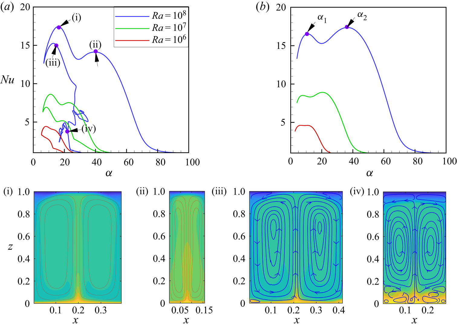
(a,b) The Nusselt number $Nu$ versus the base wavenumber $\alpha$ for: (a) $\theta _M=0.5$ and $Pr=1$; and (b) $\theta _M=0.5$ and $Pr=11.6$. Two local maxima in (b) are marked by points. Panels (i)–(iv) are flow fields and temperature fields at $Ra=10^{8}$ as marked in (a).

It is interesting that the topological structure of the $\alpha$–$Nu$ curve ($\alpha$ is the base wavenumber of the problem, $\alpha =2{\rm \pi} /L$) resembles a raven, and there are two local maxima on its head and back (the other local maxima on the belly are not important, so are not shown in figure 10), which are marked by points in figure 9(b). The other two cases $\theta _M=0, 0.7$ (see figure 10) also show that there are two local maxima when the Rayleigh number is large. The numerical data indicate that the optimal heat transfer is achieved at the small wavenumber $\alpha _1$ when $Pr<10$, but it is achieved at the large wavenumber $\alpha _2$ when $Pr>10$. This is a similar feature to the classical Rayleigh–Bénard convection (see Sondak et al. Reference Sondak, Smith and Waleffe2015). Figure 9(i,ii) shows that the flow field can penetrate the whole domain for both $\alpha =\alpha _1, \alpha _2$, which causes a much higher heat flux than the steady solutions in a fixed domain size ($L=2{\rm \pi} /\alpha _c$) in § 3.2. The steady solutions on the raven's belly show that there are multiple convection cells arrayed in the wall-normal direction (see figure 9iii,iv), which is less efficient to transfer heat. This indicates that the small-scale motion near the walls in penetrative convection does not really help to enhance heat transfer.

Figure 10.

The Nusselt number $Nu$ versus the base wavenumber $\alpha$ for: (a) $\theta _M=0$ and $Pr=1$; (b) $\theta _M=0$ and $Pr=11.6$; (c) $\theta _M=0.7$ and $Pr=1$; and (d) $\theta _M=0.7$ and $Pr=11.6$.

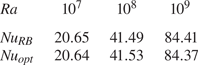
A comparison between the classical Rayleigh–Bénard convection and penetrative convection shows that the optimal heat transfer in penetrative convection at $\theta _M=0$ and $Pr=1$ is very close to the classical Rayleigh–Bénard convection (see table 2). But the optimal temperature field in the classical Rayleigh–Bénard convection obeys centro-reflection symmetry, while this symmetry is lost in penetrative convection. In classical Rayleigh–Bénard convection, Waleffe et al. (Reference Waleffe, Boonkasame and Smith2015) and Wen et al. (Reference Wen, Goluskin and Doering2020) showed that the 2-D optimal flow field can transfer more heat than 3-D turbulent flow fields. In turbulent penetrative convection, there are many small-scale motions near the walls (see Wang et al. Reference Wang, Zhou, Wan and Sun2019), which is similar to the steady solutions in figure 9(iv). This might imply that turbulence is less efficient than the optimal steady solution for heat transfer. For example, direct numerical simulation of a 3-D turbulent penetrative convection at $(\theta _M, Ra)=(0.5, 10^{8})$ shows that the turbulent flow field can achieve $Nu=16.29$ (this Nusselt number was computed at $q=2$ by Dr Q. Wang in a cubic box of size $x\times y\times z =[-2,2]\times [-2,2]\times [0,1]$), which is approximately $10\,\%$ lower than the present 2-D optimal heat transfer $Nu=17.37$. Table 3 demonstrates that the heat flux in our 2-D optimal steady solution is higher than that in a 3-D turbulent flow at $q=2$, providing strong evidence that the 2-D optimal steady flow is more efficient to transport heat than a turbulent flow. But, as $\theta _M$ increases, the gap between the 2-D optimal heat flux and the 3-D turbulent heat flux narrows.

Table 2.

Comparison between the classical Rayleigh–Bénard convection and penetrative convection at $\theta _M=0$ and $Pr=1$. Here $Nu_{RB}$ (data courtesy of Dr B. Wen) and $Nu_{opt}$ are the optimal Nusselt numbers in the classical Rayleigh–Bénard convection and penetrative convection.

Table 3.

Comparison between the present study and the 3-D simulations. The 3-D simulations were performed in an $x\times y\times z=[-2,2]\times [-2,2]\times [0,1]$ box. The Prandtl number is $Pr=11.6$. Here $Nu^{*}$ is the Nusselt number obtained by 3-D direct numerical simulations (data courtesy of Dr Q. Wang); and $Nu_{opt}$ is the optimal Nusselt number in the present study.

Figure 11 shows how the optimal wavenumber $\alpha _{opt}$ (the wavenumber corresponding to the global maximal heat flux) depends on the Rayleigh number $Ra$. For $Pr=1$, the best fitting shows that the optimal wavenumber $\alpha _{opt}=\alpha _1$ scales like $Ra^{1/5}$. When $\theta _M=0.5, 0.7$, the $1/5$ scaling of the optimal wavenumber seems to connect with the primary instability $\alpha _c\sim Ra^{1/5}$. When $\theta _M=0$, the argument for $\alpha _c\sim Ra^{1/5}$ breaks down (see (3.2)). Thus, it seems that $1/5$ scaling of the optimal wavenumber is connected with the primary instability as $\theta _M\rightarrow 0^{+}$. For $Pr=11.6$, the best fitting shows that the optimal wavenumber $\alpha _{opt}=\alpha _2$ scales like $Ra^{1/4}$, which is connected to the cutoff wavenumber like the classical Rayleigh–Bénard convection (Sondak et al. Reference Sondak, Smith and Waleffe2015). The present study also suggests that the power exponent for the optimal wavenumber $\alpha _{opt}=\alpha _2$ is not sensitive to the thickness of the stably stratified top layer. To understand the physics, using the exchange of stability (Veronis Reference Veronis1963), we can obtain a sixth-order equation for the linear stability of a small disturbance $\theta ^{\prime }=\hat {\theta }(z)\exp (\omega t+\textrm {i}\alpha x)$ (for neutral instability $\omega \equiv 0$):

(4.1)\begin{equation} (\text{D}^{2}-\alpha^{2})^{3}\hat{\theta}+2\alpha^{2}Ra(1-z-\theta_M)\hat{\theta}=0,\quad \text{D}:=\frac{\textrm{d}}{\textrm{d}z}. \end{equation}

Here, we treat $\alpha$ as the eigenvalue but $Ra$ is given. It requires that $\alpha ^{6}\hat {\theta }\sim \alpha ^{2} Ra(1-z-\theta _M)\hat {\theta }$ (this is because $\alpha$ is large and the horizontal diffusive term should dominate the wall-normal diffusive term). Hence, we obtain that the cutoff wavenumber scales as $\alpha \sim Ra^{1/4}$, and decreases as $\theta _M$ increases.

Figure 11.

The optimal base wavenumber number $\alpha$ versus the Rayleigh number $Ra$. The hollow symbols are for $\alpha _2$ and solid symbols are for $\alpha _1$. Lines are obtained using best fitting.

The 2-D optimal heat flux characterized by $Nu$ versus Rayleigh number $Ra$ is shown in figure 12. For $Ra\rightarrow \infty$, we derived an upper bound on the heat flux: $Nu\sim Ra^{1/2}$ (see Appendix A), which is uniform in $Pr$. However, in our derived upper bound $Nu\lesssim cRa^{1/2}$, it shows that the power exponent is independent of $\theta _M$, i.e. the thickness of the stably stratified top layer. But the undetermined coefficient $c$ depends on $\theta _M$. It is interesting that the power exponent of the bound on heat flux in penetrative convection is the same as that in the classical Rayleigh–Bénard convection ($Nu\lesssim 0.026Ra^{1/2}$; Plasting & Kerswell Reference Plasting and Kerswell2003). However, as discussed in Ding & Kerswell (Reference Ding and Kerswell2020), the upper bound is not observable because there is no field satisfying the momentum and energy equations. This does not mean that the $Ra^{1/2}$ scaling (usually referred to as the ultimate scaling in classical Rayleigh–Bénard convection) is wrong at very large $Ra$, but their analysis suggested that any true scaling should be lower than the bound. It is clear that the optimal solution is much lower than the bound and the power index $\gamma$ (power-law ansatz $Nu\sim Ra^{\gamma }$) is less than $1/2$, which seems to be consistent with the scaling proposed by Veronis (Reference Veronis1963): $Nu\sim Ra^{1/3}$ when $Ra<10^{9}$. The $Ra^{1/3}$ scaling can be derived under a marginal stable boundary layer assumption. Suppose that the thickness of the boundary layer is $\delta$ and the temperature in the mixing region is $\theta _{mix}$, then $Nu=(1-\theta _{mix})\delta ^{-1}$. The thickness of a marginally stable boundary layer is proportional to $\delta /d\sim (1-\theta _{mix})^{-2/3}Ra^{-1/3}$ (this also gives a scaling for the thickness of the stably stratified top layer $h\sim Ra^{-1/3}$).

Figure 12.

The optimal Nusselt number $Nu-1$ versus the Rayleigh number $Ra$. The slope $1/2$ indicates the upper bound on the heat transfer $Nu\le cRa^{1/2}$. Lines are obtained using best fitting. See also symbols in figure 11.

Figure 13 displays three typical mean temperature profiles $\bar \theta$ at $Ra=10^{8}$, which clearly demonstrate that there is a laminar thermal boundary layer near the bottom wall. And, as $\theta _M$ increases, the boundary layer is thicker, and the mean temperature in the mixing region $\theta _{mix}$ is higher. We further assume that $\theta _{mix}$ is linearly dependent on $\theta _M$ as $\theta _{mix}=1-c+c\theta _M$ (Reference Wang, Zhou, Wan and SunWang et al.'s (Reference Wang, Zhou, Wan and Sun2019) data suggest this linear relationship for fixed Prandtl number), thus $\delta /d\sim (1-\theta _M)^{-2/3}Ra^{-1/3}$. Hence, the heat flux scales like $Nu\sim (1-\theta _M)^{5/3}Ra^{1/3}$. Numerical data at $Ra=10^{8}$ give $Nu_{opt}=35.85, 17.37, 7.78$ for $\theta _M=0, 0.5, 0.7$ when $Pr=11.6$, which roughly reduces by a factor of $(1-\theta _M)^{5/3}$. For $\theta _M=0$, the scaling is very much like the classical Rayleigh–Bénard convection in which $\gamma \approx 0.31$ (Sondak et al. Reference Sondak, Smith and Waleffe2015; Waleffe et al. Reference Waleffe, Boonkasame and Smith2015; Motoki et al. Reference Motoki, Kawahara and Shimizu2020). For the other two cases of $\theta _M=0.5, 0.7$, the power exponent $\gamma \approx 0.328, 0.339$, which are all higher than the 2-D or 3-D direct numerical simulations (Toppaladoddi & Wettlaufer Reference Toppaladoddi and Wettlaufer2018; Wang et al. Reference Wang, Zhou, Wan and Sun2019). It is worth noting that the power exponent for $\theta _M=0.7$ is $\gamma =0.339$ and is higher than $1/3$, which does not indicate that the flow has entered into the ultimate regime. It is because the Rayleigh number is not high enough and the scaling is not clear when $Ra<10^{9}$ for a thick stably stratified top layer (see the data fitting in the range of $10^{8}\le Ra\le 5.623\times 10^{9}$ in Appendix B). We would expect that $\gamma <1/3$ or asymptotically approaches $1/3$ at very large $Ra$ like the classical Rayleigh–Bénard convection (Wen et al. Reference Wen, Goluskin and Doering2020). But it is not known if heat transfer by unsteady flow fields can be higher than $Ra^{1/3}$ scaling but below the upper bound $Ra^{1/2}$, which remains a challenging problem.

Figure 13.

The horizontal averaged temperature profile $\bar \theta$ for the optimal steady solutions at $Ra=10^{8}$ and $Pr=11.6$.

The mean temperature profiles in figure 14 confirm that the thickness of the thermal boundary layer is thick at small Prandtl number but is thin at large Prandtl number. For $Pr>10$, we found that the Prandtl number has a negligible influence on the mean temperature profile, but the mean temperature profile at small Prandtl number is significantly different from that at large Prandtl number. The mean temperature in the mixing region is lower for small Prandtl numbers, as seen in figure 14. To understand the underlying physics, we refer to figure 9. For small Prandtl number, the optimal temperature field in figure 9(i) shows that a hot plume penetrates into the fluid layer with two arm-like structures near the top wall. For large Prandtl numbers, the optimal temperature field is like figure 9(ii) and has no significant horizontal structures. The optimal convection is very vigorous in a narrow domain and more of the cold fluid can be heated up by the central hot plume when the Prandtl number is large. Hence, the mean temperature in the mixing region for $Pr>10$ is higher than the mean temperature in the mixing region for $Pr<10$.

Figure 14.

The horizontal averaged temperature profile $\bar \theta$ at $Ra=10^{8}$ and $\theta _M=0.5$.

The influence of the Prandtl number on the optimal solution is examined over three decades, $10^{-1}\le Pr\le 10^{2}$, and the results are illustrated in figure 15. For $\theta _M=0$, $Nu$ decreases with $Pr$ when $Pr$ is small, and then it becomes invariant when $Pr$ is large. For $\theta _M=0.5, 0.7$, however, we observed that $Nu$ slightly increases with $Pr$ when $Pr<1$, and $Nu$ becomes invariant when $Pr>1$. For $\theta _M=0$, the behaviour $Nu\sim Pr^{-1/12}$ is observed again when $1\le Pr\le 10$. Hence, we propose that $Nu\sim Pr^{-1/12}Ra^{1/3}$ in this regime ($1< Pr<10$) for $\theta _M=0$. Such a phenomenon is different from the classical Rayleigh–Bénard convection, in which $Nu$ was reported to be very weakly dependent on $Pr$ (Sondak et al. Reference Sondak, Smith and Waleffe2015). However, $Nu$ becomes independent of $Pr$ when $Pr>10$, which is similar to the classical Rayleigh–Bénard convection. This suggests that, for $Pr>1$, the Nusselt number does not simply follow $Nu\sim Re^{1/2}Pr^{1/3}$ and the viscous dissipation is not simply proportional to $Re^{5/2}$. When $Pr<1$, if the viscous dissipation is dominated by the viscous boundary layer and $Nu\sim Re^{1/2}Pr^{1/2}$ (the Grossmann & Lohse (Reference Grossmann and Lohse2000) theory for $Pr<1$), we obtain $Nu\sim Ra^{1/4}Pr^{1/8}$, which is rejected immediately by the data of $\theta _M=0$. Although our data for $\theta _M=0.5, 0.7$ show that $Nu$ increases with $Pr$ when $Pr<1$, it does not support the $Ra^{1/4}Pr^{1/8}$ scaling. This suggests that the Grossmann & Lohse (Reference Grossmann and Lohse2000) theory for the classical Rayleigh–Bénard convection is clearly inapplicable for the 2-D steady optimal solutions in penetrative convection.

Figure 15.

The optimal Nusselt number $Nu$ versus the Prandtl number $Pr$ at $Ra=10^{8}$. Circles are for $\theta _M=0$, triangles are for $\theta _M=0.5$ and diamonds are for $\theta _M=0.7$.