



Nomenclature
- b
-
bias
- C
-
penalty parameter
- CFD
-
computational fluid dynamics
- CNN
-
convolutional neural network
- c
-
memory cell
- D
-
dataset
- D left
-
datasets obtained after splitting the dataset D
- D right
-
datasets obtained after splitting the dataset D
- |D|
-
number of samples in the dataset D
- GPR
-
Gaussian process regression
- h
-
hidden state
- K
-
convolution kernel
- k(x, x ′)
-
kernel function
- LE
-
leading edge
- LSTM
-
long short-term memory network
- l
-
length scale
- MAE
-
mean absolute error
- MLP
-
multi-layer perceptron
- ML
-
machine learning
- MRE Int
-
mean relative error relative to the interval length
- MSE
-
mean square error
- m(x)
-
mean function
-
 $p^{*}_{\textit{1}}$
-
stator inlet total pressure
-
$p^{*}_{\textit{2}}$
-
stator outlet total pressure
- RBF
-
radial basis function
- RF
-
random forest
- RMSE
-
root mean square error
- R 2
-
coefficient of determination
- R 1_in
-
slot inlet radial position close to the casing
- R 1_out
-
slot outlet radial position close to the casing
- R 2_in
-
slot inlet radial position close to the hub
- R 2_out
-
slot outlet radial position close to the hub
- SHAP
-
shapley additive explanation
- SVR
-
support vector regression
- TE
-
trailing edge
- t
-
time
- Var
-
total variance
- W in
-
slot inlet width
- W out
-
slot outlet width
- w
-
weight
- X i
-
a sample
- X *
-
samples that need to be predicted by Gaussian process regression
- x i
-
input of the i-th neuron
- y j
-
output of the j-th neuron
- y *
-
prediction result
- y true
-
true value (in this study, referring to CFD numerical values)
-
$\overline {{y_{\textit{true}}}} $
-
average value of the true values
- y true,max
-
maximum value of the true values
- y true,min
-
minimum value of the true values.
- Z in
-
slot inlet axial position
- Z out
-
slot outlet axial position
- Z 1_in
-
slot inlet axial position close to the leading edge
- Z 1_out
-
slot outlet axial position close to the leading edge
- Z 2_in
-
slot inlet axial position close to the trailing edge
- Z 2_out
-
slot outlet axial position close to the trailing edge
- Z l
-
result of the convolution calculation in Step l
- ∑*
-
uncertainty of the predicted value
- 1D-CNN
-
one-dimensional convolutional neural network


Greek symbol
- α i
-
Lagrange function multiplier
-
$ \alpha^{*}_i $
-
Lagrange function multiplier
- ɛ
-
noise
- ξ
-
errors interval or insensitive band
-
$\xi ^{\wedge}_i $
-
upper boundary slack variables
-
$\xi ^{\vee}_i $
-
lower boundary slack variables
-
$\eta$
DE
-
compressor design point efficiency
- λ i
-
lagrange function multiplier
-
$\lambda ^{*}_i$
-
lagrange function multiplier
- μ *
-
predicted value of Gaussian process regression
- σ
-
standard deviation
- σ(x)
-
activation function
- σ *
-
stator total pressure recovery coefficient
-
$\sigma ^2_{f}$
-
signal variance
-
$\sigma ^2_{n}$
-
variance of noise
-
$\sigma ^2_{NS}$
-
stator total pressure recovery coefficient at the near-stall point


1.0 Introduction
The design of compressors is evolving towards higher loading and higher single-stage pressure ratio. However, under off-design operating conditions, the internal flow in compressors is often accompanied by significant flow losses, which not only lead to a notable decrease in compressor efficiency [Reference Dickens and Day1] but may also threaten its aerodynamic stability [Reference Liu, Chu, Zhang and Wang2–Reference Wang, Zhang, Chu and Jing8]. Employing appropriate flow control strategies is expected to address this challenge. Compared with active flow control strategies, passive flow control strategies do not require additional energy input and are more widely applied. As a passive flow control strategy, slotted blade technology [Reference Wang, Zhang, Jing, Feng and Xiao9, Reference Wang, Zhang, Guo, Li and Chu10] can effectively suppress boundary layer separation and reduce flow losses. Its basic principle is to utilise the pressure difference between the suction and pressure surfaces of the blade to form a slot-jet, thereby energising the low-energy fluid and minimising flow losses.
Since Rockenbach et al. [Reference Rockenbach11] first applied slotted blade technology to the compressor internal flow control, significant research efforts have been devoted to understanding its underlying physical mechanisms and optimising its design. The fundamental benefit of slotted blades stems from the slot-jet’s ability to suppress boundary layer separation. Over time, several consensus points have emerged regarding how key geometric parameters influence the compressor performance:
Axial Position: The axial position where the slot-jet interacts with the boundary layer is critical. Mikolajczak et al. [Reference Mikolajczak, Weingold and Nikkanen12] emphasised that the slot’s effectiveness largely depends on its axial position. This was further refined by Mu et al. [Reference Mu and Lu13], whose numerical simulations demonstrated that the closer the slot outlet is to the separation point, the more obvious the improvement effect. This establishes a clear physical guideline: the slot outlet must be positioned to intervene precisely where the boundary layer is most susceptible to separation.
Slot Size and Mass Flow: The slot size directly governs the slot-jet energy. Zhou et al. [Reference Zhou, Wang, Zeng and Zhao14] investigated slots with different widths and found that an optimal slot width exists. A slot that is too narrow provides insufficient momentum to effectively control the boundary layer separation, while one that is too wide introduces excessive mixing losses at the slot outlet. This highlights the fundamental physical trade-off between achieving control benefits and minimising induced losses.
Radial Layout and Targeting: As corner separation is a primary source of loss in compressors, the radial positioning of the slot determines its ‘targeting’ effectiveness. Chen et al. [Reference Chen, Chen and Feng15] showed that combined slot schemes achieve better flow control across the entire blade span. A pivotal finding by Tang et al. [Reference Tang, Liu and Lu16] indicated that end-region slots are more effective than full-span slots, as the latter introduce unnecessary losses in mid-span regions where control is not needed. This underscores the physical principle of concentrating control energy in critical flow regions, such as the end-walls, where secondary flows and corner separation dominate.
Internal Slot Shape: Beyond basic parameters, the internal geometry of the slot itself influences performance. Studies on advanced configurations, such as the SC-type slot by Wang et al. [Reference Wang, Liu and Zhang17] and the shark-gill-inspired slot by Yang et al. [Reference Yang, Han and Zhong18], aim to reduce internal flow losses and optimise the direction and quality of the slot-jet. This represents a pursuit of refined performance by aligning the slot’s internal flow path with the desired aerodynamic outcome.
Despite these valuable insights into the physical mechanisms, the development and application of slotted blade technology face several persistent challenges in the design process:
-
1. Lack of a rapid and general modeling method: A fast and universal parametric three-dimensional modeling method for the slotted blade technology has not been established, hindering systematic exploration of the design space.
-
2. Reliance on inefficient trial-and-error approaches: The design process often gets trapped in the iterative cycle of Design-Experiment-Design, leading to long development cycles and low efficiency, especially when dealing with multiple interacting compressor aerodynamic parameters.
-
3. Comprehensive consideration of design and off-design points: The design of slotted blades often prioritises performance improvement under a single operating condition, lacking comprehensive consideration of its impact on the other working conditions.
Concurrently, machine learning (ML) has emerged as a powerful paradigm in fluid mechanics [Reference Tang, Zhu, Xiang, He, Zhao, Wang, Qian and Yuan19], demonstrating remarkable capabilities in establishing complex mapping relationships from data. ML models have been successfully applied for rapid flow field prediction [Reference Jin, Cheng, Chen and Li20–Reference Blechschmidt and Mimic22], performance inference from limited data [Reference Kong, Chang, Li and Li23, Reference Post, Winhart and di Mare24] and even optimising turbomachinery components [Reference Wang, Yang and Huang25–Reference Wu, Ba, Du, Zhang, Fan and Xu27]. However, the application of ML to guide the design and analysis of internal flow control strategies in compressors, particularly for the slotted blade technology, remains relatively scarce. The research on prediction models that directly link slotted blade parameters to comprehensive compressor aerodynamic performance is extremely limited.
Based on the above research background, this study innovatively introduces ML technology into the slotted blade technology, and constructs mapping relationships between the design parameters of slotted blade and the compressor aerodynamic parameters using computational fluid dynamics (CFD) simulation data. The prediction accuracy of six ML models, including one-dimensional convolutional neural network (1D-CNN), random forest (RF), support vector regression (SVR), Gaussian process regression (GPR), multi-layer perceptron (MLP) and long short-term memory network (LSTM), is evaluated, and finally the optimal prediction model is selected. This data-driven prediction model is able to effectively replace the traditional CFD method, reducing computational time to 0.89% of the original. It not only overcomes the technical bottleneck caused by the low efficiency of the traditional Design-Experiment-Design iterative method, but also provides key technical references for the intelligent design of the slotted blade.
2.0 A general and rapid three-dimensional design method for the slotted blade technology
Since Rockenbach [Reference Rockenbach11] first applied the slotted blade technology to the field of compressor internal flow control, the slotted blade technology has undergone an evolution from experimental verification and flow control mechanism exploration to parametric research. However, a three-dimensional slotted blade design method has yet to be established. Therefore, this study innovatively proposes a fast and universal three-dimensional design method for the slotted blade technology based on the suction and pressure surface parameters. This method enables slot modeling completion within 1 s, and its generality is manifested in its applicability to any cascade, as well as compressor rotors and stators. Figure 1 presents the flow chart of the three-dimensional slotted blade design method, with the specific steps outlined as follows:
Design parameters required for the three-dimensional slot modeling

Flow chart of the three-dimensional slotted blade design method.

Figure 1 Long description
The flow chart depicts the process of the three-dimensional slotted blade design method. It begins with Step 1, showing a plane with coordinates and a yellow quadrilateral labeled A, B, C, and D. Step 2 maps this quadrilateral onto a grid with specific coordinates and labels. Step 3 further refines the grid into smaller sections labeled 1 through 4. Step 4 shows the transformed plane with the refined grid applied back to the original coordinate system. Step 5 illustrates the final structure with labeled sections PS and SS, indicating the completion of the design process.
Step 1: Prepare the geometric models of the pressure and suction surfaces of the research object (cascade or compressor blade), and rotationally project them onto the (R, 0, Z) plane within the cylindrical coordinate system.
Step 2: Assign values to the parameters required for three-dimensional slot modeling within the normalised interval [0, 1] based on design experience or random sampling, and generate straight lines in the normalised region using these design parameters. The parameters required for three-dimensional slot modeling are listed in Table 1.
Specifically, taking the pressure surface as an example, for given values of R 1_in, R 2_in, Z 1_in and Z 2_in, four straight lines (R = R 1_in, R = R 1_in, Z = Z 1_in and Z = Z 2_in) can be generated within the normalised region. These lines intersect the boundary of the normalised region at points a *, b *, c *, d *, e *, f *, g * and h * in sequence.
Step 3: Map the straight lines obtained in Step 2 onto the projections of the suction or pressure surface on the (R, 0, Z) plane within the cylindrical coordinate system.
The specific approach involves mapping points a *, b *, c *, d *, e *, f *, g * and h *, resulting in points a, b, c, d, e, f, g and h. Taking point a * as an example, the mathematical relationship between point a * (Z 1_in, 1) and point a (Za, R a ) during mapping is expressed as:
 \begin{align}{Z_a} &= {Z_A} + {\rm{ }}({Z_B} - {Z_A}){\rm{ }} \times {Z_{1\_in}} \end{align}
 \begin{align}{R_a} &= {f_{AB}}({Z_a})\end{align}
where f AB denotes the mathematical expression that describes the geometric profile of line AB, obtained through sixth-order polynomial fitting. This is because the projection of any edge of the pressure surface onto the (R, 0, Z) plane within the cylindrical coordinate system is non-linear.
Step 4: Rotationally project the mapped straight lines onto the suction and pressure surfaces. The enclosed regions form the slot inlet and outlet, with the remaining region correspond to the solid part of the blade.
Step 5: Use straight lines as the internal geometry to connect the inlet and outlet contours of the slot to complete the modeling.
3.0 Construction and evaluation of prediction model
3.1 Database establishment
In this study, eight slot design parameters were selected as inputs, while two compressor aerodynamic parameters – namely, the compressor design point efficiency (
 $\eta$
DE
) and the stator total pressure recovery coefficient at the near-stall point (
 $\sigma ^2_{NS}$
) – served as outputs. The objective was to establish a mapping relationship between the design parameters and the compressor aerodynamic performance. In investigations involving slotted blades, the geometric characteristics of the slot are typically defined by the axial positions and widths of the slot inlet and outlet. Accordingly, the design parameters listed in Table 1 were converted into those in Table 2.
Parameters that need to be converted and their calculation methods

The passive flow control strategy seldom results in significant improvement in compressor performance at the design point [Reference Wang, Wu, Huang and Wang28]. Therefore, when designing slotted blade configurations, a key challenge often addressed is how to enhance compressor performance at other operating points while maintaining a satisfactory
 $\eta$
DE
. The total pressure recovery coefficient (σ
*) serves as an important parameter for evaluating stator performance, reflecting the extent of total pressure loss across the stator blade passage. It is defined by Equation (3):
 \begin{align}{\sigma ^*} = {{p_2^*} \mathord{\left/ {\vphantom {{p_2^*} {p_1^*}}} \right. } {p_1^*}}\end{align}
where
 $p ^*_{1}$
and
 $p ^*_{2}$
represent the total pressure at stator inlet and outlet.
Both
 $\eta$
DE
and
 $\sigma ^*_{NS}$
were taken into consideration to comprehensively capture the influence of the slotted blade on the compressor performance. Consequently, the mapping relationship between the design parameters and the aerodynamic performance can be formulated as follows:
 \begin{align}[{\eta _{DE}},\sigma _{NS}^*] = f[{Z_{in}},{W_{in}},{R_{1\_in}},{R_{2\_in}},{Z_{out}},{W_{out}},{R_{1\_out}},{R_{2\_out}}]\end{align}
To ensure that each design parameter conformed to a Gaussian distribution, the Latin hypercube sampling method was employed to generate the design parameters. A total of 1,508 datasets were obtained through numerical simulation. Prior to training the prediction model, the data were normalised and cleaned using the 3σ method. This process resulted in a final database comprising 1,489 samples. During model training, the data were split into training and test sets in an 8:2 ratio.
3.2 Description of ML methods
3.2.1 One-dimensional convolutional neural network (1D-CNN)
The 1D-CNN, a variant of CNN, is specifically designed for processing one-dimensional sequential data. As illustrated in Fig. 2, the model employs input padding prior to convolution to preserve the data dimension through the convolutional layers. Within each convolutional layer, operations of convolution, activation and pooling are integrated. Stacking multiple such layers enables the model to extract increasingly complex features. For the convolution kernel K = [k 1 , k 2 , k 3 ] and the sample X i , when it slides gradually with a stride of 1, the result Z l of the convolution calculation at the lth step is:
 \begin{align}{Z_l} = \sum\limits_{j = 1}^3 {({x_i}_{,(l + (j - 1))} \times {k_j})} \end{align}
Hyperparameters of the 1D-CNN model

Table 3 Long description
The table presents the hyperparameters of a 1D-CNN model. It consists of two columns labeled 'Parameter' and 'Value', and eight rows. The parameters include the number of convolution layers, size of convolution kernel, convolution stride, number of convolution channels, pooling type, size of the pooling kernel, number of fully connected layers, number of neurons, dropout rate, activation function, and loss function. The values for these parameters are two, three, one, 128/256, max pooling, two, three, 1024/256/64, 0.1, ReLU, and mean square error respectively.
Schematic of the 1D-CNN model.

Figure 2 Long description
The schematic illustrates the structure of a one-dimensional convolutional neural network (1D-CNN) model. The process begins with the input layer, which consists of multiple colored blocks. These inputs are passed through the first convolution layer, where a convolution kernel processes the data, followed by an activation function using ReLU and a max pooling operation. The output from the first convolution layer is then fed into the second convolution layer, which repeats the convolution, activation, and pooling steps. The processed data from the second convolution layer is then passed to a fully connected layer, depicted as a network of interconnected nodes. Finally, the fully connected layer outputs the results to the output layer, represented by a series of circles.
Following the convolution operation, a non-linear activation function σ(x) is applied to the result. Common activation functions include ReLU, Sigmoid and Tanh. The activated output then undergoes pooling, such as average or max pooling, for dimensionality reduction. Finally, a fully connected layer integrates these pooled local features into a global representation.
Suppose that the fully connected layer has m input neurons and n output neurons, the output value of output neuron j is
 ${y_j} = \sigma (\sum\limits_{i = 1}^m {({w_{ij}}{x_i} + {b_j})} )$
, where x
i
is the output of input neuron i, w
ij
is the weight connecting the input neuron i and the output neuron j, b
j
is the bias of the output neuron j. Table 3 presents the hyperparameters of the 1D-CNN model determined by grid search. The learning curves of the 1D-CNN model are presented in Appendix A.
3.2.2 Random forest (RF)
RF is an ensemble learning method that operates by constructing a multitude of decision trees and aggregating their predictions for regression or classification tasks. This ensemble mechanism confers strong resistance to overfitting and leads to superior generalisation performance.
Figure 3 shows the schematic of the RF model. The RF model is composed of n independent decision trees, and a subset of the training set data is randomly sampled to construct each decision tree. For any decision tree, a subset of the features is selected for node splitting, and the node splitting uses the minimisation of the variance of the sample set after splitting as the core criterion. That is, when the decision tree splits the dataset D into D left and D right , the goal is to minimise the total variance (Var) of the split datasets, and the definition of Var is given by Equation (6):
 \begin{align}Var = \frac{{|{D_{left}}|}}{{|D|}}Var({D_{left}}) + \frac{{|{D_{right}}|}}{{|D|}}Var({D_{right}})\end{align}
where |D|, |D
left
| and |D
right
| represent the number of samples corresponding to the dataset; Var(D
left
) and Var(D
right
) represent the variance corresponding to the dataset. The decision tree stops splitting when the number of samples falls below the minimum required for splitting or when the maximum depth of the tree is reached. Finally, the prediction results (
 $ y^{*}_{i} $
) of the individual decision trees aggregate to yield the final prediction result (y
*) of the RF, as shown in Equation (7). Table 4 presents the hyperparameters of the RF model determined by grid search.
 \begin{align}{y^*} = \frac{1}{n}\sum\limits_{i = 1}^n {y_i^*} \end{align}
Hyperparameters of the RF model

Schematic of the RF model.

Figure 3 Long description
The image presents a schematic diagram illustrating the random forest model employed in the study of slotted blade technology for compressors. The diagram shows a dataset being processed through multiple decision trees, each producing individual results. These results are then averaged to produce a final result. The decision trees are depicted as hierarchical structures with nodes and branches, indicating the decision-making process within the model. The image highlights the innovative approach of using machine learning to establish mapping relationships between design parameters and key aerodynamic performances, such as compressor design point efficiency and stator total pressure recovery coefficient at the near-stall point.
3.2.3 Support vector regression (SVR)
SVR is an extension of the support vector machine (SVM) for regression problems. When addressing regression tasks, SVR allows for errors within an insensitive region ξ. When the difference between the predicted value and the true value is less than ξ, it is considered that the prediction is accurate, where ξ is called the insensitive band. The goal of SVR is to find a function
 $f(x) = {w^T}x + b$
such that as much training data as possible falls in the ξ insensitive band and
 $||w||_2^2$
is as small as possible. The mathematical expression of SVR is:
 \begin{align}\begin{array}{l}{\min _{w,b,{\xi ^ \wedge },{\xi ^ \vee }}}\dfrac{1}{2}||w|{|^2} + C\sum\limits_{i = 1}^n {(\xi _i^ \wedge + \xi _i^ \vee )} \\[11pt]s.t.\left\{ {\begin{array}{*{20}{c}}{{y_i} - ({w^T}{x_i} + b) \le \varepsilon + \xi _i^ \wedge }\\[4pt]{({w^T}{x_i} + b) - {y_i} \le \varepsilon + \xi _i^ \vee }\\[4pt]{\xi _i^ \wedge ,\xi _i^ \vee \ge 0}\end{array}} \right.(i = 1,2, \ldots ,n)\end{array}\end{align}
where C represents the penalty parameter. The larger the value of C, the more severe the penalty for the values exceeding the insensitive band ξ will be, causing the model to have a greater tendency to precisely fit the data. The
 $\xi ^{\wedge}_{1}$
and
 $\xi ^{\vee}_{1}$
are the upper and lower boundary slack variables, which are used to handle the data outside the insensitive band ξ. When solving the optimisation problem shown in Equation (8), introduce the Lagrange function multiplier α
i
,
 $\alpha ^{*}_{i}$
, λ
i
and
 $\lambda ^{*}_{i}$
to construct the Lagrange function:
 \begin{align}\begin{array}{l}L(w,b,\xi _i^ \wedge ,\xi _i^ \vee ,{\alpha _i},\alpha _i^*,{\lambda _i},\lambda _i^*) = \dfrac{1}{2}||w|{|^2} + C\sum\limits_{i = 1}^n {(\xi _i^ \wedge + \xi _i^ \vee )} \\ - \sum\limits_{i = 1}^n {{\alpha _i}(\varepsilon + \xi _i^ \wedge - {y_i} + {w^T}{x_i} + b)} - \sum\limits_{i = 1}^n {\alpha _i^*(\varepsilon + \xi _i^ \vee + {y_i} - {w^T}{x_i} - b)} - \sum\limits_{i = 1}^n {({\lambda _i}} \xi _i^ \wedge + \lambda _i^*\xi _i^ \vee )\end{array}\end{align}
Transform it into a dual problem:
 \begin{align}\begin{array}{l}\mathop {\max }\limits_{{\alpha _i},\alpha _i^*} - \dfrac{1}{2}\sum\limits_{i,j = 1}^n {({\alpha _i} - \alpha _i^*)} ({\alpha _j} - \alpha _j^*)x_i^T{x_j} - \varepsilon \sum\limits_{i = 1}^n {({\alpha _i} + \alpha _i^*)} + \sum\limits_{i = 1}^n {{y_i}} ({\alpha _i} - \alpha _i^*)\\[13pt]s.t.\left\{ {\begin{array}{*{20}{c}}{0 \le {\alpha _i},\alpha _i^* \le C}\\[4pt]{\sum\limits_{i = 1}^n {({\alpha _i} - \alpha _i^*) = 0} }\end{array}} \right.\end{array}\end{align}
After solving, the final form of the decision function is obtained as follows:
 \begin{align}f(x) = \sum\limits_{i = 1}^n {({\alpha _i} - \alpha _i^*)} x_i^Tx + b\end{align}
By solving the Lagrange dual problem and using the kernel function, SVR effectively handles nonlinear regression problems, and its core advantage lies in the ability to perform modeling in a high-dimensional space and its certain robustness to noise and outliers. Table 5 presents the hyperparameters of the SVR model determined by grid search.
Hyperparameters of the SVR model

Table 5 Long description
A table with three rows and two columns presents the hyperparameters of the Support Vector Regression (SVR) model. The first row lists the parameter C with a value of 5. The second row shows the parameter epsilon with a value of 0.001. The third row indicates the kernel function as RBF. These hyperparameters are determined by grid search and are essential for the model's performance in nonlinear regression tasks.
3.2.4 Gaussian process regression (GPR)
GPR is a non-parametric regression method based on the Bayesian framework. Through the prior assumption of the Gaussian process (GP) and Bayesian inference, GPR finally accomplishes the regression prediction task. Assume that the function f(x) to be predicted follows a GP:
 \begin{align}f(x) \sim GP(m(x),k(x,x'))\end{align}
This GP is determined by the mean function m(x) and the kernel function k (x, x ′) (also known as the covariance function). Generally, it is assumed that the mean function is m(x) = 0. There are various choices for the kernel function, such as the Radial basis function (RBF) and the Matern function. In this study, the RBF kernel function is used. The form of k (x, x ′) is as follows:
 \begin{align}k(x,x') = \sigma _f^2\exp \left( - \frac{{||x - x'|{|^2}}}{{2{l^2}}}\right)\end{align}
where σ2 f represents the signal variance, and l represents the length scale. Optimise the hyperparameters of the kernel function using the training data and maximising the marginal likelihood. Assume that the noise ɛ follows a Gaussian distribution
 $\varepsilon \sim (0,\sigma _n^2I)$
. When considering the noise, a joint distribution is constructed based on the optimised hyperparameters and the prediction data X
*
:
 \begin{align}\left[ {\begin{array}{*{20}{c}}{f(x)}\\[3pt]{f({x^*})}\end{array}} \right] \sim N\left(0,\left[ {\begin{array}{c@{\quad}c}{K(X,X) + \sigma _n^2I} & {K(X,{X^*})}\\[5pt]{K({X^*},X)} & {K({X^*},{X^*}) + \sigma _n^2I}\end{array}} \right]\right)\end{align}
Conditionalise the joint distribution:
 \begin{align}&\qquad\qquad\qquad f({x^*})|X,y,{X^*}\sim N\Big({\mu ^*},{\sum ^*}\Big)\\[-10pt]\nonumber \end{align}
 \begin{align}&\qquad\qquad\quad {\mu ^*} = K({X^*},X){\left[ {K(X,X) + \sigma _n^2I} \right]^{ - 1}}y\\[-10pt]\nonumber \end{align}
 \begin{align}& {\sum ^*} = K({X^*},{X^*}) + \sigma _n^2I - K({X^*},X){[K(X,X) + \sigma _n^2I]^{ - 1}}K(X,{X^*}) \end{align}
where μ * represents the predicted value, ∑* reflects the uncertainty of the predicted value. Table 6 gives the hyperparameters of the GPR model determined by grid search.
Hyperparameters of the SVR model

3.2.5 Multi-layer perceptron (MLP) neural network
The MLP is a supervised learning model of the feedforward neural network. As shown in Fig. 4, the basic structure of the MLP consists of an input layer, hidden layers, and an output layer. The input layer receives the training data. The hidden layers are introduced between the input layer and the output layer. The neurons in each layer are fully connected to the neurons in the previous layer through weights, and an activation function is used to perform a nonlinear transformation. When the input of the nth hidden layer is x n-1 , its output y n can be calculated as follows:
 \begin{align}{y_n} = \sigma ({w_{n - 1}}{x_{n - 1}} + {b_{n - 1}})\end{align}
where w n−1 represents the weight, and b n−1 represents the bias. Through the nonlinear transformation of multiple layers neurons, the MLP realises the ability to model nonlinear and complex data. The output layer is used to output the final prediction result. The MLP is trained using the backpropagation method, and optimises the weight w and bias b each layer to minimise the loss function. Table 7 presents the hyperparameters of the MLP model determined by grid search. The Adam optimiser is used to reduce the learning rate when the loss function does not improve within five epochs. Weight decay is used as a regularisation technique to prevent the model from overfitting and improve the generalisation ability of the model. The learning curves of the MLP model are presented in Appendix A.
Hyperparameters of the MLP model

Table 7 Long description
The table presents the hyperparameters of the MLP model, detailing the number of hidden layers, neurons per layer, activation function, loss function, batch size, learning rate, and weight decay. The model uses three hidden layers with neuron counts of 256, 128, and 64 respectively. The activation function is ReLU, and the loss function is MSE. The batch size is 64, the learning rate is 0.001, and the weight decay is 0.0001. These parameters are determined through grid search and optimized using the Adam optimizer.
Schematic of the MLP model.

Figure 4 Long description
The image depicts a schematic of the multi-layer perceptron (MLP) model used for predicting compressor aerodynamic performance. The schematic shows the structure of the MLP model, including the input layer, hidden layer, and output layer. The input layer consists of several nodes, each representing a design parameter. These nodes are connected to the nodes in the hidden layer through a series of lines, indicating the flow of information. The hidden layer contains multiple nodes arranged in a grid-like pattern, with some nodes connected to others through lines, representing the neural connections within the model. The output layer consists of two nodes, representing the key aerodynamic performances: compressor design point efficiency (ηDE) and stator total pressure recovery coefficient at the near-stall point (σNS*). The schematic illustrates how the input parameters are processed through the hidden layer to produce the output predictions. This model is part of a study that compares the prediction performances of six different models, including 1D-CNN, RF, SVR, GPR, MLP, and LSTM, to establish mapping relationships between design parameters and aerodynamic performances.
3.2.6 Neural network long short-term memory neural network (LSTM)
The LSTM is a special type of recurrent neural network (RNN). By introducing the memory cell and the gate mechanism, LSTM enables the effective storage and selective forgetting of long-range information in the sequence, thus solving the problems of vanishing and exploding gradients that RNNs face.
The principle of LSTM is shown in Fig. 5. Given the hidden state h t−1 , memory cell c t−1 at time t−1 and the input x t at time t. The forget gate determines the information to be forgotten, and the output f t of the forget gate is as follows:
 \begin{align}{f_t} = \sigma ({w_{xf}}{x_t} + {w_{hf}}{h_{t - 1}} + {b_f})\end{align}
Schematic of the LSTM model.

Figure 5 Long description
The schematic illustrates the structure of a long short-term memory (LSTM) model. It includes key components such as the forget gate, input gate, and output gate. The forget gate determines which information from the previous cell state (C_t-1) should be discarded. The input gate regulates the flow of new information into the cell state. The output gate controls the information passed to the next hidden state (h_t). The diagram shows the interactions between these gates using multiplication and addition operations. The cell state (C_t) and hidden state (h_t) are updated based on the current input (x_t) and the previous hidden state (h_t-1). The use of sigmoid (σ) and hyperbolic tangent (tanh) functions is highlighted in the process.
The input gate determines the information to be stored, and the output i t of the input gate is:
 \begin{align}{i_t} = \sigma ({w_{xi}}{x_t} + {w_{hi}}{h_{t - 1}} + {b_i})\end{align}
Combining the output of the forget gate and the output gate, the unit state is updated to obtain the candidate cell state
 ${{c_t}}$
:
 \begin{align} {{c_t}} = \tanh ({w_{xc}}{x_t} + {w_{hc}}{h_{t - 1}} + {b_c})\end{align}
Then, calculate the updated memory cell c t and the hidden state h t at time t:
 \begin{align}{c_t} &= {f_t} \times {c_{t - 1}} + {i_t}{{c_t}}\end{align}
 \begin{align}{h_t} &= {o_t} \times \tanh ({c_t})\end{align}
The output gate determines the output o t under the current hidden state h t :
 \begin{align}{o_t} = \sigma ({w_{xo}}{x_t} + {w_{ho}}{h_{t - 1}} + {b_o})\end{align}
In the above formulas, w represents the weights of different parameters within different gates; b represents the biases within different gates, and σ(x) is the activation function. Table 8 presents the hyperparameters of the LSTM model determined by grid search. The learning curves of the LSTM model are presented in Appendix A.
Hyperparameters of the MLP model

3.3 Evaluation methods of prediction models
The prediction performance of the model was evaluated using a set of metrics: the root mean square error (RMSE), mean absolute error MAE), coefficient of determination (R²), mean relative error relative to the interval length (MREInt), and the normalised mean absolute error (NMAE). The corresponding calculation formulas are provided as follows:
 \begin{align} RMSE &= \sqrt {\frac{1}{n}\sum\limits_{i = 1}^n {{{({y_{true,i}} - y_i^*)}^2}} } \end{align}
 \begin{align} MAE &= \frac{1}{n}\sum\limits_{i = 1}^n {|{y_{true,i}} - y_i^*|} \end{align}
 \begin{align} {R^2} &= 1 - {{\sum\limits_{i = 1}^n {{{\left( {{y_{true,i}} - y_i^*} \right)}^2}} } \over {\sum\limits_{i = 1}^n {{{({y_{true,i}} - \overline {{y_{\textit{true}}}} )}^2}} }}\end{align}
 \begin{align} MR{E_{Int}} &= \frac{{\sum\limits_{i = 1}^n {|{y_{true,i}} - y_i^*|} }}{{n({y_{true,\max }} - {y_{true,\min }})}} \times 100\% \end{align}
 \begin{align} NMAE &= \frac{\textit{MAE}}{{{y_{\textit{ref}}}}} \times 100\% \end{align}
where n represents the number of samples; y
true
represents the CFD data;
 $y^{*}_{i}$
represents the predicted value;
 $\overline {{y_{\textit{true}}}} $
represents the average value of the true values; y
true,max represents the maximum value of the true values, and y
true,min represents the minimum value of the true values. The aerodynamic performance corresponding to the prototype compressor was selected as y
ref
.
RMSE measures the average deviation between the predicted values and the true values. The smaller the RMSE value, the more accurate the prediction model.
MAE represents the average of the absolute errors between the predicted values and the CFD data. MAE is less affected by outliers. The smaller the value, the more stable the model prediction.
R² represents the fit degree between the predicted values and the true values. Its value ranges from 0 to 1, and the closer it is to 1, the better the fitting effect of the model.
The prediction models developed in this study produce two distinct outputs:
 $\eta$
DE
and
 $\sigma^{*}_{NS}$
. Due to the substantial differences in the value ranges and magnitudes of these two aerodynamic parameters, a unified evaluation metric is necessary to consistently assess the prediction accuracy of the same model across different outputs. In light of the characteristics of compressor aerodynamic performance, this paper introduces the mean relative error relative to the interval length (MRE
Int
) as a novel measure of predictive accuracy.
When the training data y lies within the interval [y true,min, y true,max], the corresponding prediction y * is also likely to fall within this range. MREInt normalises the error using the parameter’s actual value interval, thereby representing the proportion of the parameter’s total variation span that is accounted for by the MAE. This provides a more intuitive and physically meaningful indication of prediction accuracy. For comparative analysis, the NMAE is also employed to compare the performance characteristics of MRE Int and NMAE.
4.0 Introduction to the CFD method
4.1 Research object
In this study, NASA Stage 35, designed by the Lewis Research Center and exhibits typical characteristics of a modern transonic axial compressor, was selected as the research object. The object of slotting is the stator blade. Table 9 lists the basic design parameters of this compressor, and more detailed design parameters can be found in Refs [Reference Reid and Moore29, Reference Reid and Moore30].
Basic design parameters of NASA Stage 35

Table 9 Long description
The table presents the basic design parameters of NASA Stage 35, a transonic axial compressor designed by the Lewis Research Center. It includes parameters such as mass flow rate, total pressure ratio, isentropic efficiency, rotational speed, rotor tip velocity, hub-tip radius ratio, rotor-stator aspect ratio, and the number of rotor and stator blades. The table has two columns for parameter names and their corresponding values, with a total of 10 rows. Notable parameters include a mass flow rate of 20.19 kilograms per second, a total pressure ratio of 1.82, an isentropic efficiency of 0.83, and a rotational speed of 17188.8 revolutions per minute. The rotor tip velocity is 454.46 meters per second, and the hub-tip radius ratio is 0.7. The rotor-stator aspect ratio is 1.19/1.26, and the number of rotor and stator blades are 36 and 46, respectively.
4.2 Numerical simulations
The compressor grid was generated using AutoGrid5 in NUMECA, which includes the inlet extension section, the rotor passage section, the stator passage section and the outlet extension section. The inlet/outlet extension sections employed the H-type grid topology, the rotor/stator passages employed the HOH-type grid topology, and the grid for the rotor tip clearance employed the butterfly-type grid topology. The grid was refined near the solid wall, with the first-layer mesh thickness was set to 5 × 10⁻⁶ m to ensure that the y+ value remained below 2. The IGG module in NUMECA was used to generate the slot grid, which adopted the H-type grid topology. The inlet and outlet of the slot were connected to the suction and pressure surfaces of the stator through Full Non-Matching. Figure 6 shows the schematic of the computational domain grid. Table 10 presents the grid point distribution of the finally selected compressor and slot grids.
Schematic of the grid in computational domain: (a) Compressor grid (b) Slot grid.

Figure 6 Long description
The image consists of two parts labeled (a) and (b). Part (a) shows a compressor grid with labeled components such as Rotor LE, Rotor TE, Stator TE, Stator LE, H-mesh, O-mesh, Inlet extension, and Outlet extension. The diagram illustrates the mesh structure around the rotor and stator, highlighting the leading and trailing edges. Part (b) shows a slot grid with labeled components such as Slot, Stator, and Hub. The diagram illustrates the mesh structure around the slot, stator, and hub, highlighting the slot's position and the mesh density.
Distribution of grid points of the compressor grid and slot grid

Table 10 Long description
The table presents the distribution of grid points in various sections of a compressor and slot grid. It includes four main sections: rotor channel, rotor tip gap, stator channel, and slot grid. The rotor channel has 1,300,000 grids with a distribution of 25 axial, 73 radial, and 209 annular points. The rotor tip gap has 9 axial, 25 radial, and 209 annular points. The stator channel has 25 axial, 57 radial, and 201 annular points. The slot grid has 51,000 grids with a distribution of 29 circumferential, 61 radial, and 29 axial points. The table provides a detailed breakdown of the grid point distribution for each section.
The numerical method employed for simulating NASA Stage 35 has been thoroughly validated in Ref. [Reference Zhang, Wang, Feng, Xiao and Chu31], and Table 11 presents the numerical simulation settings in detail. It is worth noting that when calculating the compressor performance at the design point, a converged solution can be achieved by using the fixed mass flow rate outlet boundary condition. However, when adopting the same fixed mass flow rate outlet boundary condition for near-stall point calculations (the near-stall mass flow rate is 18.85 kg/s [Reference Zhang, Wang, Feng, Xiao and Chu31]), the compressor’s inlet mass flow rate, pressure ratio and efficiency will exhibit significant fluctuations, and a converged solution cannot be achieved. Therefore, the average static pressure outlet boundary condition was adopted to calculate the compressor performance at the near-stall point. First, an operable condition that converges stably is calculated, and the bisection method with an initial step size of 1,600 Pa is used to gradually locate the near-stall point. Considering that the near-stall mass flow rates may vary slightly across different cases, this study defines the operating condition with a compressor mass flow rate of 19 ± 0.05 kg/s as the near-stall condition – i.e. the compressor mass flow rate at the near-stall point referenced herein is 19 ± 0.05 kg/s. However, this method inevitably introduces noise into the data. Evaluations show that within the 0.1 kg/s range, the variation in
 $\sigma ^{*}_{NS}$
is only 0.00036. Therefore, this noise is considered acceptable.
Settings of numerical simulation

4.3 Validation of numerical method
The blade passage grid independence verification, turbulence model verification and element performance comparison have been conducted and documented in Ref. [Reference Zhang, Wang, Feng, Xiao and Chu31]. In this section, we primarily focus on the slot grid independence verification. To ensure the reliability of the slot grid, we compare the slot-jet mass flow rate and absolute Mach number distribution at the slot outlet for different grid configurations in Fig. 7, based on the compressor design point and identical slot structure. When the total number of slot grid cells reaches 51,000, the slot-jet mass flow rate and absolute Mach number distribution at the slot outlet no longer exhibit significant changes with increasing grid density. Therefore, a slot grid with 51,000 cells was adopted for subsequent calculations.
Grid independence verification for slot grid.

Figure 7 Long description
A line graph showing grid independence verification for slot grid. The x axis represents the slot grid number in multiples of 10 to the power of 4, ranging from 0 to 9. The y axis represents the mass flow rate in kilograms per second, ranging from 0.0225 to 0.0249. The graph includes a single data line with markers indicating specific data points. The data line shows an increasing trend in mass flow rate as the slot grid number increases, with the mass flow rate stabilizing around 0.0237 kilograms per second. The graph also includes color-coded bars above the data line, representing the absolute Mach number with a color scale ranging from blue to red. All values are approximated.
5.0 Results and discussion
In this section, we will systematically compare the predictive accuracies of the six trained models and rank each model based on the evaluation metrics. Subsequently, we will conduct SHAP interpretability analysis on the optimal model to explore in depth the impact extent of various design features on the model outputs. This analysis aims to provide a scientific foundation for the rational selection of design parameters from the perspective of engineering applications and guide the trade-off and optimisation of parameter settings in engineering practice.
5.1 Performances comparison and results analysis of prediction models
Figures 8–13 present comparisons between the CFD values and the predicted values of six prediction models: 1D-CNN, RF, SVR, GPR, MLP and LSTM. The abscissa represents the CFD values, and the ordinate represents the predicted values. A total of 298 test set samples are visualised to demonstrate the performance of the prediction models. When the predicted value equals the CFD value, the points fall on the regression line (denoted by a black solid line), and the distance of each point from the regression line indicates the predictive accuracy of model.
Prediction results of 1D-CNN: (a)
 $\eta$
DE
(b)
 $\sigma ^{*}_{NS}$
.

Figure 8 Long description
The image contains two scatter plots comparing predicted values to computational fluid dynamics (CFD) values. The first subplot (a) on the left shows the predicted efficiency (ηDE) versus the CFD efficiency values, with green circles representing data points. The x-axis represents the CFD value in percentage, ranging from seventy-nine point five to eighty-two point five percentage, while the y-axis represents the predicted value in percentage, ranging from seventy-nine point five to eighty-two point five percentage. The second subplot (b) on the right shows the predicted normalized standard deviation (σ*NS) versus the CFD normalized standard deviation values, with pink circles representing data points. The x-axis represents the CFD value, ranging from zero point nine four zero to zero point nine five eight, while the y-axis represents the predicted value, ranging from zero point nine four zero to zero point nine five eight. Both subplots include a diagonal line indicating perfect correlation. The data points in both subplots show a strong positive correlation with the diagonal line, suggesting accurate predictions. All values are approximated.
Notably, the scatter plots of the 1D-CNN and SVR models are concentrated near the regression line, indicating higher predictive accuracy. In contrast, the scatter plots of the GPR model are highly scattered, indicating that the GPR model exhibits inferior predictive accuracy.
For the same model, it achieves higher predictive accuracy for
 $\eta$
DE
than for
 $\sigma ^{*}_{NS}$
. This is because when the compressor gradually transitions from the design point to the near-stall point, the compressor’s internal flow becomes more complex, which reflects a stronger nonlinear characteristic of the flow field. Furthermore, for the same model and aerodynamic parameter, the predictive accuracy varies significantly across different value intervals. The predictive accuracy for
 $\eta$
DE
in the interval [81.5, 82.5] is notably higher than that in the interval [79.3, 81], while the predictive accuracy for
 $\sigma ^{*}_{NS}$
in the interval [0.952, 0.954] is notably higher than that in the interval [0.94, 0.95].
Tables 12 and 13 present the RMSE, MAE, R², MRE
Int
and NMAE of different prediction models for
 $\eta$
DE
and
 $\sigma ^{*}_{NS}$
, respectively. For predicting
 $\eta$
DE
, in terms of RMSE and R², the 1D-CNN model achieves higher predictive accuracy and effectively captures the input-output relationship. Meanwhile, the SVR model yields the lowest MAE and MRE
Int
, which are 0.031 and 1.087%, respectively. This indicates that the absolute error between the SVR model’s predicted values and the CFD values is sufficiently small. Comprehensively considering the four evaluation parameters, we conclude that the SVR and 1D-CNN models exhibit superior performance in predicting
 $\eta$
DE
. For predicting
 $\sigma ^{*}_{NS}$
, the 1D-CNN model outperforms the other models across all evaluation metrics. Specifically, it not only exhibits the smallest absolute error between predicted and CFD values but also achieves excellent data fitting. Therefore, when simultaneously predicting both
 $\eta$
DE
and
 $\sigma ^{*}_{NS}$
, the 1D-CNN model is identified as the model with the highest overall predictive accuracy among all candidate models.
Performance evaluation parameters of different models for the
 $\eta$
DE

Table 12 Long description
The table presents a comparison of performance evaluation parameters for different models predicting eta DE. It includes seven models: 1D-CNN, RF, SVR, GPR, MLP, and LSTM. The table has six columns: RMSE, MAE, R-squared, MRE Int percentage, NMAE times 10 to the power of 3 percentage, and Rank. The 1D-CNN model shows the highest R-squared value of 0.987 and ranks second overall. The SVR model has the lowest MAE of 0.031 and MRE Int of 1.087 percentage, ranking first. The LSTM model has an RMSE of 0.097, MAE of 0.076, R-squared of 0.970, MRE Int of 2.667 percentage, NMAE of 0.924 times 10 to the power of 3 percentage, and ranks third.
Performance evaluation parameters of different models for the
 $\sigma ^{*}_{NS}$

Table 13 Long description
The table presents a comparison of performance evaluation parameters for different models predicting sigma star sub NS. It includes six rows and six columns, with column headers labeled RMSE, MAE, R squared, MRE Int, NMAE, and Rank. The models compared are 1D-CNN, RF, SVR, GPR, MLP, and LSTM. The RMSE values range from 0.632 to 0.919, the MAE values range from 0.479 to 0.708, the R squared values range from 0.812 to 0.955, the MRE Int values range from 1.087 to 5.043 percentage, and the NMAE values range from 0.502 to 0.845. The 1D-CNN model ranks first, followed by RF, SVR, LSTM, GPR, and MLP. The table highlights that the 1D-CNN model outperforms the other models across all evaluation metrics, indicating its superior predictive accuracy and data fitting capabilities.
Additionally, the predictive performance of the same model across different aerodynamic parameters requires evaluation. By comparing Tables 12 and 13, for any given model, the RMSE and MAE for
 $\eta$
DE
are notably higher than those for
 $\sigma ^{*}_{NS}$
. However, one cannot conclude solely from the RMSE and MAE values that the predictive accuracy of
 $\eta$
DE
is lower than that of
 $\sigma ^{*}_{NS}$
. As shown in Figs 8 and 13, compared to those of
 $\eta$
DE
, the predicted values of
 $\sigma ^{*}_{NS}$
are significantly closer to the regression line. In fact, this misunderstanding arises from differences in the magnitudes of the original parameter values.
MRE
Int
serves as a more scientific evaluation metric. For any model, the MREInt for
 $\eta$
DE
is lower than that for
 $\sigma ^{*}_{NS}$
. This consistency aligns with the results presented in Figs 8 and 13, stemming from the fact that MREInt fully accounts for differences in the magnitudes of various aerodynamic parameters. In contrast, NMAE lacks effectiveness in this regard. Specifically, for the RF model, the NMAE for
 $\eta$
DE
is lower than that for
 $\sigma ^{*}_{NS}$
. Based on the analysis in Fig. 9 and the MRE
Int
results, the RF model’s predictive accuracy for
 $\sigma ^{*}_{NS}$
is notably lower than that for
 $\eta$
DE
. This phenomenon can also be attributed to differences in the value ranges and magnitudes of various aerodynamic parameters.
Prediction results of RF: (a)
 $\eta$
DE
(b)
 $\sigma ^{*}_{NS}$
.

Figure 9 Long description
A scatter plot with two subplots labeled (a) and (b). Subplot (a) shows the relationship between predicted values and computational fluid dynamics values for eta DE, with hundreds of green data points scattered around a diagonal line. The x-axis represents eta DE CFD value in percentage, ranging from seventy-nine point five to eighty-two point five. The y-axis represents eta DE predicted value in percentage, ranging from seventy-nine point five to eighty-two point five. Subplot (b) shows the relationship between predicted values and computational fluid dynamics values for sigma NS star, with hundreds of pink data points scattered around a diagonal line. The x-axis represents sigma NS star CFD value in percentage, ranging from zero point nine four zero to zero point nine five eight. The y-axis represents sigma NS star predicted value in percentage, ranging from zero point nine four zero to zero point nine five eight. Both subplots indicate a positive correlation between the predicted and CFD values. All values are approximated.
Prediction results of SVR: (a)
 $\eta$
DE
(b)
 $\sigma ^{*}_{NS}$
.

Figure 10 Long description
A scatter plot with two subplots labeled (a) and (b). Subplot (a) shows the relationship between predicted values and CFD values for the variable eta DE compressor design point efficiency. The x-axis represents the CFD value in percentage, ranging from seventy-nine point five to eighty-two point five. The y-axis represents the predicted value in percentage, ranging from seventy-nine point five to eighty-two point five. The plot contains dozens of green data points scattered around a diagonal reference line, indicating a positive correlation. Subplot (b) shows the relationship between predicted values and CFD values for the variable sigma NS stator total pressure recovery coefficient at the near-stall point. The x-axis represents the CFD value, ranging from zero point nine four zero to zero point nine fifty-eight. The y-axis represents the predicted value, ranging from zero point nine four zero to zero point nine fifty-eight. The plot contains dozens of pink data points scattered around a diagonal reference line, also indicating a positive correlation. All values are approximated.
Prediction results of GPR: (a)
 $\eta$
DE
(b)
 $\sigma ^{*}_{NS}$
.

Figure 11 Long description
A scatter plot with two subplots labeled (a) and (b). Subplot (a) shows the relationship between the predicted values and CFD values of compressor design point efficiency, denoted as eta DE. The x-axis represents the CFD values in percentage, ranging from seventy-nine point five to eighty-two point five. The y-axis represents the predicted values in percentage, ranging from seventy-nine point five to eighty-two point five. The data points are green circles, and a diagonal line represents the ideal correlation. Subplot (b) shows the relationship between the predicted values and CFD values of the stator total pressure recovery coefficient at the near-stall point, denoted as sigma NS star. The x-axis represents the CFD values, ranging from zero point nine four zero to zero point nine five eight. The y-axis represents the predicted values, ranging from zero point nine four zero to zero point nine five eight. The data points are pink circles, and a diagonal line represents the ideal correlation. Both subplots show a positive correlation between the predicted values and the CFD values. All values are approximated.
Prediction results of MLP: (a)
 $\eta$
DE
(b)
 $\sigma ^{*}_{NS}$
.

Figure 12 Long description
A scatter plot comparing predicted values with CFD values for two variables. The plot consists of two subplots labeled (a) and (b). Subplot (a) shows the relationship between the predicted value of compressor design point efficiency (eta DE) and the CFD value, with green circular data points and a diagonal line. Subplot (b) shows the relationship between the predicted value of stator total pressure recovery coefficient at the near-stall point (sigma NS) and the CFD value, with pink circular data points and a diagonal line. Both subplots have the CFD value on the x-axis and the predicted value on the y-axis. The data points in both subplots are closely clustered around the diagonal line, indicating a strong correlation between the predicted and CFD values. All values are approximated.
Prediction results of LSTM: (a)
 $\eta$
DE
(b)
 $\sigma ^{*}_{NS}$
.

Figure 13 Long description
A scatter plot with two subplots labeled (a) and (b). Subplot (a) shows the relationship between the predicted values and CFD values for the variable eta sub DE, with data points represented by green circles. The x-axis represents the CFD values in percentage, ranging from seventy-nine point five to eighty-two point five. The y-axis represents the predicted values in percentage, ranging from seventy-nine point five to eighty-two point five. A diagonal line indicates a perfect correlation. Subplot (b) shows the relationship between the predicted values and CFD values for the variable sigma sub NS with an asterisk, with data points represented by pink circles. The x-axis represents the CFD values, ranging from zero point nine four zero to zero point nine five eight. The y-axis represents the predicted values, ranging from zero point nine four zero to zero point nine five eight. A diagonal line indicates a perfect correlation. Both subplots show a positive correlation between the predicted and CFD values. All values are approximated.
Therefore, in the field of compressor internal flow control, when assessing the predictive accuracy of the same model across different aerodynamic parameters, in comparison to RMSE, MAE and NMAE, MRE Int serves as a more scientific evaluation metric that is better suited for engineering applications.
To further explain the reasons for the differences in prediction accuracy of the same model for the same aerodynamic parameter within different intervals, Fig. 14 shows the distribution of the number of samples and the MAE of the 1D-CNN and SVR models. The aerodynamic parameters of the prototype compressor are marked with a pink dotted line. This black line represents the distribution of the number of samples across the different performance intervals. The red line and the blue line, respectively, represent the MAE of the 1D-CNN and SVR models within the corresponding ranges.
Distribution of the number of samples and the MAE of the 1D-CNN and SVR models: (a)
 $\eta$
DE
(b)
 $\sigma ^{*}_{NS}$
.

Figure 14 Long description
A two line graph showing the distribution of the number of samples and the mean absolute error of the one-dimensional convolutional neural network and support vector regression models for efficiency percentage and total pressure recovery coefficient. The x-axis represents efficiency percentage and total pressure recovery coefficient, while the y-axis represents the number of sample points and mean absolute error. The graph includes two data series: one for the one-dimensional convolutional neural network model and another for the support vector regression model. The one-dimensional convolutional neural network model is represented by a red line, and the support vector regression model is represented by a blue line. The number of sample points is shown in a filled area under the curves, with different colors indicating different models. The mean absolute error is shown on a secondary y-axis on the right side of the graph. The original data points are marked with dashed vertical lines. All values are approximated.
As shown in Fig. 14(a), although the design parameters are uniformly sampled, the distribution of the
 $\eta$
DE
deviates from the Gaussian distribution, reflecting the complexity of the internal flow of the compressor. The closer to the
 $\eta$
DE
of the prototype compressor, the greater the number of samples. However, the
 $\eta$
DE
of all samples in the training set is lower than that of the prototype compressor, indicating that it is difficult to improve the
 $\eta$
DE
by slotted blade, which is consistent with the conclusions obtained by various existing passive flow control methods(28). As the
 $\eta$
DE
of sample gradually moves away from the
 $\eta$
DE
of the prototype compressor, the number of sample points within the interval gradually decreases.
As shown in Fig. 14(b), the
 $\sigma ^{*}_{NS}$
of the prototype compressor is basically within the interval with the largest number of samples. However, different from the distribution of the
 $\eta$
DE
some samples improve the
 $\sigma ^{*}_{NS}$
. The MAE trend of the 1D-CNN and SVR models increases as the aerodynamic parameters deviate from the prototype’s values. In the intervals further away from the aerodynamic parameters of the prototype compressor, the MAE of the prediction models is larger.
The phenomenon of poor prediction accuracy of all models in the range where the
 $\eta$
DE
and the
 $\sigma ^{*}_{NS}$
are low is mainly attributed to the inherent properties of the design space and the characteristics of sample distribution. Specifically, the number of schemes with low aerodynamic performance is significantly fewer than that of schemes concentrated around the aerodynamic performance of the prototype. This inherent characteristic makes it more probable for randomly generated flow control schemes to regulate the compressor aerodynamic performance to the range adjacent to the prototype, while the probability of moving it away from the prototype’s aerodynamic performance range is significantly lower. Additionally, the learning accuracy of ML models is closely related to the richness of data samples. They usually exhibit better learning performance in regions with sufficient data. However, the scarcity of samples in regions of low aerodynamic performance makes it difficult for the models to accurately capture complex physical correlations under such extreme operating conditions, ultimately leading to a decline in prediction accuracy.
Although the prediction accuracy in the intervals far from the aerodynamic parameters of the prototype compressor is poor, a lower compressor aerodynamic parameter is not required in engineering applications. The compressor aerodynamic parameters in the intervals with higher prediction accuracy are the key focus in the field of engineering applications.
Time cost is also one of the key aspects that the field of engineering applications focuses on. Table 14 compares the time costs spent by CFD numerical simulation and the 1D-CNN prediction model. This table was obtained in the following environment: Windows 11 system, CPU: i9-14700K (24 cores and 32 threads), 6.0GHz, GPU: NVIDIA GeForce RTX4090, RAM: Kingston DDR5 5,600 Hz 32G*2. The 1D-CNN prediction model reduces the time cost by approximately 99.11%, and obtains 1,500 times the number of samples compared to CFD numerical simulation within a unit of time, greatly improving the efficiency of engineering design.
Compares the time costs spent by the CFD and the 1D-CNN

Table 14 Long description
The table presents a comparison of time costs and sample numbers for CFD numerical simulation and 1D-CNN prediction model. It consists of three columns and four rows. The columns are labeled 'Time cost for obtaining 1,000 samples', 'Number of samples obtained per hour', and 'Improvement degree'. The rows compare CFD and 1D-CNN, and summarize the improvement degree. CFD takes 5.95 weeks to obtain 1,000 samples and yields 1.2 samples per hour. In contrast, 1D-CNN takes only 33 minutes to obtain 1,000 samples and yields 1,800 samples per hour. The improvement degree shows a reduction in time cost by 99.11% and an increase in the number of samples by 1,500 times.
5.2 SHAP interpretability analysis of the 1D-CNN prediction model
In Section 5.1, we compared six different prediction models and concluded that the 1D-CNN model has the best prediction performance. However, we do not want the prediction model to be an unexplainable ‘black box’. Instead, we aim to further understand the relationship between the input and output of the prediction model, and thereby obtain a flow control scheme design basis that is both referable and valuable for engineering applications. SHAP method makes this expectation a reality.
SHAP is an interpretability method based on game theory [Reference Lundberg and Lee32, Reference Lundberg, Erion, Chen, DeGrave, Prutkin, Nair, Katz, Himmelfarb, Bansal and Lee33], which can provide detailed and intuitive explanations for the prediction results of ML models. SHAP regards each feature of the data as a ‘contributor’ to the objective function and obtains the SHAP value for each feature of each sample, and each feature of each sample corresponds to a SHAP value. When the SHAP value is greater than 0, this feature has a positive impact on the objective function; when the SHAP value is less than 0, this feature has a negative impact on the objective function. The prediction result of each sample by the prediction model is equal to the sum of the mean value of the objective functions of all samples and the SHAP values of each feature of this sample.
Figure 15 analyses the SHAP decision diagrams for the two aerodynamic parameters, and 20 samples are randomly selected for display. The grey line represents the average value of the aerodynamic parameters of all samples, and each curve represents the decision-making process of a sample, vividly demonstrating the prediction process of the model. As shown by Line 1 in Fig. 15(a), first, R
2_out
brings a slight negative contribution, making the
 $\eta$
DE
slightly lower than the average value. Subsequently, R
1_in, R
1_out
, R
2_in
, Z
in
, W
out
, W
in
and Z
out
all have a positive contribution to the
 $\eta$
DE
, ultimately resulting in a prediction higher than 82.0. As shown by Line 2 in Fig. 15(b), all eight design parameters have a negative contribution to the
 $\sigma ^{*}_{NS}$
. Under the superposition of this negative contribution, the model yields a prediction of approximately 0.946 for the
 $\sigma ^{*}_{NS}$
.
Analyses the SHAP decision diagrams for the two aerodynamic parameters: (a)
 $\eta$
DE
(b)
 $\sigma ^{*}_{NS}$
.

Figure 15 Long description
Two line graphs present analyses of aerodynamic parameters. The first graph (a) displays the parameter eta DE with model output values ranging from seventy nine point five to eighty two. The second graph (b) shows the parameter sigma NS with model output values ranging from zero point nine four six to zero point nine five four. Each graph features multiple data lines in various colors, including blue, purple, and red, representing different variables. Notable lines are labeled as Line one and Line two. The x-axis represents model output values, while the y-axis lists different variables such as Z out, W in, W out, Z in, R two in, R one out, R one in, and R two out. The data lines show trends and intersections, indicating relationships between the variables and the model output values. All values are approximated.
Figure 16 compares the contributions of the design parameters to the two aerodynamic parameters. The colour of the points in the scatter plot represents the magnitude of the features, the axial position of the points represents the SHAP value and the circular plot is used to compare the differences in the contributions of different features to the aerodynamic parameters. As shown in Fig. 16(a), Z
out
has the greatest contribution to the
 $\eta$
DE
, and R
2_out
has the smallest contribution to the
 $\eta$
DE
. In scenarios where only the
 $\eta$
DE
is considered, the design parameters of slotted blade can be selected in the following order: Z
out
> W
in
> W
out
> Z
in
> R
1_out
> R
1_in
> R
2_in
> R
2_out
. In addition, from the scatter plot, we can also analyse that there is a certain degree of monotonic relationship between the design parameters and the aerodynamic parameters. Taking Z
out
as an example, the smaller the value of Z
out
, the smaller the SHAP value, that is, the closer Z
out
is to the leading edge of the blade, the smaller the positive contribution of Z
out
to the
 $\eta$
DE
.
Contribution degrees of the design parameters to the aerodynamic parameters: (a)
 $\eta$
DE
(b)
 $\sigma ^{*}_{NS}$
.

Figure 16 Long description
The image consists of two main parts labeled (a) and (b). Each part includes a scatter plot of SHAP values and a pie chart showing feature importance. In part (a), the scatter plot displays SHAP values for various features impacting the model output for the parameter eta DE. The features include Z out, W in, W out, Z in, R1 out, R1 in, R2 in, and R2 out. The pie chart next to it shows the contribution degrees of these features, with Z in having the highest contribution at 23.1 percent, followed by Z out at 27.3 percent, and other features with varying lower percentages. Part (b) similarly shows SHAP values for features impacting the model output for the parameter sigma NS star. The features include R1 out, W in, W out, R2 in, R1 in, R2 out, Z out, and Z in. The pie chart next to it shows the contribution degrees, with W out having the highest contribution at 25.4 percent, followed by Z in at 20.9 percent, and other features with varying lower percentages. The scatter plots use a color gradient to indicate the feature values, with blue representing low values and green representing high values.
As shown in Fig. 16(b), R
1_out
has the greatest contribution to the
 $\sigma ^{*}_{NS}$
, and R
2_out
has the smallest contribution to the
 $\sigma ^{*}_{NS}$
. In scenarios where only the
 $\sigma ^{*}_{NS}$
is considered, the design parameters of slotted blade can be selected in the following order: R
1_out
> W
in
> W
out
> R
2_in > R
1_in > R
2_out
> Z
out
> Z
in
. Taking R
1_out
as an example, the larger the value of R
1_out
, the smaller the SHAP value, that is, when R
1_out
is closer to the casing, the smaller the positive contribution of R
1_out
to the
 $\sigma ^{*}_{NS}$
.
Figure 17 analyses the dependence of the two design parameters on the aerodynamic parameters. The design parameters Z
out
and R
1_out
that have the greatest influence on the two aerodynamic parameters, as well as the design parameter W
in
that has the strongest interaction with them, are selected for analysis. The colour of the points represents the magnitude of W
in
. In Fig. 17(a), when Z
out
is approximately 0.36, the larger the value of W
in
, the smaller the SHAP value for Z
out
, that is, the smaller the positive contribution of Z
out
to the
 $\eta$
DE
; when Z
out
is approximately 0.8, the larger the value of W
in
, the larger the SHAP value for Z
out
, that is, the greater the positive contribution of Z
out
to the
 $\eta$
DE
. In Fig. 17(b), when R
1_out
is approximately 0.72, the larger the value of W
in
, the larger the SHAP value for R
1_out
, that is, the greater the positive contribution of R
1_out
to the
 $\sigma ^{*}_{NS}$
; when R
1_out
is approximately 0.9, the larger the value of W
in
, the smaller the SHAP value for R
1_out
, that is, the smaller the positive contribution of R
1_out
to the
 $\sigma ^{*}_{NS}$
.
Analyses the dependence of the two design parameters on the aerodynamic parameter: (a)
 $\eta$
DE
(b)
 $\sigma ^{*}_{NS}$
.

Figure 17 Long description
A scatter plot with hundreds of data points illustrating the relationship between design parameters and aerodynamic parameters. The x-axis represents the design parameter values, while the y-axis represents the SHAP values for the aerodynamic parameter. The data points are color-coded based on the win percentage, ranging from blue to green. Two specific data points are highlighted with red rectangles, indicating significant values for the design parameters. The plot shows a clear trend where the SHAP values increase with the design parameter values in subplot (a) and decrease in subplot (b). All values are approximated.
6.0 Conclusions
This study presents a novel integration of ML with the slotted blade flow control strategy to predict compressor aerodynamic performance. Using CFD data, a mapping relationship was established between the slotted blade design parameters and the compressor aerodynamic performance. Through comparative analysis, the most accurate prediction model was identified from six candidate models. The SHAP method was subsequently employed to interpret the decision-making process of the selected model and to elucidate the influence mechanisms between the design parameters and aerodynamic performance. The principal conclusions derived from this study are as follows:
-
1. Among the six ML prediction models evaluated, the 1D-CNN demonstrates superior prediction accuracy and generalisation capability. For the prediction of
$\eta$
DE
, the 1D-CNN model achieves an RMSE of 0.062, MAE of 0.041, R² of 0.987, MRE
Int
of 1.438% and NMAE of 0.499%. For
$\sigma ^{*}_{NS}$
, the corresponding values are 0.632 × 10⁻³, 0.479 × 10⁻³, 0.955, 2.997% and 0.502%, respectively. -
2. Compared with traditional CFD numerical simulations, the 1D-CNN model reduces the prediction time for a single sample to 1.98 s, thereby improving the sample acquisition efficiency by a factor of 1,500. Coupled with its high predictive accuracy, the 1D-CNN model effectively addresses the long cycle times and low efficiency that have long been bottlenecks in traditional design methods, offering a viable solution for the rapid optimisation of compressor designs.
-
3. The SHAP method provides an interpretable framework that bridges the predictive model and the underlying flow control principles of the slotted blade, thereby elucidating how individual design parameters influence compressor aerodynamic performance. Specifically, Z out and R 1_out are identified as the dominant parameters affecting
$\eta$
DE
and
$\sigma ^{*}_{NS}$
, respectively. Furthermore, SHAP analysis reveals intrinsic dependencies among the design parameters, illustrating how their synergistic interactions collectively impact performance. These insights offer valuable guidance for the engineering application of slotted blade technology.


7.0 Limitations of the current study and future work
In this new section, we openly discuss the main limitations of our current data-driven methodology, which include:
-
1. Limitations in Data Scope and Generalisability: We clarify that the current prediction model is trained and validated specifically for NASA Stage 35. Its direct applicability to compressors with significantly different geometries may be limited without further adaptation or retraining.
-
2. Lack of assessment of the compressor stability: Due to the excessively high cost of conducting complete performance characteristic calculations up to stall for over 1,489 designs, the stall points for each slot configuration were not determined. We recognise that the compressor stability is another important factor in flow control strategies. Therefore, the established model that predicts the compressor stability is a key and logical direction for future research.
-
3. Slot clogging: In particular, the potential for slot clogging due to the ingestion of dust, ice or other airborne contaminants in real-world environments represents a critical engineering issue. Future investigations should therefore focus on this paramount concern (such as integrated self-cleaning mechanisms), and quantitatively evaluate their impact on aerodynamic performance under contaminated flow conditions.
Funding statement
The authors disclosed receipt of the following financial support for the research, authorship and/or publication of this article: The work is funded by the National Natural Science Foundation of China (Grant No. 51006084), the National Science and Technology Major Project (No. 2017-II-0005-0018-JX) and the Key Program of National Natural Science Foundation of China (No. 51536006).
Data availability statement
The data that support the findings of this study are available within in the article.
Competing interests
The authors have no conflicts to disclose.
Appendix A
Figures A1–A3, respectively, illustrate the learning curves of the 1D-CNN, MLP and LSTM models, with MSE selected as the loss function. During the model training process, the training loss and test loss decreased significantly initially and then remained constant. Further training did not improve the accuracy of the model, and thus the model training is considered complete.
1D-CNN learning curves.

Figure A1 Long description
A line graph with two data lines representing the mean squared error (MSE) of training and test losses over epochs. The x-axis is labeled 'Epoch' and ranges from 0 to 600. The y-axis is labeled 'MSE' and ranges from 0.005 to 0.025. The black line represents the MSE training loss, which starts high around 0.025, drops sharply within the first 50 epochs, and then stabilizes around 0.005. The red line represents the MSE test loss, which also starts high around 0.025, drops sharply within the first 50 epochs, and then stabilizes around 0.010. All values are approximated.
MLP learning curves.

Figure A2 Long description
A line graph displays MLP learning curves with two data lines. The x-axis represents the number of epochs ranging from 0 to 600, and the y-axis represents the mean squared error (MSE) ranging from 0.005 to 0.055. The black line indicates the MSE training loss, which starts high around 0.05 and quickly drops to stabilize around 0.015 with some fluctuations. The red line indicates the MSE test loss, which also starts high around 0.05 and quickly drops to stabilize around 0.02 with minor fluctuations. All values are approximated.
LSTM learning curves.

Figure A3 Long description
A line graph showing the mean squared error (MSE) of train and test loss over epochs. The x-axis represents the number of epochs, ranging from 0 to 600. The y-axis represents the MSE values, ranging from 0.005 to 0.045. The black line represents the MSE train loss, and the red line represents the MSE test loss. Both lines start with high MSE values around 0.045 and quickly drop to lower values within the first 50 epochs. The MSE train loss stabilizes around 0.010 with minor fluctuations, while the MSE test loss stabilizes slightly above 0.010. All values are approximated.


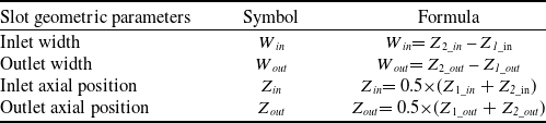
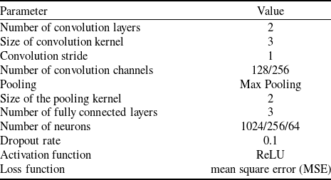

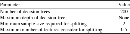

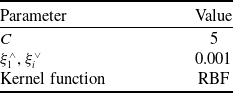
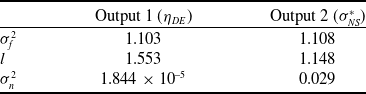
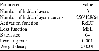


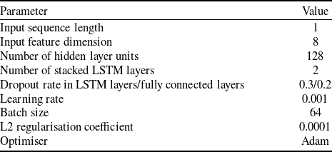



 η
 σNS∗
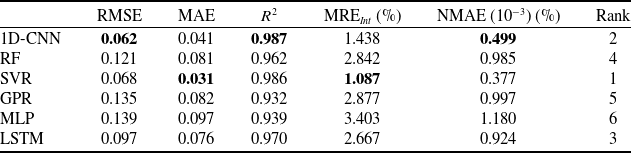
 η
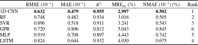
 σNS∗

 η
 σNS∗

 η
 σNS∗

 η
 σNS∗

 η
 σNS∗

 η
 σNS∗

 η
 σNS∗


 η
 σNS∗

 η
 σNS∗

 η
 σNS∗



