


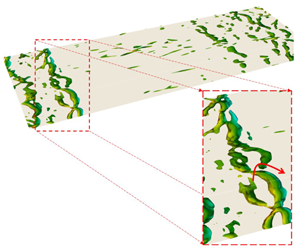


1 Introduction
When an acoustic wave passes over a solid boundary, a thin region is observed near the wall wherein the viscous effect on the wave decays exponentially. This layer is known as the Stokes layer, and its thickness is  $\unicode[STIX]{x1D6FF}_{s}=\sqrt{2\unicode[STIX]{x1D708}/\unicode[STIX]{x1D714}_{f}}$, where
 $\unicode[STIX]{x1D708}$ and
 $\unicode[STIX]{x1D714}_{f}$ are the kinematic viscosity and angular velocity of the wave, respectively. Under favourable conditions, such acoustic waves can lead to steady (acoustic) streaming, i.e. a non-zero steady fluid motion appearing as a result of nonlinear interaction of waves and background flow. This process has been widely investigated in the past few decades thanks to its abundant applications across various disciplines, including microfluidics (Wiklund, Green & Ohlin Reference Wiklund, Green and Ohlin2012), ocean engineering (Scandura Reference Scandura2007) and thermoacoustics (Bailliet et al. Reference Bailliet, Gusev, Raspet and Hiller2001). Extensive reviews on different mechanisms driving the acoustic streaming are given in Riley (Reference Riley2001) and Boluriaan & Morris (Reference Boluriaan and Morris2003). In the present research, we focus on the steady streaming that appears in straight channels due to the external pulsations.
Lord Rayleigh (Reference Rayleigh1884) numerically studied the acoustic streaming formed between two parallel plates, driven by a longitudinal standing wave. He essentially focused on the region outside of the boundary layer and found the outer streaming velocity to be proportional to  $M_{a}^{2}$, where
 $M_{a}=\widetilde{U}/c_{0}$ is the acoustic Mach number,
 $\widetilde{U}$ is the amplitude of velocity oscillations at the source and
 $c_{0}$ represents the speed of sound. Later, Schlichting (Reference Schlichting1932) extended this work to analyse the streaming within an incompressible oscillating boundary layer and suggested that the inner streaming velocity is also
 $O(M_{a}^{2})$. These theoretical approaches were derived only for very small oscillation amplitudes. To assess if the nonlinear effects due to large oscillations are significant, Menguy & Gilbert (Reference Menguy and Gilbert2000) introduced a nonlinear Reynolds number,
 $Re_{nl}=2M_{a}^{2}/Sh^{2}$, where
 $Sh=\unicode[STIX]{x1D6FF}_{s}/(\sqrt{2}\unicode[STIX]{x1D6FF})$ is the shear number and
 $\unicode[STIX]{x1D6FF}$ represents the channel half-width (half the distance between the two parallel plates). The theoretical findings on the streaming velocity mentioned above are valid only if
 $Re_{nl}\ll 1$. Therefore, in practical cases, employing a direct simulation of the Navier–Stokes equations may be necessary. Yano (Reference Yano1999) solved the two-dimensional compressible Navier–Stokes and energy equations to simulate the streaming in a half-wavelength standing-wave resonator. This study showed that, unless at very high frequency or in highly viscous fluids, the amplitude of oscillations initially grows at the rate of
 $O(M_{a}t)$ and reaches a quasi-steady state with periodic shock waves of amplitude
 $O(\sqrt{M_{a}})$. In this case, the streaming velocity is proportional to
 $M_{a}$.
Acoustic streaming has also been used for heat transfer enhancement. Vainshtein, Fichman & Gutfinger (Reference Vainshtein, Fichman and Gutfinger1995) considered a longitudinal standing wave formed between two parallel plates kept at different temperatures and studied the effect of streaming on the heat transfer in this gap. They observed that such a mechanism can enhance the heat transfer up to one order of magnitude compared to the case with only conduction. Aktas, Farouk & Lin (Reference Aktas, Farouk and Lin2005) studied the heat transfer in a shallow enclosure in which the horizontal walls are adiabatic and the sidewalls are kept at different temperatures, where one sidewall oscillates at the resonant and off-design frequencies. Under the resonant conditions, the streaming velocity becomes significant, and the time-averaged heat transfer coefficient ( $\overline{h}$) near the stationary wall increases by almost one order of magnitude. On the contrary, off-design oscillations fail to create a noticeable streaming velocity or a considerable change in
 $\overline{h}$, therefore indicating the significance of resonance in creating time-averaged changes in the flow. Aktas & Ozgumus (Reference Aktas and Ozgumus2010) extended this work to higher
 $Re_{nl}$ and observed shock-wave oscillations (similar to Yano (Reference Yano1999)) in the channel. They also investigated how the formation of the streaming pattern can enhance the heat transport between two fixed horizontal parallel plates.
All the aforementioned studies were carried out for the purely oscillatory cases, while in pulsating flows, the Stokes layer interacts with the background hydrodynamic and thermal boundary layers in a nonlinear fashion. Two dimensionless parameters are conventionally introduced to study such a phenomenon: the ratio of the external wave amplitude to the bulk velocity of the background flow,  $a_{w}=\widetilde{U}/U_{b}$; and the normalized wave frequency,
 ${\unicode[STIX]{x1D714}_{f}}^{+}=\unicode[STIX]{x1D714}_{f}\unicode[STIX]{x1D708}/u_{\unicode[STIX]{x1D70F}}^{2}$, where
 $u_{\unicode[STIX]{x1D70F}}=\sqrt{\unicode[STIX]{x1D70F}_{w}/\unicode[STIX]{x1D70C}}$ is the friction velocity. As long as
 $a_{w}$ is less than 1, the parameter
 ${\unicode[STIX]{x1D714}_{f}}^{+}$ mainly determines the flow regime (Lodahl, Sumer & Fredse Reference Lodahl, Sumer and Fredse1998; Scotti & Piomelli Reference Scotti and Piomelli2001). Generally, low-frequency pulsations (where
 $0.003\lesssim \unicode[STIX]{x1D714}^{+}\lesssim 0.006$) create a thick Stokes layer whose edge may reside in the buffer layer where turbulent mixing is important. As such, a portion of the acoustic energy is extracted from the wave and distributed among the smaller turbulent structures (Weng, Boij & Hanifi Reference Weng, Boij and Hanifi2016). This nonlinear process greatly impacts the oscillatory wave, under specific conditions, and may alter the time-averaged velocity and temperature profiles (Lodahl et al. Reference Lodahl, Sumer and Fredse1998). On the other hand, high-frequency acoustic waves (where
 $0.02\lesssim \unicode[STIX]{x1D714}^{+}\lesssim 0.04$) create a very thin Stokes layer confined within the viscous sublayer. In this region, turbulent mixing is minimal, and the external wave interacts only with the mean background flow. In other words, the period of oscillations is shorter than turbulence time scales; therefore, such waves may not be altered by turbulent processes. A very high-frequency regime (
 $0.04\lesssim \unicode[STIX]{x1D714}^{+}$) has been identified where pulsations can make critical changes in time-averaged turbulent flow properties. Several studies, including Tardu, Binder & Blackwelder (Reference Tardu, Binder and Blackwelder1994) and Scotti & Piomelli (Reference Scotti and Piomelli2001), attributed such behaviour to the pairing of pulsation frequency and bursting frequency of coherent structures in the inner layer suggested by Mizushina, Maruyama & Shiozaki (Reference Mizushina, Maruyama and Shiozaki1974). This observation is supported by the results of Havemann & Narayan Rao (Reference Havemann and Narayan Rao1954), Said et al. (Reference Said, Al-Farayedhi, Habib, Gbadebo, Asghar and Al-Dini1998) and Habib et al. (Reference Habib, Said, Al-Farayedhi, Al-Dini, Asghar and Gbadebo1999).
In the present research, in order to maximize the effect of acoustic pulsation on the flow, we identify the specific conditions required for the external wave to acoustically resonate within the domain. This is achieved using linear stability analysis of the background flow without the excitation. Such information is used to select the frequency and shape of the external acoustic field for making desirable changes in the flow. This resonant frequency is close to the bursting frequency suggested to be able to modify the time-averaged Nusselt number ( $Nu$) and skin friction (
 $C_{f}$) upon pulsation. Moreover, the sensitivity of the flow response to the resonant frequency is assessed by applying external waves of identical amplitude and shape but at off-resonance frequencies. The present research is the first study to achieve ‘acoustic streaming’ in compressible flows, and it opens new avenues towards enhancing the heat transfer without excessive skin-friction losses.
Schematic view of the proposed set-up. The computational domain is of size  $(L_{x},L_{y},L_{z})=(4\unicode[STIX]{x03C0}\unicode[STIX]{x1D6FF},2\unicode[STIX]{x1D6FF},1.5\unicode[STIX]{x03C0}\unicode[STIX]{x1D6FF})$. The shaded area of width
 $L_{f}$ in each unit indicates the region where the effect of acoustic drivers mounted on the sidewalls is modelled via a forcing function of form (2.1).

2 Problem formulation
The proposed test case comprises repeating identical sections of length  $L_{x}$, where each one includes a duct with an array of acoustic drivers mounted on the sidewalls. Figure 1 shows a schematic view of the set-up. By exploiting the geometrical symmetry, we only simulate one unit and impose a periodic boundary condition in the streamwise direction. To avoid complexities associated with the corners and the boundary layer formed on the sidewalls, we focus on the midspan region and implement the periodic boundary condition in the spanwise direction. The effect of acoustic drivers is modelled with an external forcing following a bell-shaped function,
 $$\begin{eqnarray}\boldsymbol{f}_{f}(\mathit{x},t)=A_{f}\exp \left(-\frac{(x-x_{m})^{2}}{L_{f}^{2}}\right)\sin (\unicode[STIX]{x1D714}_{f}t)\,\boldsymbol{e}_{x},\end{eqnarray}$$
where  $A_{f}$ is the forcing amplitude,
 $L_{f}$ represents the length scale of the forcing region with midpoint
 $x_{m}$, and
 $\unicode[STIX]{x1D714}_{f}$ sets the frequency of excitation. This force is added to the momentum equation as the source term, and the work performed by this source on the flow is considered in the energy equation following
 $\boldsymbol{f}_{f}\boldsymbol{\cdot }\boldsymbol{u}$.
3 Numerical methodology
The fully compressible continuity, momentum and energy equations in the Cartesian coordinate system take the non-dimensional forms
 $$\begin{eqnarray}\left.\begin{array}{@{}c@{}}{\displaystyle \frac{\unicode[STIX]{x2202}\unicode[STIX]{x1D70C}}{\unicode[STIX]{x2202}t}}+{\displaystyle \frac{\unicode[STIX]{x2202}}{\unicode[STIX]{x2202}x_{j}}}(\unicode[STIX]{x1D70C}u_{j})=0,\\ {\displaystyle \frac{\unicode[STIX]{x2202}}{\unicode[STIX]{x2202}t}}(\unicode[STIX]{x1D70C}u_{i})+{\displaystyle \frac{\unicode[STIX]{x2202}}{\unicode[STIX]{x2202}x_{j}}}(\unicode[STIX]{x1D70C}u_{i}u_{j})=-{\displaystyle \frac{\unicode[STIX]{x2202}p}{\unicode[STIX]{x2202}x_{i}}}+{\displaystyle \frac{1}{Re}}{\displaystyle \frac{\unicode[STIX]{x2202}}{\unicode[STIX]{x2202}x_{j}}}(\unicode[STIX]{x1D70F}_{ij})+f_{i}\unicode[STIX]{x1D6FF}_{1i},\\ {\displaystyle \frac{\unicode[STIX]{x2202}E}{\unicode[STIX]{x2202}t}}+{\displaystyle \frac{\unicode[STIX]{x2202}}{\unicode[STIX]{x2202}x_{j}}}[(E+p)u_{j}]={\displaystyle \frac{1}{Re}}{\displaystyle \frac{\unicode[STIX]{x2202}}{\unicode[STIX]{x2202}x_{j}}}\left(k{\displaystyle \frac{\unicode[STIX]{x2202}T}{\unicode[STIX]{x2202}x_{j}}}\right)+{\displaystyle \frac{1}{Re}}{\displaystyle \frac{\unicode[STIX]{x2202}}{\unicode[STIX]{x2202}x_{k}}}(\unicode[STIX]{x1D70F}_{jk}u_{j})+f_{i}u_{i}\unicode[STIX]{x1D6FF}_{1i},\end{array}\right\}\end{eqnarray}$$
where  $(x_{1},x_{2},x_{3})=(x,y,z)$ represent streamwise, wall-normal and spanwise directions, and
 $f_{i}\unicode[STIX]{x1D6FF}_{1i}$ indicates a volume forcing in the
 $x$-direction. At each time step, the bulk velocity
 $U_{b}$ is locally computed following
 $$\begin{eqnarray}U_{b}(x,z)={\displaystyle \frac{\displaystyle \int _{0}^{L_{y}}\unicode[STIX]{x1D70C}u\,\text{d}y}{\displaystyle \int _{0}^{L_{y}}\unicode[STIX]{x1D70C}\,\text{d}y}}.\end{eqnarray}$$
Then, the spatially averaged bulk velocity in the entire domain is calculated via
 $$\begin{eqnarray}U_{b,tot}={\displaystyle \frac{\displaystyle \int _{0}^{L_{z}}\!\int _{0}^{L_{x}}U_{b}(x,z)\,\text{d}x\,\text{d}z}{L_{x}L_{z}}}.\end{eqnarray}$$
If  $U_{b,tot}$ is different from the target value,
 $U_{b,target}$, a uniform forcing term is added to the entire domain, in order to retain the target value that corresponds to a constant mass flow rate. This is a common practice when simulating turbulent channel flow, which is followed by Coleman, Kim & Moser (Reference Coleman, Kim and Moser1995) for compressible case, and by Lévêque et al. (Reference Lévêque, Toschi, Shao and Bertoglio2007) in the incompressible case. Such a forcing strategy allows the pressure gradient to take any non-uniform distribution within the domain (for example, in the pulsating case), given that the overall mass flow rate is constant. For non-dimensionalization purposes, the reference temperature, velocity and length scales are, respectively, the wall temperature (
 $T_{w}$), speed of sound at the wall temperature (
 $c_{w}$) and channel half-width (
 $\unicode[STIX]{x1D6FF}$). Therefore, the amplitude of forcing in (2.1) is non-dimensionalized by
 $\overline{\unicode[STIX]{x1D70C}}c_{w}^{2}/\unicode[STIX]{x1D6FF}$. The total energy (
 $E$) and viscous stress tensor (
 $\unicode[STIX]{x1D70F}^{ij}$) read
 $$\begin{eqnarray}E={\displaystyle \frac{p}{\unicode[STIX]{x1D6FE}-1}}+{\displaystyle \frac{1}{2}}\unicode[STIX]{x1D70C}u_{i}u_{i},\quad \unicode[STIX]{x1D70F}_{ij}=\unicode[STIX]{x1D707}\left({\displaystyle \frac{\unicode[STIX]{x2202}u_{i}}{\unicode[STIX]{x2202}x_{j}}}+{\displaystyle \frac{\unicode[STIX]{x2202}u_{j}}{\unicode[STIX]{x2202}x_{i}}}-{\displaystyle \frac{2}{3}}{\displaystyle \frac{\unicode[STIX]{x2202}u_{k}}{\unicode[STIX]{x2202}x_{k}}}\unicode[STIX]{x1D6FF}_{ij}\right),\end{eqnarray}$$
where the molecular dynamic viscosity follows the exponential form  $\unicode[STIX]{x1D707}/\unicode[STIX]{x1D707}_{w}=(T/T_{w})^{0.7}$. This set of equations along with the equation of state for the perfect gas
 $p=(1/\unicode[STIX]{x1D6FE})\unicode[STIX]{x1D70C}T$ are discretized in space using a sixth-order staggered finite difference method (Nagarajan, Lele & Ferziger Reference Nagarajan, Lele and Ferziger2003). A third-order Runge–Kutta method is employed for time advancement.
Linear stability analysis (LSA) is a widely popular tool to identify and control low-frequency unsteadiness in laminar flows (Schmid & Henningson Reference Schmid and Henningson2000). On the other side, turbulent flows experience broadband fluctuations in all quantities, accompanied by low-frequency structures responsible for significant coherent changes in the domain. Several authors have studied LSA of the time-averaged flow quantities in a turbulent channel flow in order to analyse the turbulent coherent structures, including Reynolds & Tiederman (Reference Reynolds and Tiederman1967), Reynolds & Hussain (Reference Reynolds and Hussain1972) and Jimenez et al. (Reference Jimenez, Uhlmann, Pinelli and Kawahara2001). The present research follows the same approach to analyse the unexcited (background) turbulent channel flow and identify the optimal excitation frequency.
Linearized Navier–Stokes equations are derived by first-order expansion of flow variables about the equilibrium state, i.e.  $q(\boldsymbol{x},t)=\overline{q}(\boldsymbol{x})+\unicode[STIX]{x1D700}q^{\prime }(\boldsymbol{x},t)+\mathit{O}(\unicode[STIX]{x1D700}^{2})$. Substituting this form in the compressible Navier–Stokes equations (3.1) gives
 $$\begin{eqnarray}\displaystyle {\displaystyle \frac{\text{d}q^{\prime }}{\text{d}t}}={\mathcal{L}}q^{\prime }, & & \displaystyle\end{eqnarray}$$
where  ${\mathcal{L}}$ is an operator of time-averaged quantities and spatial derivatives, and therefore independent of time (Malik Reference Malik1990). Here, we have used the spectral Chebyshev method to discretize these spatial derivatives (Trefethen Reference Trefethen2000). The solution of this ordinary differential equation may take the form
 $q^{\prime }(\boldsymbol{x},t)=\hat{q}(\boldsymbol{x})$
 $\exp (-\text{j}\unicode[STIX]{x1D714}t)$ allowing the modal analysis of the perturbation dynamics. Applying this form to (3.3) results in an eigenvalue problem,
 $$\begin{eqnarray}\displaystyle {\mathcal{A}}\hat{q}=\unicode[STIX]{x1D714}\hat{q}, & & \displaystyle\end{eqnarray}$$
where  $\unicode[STIX]{x1D714}$ is the complex angular velocity. In the present work, the base flow as well as boundary conditions are homogeneous in the streamwise and spanwise directions, and therefore the perturbation form is simplified to
 $q^{\prime }(\boldsymbol{x},t)=\hat{q}(y)\text{e}^{\text{j}(kx+\unicode[STIX]{x1D6FD}z)}\text{e}^{-\text{j}\unicode[STIX]{x1D714}t}$, where
 $k$ and
 $\unicode[STIX]{x1D6FD}$ are spatial wavenumbers in the streamwise and spanwise directions, respectively.
We consider the time-averaged quantities of the unexcited case as the equilibrium state solution,  $\overline{q}(\boldsymbol{x})$. The validity of this choice can be justified by analysing the time scale of different terms involved in the equation for the evolution of turbulent fluctuations. As explained by Lee, Kim & Moin (Reference Lee, Kim and Moin1990) and Jiménez (Reference Jiménez2013), in the regions where the time scale of nonlinear terms is much larger than that of the linear terms, the effect of nonlinear components would be minimal, and therefore the linearized Navier–Stokes equations can represent the dynamics of fluctuations. The time scale of the linear terms is
 $O(1/S)$, where
 $S$ is the mean shear, and the time scale of the nonlinear terms is suggested to be
 $O(l_{\unicode[STIX]{x1D700}}/(\overline{u_{i}^{\prime }u_{i}^{\prime }})^{1/2})$, where
 $l_{\unicode[STIX]{x1D700}}=(\overline{u_{i}^{\prime }u_{i}^{\prime }})^{3/2}/\unicode[STIX]{x1D700}$ is the dissipation length scale and
 $\unicode[STIX]{x1D700}=\unicode[STIX]{x1D708}\overline{\unicode[STIX]{x2202}u_{i}^{\prime }/\unicode[STIX]{x2202}x_{j}\unicode[STIX]{x2202}u_{i}^{\prime }/\unicode[STIX]{x2202}x_{j}}$ is the dissipation rate of turbulent kinetic energy. The ratio of these two time scales is known as the shear parameter,
 $S^{\ast }=(S\overline{u_{i}^{\prime }u_{i}^{\prime }})/\unicode[STIX]{x1D700}$, which should be large enough to assume the linearization to hold. This condition is met near the wall (
 $S^{\ast }$ remains around 10 up to
 $y/\unicode[STIX]{x1D6FF}\lesssim 0.6$), whereas on approaching the channel core where the magnitude of shear decreases, this assumption may not be valid (Jiménez Reference Jiménez2013). It should also be noted that we only include the molecular viscosity (
 $\overline{\unicode[STIX]{x1D707}}$) in the
 ${\mathcal{L}}$ operator of (3.3).
In the present study, we apply the forcing (2.1) to the bulk of the flow in the streamwise direction, i.e. only  $f_{x}\neq 0$. Studying the cases where
 $\unicode[STIX]{x1D6FD}\neq 0$ requires a source (of
 $f_{x}$) with variable strength in the spanwise direction. Creating such forcing near the wall is a common practice (via Lorentz forces or by roughness elements); however, this is not the case where we need to apply such forcing to the bulk of the flow, which is the objective of the present paper. Therefore, we have decided to analyse only the cases with
 $\unicode[STIX]{x1D6FD}=0$.
Time-averaged (a) streamwise velocity, and (b) temperature and density, and (c) root-mean-square fluctuating velocity components at  $Re_{b}=3000$ and two different bulk Mach numbers along the channel height. Results of the present simulations at
 $M_{b}=1.5$ (——), Coleman et al. (Reference Coleman, Kim and Moser1995) at
 $M_{b}=1.5$ (○), and present study at
 $M_{b}=0.75$ (– – – –).

4 Results and discussion
This section first focuses on the simulation of the flow field without external excitation. These results are compared with the literature to assess the accuracy of our computational tool. Time-averaged flow quantities serve as the base flow for the linearized Navier–Stokes analysis. Thereafter, we investigate the effect of acoustic excitation in the same flow configurations and analyse the modified boundary layer characteristics.
4.1 Unexcited flow simulation
The computational set-up consists of two parallel isothermal plates of size  $L_{x}\times L_{z}=4\unicode[STIX]{x03C0}\unicode[STIX]{x1D6FF}\times 1.5\unicode[STIX]{x03C0}\unicode[STIX]{x1D6FF}$ separated by a distance
 $L_{y}=2\unicode[STIX]{x1D6FF}$. The Reynolds number based on bulk velocity is
 $Re_{b}=\overline{\unicode[STIX]{x1D70C}}U_{b}\unicode[STIX]{x1D6FF}/\unicode[STIX]{x1D707}_{w}=3000$ and, to analyse the effect of flow compressibility on the results, two Mach numbers corresponding to the subsonic (
 $M_{b}=U_{b}/c_{w}=0.75$) and supersonic (
 $M_{b}=1.5$) regimes are considered. The computational domain is discretized using
 $N_{x}\times N_{y}\times N_{z}=144\times 128\times 96$ cells, resulting in
 $(\unicode[STIX]{x0394}x^{+},\unicode[STIX]{x0394}y_{min}^{+},\unicode[STIX]{x0394}z^{+})\approx (19,0.24,10.7)$ for the supersonic and
 $(\unicode[STIX]{x0394}x^{+},\unicode[STIX]{x0394}y_{min}^{+},\unicode[STIX]{x0394}z^{+})\approx (17,0.21,9.7)$ for the subsonic cases. Calculations on a finer grid, with 1.5 times more points in each direction, show little to no variations in temporal statistics. Time-averaged streamwise velocity, density and temperature profiles as well as the root-mean-square (r.m.s.) values of fluctuating velocity components are illustrated in figure 2. The supersonic case is identical to the set-up studied by Coleman et al. (Reference Coleman, Kim and Moser1995). Comparing the results of the present simulation with the reference values (Coleman et al. Reference Coleman, Kim and Moser1995) in figure 2 shows a good agreement in terms of the first- and second-order statistics. One significant effect of compressibility is observed in the temperature profiles, where the viscous heating increases the centreline temperature following
 $T_{c}-T_{w}\propto {M_{b}}^{2}$. As such, the core region of the flow is approximately 8.7 % and 37 % hotter than the walls in the subsonic and supersonic cases, respectively. This is expected to provide a proper contrast when analysing the effect of acoustic excitation on the heat transfer characteristics.
Eigenvalue spectra of compressible channel flow at  $Re_{b}=3000$ (a,e) along with the shear stress
 $\widehat{uv}$ and heat flux
 $\widehat{Tv}$ associated with modes
 $R_{1}$ (d,h),
 $W_{1}$ (c,g) and
 $L_{1}$ (b,f). Panels (a–d) correspond to the supersonic case
 $M_{b}=1.5$ and (e–h) represent the subsonic case
 $M_{b}=0.75$. Streamwise wavenumber is
 $k=0.5$. Labels
 $R_{1}$ and
 $L_{1}$ denote the fast and slow acoustic modes, respectively, while
 $W_{1}$ and
 $W_{2}$ are wall modes.

4.2 Linearized Navier–Stokes analysis
We solve the linearized Navier–Stokes equations (3.3) in order to investigate different families of modes present in this flow configuration and identify the ones that are expected to create an effective increase in wall heat transfer throughout the channel. The streamwise wavenumber is considered to be  $k=0.5$ corresponding to the largest wave fitting in the domain of length
 $L_{x}=4\unicode[STIX]{x03C0}$.
The eigenvalue spectra in both subsonic and supersonic cases are shown in figure 3(a,e). This figure focuses on the most unstable modes in the spectrum. The operators  $\text{Re}\{\cdot \}$ and
 $\text{Im}\{\cdot \}$ return the real and imaginary parts of a variable. The horizontal axis represents the propagation speed of each mode and the vertical axis shows the associated growth rate. The dashed line specifies the threshold of neutrally stable modes, so that modes closer to this line experience slower decay rate. All modes are stable, in the absence of external forcing. Similar results are also reported by Friedrich & Bertolotti (Reference Friedrich and Bertolotti1996) using the parabolized stability equations. These findings are consistent with those of Reynolds & Hussain (Reference Reynolds and Hussain1972), who observed that LSA of mean profiles corresponding to an incompressible turbulent channel flow remains stable up to
 $Re_{\unicode[STIX]{x1D70F}}=\mathit{O}(1000)$. As studied by Jimenez et al. (Reference Jimenez, Uhlmann, Pinelli and Kawahara2001) and Del Alamo & Jimenez (Reference Del Alamo and Jimenez2006), we can link the stable modes with the largest temporal growth rates to the near-wall coherent structures. Here, we use the information provided by the LSA to decide which mode should be excited to create the target changes in the flow.
In the present configuration, four major families of modes are observed: the ‘bulk’ modes that form a hook shape and travel downstream with the bulk velocity of the flow, the ‘fast acoustic’ modes (e.g.  $R_{1}$) that are positioned on the right and the ‘slow’ modes (e.g.
 $L_{1}$) appearing on the left side of the bulk modes, along with the other two isolated modes shown in figure 3 representing the wall modes
 $W_{1,2}$. To further analyse these modes’ properties, two parameters are defined based on their corresponding eigenfunctions:
 $$\begin{eqnarray}\left.\begin{array}{@{}c@{}}\widehat{uv}={\displaystyle \frac{2}{{\mathcal{T}}}}\displaystyle \int _{0}^{{\mathcal{T}}}\text{Re}\{u^{\prime }\}\text{Re}\{v^{\prime }\}\,\text{d}t=\text{Re}\{\hat{u} \,\hat{v}^{\ast }\}\quad \mathit{mode~shear~stress},\\ \widehat{Tv}={\displaystyle \frac{2}{{\mathcal{T}}}}\displaystyle \int _{0}^{{\mathcal{T}}}\text{Re}\{T^{\prime }\}\text{Re}\{v^{\prime }\}\,\text{d}t=\text{Re}\{\widehat{T}\,\hat{v}^{\ast }\}\quad \mathit{mode~heat~flux},\end{array}\right\}\end{eqnarray}$$
where  ${\mathcal{T}}$ represents the period,
 $\hat{u}$,
 $\hat{v}$ and
 $\widehat{T}$ are streamwise velocity, wall-normal velocity and temperature eigenfunctions and superscript
 $\ast$ denotes complex conjugate. Figure 3 illustrates these quantities for three modes
 $R_{1}$,
 $W_{1}$ and
 $L_{1}$ at two different Mach numbers. Modes belonging to the same family exhibit similar behaviour; however, near-wall changes are more pronounced in the supersonic case due to larger mean flow gradients in this condition.
Wall modes  $W_{i}$ have a large decay rate and, in the case of excitation, can only affect the near-source region. Moreover, their corresponding added shear stress is significantly higher than the added heat flux, and therefore they cannot be the ideal mode for making an effective heat transfer enhancement. Applying an external forcing activated only near the wall or modifying the wall boundary condition, for instance by employing a Darcy-type porous medium (Tilton & Cortelezzi Reference Tilton and Cortelezzi2008; Rahbari & Scalo Reference Rahbari and Scalo2017a) or acoustic liners (Rahbari & Scalo Reference Rahbari and Scalo2017b), often results in the excitation of this mode.
Slow acoustic (or left-running) modes  $L_{1}$ experience a faster decay rate than the
 $R_{1}$ modes, limiting their ability to make a global change in the flow. This mode’s corresponding heat flux is still less than the associated shear stress while also showing a
 $180^{\circ }$ phase difference.
Mode  $R_{1}$, on the other hand, has the largest imaginary part, which translates into the lowest decay rate and therefore, if excited, can make a lasting change in the flow. Moreover, the heat flux corresponding to this mode is comparable with its shear stress near the boundaries. Therefore, the
 $R_{1}$ mode is chosen as the ‘resonant mode’ for the acoustic excitation.
Estimation of mode  $R_{1}$’s velocity in the present test case may not be straightforward since the temperature rises up to 37 % (in case C1:
 $M_{b}=1.5$) and 8.7 % (in case C2:
 $M_{b}=0.75$) from the wall to the centreline, and therefore the speed of sound changes considerably across the channel. In case C1,
 $\bar{U}_{centreline}+\bar{c}_{centreline}=2.91$, while the LSA gives
 $c_{R_{1}}=2.73$. In case C2,
 $\bar{U}_{centreline}+\bar{c}_{centreline}=1.91$, whereas the LSA shows
 $c_{R_{1}}=1.81$.
The optimal wall-normal distribution of forcing term ( $A_{f}$ in (2.1)) can be determined following the method of Lagrangian multipliers developed by Browne et al. (Reference Browne, Rubio, Ferrer and Valero2014) in the discrete framework. However, in the present study,
 $A_{f}$ is assumed to be uniform along the channel height for simplicity and ease of future experimental implementation.
4.3 Fully nonlinear Navier–Stokes simulations
After selecting the excitation frequency, fully nonlinear Navier–Stokes equations are solved considering the forcing function of form (2.1). Given the equation (3.1), the periodic forcing acts as a pulsating pressure gradient with a Gaussian distribution function applied only in the forcing region, in which the maximum-to-minimum amplitude equals  $2A_{f}$. In addition to studying the acoustic excitation at the resonant frequency at each Mach number, two more cases (labelled as C3 and C4) are also investigated in order to analyse the effect of off-design excitation on the flow. Moreover, we study three cases, namely A1 to A3, identical to C2 but at different forcing amplitudes, to reveal the impact of
 $A_{f}$ on the perturbation dynamics and time-averaged flow quantities. Simulations D1 and D2 explore the resonance phenomenon at lower frequencies by considering larger domain lengths, i.e.
 $L_{x}=6\unicode[STIX]{x03C0}$ and
 $8\unicode[STIX]{x03C0}$ (corresponding to
 $k=2/3$ and
 $k=1/4$). Extension of the results obtained in case C2 to a higher Reynolds number, namely at
 $Re_{b}=6000$, is investigated in case I1. The simulation parameters for all the aforementioned cases are summarized in table1.
The non-dimensional Stokes layer thickness in all cases is very close to the buffer layer threshold of  $y^{+}\approx 5$. The selected range for the excitation frequencies includes the lowest ‘resonant’ frequency that fits in the studied computational domain. In C1 to C4 and A1 to A3, a computational domain identical to the unexcited case (§ 4.1) is adopted. To assess the sensitivity of findings to the computational grid, case C1 is repeated with grid size
 $N_{x}\times N_{y}\times N_{z}=216\times 192\times 144$ (1.5 times grid points in each direction compared to the initial set-up), and little to no variation is observed in temporal statistics. Similarly, the effect of domain size on the results is studied by simulating a channel of length
 $2L_{x}$ with two identical acoustic drivers separated by distance
 $L_{x}$. This case also reproduced temporal statistics that closely follow those of case C1, therefore indicating that the box size is sufficiently long in this analysis.
Simulation parameters for the acoustically excited cases. The length of the forcing region in all cases is set to  $L_{f}=0.447\unicode[STIX]{x1D6FF}$.

In order to analyse the system response to the external fluctuations, we need to clearly differentiate the externally induced perturbations from the background turbulent field. To this aim, we perform two separate sets of simulations for each case, one with the forcing (referred to as the ‘excited’ case) and the other without any external fluctuations (‘unexcited’ case). Both simulations are initialized with identical flow fields, and all other simulation parameters, including the grid and time step size, are kept unchanged. The perturbation field ( $\unicode[STIX]{x1D6FF}q$) reads
 $$\begin{eqnarray}\unicode[STIX]{x1D6FF}q(\boldsymbol{x},t)=q_{\mathit{exc}}(\boldsymbol{x},t)-q_{\mathit{unexc}}(\boldsymbol{x},t),\end{eqnarray}$$
where  $q_{\mathit{exc}}$ represents a generic flow quantity in the excited configuration and
 $q_{\mathit{unexc}}$ corresponds to the same quantity in the unexcited case.
Figure 4 shows the temporal evolution of the temperature perturbations at the channel centre spatially averaged within the forcing region. In the supersonic case, C1 (figure 4a), the external forcing is translated into temperature perturbations of amplitude 2 % of  $T_{w}$ in the first cycle. Thereafter, this amplitude grows in three different stages. Initially, we observe an exponential growth. Dashed lines show this trend and the detailed view of region (i) suggests the pure sinusoidal form of the perturbations representing a linear (modal) process. In the second stage, the growth rate decreases followed by a steepening in the acceleration phase of the forcing period, which indicates a weakly nonlinear process. Distortions in the pure sinusoidal form of the perturbations manifest higher-frequency waves that appear as a result of nonlinear interactions. Finally, after 10 cycles, the perturbation amplitude remains nearly constant, which marks the limit-cycle region. In this section, immediately after starting each period, the temperature perturbation rises significantly and dissipates gradually. This implies the broadband response of the system to a single-frequency force, which, in turn, demonstrates the highly nonlinear nature of this region (see region (ii)). Similar behaviour is observed in subsonic configuration, C2 (figure 4b). Although the amplitude of
 $\unicode[STIX]{x1D6FF}T$ in this case is always smaller than that of the supersonic configuration, the limit cycle is achieved in fewer periods, suggesting that the nonlinear process starts earlier.
History of temperature perturbation  $\unicode[STIX]{x1D6FF}T=T_{\mathit{exc}}-T_{\mathit{unexc}}$ at the centre of the forcing region at
 $Re_{b}=3000$ and two Mach numbers: (a) case C1,
 $M_{b}=1.5$, and (b) case C2,
 $M_{b}=0.75$. The results are downsampled to eight instants per period.

The next step is to analyse the effect of acoustic excitation on the heat and momentum transfer near the wall. Two parameters, shear enhancement factor (SEF) and thermal enhancement factor (TEF), are defined based on the space-averaged skin-friction coefficient ( $C_{f}$) and Nusselt number (
 $Nu$) to quantitatively study this process:
 $$\begin{eqnarray}\text{SEF}={\displaystyle \frac{C_{f,\mathit{exc}}}{C_{f,\mathit{unexc}}}}\quad \text{and}\quad \text{TEF}={\displaystyle \frac{Nu_{\mathit{exc}}}{Nu_{\mathit{unexc}}}},\end{eqnarray}$$
where
 $$\begin{eqnarray}\displaystyle C_{f}={\displaystyle \frac{\left.\unicode[STIX]{x1D707}_{w}{\displaystyle \frac{\unicode[STIX]{x2202}U}{\unicode[STIX]{x2202}y}}\right|_{w}}{0.5\unicode[STIX]{x1D70C}U_{b}^{2}}}\quad \text{and}\quad Nu={\displaystyle \frac{\left.{\displaystyle \frac{\unicode[STIX]{x2202}}{\unicode[STIX]{x2202}y}}(T-T_{w})\right|_{w}}{(T_{b}-T_{w})/\unicode[STIX]{x1D6FF}}}, & & \displaystyle \nonumber\end{eqnarray}$$
and the bulk temperature ( $T_{b}$) is calculated following the same procedure as described for computing the total bulk velocity
 $U_{b,tot}$. This quantity is calculated at each time step for all cases separately. Considering the modified Reynolds analogy (Chilton–Colburn equation),
 $$\begin{eqnarray}\displaystyle C_{f}={\displaystyle \frac{Nu}{Re_{b}\,Pr^{1/3}}}, & & \displaystyle \nonumber\end{eqnarray}$$
one may find the Nusselt number as a linear function of the skin friction (or vice versa). In the unexcited condition, this relationship holds at  $Re_{b}=3000$ and
 $M_{b}=1.5$ with less than 1 % error, and at the same Reynolds number and
 $M_{b}=0.75$, with less than 3 % error. If we assume this analogy to be valid in the excited flow configuration as well,
 $$\begin{eqnarray}\displaystyle C_{f,\mathit{exc}}={\displaystyle \frac{Nu_{\mathit{exc}}}{Re_{b}\,Pr^{1/3}}}. & & \displaystyle \nonumber\end{eqnarray}$$
Hence,  $C_{f,\mathit{exc}}/C_{f,\mathit{unexc}}=Nu_{\mathit{exc}}/Nu_{\mathit{unexc}}$. Given the definitions of shear and thermal enhancement factors (4.3), this implies
 $\text{SEF}=\text{TEF}$. Therefore, we expect SEF and TEF to closely follow each other, and comparing these two quantities is appropriate. In regions where an offset is observed between these two quantities, one may conclude that the Reynolds analogy (or any simple linear relationship between
 $C_{f}$ and
 $Nu$) does not hold.
History of the space-averaged SEF and TEF at  $Re_{b}=3000$ and two Mach numbers: (a) C1,
 $M_{b}=1.5$, and (b) C2,
 $M_{b}=0.75$. The results are downsampled to eight instants per period. EF, enhancement factor.

At different Mach numbers, we have different heat loads  $(T_{b}-T_{w})\propto M_{b}^{2}$; essentially, the heat load at
 $M_{b}=0.75$ is four times smaller than that at
 $M_{b}=1.5$. Since the amplitudes of the excitation (
 $\unicode[STIX]{x1D6FF}T$) in both cases are similar, we expect the heat transfer process at the smaller
 $M_{b}$ to experience stronger alteration due to the excitation. Figure 5 presents the history of SEF and TEF over 50 periods for both C1 and C2 cases. These two quantities share similar trends; they both start from unity (by definition), grow rapidly in time and finally oscillate around some mean value. Acoustic excitation leads to higher thermal enhancement compared to the skin-friction augmentation. The difference between SEF and TEF is significantly more pronounced in the subsonic configuration (C2), although having smaller
 $\unicode[STIX]{x1D6FF}T$ amplitude. Averaging these quantities over 100 excitation periods shows
 $\overline{\text{TEF}}=1.101$ and
 $\overline{\text{SEF}}=1.084$ for the supersonic case (C1) and
 $\overline{\text{TEF}}=1.109$ and
 $\overline{\text{SEF}}=1.053$ for the subsonic case (C2). Therefore, heat transfer enhancement due to the excitation is 20 % higher than the skin-friction augmentation in C1, while in C2 configuration, acoustic excitation enhanced the heat transfer almost twice as much as the skin friction.
The adiabatic wall temperature  $T_{aw}$ is defined as the temperature that a wall would acquire if it were thermally insulated. Here, we estimate this quantity via
 $T_{aw}=T_{c}[1+Pr^{1/3}((\unicode[STIX]{x1D6FE}-1)/2)M_{c}^{2}]$, where
 $T_{c}$ and
 $M_{c}$ are static temperature and local Mach number at the channel centre (White & Corfield Reference White and Corfield2006). This quantity for the supersonic case is approximately
 $T_{aw}=1.91$, and for the subsonic case is
 ${\approx}1.22$, while the wall temperature in both cases is constant at
 $T_{w}=1$. Upon finding
 $T_{aw}$, one may calculate the heat transfer coefficient as
 $h=q^{\prime \prime }/T_{aw}-T_{w}$. According to Maffulli & He (Reference Maffulli and He2014),
 $q^{\prime \prime }$ is not a linear function of
 $T_{aw}-T_{w}$; instead, the slope
 $\unicode[STIX]{x2202}q^{\prime \prime }/\unicode[STIX]{x2202}(T_{aw}-T_{w})$ decreases as
 $(T_{aw}-T_{w})$ becomes smaller. Therefore, in response to a constant change in wall temperature (
 $\unicode[STIX]{x1D6FF}T_{w}$), one may observe a larger change of heat flux in the supersonic case. On the other hand, in the case of a constant change in heat flux (
 $\unicode[STIX]{x1D6FF}q^{\prime \prime }$), for example due to the excitation, the variation of this slope, i.e.
 $h$, may be more pronounced in the subsonic condition. Hence, we expect that the acoustic pulsation with similar amplitude would be more effective in modifying the TEF of the subsonic case compared to the supersonic counterpart.
Instantaneous temperature perturbation field ( $\unicode[STIX]{x1D6FF}T$) for acoustically excited supersonic turbulent boundary layer. A top view at the bottom wall
 $y^{+}\approx 4$ for four instants of one period. Panels (a–d) and (e–h) respectively correspond to one cycle within regions (i) and (ii) in figure 4.

We investigate the effect of acoustic excitation on the near-wall turbulent structures by analysing the temperature perturbation field. Since both C1 and C2 show a similar behaviour, discussion in this section is limited to the supersonic set-up (C1). Figure 6 illustrates the instantaneous temperature perturbations near the bottom wall (at  $y^{+}\approx 4$) for two separate forcing cycles. Figure 6(a–d) correspond to an earlier stage of the excitation process, i.e. region (i) of figure 4, and show the variation of
 $\unicode[STIX]{x1D6FF}T$ at four different instants of one period. The prescribed forcing is translated into the passage of a travelling wave with an amplitude of
 ${\approx}5.5\,\%\,T_{w}$. Weakly nonlinear interaction of the acoustic wave and near-wall streamwise streaks is noticeable in the form of fluctuations superimposed on the spatial sinusoidal pattern and excessively hot or cold spots. Figure 6(e–h) show the passage of an acoustic wave in the limit-cycle region. The wave front creates a strong spanwise structure travelling downstream with speed
 $c_{x}=4\unicode[STIX]{x03C0}/{\mathcal{T}}=2.73$ (non-dimensionalized by
 $c_{w}$) followed by a wake of weaker rollers. In this case, the amplitude of perturbations increases up to
 $22\,\%\,T_{w}$, with several locations experiencing unusually high and low temperatures. Classic near-wall turbulent structures are more evident in these panels by streamwise low-speed streaks disrupting the wave front and significantly modulating the region behind it.
Time– $x$ representation of the spanwise-averaged temperature field near the bottom wall at
 $y^{+}\approx 4$ (a) and at the channel centre (b), over one pulsation cycle in the limit-cycle region.

Contours of streaming velocity  $U_{st}$ (a) and temperature
 $T_{st}$ (b) for an acoustically excited supersonic channel flow at
 $Re_{b}=3000$ and
 $M_{b}=1.5$ with
 $A_{f}=0.5$ and
 $\unicode[STIX]{x1D714}_{f}=2\unicode[STIX]{x03C0}/4.59$ over
 $t/{\mathcal{T}}\in [10,90]$. Time averaging is taken for eight snapshots per period, therefore deliberately neglecting the contribution of wavenumbers greater than four.

Figure 7 displays the time–space temperature field averaged in the spanwise direction once the perturbations are saturated, i.e. in region (ii) in figure 4(a). This representation allows one to identify the different speeds at which perturbations evolve. Near the bottom wall at  $y^{+}\approx 4$ (figure 7a), the wave front is visible along with the rollers that appear in the wake region, retaining a constant speed across the domain. At the channel centre (figure 7b), after the passage of the wave front, one can observe relatively strong waves that propagate downstream at very slow rates (high slopes in the
 $t{-}x$ plane), and therefore, over one pulsation period
 ${\mathcal{T}}$, are confined within a narrow region in
 $x$. This suggests the formation of structures with time scale
 $\ll {\mathcal{T}}$ and length scale
 $\ll L_{x}$, which can drive the streaming process.
Streaming velocity and temperature, defined as  $U_{st}=\overline{U}_{\mathit{exc}}-\overline{U}_{\mathit{unexc}}$ and
 $T_{st}=\overline{T}_{\mathit{exc}}-\overline{T}_{\mathit{ubnexc}}$, for case C1 are illustrated in figure 8. Time averaging is performed within
 $t/{\mathcal{T}}\in [10,90]$ so as to include only the limit-cycle oscillations. Moreover, only eight snapshots per period are used for time averaging, which consequently neglects the contribution of wavenumbers greater than four in the results. This procedure is adopted to give a generic view of streaming flow features. As a result of the nonlinear interaction between the perturbations and the background flow, as well as among perturbations themselves, a periodic pattern appears in both
 $T_{st}$ and
 $U_{st}$. The regions with positive streaming values appear to take larger magnitudes and stay closer to the wall; therefore, one may qualitatively infer that the SEF and TEF (spatially averaged along the channel length) would be greater than unity. Larger TEF compared to SEF for this flow condition may also be attributed to the locations of positive
 $T_{st}$, which reside at shorter distances from the wall compared to those of
 $U_{st}$.
Phase-locked averaged temperature contours (at  $t/{\mathcal{T}}=1/4$) for (a) supersonic (C1) and (e) subsonic cases (C2). Maximum and minimum values are truncated for better visualization. (b,f) Spatial DFT of this field. (c,g) The amplitude of the dominant mode (
 $k=0.5$) along with the temperature eigenfunction of the most unstable mode identified by LSA. (d,h) The same procedure repeated for the streamwise velocity.

4.4 On the efficacy of linear stability analysis in selecting the optimal modes
An instantaneous quantity  $\unicode[STIX]{x1D719}(\boldsymbol{x},t)$ can be decomposed into ‘steady’, ‘harmonic’ and ‘random’ components, i.e.
 $\unicode[STIX]{x1D719}(\boldsymbol{x},t)=\overline{\unicode[STIX]{x1D719}(\boldsymbol{x})}+\widetilde{\unicode[STIX]{x1D719}(\boldsymbol{x},t)}+\unicode[STIX]{x1D719}^{\prime }(\boldsymbol{x},t)$. The harmonic term is
 $$\begin{eqnarray}\widetilde{\unicode[STIX]{x1D719}(\boldsymbol{x},t)}=\langle \unicode[STIX]{x1D719}(\boldsymbol{x},t)\rangle -\overline{\unicode[STIX]{x1D719}(\boldsymbol{x})}\quad \text{where }\langle \unicode[STIX]{x1D719}(\boldsymbol{x},t)\rangle ={\displaystyle \frac{1}{N}}\mathop{\sum }_{n=0}^{N}\unicode[STIX]{x1D719}(\boldsymbol{x},t+n{\mathcal{T}}).\end{eqnarray}$$
The term  $\langle \unicode[STIX]{x1D719}(\boldsymbol{x},t)\rangle$ represents the phase-locked averaging and
 ${\mathcal{T}}=2\unicode[STIX]{x03C0}/\unicode[STIX]{x1D714}_{f}$ is the period of excitation. Figures 9(a) and 9(e) illustrate the harmonic component of temperature,
 $\widetilde{T}$, at phase
 $t/{\mathcal{T}}=1/4$ in both supersonic (C1) and subsonic (C2) cases. These components are calculated by averaging in the spanwise direction as well as temporally within
 $t/{\mathcal{T}}\in [0,50]$. The results share fundamental similarities, e.g. a significant change in the bulk of the flow accompanied by near-wall spanwise structures whose sizes strongly depend on
 $M_{b}$. If no nonlinear interactions were involved, either among the superimposed waves or between the waves and the background turbulent field, we would expect to observe a single-frequency harmonic field; however, the present results suggest the presence of higher-frequency changes. A spatial discrete Fourier transform (DFT) is employed to extract the components corresponding to different wavenumbers. The highest amplitude is associated with
 $k=0.5$, the wavenumber we set in the LSA. Higher-frequency components possess several times smaller amplitudes and are created as a result of nonlinear interactions in the flow. We also compare the amplitude of
 $\widetilde{T}$ and
 $\widetilde{U}$ (harmonic component of streamwise velocity) corresponding to
 $k=0.5$ against the mode shapes predicted by the LSA (performed on time-averaged unexcited flow quantities) in figure 9(c,d) for C1 and figure 9(g,h) for C2. The results show an excellent agreement between these two profiles, suggesting that the proposed technique resulted in exciting the specific mode identified by LSA.
(a) History of SEF and TEF as well as (b) temperature perturbation  $\unicode[STIX]{x1D6FF}T$ at the centre of the forcing region at
 $M_{b}=1.5$ subjected to off-design excitation frequencies. Case C3 in table 1 with
 $\unicode[STIX]{x1D714}_{f}=2\unicode[STIX]{x03C0}/4.00$ is represented by black and case C4 with
 $\unicode[STIX]{x1D714}_{f}=2\unicode[STIX]{x03C0}/5.00$ is shown as grey. On the left SEF (— ⋅ ⋅ —) and TEF (——) overlap throughout the process. The results are downsampled to eight instants per period.

We consider two additional cases, C3 and C4, excited at off-optimal frequencies, namely  $\unicode[STIX]{x1D714}_{3}=2\unicode[STIX]{x03C0}/4.00$ and
 $\unicode[STIX]{x1D714}_{4}=2\unicode[STIX]{x03C0}/5.00$, in order to assess the role of LSA in selecting the optimal excitation frequency. In both cases, the Stokes layer thickness as well as the forcing amplitude are similar to the case C1; however, the acoustic resonance may not take place according to the LSA. Figure 10 reports the history of SEF and TEF as well as temperature perturbations. The growth rate of perturbations,
 $\unicode[STIX]{x1D6FF}T$, in these cases is significantly smaller than what was observed in the corresponding resonant condition C1. Following a few excitation periods, the larger-amplitude fluctuations interact nonlinearly with the background flow, which can either lead to the limit-cycle oscillations (in the optimal condition), or experience stabilization. The latter is observed in the off-design frequencies through a periodic growth and decay in the perturbation amplitude. Moreover, SEF and TEF (figure 10a) are tightly coupled and, although they both experience regions with values greater or smaller than unity, time averaging over 50 cycles shows a minimal modification (
 ${\approx}1\,\%$) in
 $C_{f}$ and
 $Nu$. This highlights the need for applying the acoustic excitation at the optimal ‘resonant’ frequency determined by LSA.
4.5 The effect of forcing amplitude on the resonance and streaming quantities
The amplitude of acoustic forcing, i.e.  $A_{f}$ in (2.1), plays a critical role in the formation of acoustic pulsations, their strength and possible interactions with the background turbulence. Here, in addition to the case C2, we introduce three extra scenarios, A1–A3, wherein the parameter
 $A_{f}$ is varied in
 $[0.125,0.0625,0.03125]$ while keeping the forcing frequency constant at
 $\unicode[STIX]{x1D714}_{f}=2\unicode[STIX]{x03C0}/6.94$. These simulations are performed at
 $Re_{b}=3000$ and
 $M_{b}=0.75$, starting from the same initial flow fields as the case C2, and with a similar time step size. Figure 11(b,d,f,h) illustrates the temperature perturbations,
 $\unicode[STIX]{x1D6FF}T$, in the first 25 excitation periods at the centre of the forcing region (
 $y=1$). This quantity, similar to figure 4, is averaged within the forcing region
 $x\in [1.87{-}2.37]$ and along the spanwise direction. Wave heights (minimum-to-maximum distance) in the first pulsation period, as well as in the limit-cycle oscillations, are reported in all four cases. This quantity in the start-up phase is linearly correlated with the forcing amplitude. For instance,
 $A_{f}$ in case A3 (shown in figure 11f) is twice the forcing amplitude associated with case A2 (shown in figure 11h), and the wave height in the start-up region is also approximately twice as high as the case A2. As such, in cases with high values of
 $A_{f}$, the initial perturbation amplitude is more significant. Therefore, the nonlinear effects dominate the oscillation dynamics faster and, subsequently, the limit-cycle oscillations appear in fewer pulsation periods. In this region, however, the wave height approximately scales with
 ${\approx}\sqrt{A_{f}}$. These results are in line with findings of Yano (Reference Yano1999) regarding the formation of periodic shock waves and scaling of their amplitudes.
(b,d,f,h) Temporal evolution of temperature fluctuations ( $\unicode[STIX]{x1D6FF}T$) at the centre of the forcing region,
 $y=1$, at four different forcing amplitudes. This quantity is spatially averaged within
 $x\in [1.87{-}2.37]$ and
 $z\in [0,1.5\unicode[STIX]{x03C0}]$. Wave heights in the start-up as well as the limit-cycle regions are reported on the plots. (a,c,e,g) History of SEF (— ⋅ ⋅ —) and TEF (——) presented as a function of pulsation period. Panels (a,b) represent the case C2 with
 $A_{f}=0.25$, and (c,d) refer to the case A1 with
 $A_{f}=0.125$. Panels (e,f) and (g,h) are respectively associated with the cases A2 where
 $A_{f}=0.0625$ and A3 where
 $A_{f}=0.03125$. Also reported on the graphs are
 $\overline{\text{TEF}}$ (
 $\cdots \cdots$ (red)) and
 $\overline{\text{SEF}}$ (
 $\cdots \cdots$ (blue)) taken over the last 25 cycles along with the offset between these two quantities. In all plots, the results are downsampled to eight instants per period.

We also investigate the overall effect of excitation amplitude on the near-wall heat and momentum transport by looking at the history of thermal and shear enhancement factors, respectively, shown by solid and dash-dotted lines in figure 11(a,c,e,g). In the case A3, with the smallest excitation amplitude,  $A_{f}=0.03125$, SEF and TEF exhibit almost identical behaviour in time, which indicates that the momentum and heat transport processes, under the corresponding condition, are tightly coupled. By increasing the excitation amplitude (from bottom to top), these two parameters gradually detach, although following a similar trend. This suggests that such excitation can effectively energize the heat transfer process while affecting the momentum transport to a lesser degree.
Second-order turbulent statistics at  $Re_{b}=3000$ and
 $M_{b}=0.75$ subjected to excitation at different forcing amplitudes; unexcited case (– – – –), A3 with
 $A_{f}=0.031$ (●), A2 with
 $A_{f}=0.062$ (▪), A1 with
 $A_{f}=0.125$ (▴) and C1 with
 $A_{f}=0.250$ (♦). Time averaging is taken over the first 50 pulsation periods and spatially averaged in streamwise and spanwise directions.

Figure 12 demonstrates the second-order turbulent statistics associated with the above-mentioned cases, as well as the unexcited flow, along the channel height. Among all velocity fluctuation components, the prescribed acoustic excitation affects the streamwise component the most, where both the maximum value of  $\overline{u^{\prime }u^{\prime }}$ and its magnitude at the channel centre increase sharply by amplifying the forcing amplitude. This is expected, as the forcing function (2.1) is only applied in the streamwise direction. The impact of such forcing on
 $\overline{v^{\prime }v^{\prime }}$ and
 $\overline{w^{\prime }w^{\prime }}$ is mainly visible near the peak value and fades away closer to the channel centre.
The most substantial impact of acoustic forcing is on the temperature fluctuations (figure 12d). Therefore, we expect the turbulent heat flux  $\overline{T^{\prime }v^{\prime }}$ to be more positively correlated with the amplitude of excitation than the Reynolds stress term
 $\overline{u^{\prime }v^{\prime }}$. This is reflected in figure 12(e,f). Both panels in the near-wall region, magnified in the insets, show a kink visible at large forcing amplitudes that are more pronounced in the
 $\overline{T^{\prime }v^{\prime }}$ term and represent the dissipation introduced by near-wall periodic weak shock waves.
Response of an acoustically excited channel flow at  $Re_{b}=3000$ and
 $M_{b}=0.75$ to sudden deactivation of forcing source. The system is initially subjected to the acoustic excitation at
 $A_{f}=0.25$ and
 $\unicode[STIX]{x1D714}_{f}=2\unicode[STIX]{x03C0}/6.94$. History of temperature perturbations
 $\unicode[STIX]{x1D6FF}T$ (b) and SEF and TEF (a). In both panels, the results are downsampled to eight instants per period.

Figure 13 explores the acoustic excitation and its effect on the background flow from a different perspective by considering the configuration where, in case C1, the forcing term is turned off after reaching the limit-cycle oscillations. Figure 13(b) shows the temperature perturbation,  $\unicode[STIX]{x1D6FF}T$, and figure 13(a) presents the history of SEF and TEF, highlighting the impact of excitation on heat and momentum transport near the wall. The vertical line at
 $t/{\mathcal{T}}=50$ marks the instant where the forcing is deactivated. Prior to this line, these two plots are identical to figure 11(a,b), whereas upon crossing this point, the amplitude of perturbations decays exponentially. The inset shows the level of temperature perturbations
 $\unicode[STIX]{x1D6FF}T$, 40 cycles after disabling the forcing term. Although the amplitude of perturbations is significantly reduced, sharp jumps at the starting instant of each cycle suggest the continuation of weak periodic shock waves even after cutting off the external source of pulsations. In terms of the enhancement factors, there is a clear offset between SEF and TEF as long as the excitation persists. Even after setting
 $A_{f}$ to zero, there is a relaxation period where TEF remains larger than SEF for approximately five cycles (highlighted with red shadow), indicating that we can still obtain positive streaming effects by periodic activation and deactivation of the external source to minimize the energy input. After this period, the heat and momentum transport exhibit a strong pairing, similar to the case with low excitation amplitude, e.g. figure 11(e,f), which theoretically approaches unity for both quantities.
4.6 Acoustic resonance at higher Reynolds number
Although all the simulations presented above are performed at  $Re_{b}=3000$, the conclusions drawn regarding the resonance and its impact on the heat and momentum transport are not limited to this specific condition. To elaborate more on this, case I1 has been selected where the Reynolds number is increased to
 $Re_{b}=6000$, and Mach number is constant at
 $M_{b}=0.75$. The domain size is identical to the case C2, and to ensure a comparable spatial resolution, the number of grid points is doubled in each direction, i.e.
 $N_{x}\times N_{y}\times N_{z}=288\times 256\times 192$. Performing the LSA on time-averaged quantities identifies the optimal excitation frequency at
 $\unicode[STIX]{x1D714}_{f}=2\unicode[STIX]{x03C0}/6.954$, which is close to the value obtained for case C2, indicating that this mode is not too sensitive to
 $Re_{b}$, unlike
 $M_{b}$. Figure 14 displays the history of enhancement factors as well as the temperature perturbations that result from applying a forcing identical to the one used for case C2. Time averaging in the last 10 cycles shows
 $\overline{\text{TEF}}=1.105$ and
 $\overline{\text{SEF}}=1.033$, suggesting a net positive heat transfer enhancement compared to the skin friction. Moreover, comparing the levels of
 $\unicode[STIX]{x1D6FF}T$ in both start-up and limit-cycle regions with case C2 (figure 11b) shows that the behaviour of perturbations has remained mainly unchanged. Figure 15 shows the near-wall turbulent structures, by looking at the temperature field at
 $y^{+}\approx 4$, in both the excited and unexcited cases at four different instants of one period. Long streamwise streaks are clearly visible in the unexcited case (a–d). However, the strong wave front, created as a result of resonance in the excited flow, followed by the weaker waves, pass through these structures and reshape them substantially. Between the passage of two wave trains, there are some instants wherein the turbulent flow relaxes towards its original state.
History of space-averaged enhancement factors (a) and temperature fluctuations at the channel centre within the forcing region (b) at  $Re_{b}=6000$ and
 $M_{b}=0.75$. The forcing function is shown in (2.1) with
 $A_{f}=0.25$ and
 $\unicode[STIX]{x1D714}_{f}=2\unicode[STIX]{x03C0}/6.954$. SEF (– – – –), TEF (——),
 $\overline{\text{TEF}}$ (
 $\cdots \cdots$ (red)) and
 $\overline{\text{SEF}}$ (
 $\cdots \cdots$ (blue)). The results are downsampled to eight instants per period.

Instantaneous temperature field for an acoustically excited subsonic turbulent channel flow at  $Re_{b}=6000$ and
 $M_{b}=0.75$. Top view at the bottom wall
 $y^{+}\approx 4$ at four instants of one period. Panels (a–d) and (e–h) respectively correspond to the unexcited and excited cases.

5 Concluding remarks
We numerically investigated the process of applying an external time-periodic acoustic wave to a compressible turbulent flow in a channel geometry. The external wave was designed to acoustically resonate within the prescribed domain, according to the linear stability analysis of the unexcited base flow. The results show an initially exponential growth in the perturbation’s amplitude, which eventually leads to the limit-cycle oscillations. The nonlinear mechanism driving such oscillations creates a steady streaming within the background flow, which enhances the heat transfer with minimal skin-friction losses.
Applying external waves of similar strength at off-design frequencies did not make any noticeable modifications to time-averaged flow quantities, emphasizing the role of resonance in giving rise to nonlinear interactions. The present study introduces a new approach to enhance the heat transfer efficiency of the ‘existing’ thermal machinery without excessively increasing the skin-friction losses. For instance, the pressure fluctuations due to blade–row interaction can readily be utilized to modulate the time-averaged heat transfer in both external turbine surfaces and internal cooling passages.
History of shear and thermal enhancement factors (a,c) as well as temperature perturbations  $\unicode[STIX]{x1D6FF}T$ at the channel centre within the forcing region (b,c) for acoustically excited channels with length
 $L_{x}=6\unicode[STIX]{x03C0}$ (a,b) and
 $8\unicode[STIX]{x03C0}$ (c,d). In panels (a,c), the solid line refers to the TEF and the dash-dotted line shows the SEF. Time-averaged values of these two quantities, taken over the last 10 cycles, are plotted with red and blue dotted lines, respectively. Both cases show the resonance and a higher TEF compared to SEF. In all plots, the results are downsampled to eight instants per period.

Acknowledgements
The authors would like to thank Professor S. Lele for granting access to an early version of code CFDSU. This research was partially supported by grant no. 2016358 from the Binational Science Foundation and grant no. N00014-19-1-2433 from the Office of Naval Research. Numerical simulations were performed, in part, using the Extreme Science and Engineering Discovery Environment (XSEDE) Comet at SDSC and Bridges at PSC through allocation TG-CTS170041, and on the AWS cloud infrastructure supported by the AWS Cloud Credits for Research programme.
Declaration of interests
The authors report no conflict of interest.
Appendix. Resonance in longer domains
We have considered two additional cases, namely D1 and D2 in table 1, to study the acoustic resonance in longer domains. In these simulations, the operating conditions are similar to case C2, i.e.  $Re_{b}=3000$ and
 $M_{b}=0.75$; however, the domain length
 $L_{x}$ is extended to
 $L_{x}=6\unicode[STIX]{x03C0}$ and
 $8\unicode[STIX]{x03C0}$ and the number of grid points in the
 $x$-direction is also increased accordingly. A forcing function of the form (2.1) is used with
 $A_{f}=0.25$, identical to case C2, and
 $\unicode[STIX]{x1D714}_{f}$ is found via the LSA described in § 4.2. The history of temperature perturbations,
 $\unicode[STIX]{x1D6FF}T$, at the channel centre, spatially averaged within the forcing region, is plotted in figure 16(b,d). Both cases show a transient growth in the amplitude of
 $\unicode[STIX]{x1D6FF}T$ that quickly reaches the limit-cycle oscillations within 10 pulsation periods. Shear and thermal enhancement factors for these cases are plotted in figure 16(a,c), where the solid line refers to the TEF and dash-dotted line shows the SEF. For the purpose of comparison, time averaging is taken over the last 10 pulsation cycles for these two quantities, and results are shown with red and blue dotted lines, respectively. A clear separation is observed in both cases, suggesting the larger enhancement in
 $Nu$ compared to the increase in
 $C_{f}$, because of the acoustic excitation. For case D1,
 $\overline{\text{TEF}}=1.100$ and
 $\overline{\text{SEF}}=1.050$, while for case D2,
 $\overline{\text{TEF}}=1.082$ and
 $\overline{\text{SEF}}=1.038$. The offset in case D1 is slightly more pronounced; however, this may fall within the time averaging uncertainty.
One may conclude that, by increasing the domain length, at least within the range studied in the present research, the impact of acoustic pulsations on the near-wall heat and momentum transport remains relatively intact, as long as the excitation frequency is adjusted accordingly.



