

1 Introduction
This work is concerned with the convective patterns arising in cavities with curved isothermal boundaries and permeated by a through-flow. This configuration is typical of continuous casting processes of metallic alloys. In this type of process, solidified metal is pulled from the bottom of a pool of melted metal continuously fed from above. The pulling speed is adjusted to match that of the solidification front which, therefore, behaves as a steady but porous boundary for the fluid. Problems of this class, and solidification problems in general, are governed by a complex interplay of coupled phenomena, among which are thermal and chemical convection-diffusion involving multiple species, hydrodynamic instabilities arising in boundary layers and shear regions, solidification and the solid–liquid phase interaction that ensues both at the boundaries (in mushy layers) and the bulk (transport of solid particles). A complete description of this process requires extensive modelling of how these phenomena are coupled, usually at the expense of strong modelling assumptions (see for example, Kuznetsov (Reference Kuznetsov1997), Sheng & Jonsson (Reference Sheng and Jonsson2000), Thomas & Zhang (Reference Thomas and Zhang2001)). A key mechanism among these involves the rather unusual type of mixed convection coupling the buoyancy indirectly caused by the shape of the boundaries and the through-flow. Instead of attempting a full description of the industrial process, we focus on the physical process associated with this particular coupling.
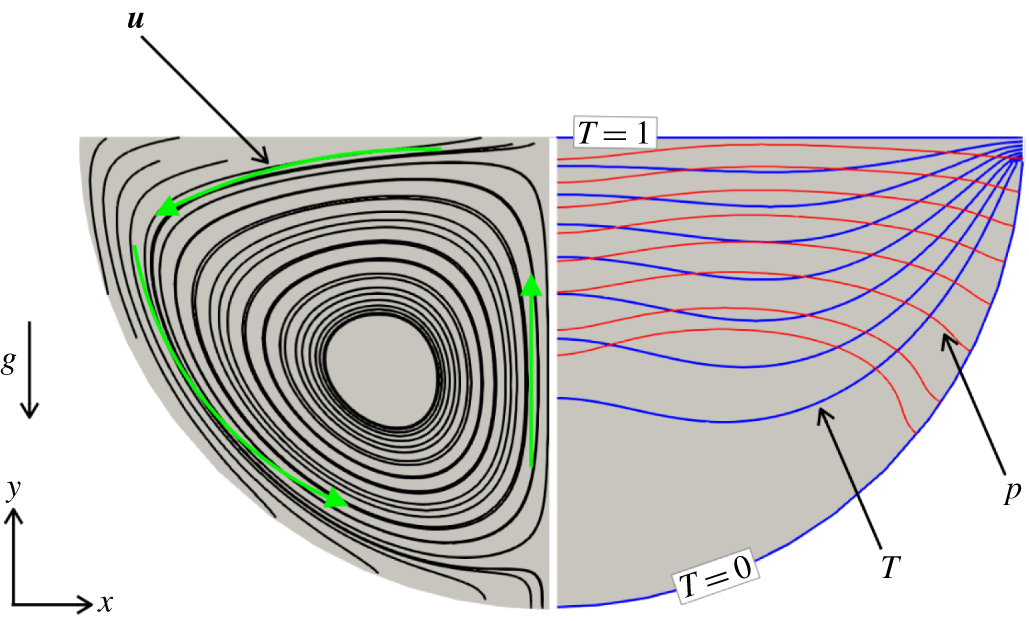
Flow configuration calculated at  $Re=25$ and
 $Ra=10^{4}$. On the left-hand side, the streamlines are in black; on the right-hand side, the isobars are in red and the isotherms in blue. While the convection is initiated by the baroclinic imbalance near the corners, where isobars and isotherms intersect, the rolls result from the return flow generated in the middle, where the jets initiated opposite corners meet.

The first physical ingredient in it is the source of buoyancy. Unlike configurations of the Rayleigh–Bénard type, the stratification itself is not a direct source of instability, as the hot – hence lighter – fluid is fed at the top surface of the pool, while the cold fluid is located at the bottom near the solidification front. Instead, the convection originates from the shape of the isothermal solidification front. Isotherms near it intersect isobars that are mostly horizontal in the bulk but curved near the boundaries (see figure 1). Consequently, the pressure forces cannot oppose the fall of heavy fluid along the boundary and a fluid motion must exist, no matter how small the temperature difference between the hot and the cold boundaries. Barotropic buoyancy sources of this kind are mostly studied in the context of oceans and atmospheres, where the misalignment of density and pressure gradients stems from the pressure contribution of the centrifugal forces due to planetary rotation (Hart Reference Hart1979; Pierrehumbert & Swanson Reference Pierrehumbert and Swanson1995). Nevertheless, the simplest manifestation of baroclinic imbalance is obtained by tilting the plane configuration of the Rayleigh–Bénard problem away from the horizontal position. In an infinite geometry, a flow along the tilted direction is driven by the temperature gradient. At low tilt angles, the base convective flow destabilises to transversal disturbances under the form of non-oscillating rolls at low Prandtl number and travelling waves at high Prandtl number (the Prandtl number  $Pr=\unicode[STIX]{x1D708}/\unicode[STIX]{x1D6FC}$ is the ratio of viscosity
 $\unicode[STIX]{x1D708}$ to thermal diffusivity
 $\unicode[STIX]{x1D6FC}$). At higher tilts, longitudinal rolls dominate (Hart Reference Hart1971; Korpela Reference Korpela1974). While the saturated state may involve nonlinear interaction between transverse and longitudinal modes if their respective critical Rayleigh numbers are close to each other, the travelling wave is by contrast always subject to a secondary instability and not observable (Fujimura & Kelly Reference Fujimura and Kelly1993).
The second ingredient is the through-flow fed in at the upper boundary of the cavity and escaping at the lower boundary through solidification. Through-flows are found in two types of mixed convection problems of some relevance to our configuration: at the boundary of a heated cavity (Papanicolaou & Jaluria Reference Papanicolaou and Jaluria1992) or through a heated conduit (see Jaluria (Reference Jaluria1980) and Kelly (Reference Kelly1994) for reviews), whether a pipe (Shome & Jensen Reference Shome and Jensen1995), a duct (Nicolas, Luijkx & Platten Reference Nicolas, Luijkx and Platten2000) or a channel (Gage & Reid Reference Gage and Reid1968). In all conduit configurations, the shear associated with the through-flow acts as a source of instability. For example, in channels, Tollmien–Schlichting waves are favoured in this way (Schmid & Henningson Reference Schmid and Henningson2001) and the mixed convection patterns result from a competition between buoyancy-driven and hydrodynamically driven instabilities. Whether one or the other dominates depends on the ratios of buoyancy and inertia to viscous forces, respectively measured by the Rayleigh number  $Ra=\unicode[STIX]{x1D6FD}g\unicode[STIX]{x0394}Th^{3}/(\unicode[STIX]{x1D708}\unicode[STIX]{x1D6FC})$ and the Reynolds number
 $Re=U_{0}h/\unicode[STIX]{x1D708}$ (
 $\unicode[STIX]{x1D6FD}$,
 $\unicode[STIX]{x0394}T$,
 $h$,
 $g$,
 $U_{0}$ are the fluid’s thermal expansion coefficient, the temperature difference between boundaries, the domain diameter, gravitational acceleration and the fluid inlet velocity). In the simplest configuration of the Rayleigh–Bénard–Poiseuille problem, transversal rolls dominate at low Reynolds numbers while Tollmien–Schlichting waves characteristic of the Poiseuille flow problem dominate for
 $Re>140$ (Fujimura & Kelly Reference Fujimura and Kelly1995). In rectangular cavities, by contrast, natural convection sets in through an oscillatory mode if the hot wall is located on the side (Briggs & Jones Reference Briggs and Jones1985). The first unstable mode remains oscillatory when mixed convection is introduced with a through-flow along the top wall. It sets in through a ‘rolling pad’ instability for a sufficiently high Richardson number,
 $Gr/Re^{2}$, where the Reynolds number is based on the through-flow and
 $Gr=Ra/Pr$ is the Grashof number. Hence, the through-flow tends to suppress convection (Papanicolaou & Jaluria Reference Papanicolaou and Jaluria1992). This configuration bears important similarities with the problem we are considering, in that isotherms and isobars are not aligned and the thermal instability is damped by a through-flow. In both configurations, the base temperature gradient induces a stable stratification, so convection does not ensue from a Rayleigh–Bénard instability. Nevertheless, the shape of the boundaries differs considerably between the two problems and the through-flow is only local in the work by Papanicolaou & Jaluria (Reference Papanicolaou and Jaluria1992).
Indeed, a specifically interesting aspect of the cavity configuration is that, during continuous casting, the accumulating solid phase at the solidification front is continuously pulled downward, so the lower boundary remains at a constant position. This feature of the process is modelled by means of a porous boundary condition accounting for the mass flux from the liquid to the solid phase, as proposed by Flood & Davidson (Reference Flood and Davidson1994). As such, the through-flow lacks the shear responsible for the hydrodynamic part of the instability in other mixed convection problems, such as the Rayleigh–Bénard–Poiseuille problem, and mainly acts to suppress the base convective flow. The second specificity is that, unlike most other problems of mixed convection, the source of buoyancy is purely baroclinic and not due to an unstable stratification (see figure 1 for the flow configuration). While a background shear can inhibit baroclinic instabilities in open flows (James Reference James1987), the instabilities arising from the interaction of the uniform flow with baroclinic buoyancy in the confined fluid domain we are considering are not known. Because of these specificities, the problem of a heated flow through a cavity may possess a very different phenomenology to that encountered in the problems involving mixed convection discussed above, even though they share some of their ingredients. As such, the convective patterns, whether they are steady or not, and the nature of the bifurcation associated with their onset are not known, despite their central role in solidification problems.
The purpose of this work is precisely to identify both the mechanisms governing the stability of a generic flow supporting this phenomenology and the actual flow that ensues. The minimal geometry with all the necessary ingredients for this purpose was first proposed by Flood & Davidson (Reference Flood and Davidson1994). It consists of a pool with a hot isothermal rigid free-slip upper boundary supporting a uniform inflow and a cold isothermal semicircular solid wall representing the solidification front at the bottom. The stable stratification avoids the complication of mechanisms associated with unstably stratified flows, even though these could occur in some solidification problems depending on the nature of the alloys being solidified (Kuznetsov Reference Kuznetsov1997). For simplicity, the domain shall be assumed infinitely extended in the third direction. We tackle the problem numerically, with both linear stability analysis (LSA) and direct numerical simulations (DNS) based on a combination of the spectral-element method and Fourier-spectral discretisation in the invariant direction. This choice of methodology offers the necessary flexibility to deal with the non-trivial shape of the boundary while retaining the numerical precision of spectral methods (Canuto et al. Reference Canuto, Hussaini, Quarteroni and Zhang1988; Karniadakis & Sherwin Reference Karniadakis and Sherwin1999). We shall seek answers to the following questions:
(i) What is the nature of the base flow?
(ii) In which conditions is this flow stable?
(iii) What is the topology and nature (oscillatory or not) of the unstable mode?
(iv) What is the nature of the bifurcation at the onset of the instability?
After the mathematical definition of the problem and governing equations in § 2, we shall provide the details of the numerical methods we use and of their validation (§ 3). We shall then determine the base flow by means of two-dimensional DNS in the vertical plane (§ 4) and assess its stability to infinitesimal three-dimensional perturbations through LSA (§ 5). Three-dimensional DNS of the flow near the onset of stability shall provide a validation for the LSA approach and indicate whether the saturated state can be inferred from it. The relevance of the LSA approach shall be further validated by seeking the nature of the bifurcation by means of a Stuart–Landau analysis (Sheard, Thompson & Hourigan Reference Sheard, Thompson and Hourigan2004) in § 6. Finally, concluding remarks are presented in § 7.
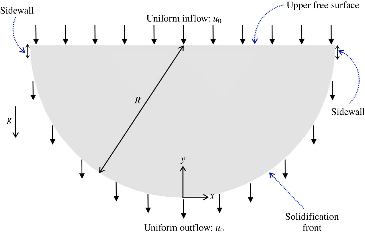
The semicylindrical geometry with the upper free surface, the sidewalls, and the solidification front. The fluid enters at the top and exits through the solidification front with vertical velocity  $u_{0}$.

2 Problem formulation
2.1 Configuration and flow equations
The problem is mostly modelled as proposed by Flood & Davidson (Reference Flood and Davidson1994). We consider a stably stratified flow in a cavity with an upper free surface where the hot fluid is fed in and with a cold porous lower boundary (representing a solidification front), as sketched in figure 2. The cavity is made of a semicircular lower boundary representing the actual front, two adiabatic sidewalls and is considered infinitely extended in the third direction ( $\boldsymbol{e}_{z}$). Since we focus on the convective mechanisms, detailed solidification mechanisms are not modelled. As such, the fluid in the cavity is assumed to remain in a single liquid phase. The fluid is assumed to be Newtonian, incompressible, of density
 $\unicode[STIX]{x1D70C}_{0}$ at a reference temperature
 $T_{0}$, viscosity
 $\unicode[STIX]{x1D708}$, thermal diffusivity
 $\unicode[STIX]{x1D6FC}$, and thermal expansion coefficient
 $\unicode[STIX]{x1D6FD}$. Further considering that temperature gradients remain moderate, the fluid’s motion is described under the Boussinesq approximation (Chandrasekhar Reference Chandrasekhar1968) and the dynamical equations take the non-dimensional form
 $$\begin{eqnarray}\displaystyle & \displaystyle \frac{\unicode[STIX]{x2202}\boldsymbol{u}}{\unicode[STIX]{x2202}t}+(\boldsymbol{u}\boldsymbol{\cdot }\unicode[STIX]{x1D735})\boldsymbol{u}+\unicode[STIX]{x1D735}p=RaPrT\boldsymbol{e}_{y}+Pr\unicode[STIX]{x1D6FB}^{2}\boldsymbol{u}, & \displaystyle\end{eqnarray}$$
 $$\begin{eqnarray}\displaystyle & \displaystyle \frac{\unicode[STIX]{x2202}T}{\unicode[STIX]{x2202}t}+(\boldsymbol{u}\boldsymbol{\cdot }\unicode[STIX]{x1D735})T=\unicode[STIX]{x1D6FB}^{2}T, & \displaystyle\end{eqnarray}$$
 $$\begin{eqnarray}\displaystyle & \displaystyle \unicode[STIX]{x1D735}\boldsymbol{\cdot }\boldsymbol{u}=0, & \displaystyle\end{eqnarray}$$
where  $\boldsymbol{u}=(u,v,w)$ is the velocity vector,
 $t$ the time,
 $p$ the modified pressure including the buoyancy term accounting for the reference temperature (Chandrasekhar Reference Chandrasekhar1968; Tritton Reference Tritton1988) and
 $\boldsymbol{g}=-g\boldsymbol{e}_{y}$ is the gravitational acceleration. These equations are obtained by normalising lengths by the radius of the semicylindrical pool
 $R$, velocities by
 $\unicode[STIX]{x1D6FC}/R$, time by
 $R^{2}/\unicode[STIX]{x1D6FC}$, pressure by
 $\unicode[STIX]{x1D70C}_{0}(\unicode[STIX]{x1D6FC}/R)^{2}$ and temperature by
 $\unicode[STIX]{x0394}T$. Here,
 $\unicode[STIX]{x0394}T$ is the temperature difference between the hot upper free surface and the cold solidification front at the lower boundary. Note that the term involving the reference temperature is absorbed in the pressure gradient through the modified definition of pressure. The Prandtl number,
 $Pr=\unicode[STIX]{x1D708}/\unicode[STIX]{x1D6FC}$, is fixed to
 $0.02$, a value typical of liquid metals in continuous casting processes. The Rayleigh number
 $Ra$ is defined as
 $$\begin{eqnarray}Ra=\frac{\unicode[STIX]{x1D6FD}g\unicode[STIX]{x0394}TR^{3}}{\unicode[STIX]{x1D708}\unicode[STIX]{x1D6FC}}.\end{eqnarray}$$
The upper boundary at  $y=1$ is modelled as a rigid free surface (standard free-slip boundary condition), where incoming fluid at an imposed temperature
 $\unicode[STIX]{x0394}T$ is poured with a homogeneous spatial distribution. This is expressed with three boundary conditions:
 $$\begin{eqnarray}\displaystyle \frac{\unicode[STIX]{x2202}}{\unicode[STIX]{x2202}y}\boldsymbol{u}\times \boldsymbol{e}_{y}=0,\quad \boldsymbol{u}\boldsymbol{\cdot }\boldsymbol{e}_{y}=RePr,\quad T(y=1)=1, & & \displaystyle\end{eqnarray}$$
where the mass flux Reynolds number  $Re$ is based on the dimensional feeding velocity
 $u_{0}$. In a continuous casting process, this velocity would correspond to the casting speed (Flood & Davidson Reference Flood and Davidson1994):
 $$\begin{eqnarray}Re=\frac{u_{0}R}{\unicode[STIX]{x1D708}}.\end{eqnarray}$$
Thus,  $Re=0$ corresponds to zero net mass flux, i.e. no fluid crosses through the boundaries of the semicylindrical pool, while
 $Re\neq 0$ corresponds to non-zero net mass flux, i.e. the fluid enters and leaves the domain uniformly through the upper and lower surfaces as in Flood & Davidson (Reference Flood and Davidson1994). The incoming mass flux is exactly cancelled by the flux of fluid being solidified and pulled at the solid lower boundary
 $S$, where solidification imposes the reference temperature:
 $$\begin{eqnarray}\displaystyle \boldsymbol{u}_{S}\times \boldsymbol{e}_{y}=0,\quad \boldsymbol{u}_{S}\boldsymbol{\cdot }\boldsymbol{e}_{y}=RePr,\quad T(y=0)=0. & & \displaystyle\end{eqnarray}$$
The kinematic condition expresses that the fluid flows vertically downwards through the otherwise no-slip but porous lower boundary. Note that the slight differences between the definitions of the Rayleigh and Reynolds numbers given in the introduction and the ones given in this section reflect the difference between the geometries discussed there and the specific one we are considering in this paper. To ensure consistent boundary conditions for the temperature field at the corners of the domain, short sidewalls of  $0.05R$ in height separate the upper and the lower boundaries. Impermeable, no-slip boundary conditions for the velocity field and an insulating boundary condition for the temperature field are imposed at these sidewalls. In a real casting process, these walls represent the mould. Finally, the infinite extension of the domain in the third direction
 $\boldsymbol{e}_{z}$ is represented by periodic boundary conditions for the velocity and temperature fields.
2.2 Linear stability analysis
The system admits steady base solutions that are invariant along  $\boldsymbol{e}_{z}$, similar to those found by Flood & Davidson (Reference Flood and Davidson1994) (see the detailed topology of these solutions in § 4). These may, however, be unstable to three-dimensional perturbations. Hence, we shall detect the corresponding bifurcation by analysing the stability of the base two-dimensional flow to infinitesimal three-dimensional perturbations. As such, velocity, pressure and temperature fields are decomposed into the two-dimensional base flow and an infinitesimal three-dimensional perturbation, as
 $$\begin{eqnarray}\displaystyle & \displaystyle \boldsymbol{u}(x,y,z,t)=\boldsymbol{U}(x,y)+\boldsymbol{u}^{\prime }(x,y,z,t), & \displaystyle\end{eqnarray}$$
 $$\begin{eqnarray}\displaystyle & \displaystyle T(x,y,z,t)=\bar{T}(x,y)+T^{\prime }(x,y,z,t), & \displaystyle\end{eqnarray}$$
 $$\begin{eqnarray}\displaystyle & \displaystyle p(x,y,z,t)=P(x,y)+p^{\prime }(x,y,z,t). & \displaystyle\end{eqnarray}$$
Substituting (2.8)–(2.10) into (2.1)–(2.3) and retaining first-order terms only yields the linearised equations governing the evolution of infinitesimal perturbations:
 $$\begin{eqnarray}\displaystyle & \displaystyle \frac{\unicode[STIX]{x2202}\boldsymbol{u}^{\prime }}{\unicode[STIX]{x2202}t}+(\boldsymbol{u}^{\prime }\boldsymbol{\cdot }\unicode[STIX]{x1D735})\boldsymbol{U}+(\boldsymbol{U}\boldsymbol{\cdot }\unicode[STIX]{x1D735})\boldsymbol{u}^{\prime }+\unicode[STIX]{x1D735}p^{\prime }=RaPrT^{\prime }\boldsymbol{e}_{y}+Pr\unicode[STIX]{x1D6FB}^{2}\boldsymbol{u}^{\prime }, & \displaystyle\end{eqnarray}$$
 $$\begin{eqnarray}\displaystyle & \displaystyle \frac{\unicode[STIX]{x2202}T^{\prime }}{\unicode[STIX]{x2202}t}+(\boldsymbol{u}^{\prime }\boldsymbol{\cdot }\unicode[STIX]{x1D735})\bar{T}+\boldsymbol{U}\boldsymbol{\cdot }\unicode[STIX]{x1D735}T^{\prime }=\unicode[STIX]{x1D6FB}^{2}T^{\prime }, & \displaystyle\end{eqnarray}$$
 $$\begin{eqnarray}\displaystyle & \displaystyle \unicode[STIX]{x1D735}\boldsymbol{\cdot }\boldsymbol{u}^{\prime }=0. & \displaystyle\end{eqnarray}$$
The base flow  $(\boldsymbol{U},\bar{T},P)$ satisfies the same boundary conditions as the main variables
 $(\boldsymbol{u},T,p)$ so that the perturbation variables satisfy the homogeneous counterpart of the boundary conditions associated with the base flow. Since the base flow is invariant along
 $\boldsymbol{e}_{z}$, the general perturbation may be decomposed into normal Fourier modes as
 $$\begin{eqnarray}\boldsymbol{q}^{\prime }(x,y,z,t)=\mathop{\sum }_{k=-\infty }^{\infty }\hat{\boldsymbol{q}}(x,y,t)\text{e}^{\text{i}kz},\end{eqnarray}$$
where  $\boldsymbol{q}^{\prime }=(\boldsymbol{u}^{\prime },T^{\prime },p^{\prime })$ contains all perturbation fields and
 $k$ is the wavenumber along the homogeneous direction
 $\boldsymbol{e}_{z}$. Further, the absence of the third component of the velocity field in the base flow allows a single phase of the complex Fourier mode to be considered, following Barkley & Henderson (Reference Barkley and Henderson1996) and others (Barkley, Gomes & Henderson Reference Barkley, Gomes and Henderson2002; Sapardi et al. Reference Sapardi, Hussam, Pothérat and Sheard2017). The two-dimensionality of the base allows us to reduce the three-dimensional perturbation field to a family of two-dimensional fields parametrised by wavenumber
 $k$ and computed on the same two-dimensional domain as the base flow.
The LSA equations shall be solved by means of a time-stepper method: defining a linear time evolution operator  ${\mathcal{A}}(\unicode[STIX]{x1D70F})$ for the time integration of (2.11)–(2.13) over time interval
 $\unicode[STIX]{x1D70F}$ as
 $$\begin{eqnarray}\hat{\boldsymbol{q}}(t+\unicode[STIX]{x1D70F})={\mathcal{A}}(\unicode[STIX]{x1D70F})\hat{\boldsymbol{q}}(t),\end{eqnarray}$$
we solve the eigenvalue problem for operator  ${\mathcal{A}}(\unicode[STIX]{x1D70F})$ as
 $$\begin{eqnarray}{\mathcal{A}}(\unicode[STIX]{x1D70F})\hat{\boldsymbol{q}}_{j}=\unicode[STIX]{x1D707}_{j}\hat{\boldsymbol{q}}_{j}.\end{eqnarray}$$
Here  $\hat{\boldsymbol{q}}_{j}$ denotes the eigenvector of
 ${\mathcal{A}}(\unicode[STIX]{x1D70F})$ corresponding to the complex eigenvalue
 $\unicode[STIX]{x1D707}_{j}$. The growth rate
 $\unicode[STIX]{x1D70E}$ and frequency
 $\unicode[STIX]{x1D714}$ of an eigenmode are related to
 $\unicode[STIX]{x1D707}$ through
 $$\begin{eqnarray}\unicode[STIX]{x1D707}=\exp [(\unicode[STIX]{x1D70E}+\text{i}\unicode[STIX]{x1D714})\unicode[STIX]{x1D70F}],\end{eqnarray}$$
where the subscript is ignored for brevity. Further, equation (2.17) yields
 $$\begin{eqnarray}\unicode[STIX]{x1D70E}=\frac{\ln |\unicode[STIX]{x1D707}|}{\unicode[STIX]{x1D70F}};\quad \unicode[STIX]{x1D714}=\frac{\unicode[STIX]{x1D703}}{\unicode[STIX]{x1D70F}},\end{eqnarray}$$
with  $\unicode[STIX]{x1D707}=|\unicode[STIX]{x1D707}|\text{e}^{\text{i}\unicode[STIX]{x1D703}}$. An instability occurs if
 $\unicode[STIX]{x1D70E}>0$, i.e.
 $|\unicode[STIX]{x1D707}|>1$, while for
 $|\unicode[STIX]{x1D707}|<1$ the corresponding eigenmode is stable. The growing eigenmode may be either oscillatory (
 $\unicode[STIX]{x1D714}\neq 0$) or non-oscillatory (
 $\unicode[STIX]{x1D714}=0$). The smallest Rayleigh number for which at least one wavenumber
 $k$ achieves
 $|\unicode[STIX]{x1D707}|=1$ is the critical Rayleigh number for the onset of instability at a particular value of
 $Re$, which we shall denote as
 $Ra_{c}$.
3 Computational methods
3.1 Numerical set-up
We perform three different types of numerical computations. First, steady two-dimensional solutions obtained using DNS of (2.1)–(2.3) with associated boundary conditions. Two-dimensionality is enforced by setting  $\unicode[STIX]{x2202}/\unicode[STIX]{x2202}z=0$ and
 $w=0$. Second, the LSA of three-dimensional perturbations on the two-dimensional base flow is carried out, by solving the eigenvalue problem set out in § 2.2. This yields the bifurcation points and the structure of the first unstable mode, in the sense of growing
 $Ra$. Third, three-dimensional DNS are performed in weakly sub- and supercritical regimes for two purposes: (1) to assess the relevance of the LSA results and (2) to find the nature of the bifurcation. The latter is obtained by computing the parameters of the Stuart–Landau model from the three-dimensional DNS data, as proposed by Sheard et al. (Reference Sheard, Thompson and Hourigan2004).
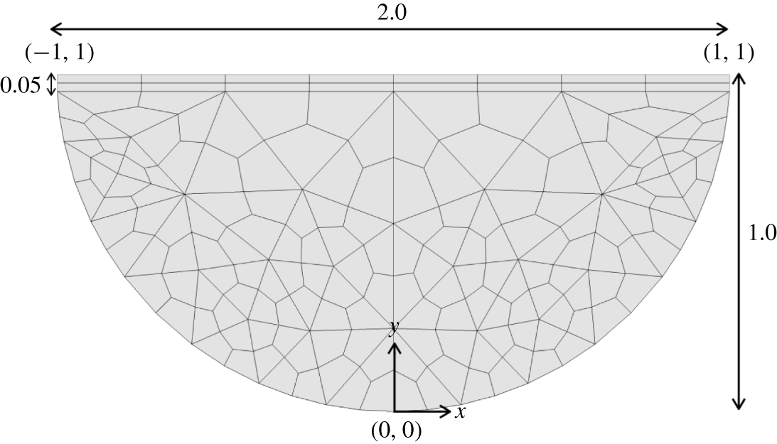
Details of the mesh with polynomial order  $N=1$. The mesh contains 184 quadrilateral elements.

Both the two-dimensional base flow and the evolution of the three-dimensional flow near criticality are obtained by solving (2.1)–(2.3) using spectral-element code Nektar++ (Cantwell et al. Reference Cantwell, Moxey, Comerford, Bolis, Rocco, Mengaldo, Grazia, Yakovlev, Lombard and Ekelschot2015). In the spectral-element approach, the computational domain is partitioned into a mesh of many small subdomains called elements, and the variables are projected within a polynomial basis within each element, as in the finite element method. The specificity of the spectral-element method is that ‘mesh’ refinement is mainly achieved by increasing the order of the polynomial basis ( $p$-refinement) and that polynomials are represented at Gauss–Lobatto points which ensure spectral convergence under
 $p$-refinement. Both two- and three-dimensional DNS are performed on the same spectral-element mesh in the
 $x\text{-}y$ plane. For the three-dimensional simulations, discretisation in the
 $\boldsymbol{e}_{z}$ direction relies on a Fourier-based spectral method. The computational domain extends by
 $2\unicode[STIX]{x03C0}$ along
 $\boldsymbol{e}_{z}$, or equivalently, the lowest Fourier mode in the spectral discretisation is always
 $k=1$. Figure 3 shows the detail of the two-dimensional
 $x\text{-}y$ mesh with polynomial order
 $N=1$, generated using the GMSH package (Geuzaine & Remacle Reference Geuzaine and Remacle2009). The mesh is composed of 184 quadrilateral elements and is structured in the rectangular part of the domain close to the upper free surface up to thickness
 $0.05$, and unstructured in the remaining part of the domain. A vertical line along the
 $y$-axis is imposed to ensure the symmetry of the mesh with respect to that line. At the boundaries, elements are more densely packed than in the bulk, with the ratio between the largest to smallest element’s edge size of four. Time-stepping relies on a third-order implicit–explicit (IMEX) method (Vos et al. Reference Vos, Eskilsson, Bolis, Chun, Kirby and Sherwin2011).
The LSA is conducted with open-source eigenvalue solver DOG (Direct Optimal Growth, Blackburn & Sherwin (Reference Blackburn and Sherwin2004), Pitz, Marxen & Chew (Reference Pitz, Marxen and Chew2017)), based on a time-stepper method with spectral-element discretisation. The linearised equations (2.11)–(2.13) are integrated in time using a third-order backward differentiation scheme (Karniadakis, Israeli & Orszag Reference Karniadakis, Israeli and Orszag1991), with the two-dimensional base flow obtained from the DNS. The leading eigenvalues and eigenmodes are obtained using the iterative process from the method prescribed by Tuckerman & Barkley (Reference Tuckerman and Barkley2000) and Barkley, Blackburn & Sherwin (Reference Barkley, Blackburn and Sherwin2008).
For the two-dimensional DNS, the initial condition is set to  $\boldsymbol{u}=0$,
 $p=0$, and
 $T=y$. The three-dimensional DNS are initiated with the solution obtained for the two-dimensional base flow replicated along
 $\boldsymbol{e}_{z}$, with added white noise of standard deviation
 $0.001$ (as well as
 $0.01$ and
 $0.1$ for
 $Ra<Ra_{c}$ when the bifurcation is subcritical, i.e.
 $Re=100$ and
 $Re=110$).
Cubic spline interpolation of the SCIPY package (Virtanen et al. Reference Virtanen, Gommers, Oliphant, Haberland, Reddy, Cournapeau, Burovski, Peterson, Weckesser and Bright2019) is used to estimate the Rayleigh number that first produces  $\unicode[STIX]{x1D70E}(k)=0$ at different values of
 $k$. This gives the curve for Rayleigh number versus
 $k$, whose minimum yields the estimate of the critical Rayleigh number
 $Ra_{c}$ and the critical wavenumber
 $k_{c}$. Again, by cubic spline interpolation, we estimate the value of critical frequency
 $\unicode[STIX]{x1D714}_{c}$ for the corresponding
 $k_{c}$. The resulting uncertainty on
 $Ra_{c}$,
 $k_{c}$ and
 $\unicode[STIX]{x1D714}_{c}$ remains within 0.01 %.
3.2 Code validation
We first validated the DNS code and the linear stability solver DOG for two-dimensional Rayleigh–Bénard convection in a box. At the top and bottom plates, a no-slip boundary condition for the velocity field and a conducting boundary condition for the temperature field are imposed. Periodic boundary conditions are applied at the sidewalls for both the fields. DNS were validated by calculating the Nusselt number
 $$\begin{eqnarray}Nu=\frac{\unicode[STIX]{x1D6FC}{\displaystyle \frac{\unicode[STIX]{x0394}T}{R}}+\langle wT\rangle }{\unicode[STIX]{x1D6FC}{\displaystyle \frac{\unicode[STIX]{x0394}T}{R}}},\end{eqnarray}$$
where  $\langle \rangle$ represents the volume average. Here,
 $Nu$ measures the ratio of the total (convective plus conductive) heat flux to the conductive heat flux. It was computed for
 $Pr=0.71$ and
 $Ra=5000$ in a two-dimensional box and the relative error between the Nusselt number computed from our DNS and that of Clever & Busse (Reference Clever and Busse1974) was 0.09 %. For the LSA, we recovered the known values of the critical Rayleigh number (
 $Ra_{c}=1707.7$) and critical wavenumber (
 $k_{c}=3.116$) found, for instance, in Chandrasekhar (Reference Chandrasekhar1968), to within an uncertainty of 0.002 %. For both DNS and LSA, a rectangular mesh of 100 structured quadrilateral elements with polynomial order
 $N=9$ was used.
3.3 Convergence tests
Since the spectral-element discretisation is only used in the  $x\text{-}y$ plane, we performed a convergence test on the base two-dimensional flows and the eigenvalue problem based on the two-dimensional domain. This test was performed for each value of
 $Re$ we considered throughout this work, both on the DNS and on the leading eigenvalue returned by the LSA at
 $k$ for which
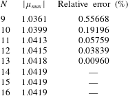
 $\unicode[STIX]{x1D70E}(k)$ is maximum. Table 1 shows an example for the accuracy of the eigenvalue calculations as a function of the polynomial degree
 $N$ for
 $Re=500$, the highest value of
 $Re$ considered in this work. The leading eigenvalue for
 $Ra=2\times 10^{6}$ and
 $k=13$ is real and linearly unstable. We increased
 $N$ until the eigenvalue converged to a precision of five significant figures, which is
 $N=14$ for this case. This way, the same level of precision was achieved for all results presented in this work. The time step was kept constant for all three types of numerical calculations so that the maximum local Courant number
 $C_{max}$ remained below unity and the Courant–Friedrich–Levy condition was strictly satisfied everywhere in the domain, at all time. For instance, at
 $Re=500$,
 $Ra=2\times 10^{6}$ and
 $N=16$, the time step is
 $10^{-6}$, which yields a maximum Courant number of
 $C_{\text{max}}=0.05$.
Dependence of leading eigenvalues on the polynomial order  $N$. Leading eigenvalues computed on the mesh at
 $Re=500$,
 $Ra=2\times 10^{6}$ and
 $k=13$ are provided. The relative error is to the case of the highest polynomial order (
 $N=16$).

Furthermore, some supercritical cases (for example,  $Re=200$ and
 $Ra=10^{6}$) are unstable to time-periodic, two-dimensional perturbations. In these cases, a DNS of the base flow over the entire two-dimensional domain does not converge to the base steady solution. Since the perturbation breaks a symmetry with respect to the
 $x=0$ plane, we found the steady state by performing a DNS on the
 $x\leqslant 0$ half of the domain, implementing symmetry boundary conditions for the velocity (Neumann boundary condition on
 $u$, Dirichlet boundary condition on
 $v$) and the temperature (Neumann boundary condition) at
 $x=0$. The solution over the full domain was then built by symmetry (Mao & Blackburn Reference Mao and Blackburn2014). We checked that the relative error in the magnitude of the most dominant mode for
 $Re=200$,
 $Ra=10^{5}$ and
 $k=7$ obtained from LSA on base flows calculated on the full domain and the half-domain was less than 0.01 %. Thus, the use of half-domain calculation for the base flow is justified and also computationally cheaper.
For the three-dimensional DNS, the dependence on the number of Fourier modes  $N_{f}$ was tested by computing the total kinetic energy of the three-dimensional flow over the entire domain. The relative error in the kinetic energy of the supercritical steady state at
 $Re=200$ and
 $Ra=1.1\times 10^{5}$ between computations at
 $N_{f}=32$ and
 $N_{f}=64$ was 0.01 %. Similar results were obtained for other values of
 $Re$, and thus 32 Fourier modes were employed for all cases. Note that the three-dimensional simulations are performed only up to
 $Re=200$, as the simulations for higher values of
 $Re$ become prohibitively expensive. A summary of all cases investigated is provided in table 5.
4 Two-dimensional base flows
4.1 Dynamics of base flow with zero net mass flux ( $Re=0$)

To perform a LSA, we first need to obtain the two-dimensional base flow. We first focus on the behaviour of two-dimensional base flow with zero net mass flux. Figure 4 displays the density plots of the temperature field and the velocity vector field  $\boldsymbol{u}$ in the
 $x\text{-}y$ plane for
 $Re=0$ and
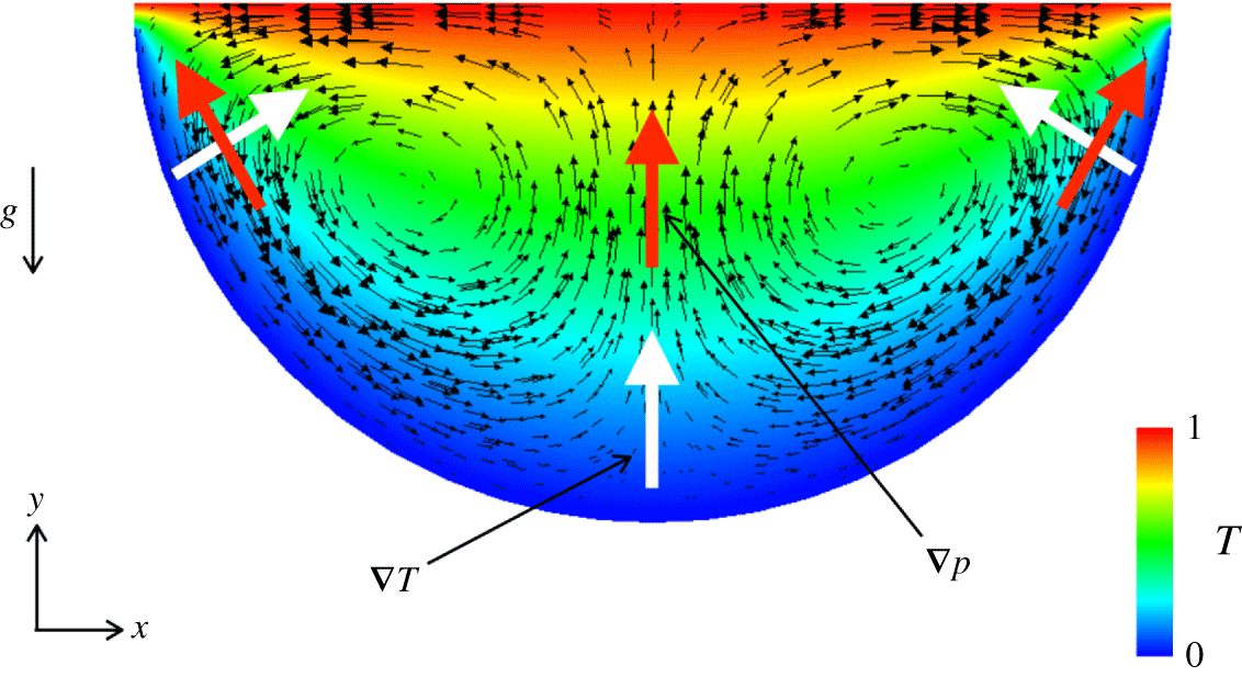
 $Ra=1$. Despite a ‘stable’ stratification (i.e. the light fluid is mostly on the top of the heavy one), we observe prominent convective rolls. This motion is driven by the misalignment of the pressure gradient and the temperature gradient, which generates a baroclinic imbalance. This effect is best seen by considering an equilibrium state and the small displacement of a fluid particle along an isothermal line. In a Rayleigh–Bénard configuration, isobars and isotherms are aligned, so no change in either buoyancy or pressure forces on the fluid particle occurs as a result of the displacement. If, on the other hand, isobars and isotherms are not aligned, as in the present configuration (and if the isobars are reasonably parallel), the displacement results in a variation of pressure forces in the direction normal to the isobar. Since the displacement takes place along an isotherm, the excess or deficit in pressure forces is not compensated by a variation in buoyancy forces and a motion must take place for viscous forces to restore equilibrium. Near the semicircular boundary of the domain, the temperature gradient is radial, whereas the pressure gradient (dominated by buoyancy) is tilted. While these directions coincide near the centre of the domain (around
 $x=0$), the angle they form increases to a maximum near the sidewalls. At these locations, the imbalance is maximum and drives a strong downward jet along the circular boundary. The rolls form as a result of the left and right jets meeting at where the flow returns. This form of baroclinic imbalance drives a non-zero base flow, even at arbitrary low-temperature gradients. It is noteworthy that this mechanism is a simpler form of the classical baroclinic imbalance in models incorporating an explicit temperature dependence of the density. In these models, the imbalance appears explicitly in the dimensional vorticity equation, where the curl of the pressure term yields a vorticity source term proportional to the baroclinic vector
 $1/\unicode[STIX]{x1D70C}(T)^{2}\unicode[STIX]{x1D735}\unicode[STIX]{x1D70C}(T)\times \unicode[STIX]{x1D735}p$ (Vallis Reference Vallis2006), and where the density gradient is
 $\unicode[STIX]{x1D735}\unicode[STIX]{x1D70C}(T)=-\unicode[STIX]{x1D735}T/\unicode[STIX]{x1D6FD}$ in dimensional variables. Again, in Rayleigh–Bénard configurations the gradients of vorticity and pressure are aligned, so the baroclinic vector is zero. In the semicircular cavity, by contrast, the baroclinic vector is maximum near the corner and drives a jet along the wall in exactly the same way as in the model we are using.
Two-dimensional base flow at  $Re=0$ and
 $Ra=1$. The pressure gradient (
 $\unicode[STIX]{x1D735}p$) and the temperature gradient (
 $\unicode[STIX]{x1D735}T$) are indicated by red and white arrows, respectively. These gradients form an angle at the upper corners, which results in a baroclinic imbalance. In models with explicit dependence of the density on the temperature, the density gradient is related to the temperature gradient as
 $\unicode[STIX]{x1D735}\unicode[STIX]{x1D70C}=-\unicode[STIX]{x1D6FD}^{-1}\unicode[STIX]{x1D735}T$ in dimensional variables. Note that in this example, the modified pressure is predominantly determined by the buoyancy, as it includes the buoyancy term corresponding to the reference temperature.

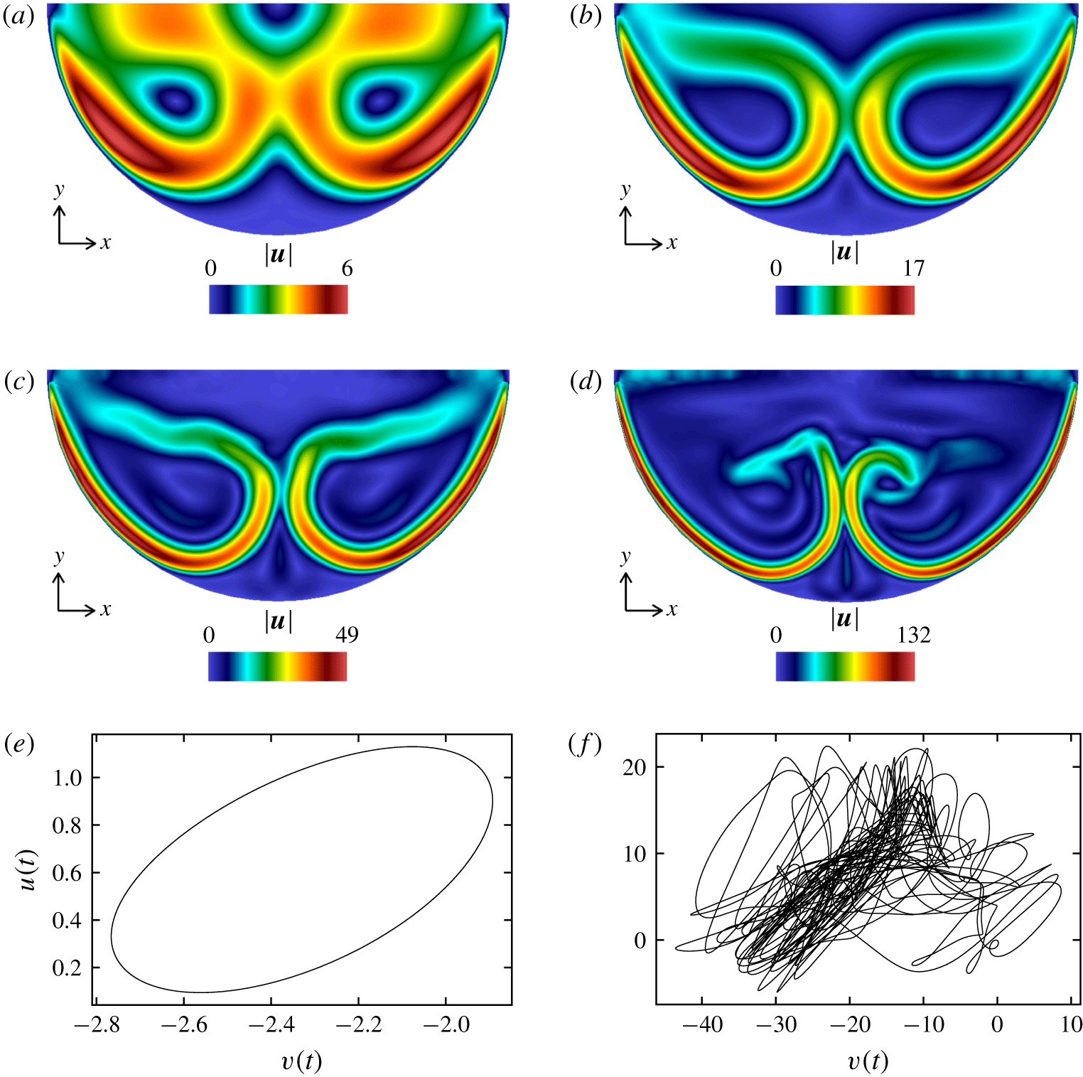
Two-dimensional base flow with zero net mass flux ( $Re=0$) at (a)
 $Ra=10^{4}$; (b)
 $Ra=10^{5}$; (c)
 $Ra=10^{6}$; and (d)
 $Ra=10^{7}$. Colours represent the magnitude of the velocity field. Panels (e and f) display Lissajous graphs in the
 $(u,v)$ plane for
 $Ra=10^{6}$ and
 $Ra=10^{7}$ measured at
 $(x,y)=(-0.5,0.6)$, respectively exhibiting periodic and chaotic states.

Interestingly, if the curvature of the lower boundary was continuously decreased to zero, the angle between the temperature and pressure gradient would progressively decrease to zero, too. In the limit of a flat lower boundary, the Rayleigh–Bénard configuration would be recovered in a channel of height determined by the sidewalls, even though these would be pushed to infinity. However, the stratification would be stable and since the baroclinic imbalance (and also the baroclinic vector) would cancel out in this limit, the base flow would be still and stable, with a linear temperature gradient in the bulk.
We now gradually increase the Rayleigh number from  $Ra=10^{4}$ to
 $Ra=10^{7}$ with
 $Re=0$. As expected, the velocity field strengthens at the wall with the increase in Rayleigh number, since the intensity of the temperature gradient in the baroclinic vector increases (see figure 5a–d). While the two-dimensional solution remains steady for
 $Ra=10^{4}$ and
 $Ra=10^{5}$, it becomes time-periodic for
 $Ra=10^{6}$ and chaotic for
 $Ra=10^{7}$. The periodic and chaotic nature of the solutions for
 $Ra=10^{6}$ and
 $Ra=10^{7}$ are illustrated by the Lissajous graphs of the two components of velocities in figures 5(e) and 5(f).
4.2 Base solution with non-zero mass flux ($Re>0$)

One of the key ingredients in the problem we consider is the through-flow. To illustrate its effect on the base flow, we computed the two-dimensional base flows for a range of Reynolds numbers from 0 to 200, at a fixed value of  $Ra$ of
 $10^{4}$ (for the purpose of seeking the critical Rayleigh number for the linear stability, the base flow will have to be recalculated every time either
 $Ra$ or
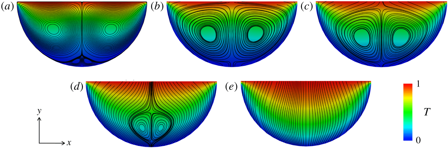
 $Re$ is changed). Figure 6 shows the streamlines of the velocity field and the density plots of the temperature field for the two-dimensional base flow. At
 $Re=0$, the flow consists of the pair of primary vortices and the pair of secondary vortices which are located at the bottom of the cavity, as discussed in the previous section. At low values of
 $Re$ (
 $Re=25$), the primary vortices are slightly displaced downwards and secondary vortices are suppressed under the combined action of the through-flow and the confinement at the lower boundary. The size of the primary vortices increases as a result, and the convection associated with them is slightly enhanced. However, with a further increase in
 $Re$, the same mechanism incurs a suppression of the primary vortices from the top and a reduction of their size. At
 $Re=200$, the primary vortices have completely disappeared. Thus, the through-flow enhances convection at low Reynolds numbers (below 25, in the set of Reynolds numbers we explored), but suppresses it at higher Reynolds numbers.
Streamlines of the steady two-dimensional base flow and temperature field for  $Ra=10^{4}$ at (a)
 $Re=0$; (b)
 $Re=25$; (c)
 $Re=50$; (d)
 $Re=100$; and (e)
 $Re=200$.

4.3 Vertical heat flux
The efficiency of the convection is estimated by quantifying the vertical heat flux. For this purpose, we compute the Nusselt number at the inlet of the cavity defined as
 $$\begin{eqnarray}Nu=\frac{-\left\langle \left({\displaystyle \frac{\unicode[STIX]{x2202}T}{\unicode[STIX]{x2202}y}}\right)_{y=1}\right\rangle _{Convective}+(vT)_{y=1}}{-\left\langle \left({\displaystyle \frac{\unicode[STIX]{x2202}T}{\unicode[STIX]{x2202}y}}\right)_{y=1}\right\rangle _{Conductive}+(vT)_{y=1}},\end{eqnarray}$$
and analyse its variations with the Rayleigh number for several fixed values of  $Re$. Here the reference conductive state is chosen as a uniform downward flow at non-dimensional velocity
 $RePr$, without rolls. This way, the Nusselt number in (4.1) measures the enhancement of heat transfer due to the convective flow inside the cavity and not that due to the average downward fluid motion. The temperature distribution for this reference state is obtained by solving the steady advection-diffusion equation
 $$\begin{eqnarray}\unicode[STIX]{x1D6FB}^{2}T-(RePr\boldsymbol{e}_{y}\boldsymbol{\cdot }\unicode[STIX]{x1D735})T=0,\end{eqnarray}$$
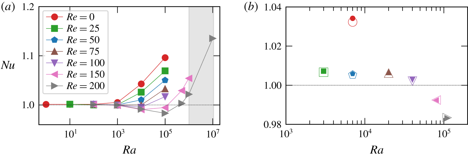
with the same boundary conditions for the temperature as for the base flow (2.5) and (2.7). The variations of  $Nu$ with the Rayleigh number for the two-dimensional base flow are shown in figure 7(a). For
 $Re=0$, the Nusselt number monotonically increases with
 $Ra$. By contrast, for
 $Re\neq 0$,
 $Nu$ first decreases before reaching a minimum, and it goes below unity for
 $Re=75$ to
 $Re=200$. The decrease of
 $Nu$ below unity occurs as the two rolls form and gain in intensity. As they do so, they redistribute heat laterally in the upper part of the pool. As they grow in size, they do so ever closer to the top boundary and oppose the downward temperature gradient near the corners and hence the heat flux through the upper boundary. When the convective rolls have grown to occupy the entire cavity, however, their shape does not evolve any more as
 $Ra$ is further increased. In this regime, the heat flux near the corners saturates and the main effect of the rolls is to convey cold fluid upwards near
 $x=0$. The cooling of the region near the upper boundary that ensues leads
 $Nu$ to increase again and soon exceed unity. There are relatively few instances where convection reduces rather than enhances heat transfer (i.e.
 $Nu<1$). It has, for example, been observed in the Rayleigh–Bénard convection of homeotropically aligned nematic liquid crystal (Thomas, Pesch & Ahlers Reference Thomas, Pesch and Ahlers1998).
Nusselt number  $Nu$ calculated at the inlet. Panel (a) shows two-dimensional base flow for various values of
 $Ra$. The shaded region represents the unsteady case. Panel (b) shows a comparison between
 $Nu$ for two-dimensional (represented by solid symbols) and three-dimensional (represented by hollow symbols) DNS at the same value of the Rayleigh number. Points are obtained near criticality (hence, for different values of
 $Re$).

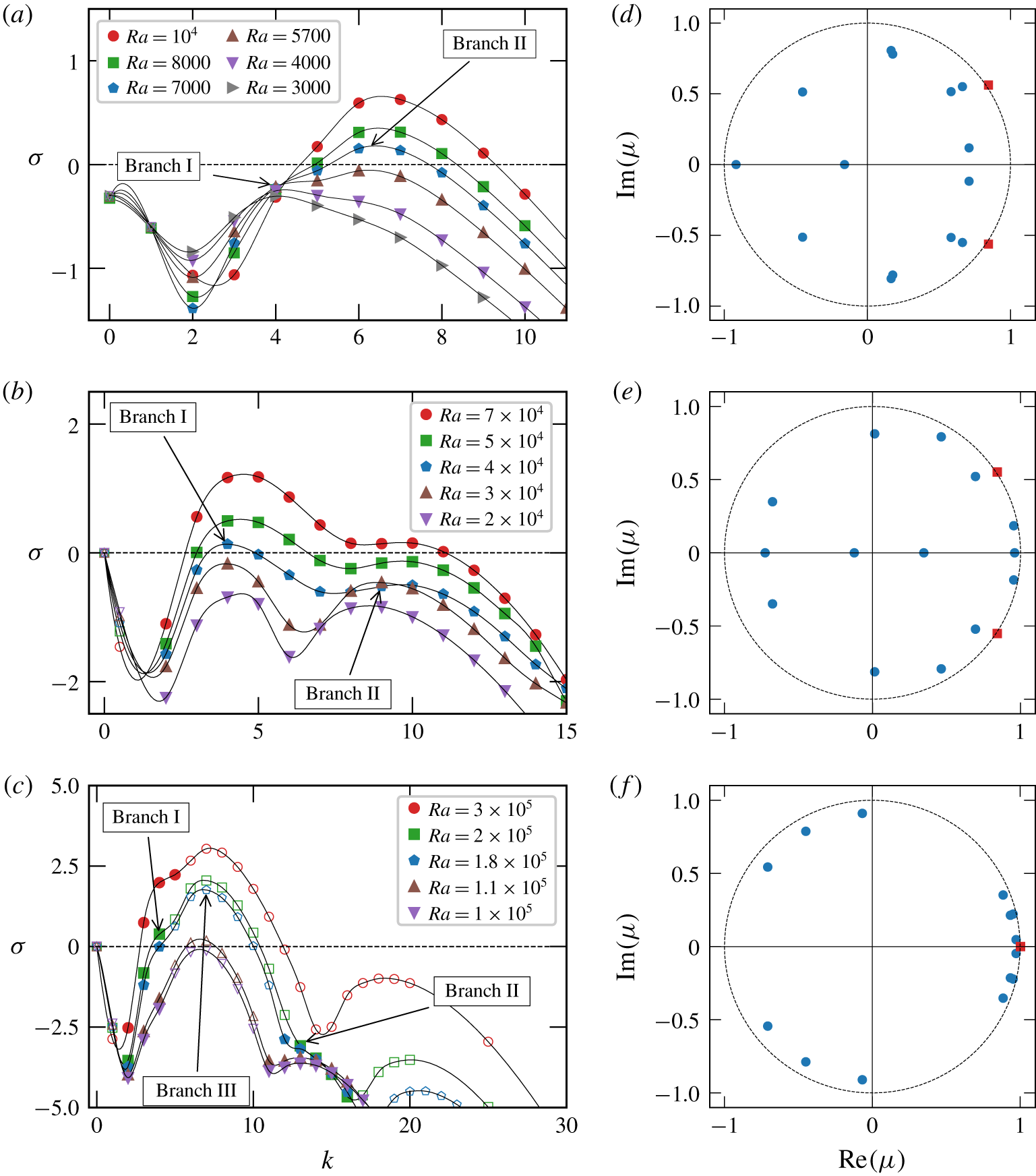
Growth rates of leading eigenmodes as functions of the wavenumber  $k$ for (a)
 $Re=0$ and
 $Ra\leqslant 10^{4}$; (b)
 $Re=100$ and
 $Ra\leqslant 7\times 10^{4}$; and (c)
 $Re=200$ and
 $Ra\leqslant 3\times 10^{5}$. Solid symbols represent real leading eigenvalues, while hollow symbols represent complex-conjugate pairs of non-real leading eigenvalues. Eigenvalue spectra for marginally supercritical cases for (d)
 $Re=0$,
 $Ra=7\times 10^{3}$ and
 $k=6$; (e)
 $Re=100$,
 $Ra=4\times 10^{4}$ and
 $k=4$ and (f)
 $Re=200$,
 $Ra=1.1\times 10^{5}$ and
 $k=7$. Symbols: ●, blue, stable eigenvalues; ▪, red, the first unstable eigenvalue.

5 Stability analysis
5.1 Growth rates and eigenvalue spectra
We now turn to the linear stability of the steady two-dimensional states found in § 4. We start by analysing the dependence of the perturbation growth  $\unicode[STIX]{x1D70E}$ on the Rayleigh number
 $Ra$, wavenumber
 $k$ and mass flux Reynolds number
 $Re$. Figure 8(a–c) shows the growth rate
 $\unicode[STIX]{x1D70E}$ as a function of wavenumber
 $k$ for
 $Re=0$, 100 and 200. For a particular value of
 $Re$, the growth rate
 $\unicode[STIX]{x1D70E}(k)$ is computed for a range of Rayleigh numbers until supercritical regimes are encountered. Figure 8(d–f) shows the eigenvalue spectra for
 $Re$ (corresponding to figure 8a–c) near to the onset of instability, in marginally supercritical regime. For
 $Re=0$, all eigenmodes are oscillatory (
 $\unicode[STIX]{x1D714}\neq 0$) over the entire range of values of
 $Ra$ we investigated. At low wavenumber
 $k\simeq 4$, a local maximum in
 $\unicode[STIX]{x1D70E}(k)$ is observed. We denote the set of eigenvectors forming this maximum as ‘branch I’. These remain stable for all values of
 $Ra$ we investigated. A second, absolute maximum exists around
 $k\simeq 6$ and we shall label the corresponding set of modes as ‘branch II’. The mode associated with this maximum becomes unstable for
 $Ra=7\times 10^{3}$. The corresponding pair of complex conjugate eigenvalues are shown in figure 8(d) as they cross the unit circle that separates stable from unstable eigenmodes. Branches I and II (as well as branch III discussed later in this section, and which is dominant in this case) are illustrated more extensively in the example of
 $Re=200$ and
 $Ra=1.8\times 10^{5}$ in figure 9(b).
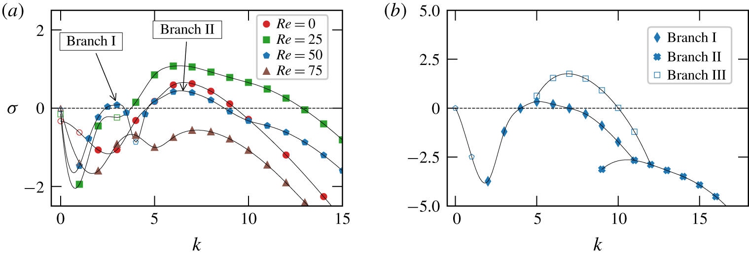
(a) Growth rates of the leading eigenmodes at  $Ra=10^{4}$ for
 $Re=0$, 25, 50, and 75. (b) Growth rates of the eigenmodes associated with branches I, II and III for
 $Re=200$ and
 $Ra=1.8\times 10^{5}$. Each curve
 $\unicode[STIX]{x1D70E}(k)$ in figure 8 corresponds to the absolute maximum growth rate over all three branches for each
 $k$.

When  $Re$ is increased from zero, the growth rate first increases for all
 $k$ (keeping the same value of
 $Ra$). Consequently, the critical Rayleigh number
 $Ra_{c}(Re)$ initially decreases up to
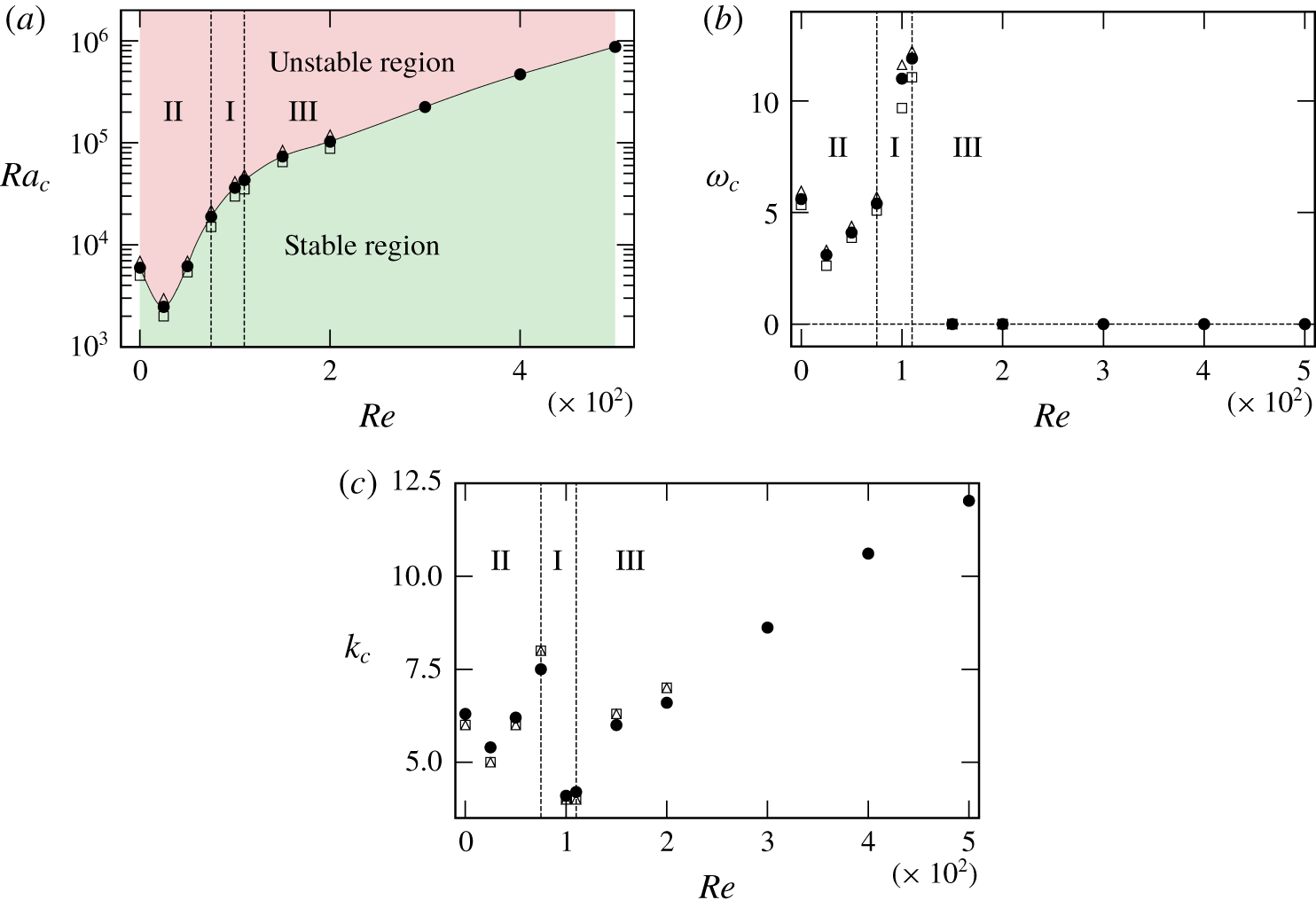
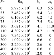
 $Re=25$ (see figure 10a and table 2). The physical reason can be traced to the structure of the two-dimensional base flow: increasing
 $Re$ from zero suppresses the secondary vortices near
 $x=0$. These give way to the main bulk cells which grow in size (see figure 6b). This implies that the effective flow length scale increases and so does the effective Rayleigh number. Consequently, a lower Rayleigh number is sufficient to trigger the instability.
For  $Re>25$, the effect is reversed. For all
 $k$,
 $\unicode[STIX]{x1D70E}(k)$ decreases, and the corresponding critical Rayleigh number
 $Ra_{c}(Re)$ increases. This time, the effect originates in the reduction in the size and intensity of the main cells in the base flow due to their suppression by the inflow near the top boundary at
 $y=1$ (see figure 6c). The decrease of
 $\unicode[STIX]{x1D70E}(k)$ is, however, not uniform over the spectrum of wavelengths and the maximum of
 $\unicode[STIX]{x1D70E}(k)$ associated with branch I increases in value compared to that associated with branch II. This effect is best illustrated in figure 9(a), which displays
 $\unicode[STIX]{x1D70E}(k)$ versus
 $k$ at a fixed value of Rayleigh number (
 $Ra=10^{4}$) for
 $Re=0$, 25, 50 and 75. From
 $Re=100$ onwards, the most unstable mode becomes associated with branch I. From this point on,
 $Ra_{c}$ continues to increase with
 $Re$ but more slowly than for
 $Re\leqslant 100$.
Up to  $Re=110$, all calculated unstable eigenmodes are oscillatory. From
 $Re=150$, a third branch (III) appears very close to branch I, with the specificity that all associated modes are non-oscillatory (i.e.
 $\unicode[STIX]{x1D714}=0$). For
 $Re\geqslant 150$, the mode associated with the maximum growth rate in branch III becomes dominant and the onset of the instability occurs through a non-oscillatory mode. The real eigenvalue associated with the single fastest growing mode is represented in the eigenvalue spectra for
 $Re=200$ and
 $Ra=1.1\times 10^{5}$ at
 $k=7$ in figure 8(f). At this point, the main cells in the base flow have disappeared. Hence, the transition from the oscillatory to the non-oscillatory instability is associated with a fundamental change in the nature of the base flow, as it switches from a recirculation-dominated topology to one dominated by the through-flow. As such, this transition separates a buoyancy-driven regime and a hydrodynamic one.
(a) Critical Rayleigh number, (b) critical frequency, and (c) critical wavenumber as a function of  $Re$. In (a) green (red) regions below (above) the curve represents flow regimes that are linearly stable (unstable) to two or three-dimensional perturbations. Symbols: ●, data obtained from the LSA; ▫, three-dimensional DNS up to
 $Re=200$ at slightly subcritical values of
 $Ra$; ▵, three-dimensional DNS up to
 $Re=200$ at slightly supercritical values of
 $Ra$.

5.2 Variations of $\unicode[STIX]{x1D714}_{c}$ and $k_{c}$ with $Re$


The variations with  $Re$ of the critical frequency
 $\unicode[STIX]{x1D714}_{c}$ and wavelength
 $k_{c}$ at the onset of instability reflect the transition between branches I, II and III, whose coexistence is illustrated in figure 9(b). As
 $Re$ increases, the variations of the frequency and wavelength associated with the maximum of each of the branches differ: for
 $Re\leqslant 100$, branch II dominates and over this interval, both
 $\unicode[STIX]{x1D714}_{c}$ and
 $k_{c}$ follow the non-monotonous variations of
 $Ra_{c}$ observed in the previous section. The switchover from branch II to branch I observed at
 $Re=100$ translates into a discontinuity in the variations of both
 $\unicode[STIX]{x1D714}_{c}$ and
 $k_{c}$. While
 $\unicode[STIX]{x1D714}_{c}$ practically doubles between
 $Re=75$ and
 $Re=100$,
 $k_{c}$ drops by half over the same interval (evaluating the exact amplitudes of these discontinuities would require a prohibitively large number of simulations). However, both
 $\unicode[STIX]{x1D714}_{c}$ and
 $k_{c}$ subsequently increase over the interval of dominance of branch I. The next discontinuity occurs at
 $Re=150$, at which point branch III becomes dominant at the expense of branch I. Since branch III modes are non-oscillatory,
 $\unicode[STIX]{x1D714}_{c}$ drops to zero. At the same time, the
 $k_{c}$ jumps up to higher values and continues to increase with
 $Re$ beyond
 $Re=150$.
Discontinuities in length scale at the onset of instabilities are frequently observed when convection is combined with forces other than buoyancy and viscosity. Usually, the discontinuity appears when a parameter representing the ratio of two of the forces in the system is varied, and it reflects the transition between different unstable modes. In rotating magnetohydrodynamic (MHD) convection, for example, a transition occurs between the thin convective plumes favoured by fast rotation and the large convective rolls, favoured by the Lorentz force. As in the present case, each of these patterns corresponds to a distinct branch of eigenmodes of the stability problem. The transition between them takes place at a critical value of the ratio between these forces. The corresponding change in length scale has been experimentally observed to reach an order of magnitude (Nakagawa Reference Nakagawa1957) in agreement with theoretical predictions (Chandrasekhar Reference Chandrasekhar1968; Aujogue, Pothérat & Sreenivasan Reference Aujogue, Pothérat and Sreenivasan2015). Similar phenomena are also observed in mixed convection in magnetic fields, at the changeover between convection dominated regimes and shear-dominated ones (Vo, Pothérat & Sheard Reference Vo, Pothérat and Sheard2017). While in rotating magnetoconvection, the transition only involves non-oscillatory modes; it only involves oscillatory ones in mixed MHD convection. The transition resembling most the one observed here, between oscillatory and non-oscillatory modes, and with a discontinuity in wavelength, was observed when decreasing the Prandtl number in rotating convection (Clune & Knobloch Reference Clune and Knobloch1993).
Finally, in the range of larger Reynolds numbers, an asymptotic behaviour associated with branch III emerges, where  $k_{c}$ scales linearly with
 $Re$ as
 $k_{c}=(3.2\pm 0.2)+(0.018\pm 0.001)Re$.
Critical Rayleigh number, corresponding wavenumber along the homogeneous direction and frequency at the onset of instability for  $Re$ ranging from zero to
 $500$.

5.3 DNS near criticality
To assess the relevance of the LSA, we perform DNS of the two-dimensional flow perturbed by white noise as described in § 3.1, for each value of  $Re$ up to 200, at slightly subcritical (
 $r_{c}<0$) and slightly supercritical (
 $r_{c}>0$) values of
 $Ra$. Here,
 $r_{c}=(Ra/Ra_{c})-1$ is the criticality parameter. The data from these DNS, including
 $Ra$, measured frequency and wavelength, are represented in figure 10. We stress that the primary purpose here is not one of validation of the growth rate obtained by LSA (even though this comes as a by-product), but to answer the question of whether the LSA correctly identifies the mode that ‘naturally’ emerges from an unstable base state. As such, it is essential that the initial condition be unbiased towards a particular mode. This is the reason why white noise, rather than the most unstable mode, is used to perturb the base state in the initial condition.
In all investigated cases, the perturbation was found to decay for  $Ra<Ra_{c}$ and the flow to bifurcate away from the base state for
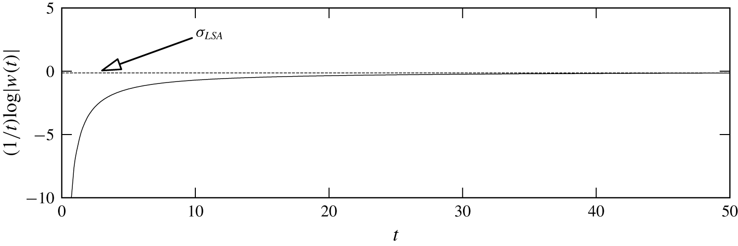
 $Ra>Ra_{c}$. The subcritical decay rate was extracted from the DNS with an exponential fit to the long-time decay of
 $w$ measured at a single point in the domain as shown in figure 11 for
 $Re=200$ and
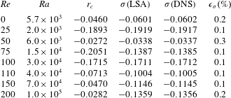
 $Ra=10^{5}$. The asymptotic decay rate was always found within 0.3 % of the prediction of the LSA, confirming that the fully nonlinear decay is dominated by the leading mode returned by the linear stability (see table 3 for details).
Further confirmation that the leading mode identified by LSA drives the dynamics near  $Ra=Ra_{c}$ is found by comparing critical frequencies and wavelengths,
 $\unicode[STIX]{x1D714}_{c}$,
 $k_{c}$. In the DNS, the perturbation is isolated by subtracting the steady two-dimensional base solution from the result of the time-dependent three-dimensional simulation. Again, an agreement with a relative error lower than 2 % is found between the DNS and the LSA.
Decay rate built on the time history of the  $w(t)$ velocity component at
 $(x,y,z)=(0,0.6,0.5)$ obtained by DNS for
 $Re=200$ and
 $Ra=10^{5}$, compared to the growth rate obtained by LSA.

Comparison of the decay rate computed from the LSA and DNS for  $r_{c}<0$. The relative error in the computation of growth rate from DNS and LSA is represented by
 $\unicode[STIX]{x1D716}_{\unicode[STIX]{x1D70E}}$.

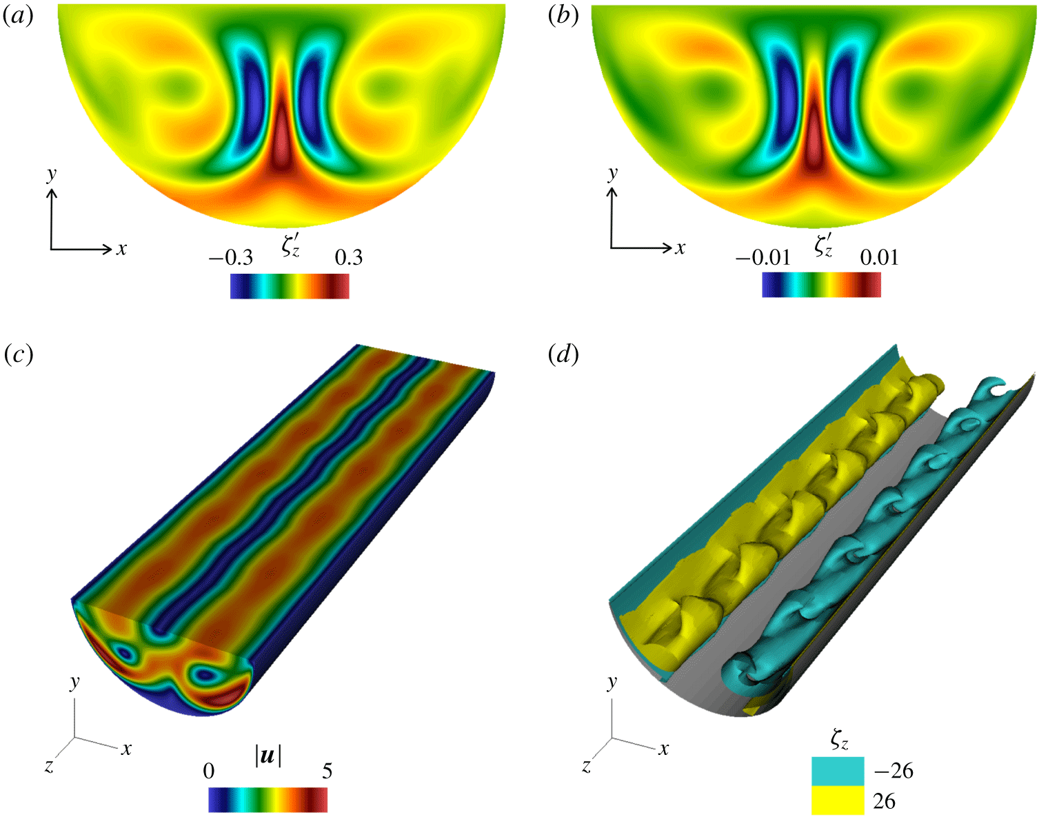
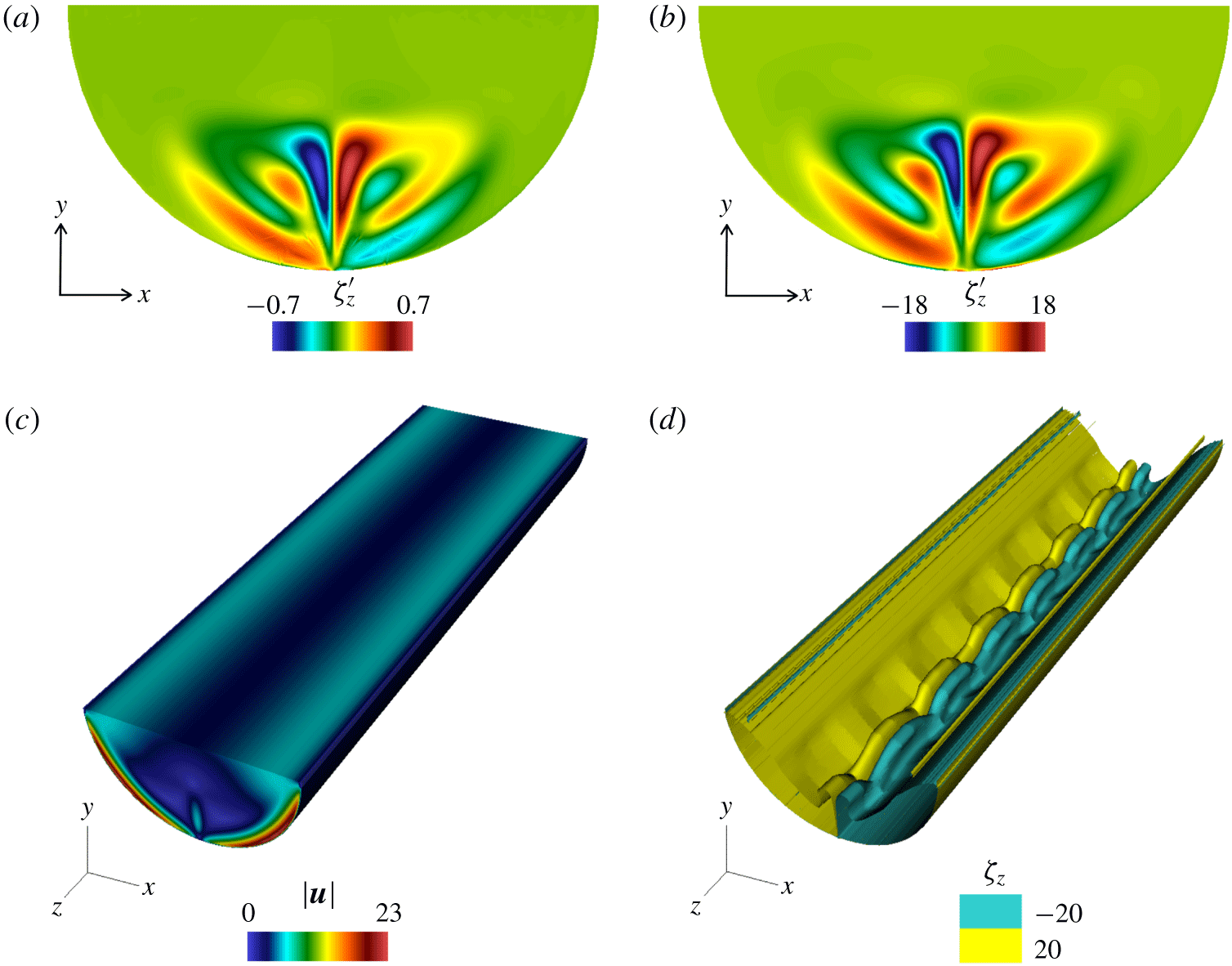
For  $Re=0$ and
 $Ra=7\times 10^{3}$: (a) vorticity perturbation along the homogeneous direction
 $\unicode[STIX]{x1D701}_{z}^{\prime }$ computed from the LSA at
 $z=0$ plane for
 $k=6$; (b) vorticity perturbation along the homogeneous direction
 $\unicode[STIX]{x1D701}_{z}^{\prime }$ computed from the DNS at
 $z=0$ plane; (c) density plot for the magnitude of the velocity field and (d) iso-surfaces of the
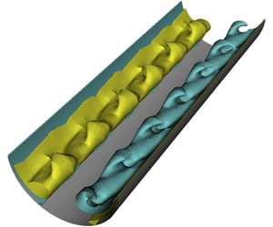
 $z$-component of vorticity. A movie representing the travelling wave is available in the supplementary material (see supplementary movie 1, available at https://doi.org/10.1017/jfm.2019.1015).

5.4 Topology and time-dependence of the perturbation near criticality
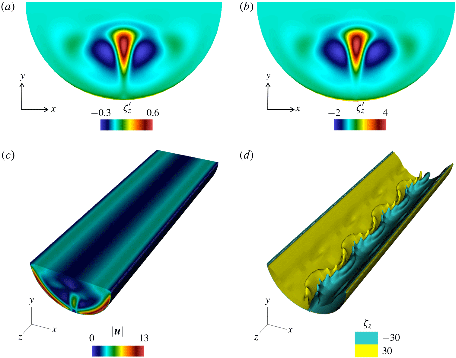
Figures 12, 13 and 14, respectively, show the velocity magnitudes and vorticity distributions in weakly supercritical cases associated with each of the three instability branches (respectively, for  $Re=0$,
 $Re=100$ and
 $Re=200$). The time evolution of the perturbation reconstructed from the LSA involves both real and imaginary parts as of the LSA eigenvector
 $$\begin{eqnarray}\boldsymbol{q}^{\prime }(x,y,z,t)=Re\{\hat{\boldsymbol{q}}(x,y)\text{e}^{\unicode[STIX]{x1D70E}t+\text{i}(kz+\unicode[STIX]{x1D714}t)}\}.\end{eqnarray}$$
The snapshots of the topologies of the perturbation from LSA and DNS presented on the figures are captured at the same phase.
Unsurprisingly, the topologies of the perturbations found in the DNS and LSA precisely agree too. In all cases, the instability originates near the symmetry plane  $x=0$, just above the location where the jets driven by the baroclinic imbalance on either side of the cavity meet. The driving mechanism is a destabilisation of the return jet, with a different behaviour depending on the branch the unstable mode belongs to: modes from branch II (
 $Re<75$) develop into a travelling wave along
 $\boldsymbol{e}_{z}$. Since the travelling wave is made up of two counter-propagative linear waves (respectively, associated with each of the conjugate eigenvalues), the travelling nature of the wave is determined by the complex amplitude of the unstable modes (Clune & Knobloch Reference Clune and Knobloch1993). These cannot be obtained from LSA but appear in the fully nonlinear DNS (see figure 12 and associated animation). By contrast, modes from branch I, which are the most unstable for
 $100\leqslant Re\leqslant 110$, always develop into a standing wave with transverse oscillations within the
 $x\text{-}y$ plane.
For  $Re=100$ and
 $Ra=4\times 10^{4}$: (a) vorticity perturbation along the homogeneous direction
 $\unicode[STIX]{x1D701}_{z}^{\prime }$ computed from the LSA at
 $z=0$ plane for
 $k=4$; (b) vorticity perturbation along the homogeneous direction
 $\unicode[STIX]{x1D701}_{z}^{\prime }$ computed from the DNS at
 $z=0$ plane; (c) density plot for the magnitude of the velocity field and (d) iso-surfaces of the
 $z$-component of vorticity. A movie representing the standing wave is available in the supplementary material (see supplementary movie 2).

For  $Re=200$ and
 $Ra=1.1\times 10^{5}$: (a) vorticity perturbation along the homogeneous direction
 $\unicode[STIX]{x1D701}_{z}^{\prime }$ computed from the LSA at
 $z=0$ plane for
 $k=7$; (b) vorticity perturbation along the homogeneous direction
 $\unicode[STIX]{x1D701}_{z}^{\prime }$ computed from the DNS at
 $z=0$ plane; (c) density plot for the magnitude of the velocity field and (d) iso-surfaces of the
 $z$-component of vorticity.

6 Characterisation of the transition to oscillatory and non-oscillatory states
6.1 Stuart–Landau model
We now seek to characterise the bifurcation associated with the instabilities identified in the previous section by means of a truncated Stuart–Landau equation. This model has been widely applied to find the nature of bifurcations in a number of fluid flows, for example, flow past a circular cylinder (Provansal, Mathis & Boyer Reference Provansal, Mathis and Boyer1987; Dušek, Le Gal & Fraunié Reference Dušek, Le Gal and Fraunié1994; Schumm, Berger & Monkewitz Reference Schumm, Berger and Monkewitz1994; Albarède & Provansal Reference Albarède and Provansal1995; Henderson & Barkley Reference Henderson and Barkley1996; Thompson & Le Gal Reference Thompson and Le Gal2004), staggered cylinder (Carmo et al. Reference Carmo, Sherwin, Bearman and Willden2008) and rings (Sheard et al. Reference Sheard, Thompson and Hourigan2004), and the flow confined around a  $180^{\circ }$ sharp bend (Sapardi et al. Reference Sapardi, Hussam, Pothérat and Sheard2017; Pothérat & Zhang Reference Pothérat and Zhang2018). The principle traces back to the equation proposed by Landau (Reference Landau1944) to describe the transition to turbulence, and later used by Stuart (Reference Stuart1958, Reference Stuart1960) to understand the behaviour of the plane Poiseuille flow. The Stuart–Landau model describes the growth and saturation of the complex amplitude
 $A(t)$ of a perturbation near the onset of instability as (Landau & Lifsitz Reference Landau and Lifsitz1987)
 $$\begin{eqnarray}\frac{\text{d}A}{\text{d}t}=(\unicode[STIX]{x1D70E}+\text{i}\unicode[STIX]{x1D714})A-l(1+\text{i}c)|A|^{2}A+O(A^{5}),\end{eqnarray}$$
where  $l\in \mathbb{R}$ reflects the level of nonlinear saturation and
 $c\in \mathbb{R}$ is the Landau constant. For
 $l>0$, the first two terms on the right-hand side of (6.1) provide a good description of the evolution of the perturbation, and the saturation occurs through the cubic term. In this case, the bifurcation is supercritical. For
 $l<0$, the cubic term accelerates the growth of the perturbation, and higher-order terms are needed to saturate the growth. This case corresponds to a subcritical transition. The equations for the time evolution of the (real) amplitude
 $|A(t)|$ and phase
 $\unicode[STIX]{x1D719}(t)$ are obtained by substituting
 $A(t)=|A(t)|\text{e}^{\text{i}\unicode[STIX]{x1D719}(t)}$ into (6.1) and separating the real and imaginary parts:
 $$\begin{eqnarray}\displaystyle & \displaystyle \frac{\text{d}|A|}{\text{d}t}=\unicode[STIX]{x1D70E}|A|-l|A|^{3}, & \displaystyle\end{eqnarray}$$
 $$\begin{eqnarray}\displaystyle & \displaystyle \frac{\text{d}\unicode[STIX]{x1D719}}{\text{d}t}=\unicode[STIX]{x1D714}-lc|A|^{2}. & \displaystyle\end{eqnarray}$$
Equation (6.2) is rewritten as
 $$\begin{eqnarray}\frac{\text{d}\log |A|}{\text{d}t}=\unicode[STIX]{x1D70E}-l|A|^{2}.\end{eqnarray}$$
As noted by Sheard et al. (Reference Sheard, Thompson and Hourigan2004), this form of the Stuart–Landau equation makes it convenient to determine  $\unicode[STIX]{x1D70E}$ and
 $l$ from three-dimensional DNS (see § 6.2) if
 $A(t)$ is defined as the time-dependent amplitude of one component of the velocity perturbation, for example. The amplitude of the perturbation in the saturated state is readily obtained by setting
 $\unicode[STIX]{x2202}_{t}=0$ in (6.2):
 $$\begin{eqnarray}|A_{sat}|=\sqrt{\frac{\unicode[STIX]{x1D70E}}{l}}.\end{eqnarray}$$
Furthermore, if the flow settles down to a time-periodic state with constant amplitude  $|A_{sat}|$,
 $\text{d}\unicode[STIX]{x1D719}/\text{d}t$ becomes the constant angular frequency of oscillation
 $\unicode[STIX]{x1D714}_{sat}$, and (6.3) yields
 $$\begin{eqnarray}c=\frac{\unicode[STIX]{x1D714}_{sat}-\unicode[STIX]{x1D714}}{\unicode[STIX]{x1D70E}}.\end{eqnarray}$$
Thus, the Landau constant  $c$ can be determined by computing the oscillation frequency of the perturbation in the linear regime and at the saturation.
6.2 Nature of the bifurcations
We shall first determine the nature of the bifurcation by calculating constant  $l$ and checking its sign. We follow Sheard et al. (Reference Sheard, Thompson and Hourigan2004) and fit equation (6.4) to the time variation of the envelope of
 $|A(t)|$ extracted from the signal of the
 $z$-component of velocity
 $w(t)$ obtained at a single location, in the neighbourhood of
 $|A|=0$. This particular choice for
 $|A(t)|$ and the choice of location itself are guided by the requirement of obtaining a clean enough signal. Other choices are possible (Sheard et al. Reference Sheard, Thompson and Hourigan2004), based on either local or global variables (Pothérat & Zhang Reference Pothérat and Zhang2018). The analysis has been carried out in slightly supercritical regimes (
 $r_{c}>0$, but small) for all values of
 $Re$ investigated in this paper up to
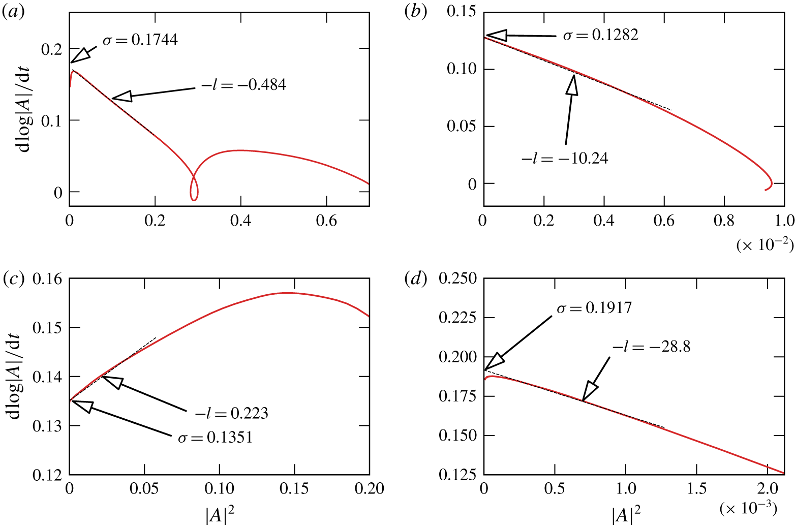
 $200$. Four representative examples are shown on figure 15. In all cases, a small area very close to
 $|A|=0$ is dominated by numerical noise. The high precision of our DNS, however, keeps this interval small compared to the area where the linear approximation (6.4) remains valid. Fitting of (6.4) in the linear range provides the values of
 $\unicode[STIX]{x1D70E}$ and
 $l$. Comparing
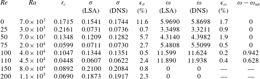
 $\unicode[STIX]{x1D70E}$ to the value returned by the LSA provides not only mutual validation for the linear stability and the DNS, but also an estimate for the precision of the fit. Both values are reported in table 4. The relative discrepancy remains below 6 % except for
 $Re=0$, where the discrepancy is of 11.6 %.
Stuart–Landau analysis: variation of  $(\text{d}\text{log}|A|/\text{d}t)$ versus
 $|A|^{2}$ and extrapolation to
 $|A|=0$ from which coefficients
 $\unicode[STIX]{x1D70E}$ and
 $l$ are obtained for (a)
 $Re=0$,
 $Ra=7\times 10^{3}$; (b)
 $Re=50$,
 $Ra=7\times 10^{3}$; (c)
 $Re=100$,
 $Ra=4\times 10^{4}$; and (d)
 $Re=200$,
 $Ra=1.1\times 10^{5}$. Here,
 $|A(t)|$ is obtained from time-series of
 $w(t)$.

Comparison of the growth rate and frequency computed from the LSA and DNS for  $r_{c}>0$. The relative error in the computation of frequency from DNS and LSA is represented by
 $\unicode[STIX]{x1D716}_{\unicode[STIX]{x1D714}}$.

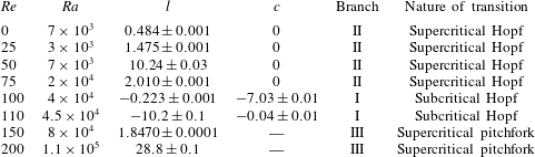
At the onset of instability,  $l$ remains positive for
 $0\geqslant Re\geqslant 75$, which corresponds to the range of values of
 $Re$ where the instability sets in through branch II modes. In other words, branch II modes become unstable through a supercritical Hopf bifurcation. For
 $100\leqslant Re<150$, by contrast,
 $l<0$ indicates that the modes of branch I destabilise through a subcritical Hopf bifurcation. This may appear as surprising considering the very good agreement between the critical Rayleigh number for the onset of instability found by DNS and LSA. Nevertheless, the small value of
 $l$ suggests that the system may only be mildly subcritical. It is also possible that the addition of white noise of moderate amplitude may not suffice to drive the growth of subcritical perturbations. Indeed, we verified that further increasing the standard deviation of the added white noise to 0.01 and 0.1 did not alter the results. Whether transition could occur for
 $Ra<Ra_{c}$ could be answered by analysing whether non-modal perturbations could grow (Schmid & Henningson Reference Schmid and Henningson2001), and whether optimal perturbation of sufficient amplitudes could trigger a subcritical transition to another state, as it does for turbulence in pipes (Pringle, Willis & Kerswell Reference Pringle, Willis and Kerswell2012). For
 $Re\geqslant 150$, the instability occurs through non-oscillatory modes from branch III;
 $l$ becomes positive again, indicating that this transition is of supercritical type (supercritical pitchfork). In contrast with bifurcation through branch I, the supercritical nature of the instability of modes from branches II and III is consistent with the excellent agreement between LSA and DNS on the value of
 $Ra$ for the onset of instability and further establishes the relevance of LSA to determine the stability of the flow in these cases.
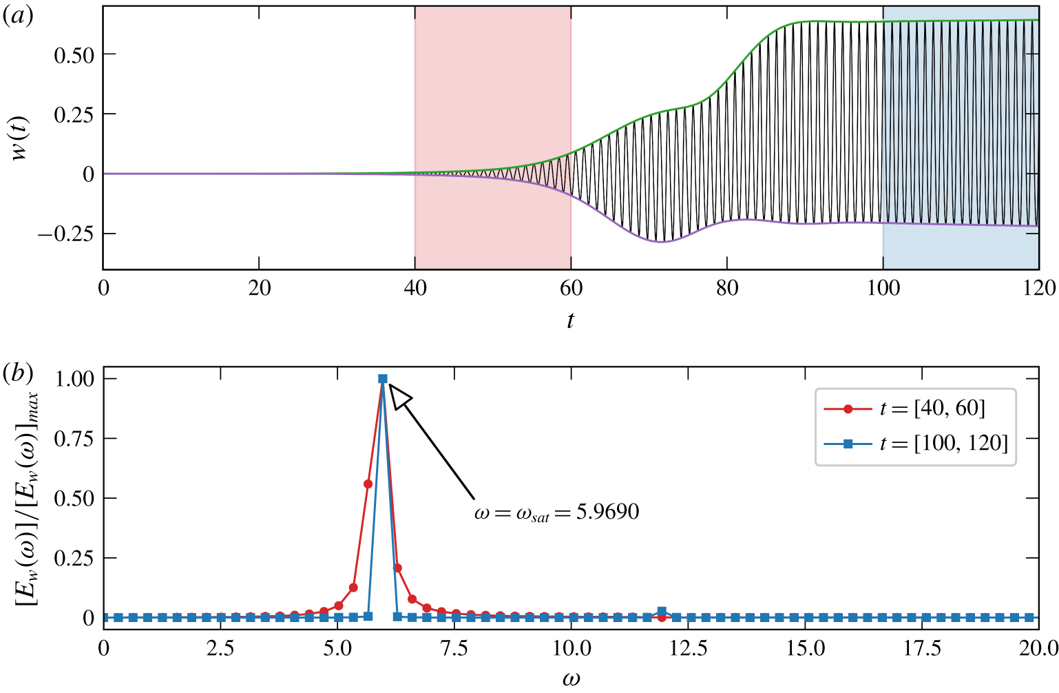
(a) Time history of  $w(t)$ velocity component measured at
 $(x,y,z)=(-0.6,0.6,0.5)$ for
 $Re=0$ and
 $Ra=7\times 10^{3}$. (b) Frequency spectra obtained from the time series of
 $w(t)$, respectively, near the onset and near saturation.

6.3 Saturated states
Finally, we shall characterise the saturated states. The analysis was carried out for each investigated value of  $Re$ up to
 $Re=200$, of which we present three typical cases. As discussed in § 5.3, the three-dimensional DNS were performed for two values of
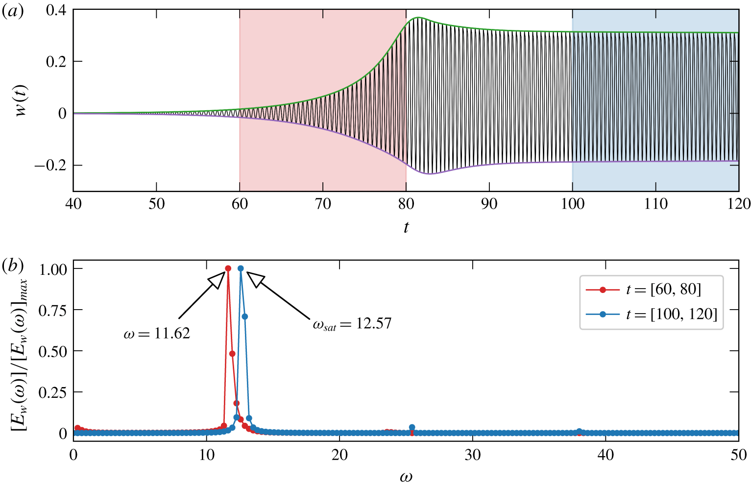
 $Ra$ in each case, one slightly subcritical and one slightly supercritical. As an example, figure 16(a) shows the time history of
 $w$ at a single point of the domain for the weakly supercritical case of
 $Re=0$ and
 $Ra=7\times 10^{3}$. The normalised frequency spectrum of the time-series
 $$\begin{eqnarray}E_{w}(\unicode[STIX]{x1D714})={\textstyle \frac{1}{2}}|{\hat{w}}(\unicode[STIX]{x1D714})|^{2},\end{eqnarray}$$
where  ${\hat{w}}(\unicode[STIX]{x1D714})$ is the Fourier transform of
 $w(t)$, is then calculated over two intervals: one near the onset (
 $40\leqslant t\leqslant 60$) and one in the saturated regime (
 $100\leqslant t\leqslant 120$). Both are represented in figure 16(b). The initial and saturated frequencies are nearly identical (with relative error to the numerical precision) and differ by 1.7 % from the frequency returned by the LSA. Given that the discrepancy between the frequencies near the onset and in the saturated state differ by much less than the error between the frequency near the onset predicted by LSA and DNS, we consider them to be identical. In this case, from equation (6.6), the Landau constant
 $c$ is zero, to the precision of our simulations. Following this approach, non-zero values of
 $c$ were found for other values of
 $Re$ when
 $\unicode[STIX]{x1D714}-\unicode[STIX]{x1D714}_{sat}$ significantly exceeded the discrepancy between LSA and DNS. One such example is shown in figure 17, for
 $Re=100$, where
 $c=-7.03\pm 0.01$ and the discrepancy between LSA and DNS frequencies at onset is 0.2 %.
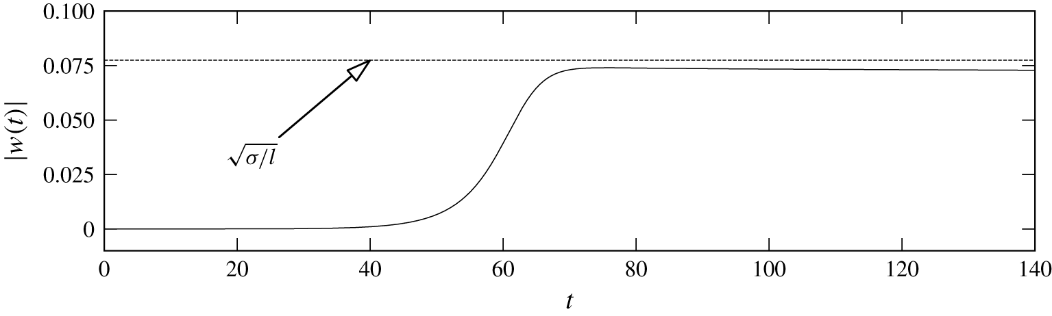
All calculated values of  $c$ are reported in table 5. Here again, the three branches identified in § 5 exhibit different behaviours: when the instability arises out of modes in branch II, the Landau constant is zero. A shift in frequency does appear as soon as the instability is due to modes belonging to branch I, leading to a negative Landau constant. Finally, as branch III becomes dominant, DNS confirm that the steady saturated state of the mode predicted by the linear stability is non-oscillatory. In this case, the saturated amplitude predicted by (6.5) matches closely that observed in the DNS, as shown on figure 18.
(a) Time history of  $w(t)$ velocity component measured at
 $(x,y,z)=(-0.6,0.6,0.5)$ for
 $Re=100$ and
 $Ra=4\times 10^{4}$. (b) Frequency spectra obtained from the time series of
 $w(t)$, respectively, near the onset and near saturation.

6.4 Heat flux in the saturated states
To finish, we compare the Nusselt number  $Nu$ in base two-dimensional state and the bifurcated three-dimensional state at the onset of instability for all Reynolds numbers in figure 7(b). The maximum difference between them is 0.2 %. Thus, there is hardly any change in the heat transfer. This can be understood as the boundary conditions impose that the horizontal heat flux must be conserved between the two boundaries with periodic boundary conditions. This precludes any horizontal redirection of the horizontal heat flux. Furthermore, the time and spatially periodic character of the instability implies that a drastic change would have had to take place between the streamlines in the
 $(x\text{-}y)$ plane of the base flow and those of the bifurcated states for a significant change in
 $Nu$ to be observed. Nevertheless, figure 7(b) expresses that heat transfer at the onset of the instability decreases with
 $Re$ because of the suppression of the convection by the through-flow.
Time history of  $w(t)$ velocity component measured at
 $(x,y,z)=(-0.5,0.6,0.5)$ for
 $Re=200$ and
 $Ra=1.1\times 10^{5}$.

Summary of Stuart–Landau analysis of three-dimensional DNS for  $Re=0$ to
 $Re=200$ at
 $Ra>Ra_{c}$.

7 Conclusions
We presented a systematic analysis of the mixed baroclinic convection in a pool with hot homogeneous through-flow fed in at the upper boundary and escaping through a porous, semicircular, cold isothermal lower boundary. Linear stability analysis, DNS and bifurcation analysis have brought answers to the four questions set out in the introduction:
(i) The base flow is driven by a baroclinic imbalance along the lower boundary that peaks at its corners. Downward flows on either side of the pool meet in the symmetry plane to form two two-dimensional counter-rotating rolls. Being deprived of shear, the sole effect of the through-flow on the base flow is to displace the convective rolls downward. Once these are confined by the lower boundary, further increasing the through-flow (i.e.
$Re$) leads to their progressive suppression and their eventual disappearance for $Re\geqslant 200$. Interestingly, at low through-flow, this type of convection is less effective at carrying the heat downward as conduction in solid moving downwards at the same velocity.(ii) A consequence of the suppression of the rolls is the stabilisation of the flow to infinitesimal disturbances. Indeed, the critical Rayleigh number for linear stability of the base flow
$Ra_{c}$ first decreases as the rolls are stretched down ($Re\leqslant 25$), then increases with $Re$ as they become suppressed.(iii) The base flow was found susceptible to three distinct types of infinitesimal perturbations, all of them with maximum vorticity near the symmetry plane, where the rolls meet. For
$Re\leqslant 75$, the most unstable mode (type II) is a wave travelling in the $\boldsymbol{e}_{z}$ direction. For $100\leqslant Re\leqslant 110$, instability sets in as a standing oscillation (type I mode), whereas for $Re\geqslant 150$ the dominating mode is non-oscillating (type III). The DNS have confirmed the findings of the LSA, both in terms of topology of the modes and the critical parameters at the onset (critical Rayleigh number, wavelength and frequencies).(iv) Most interestingly, Stuart–Landau analysis conducted on DNS data revealed that the nature of the bifurcation associated with the three modes varies too. While mode II and III appear at a supercritical bifurcation, the onset of mode I is subcritical.


Nevertheless, the values of the constant  $l$ indicate a low level of subcriticality. This may partly explain why LSA and DNS are still in agreement at the onset of the subcritical branch. Still, the change of nature of the bifurcation near the onset is an interesting feature of this problem. It raises the question of whether the system would support other convective states located on subcritical branches not connected to the base state considered in this study. These would need to be ignited from a different set of initial conditions. Such phenomenology was recently found in numerical models for rotating convection in the Earth’s core, where the curvature of the boundaries plays an important role too (Guervilly & Cardin Reference Guervilly and Cardin2016).
These results introduce a number of new features, compared to the reference cases of convection in an inclined channel (Gage & Reid Reference Gage and Reid1968) and mixed convection in a cavity (Papanicolaou & Jaluria Reference Papanicolaou and Jaluria1992), despite the similarities pointed out in introduction. Unlike convection in an inclined channel, longitudinal rolls are present in the base flow because the close, semicircular shape of the boundary does not support an open flow in the direction of the baroclinic jets. As such, all unstable modes involve a form of longitudinal variation. As direct consequence, the transversal travelling waves found in inclined channels cannot exist, but, remarkably, longitudinal travelling waves exist instead. Furthermore, while travelling waves found in the inclined channel problem are always subject to a secondary instability, they evolve into a stable periodic flow in our semicylindrical geometry. Unlike the cavity flow where the through-flow is located on one side (Papanicolaou & Jaluria Reference Papanicolaou and Jaluria1992), the homogeneous through-flow studied here suppresses wave propagation, which turns into standing oscillations for  $Re\geqslant 100$ and finally into a non-oscillatory unstable mode for
 $Re\geqslant 150$.
Finally, the relevance of these findings to continuous casting is again partial: we do not submit the phenomenology found here as a full explanation of the dynamics of these processes. Nevertheless, evidence of oscillatory phenomena in continuous casting processes (Dorward, Beerntsen & Brwon Reference Dorward, Beerntsen and Brwon1996) suggests that the physical mechanisms involved play a role among other effects. The phenomena we described may be observed in some form, in specific configurations where they are not overshadowed by other mechanisms not considered here (such as double diffusion or variations of the pool shape with the flow parameters).
Acknowledgements
This research was funded by Constellium Technology Center (C-TEC). We thank H. M. Blackburn and D. Moxey for helping in adapting the codes DOG and Nektar++, respectively. A. Pothérat acknowledges support from the Royal Society under the Wolfson Research Merit Award Scheme (grant reference WM140032).
Declaration of interests
The authors report no conflict of interest.
Supplementary movies
Supplementary movies are available at https://doi.org/10.1017/jfm.2019.1015.