Introduction
The increasing demand for more advanced communication systems with wider channel bandwidths has recently motivated space companies to explore the use of higher frequency bands (such as Ku, K, and Ka) that can easily accommodate higher transmission rates [1].
However, the use of higher frequency bands poses a series of mechanical problems when manufacturing waveguide devices in general, and in particular with respect to waveguide filters. It is, in fact, well known that as the frequency increases, the wavelength decreases, and the physical size of the components becomes smaller. As a result, the devices become much more sensitive to errors in the manufacturing processes. A practical solution to compensate for the errors without greatly increasing the cost of the filters is to use a manufacturing technique with an intermediate accuracy, like milling, and to use tuning elements to recover the desired response.
This, in turn, introduces a complication, namely, the manual tuning of the filter after manufacturing. Adjusting manually the tuning elements of a filter is, in fact, a complex and time-consuming task that, in general, requires extensive tuning experience [Reference Snyder2].
Furthermore, the use of milling and tuning elements introduces two more challenges. The first one is that using milling we inevitably introduce rounded corners in the hardware. The rounded corners must then be included in the electromagnetic (EM) simulations, and this can significantly increase the required computational effort. The second challenge is that the presence of tuning elements must also be taken into account, and this can increase even further the computational effort. In this context, we must also remember that most microwave filter structures are currently designed using optimization procedures that normally require a large number of repeated EM simulations. A small increase in the time required for the EM simulation can therefore have a very significant negative effect.
Fortunately, however, the field of EM-based optimization of complex structures has recently made very significant progress due to the introduction of Space Mapping (SM) [Reference Bandler, Biernacki, Chen, Grobelny and Hemmers3] and Aggressive Space Mapping (ASM) [Reference Bandler, Biernacki, Chen, Hemmers and Madsen4–Reference Koziel15]. SM uses two simulation spaces, or models. A fast and low accuracy model, the so-called coarse model, and a precise but time-consuming model, the so-called fine model. The basic idea behind SM (and ASM) is that most simulations are performed using the coarse model, and the fine model is only used to verify the performance of the device in the various stages of the optimization process.
Significant effort has also been devoted in the past to the development of advanced CAD filter tuning procedures. Examples are the use of fuzzy logic [Reference Miraftab and Mansour16], and machine learning [Reference Mirzai, Cowan and Crawford17, Reference Zhou and Huang18], to cite a few. A significant recent development in this area has been the use of SM to develop very efficient and effective CAD tuning procedures [Reference Melgarejo, Guglielmi, Cogollos and Boria19, Reference Melgarejo, Ossorio, Cogollos, Guglielmi, Boria and Bandler20].
In this context, therefore, the objective of this contribution is to provide, in a single paper, detailed information about the use of advanced SM techniques for both filter design and tuning. In addition to theory, we discuss in detail the design and tuning process of two types of filters that are commonly used for both ground and for space applications, namely, an inductive rectangular waveguide filter, and a more complex dual-mode filter.
The remainder of the paper is organized as follows. In Section “Design techniques”, we discuss in detail the design of the filters. In Section “Tuning techniques”, we show the most adequate tuning strategy to be used in each case. Finally, in Section “Conclusions”, we conclude the paper with a summary of the results that we have obtained.
Design techniques
In this section, we show how to design an inductive filter in rectangular waveguide and a compact filter based on dual-mode resonators. For each case, we compare the performances of two ASM-based design procedures [Reference Ossorio, Melgarejo, Boria, Guglielmi and Bandler11, Reference Melgarejo, Guglielmi, Cogollos and Boria12].
Inductive filter
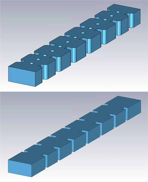
Inductive filters in rectangular waveguide are very commonly used for both ground and space applications. In this section, we describe the design procedure for the six-pole filter shown in Fig. 1 (top). The center frequency of the filter is 11 GHz, and the bandwidth is 500 MHz. In order to reduce production costs, the filter will be manufactured using H-plane milling with an intermediate accuracy, namely, between 50 and 100 μm. As a consequence, all concave corners will be rounded in the final hardware. The filter will also use tuning elements (with 1.6 mm radius) both in the cavities and in the coupling irises. In the design process, all the tuners will be set to a penetration of 2 mm. This value is chosen to allow for future bidirectional adjustments.
Inductive six-pole filter. Top: Fine model of the filter. Bottom: Ideal coarse model of the filter.

The design process starts with a distributed model based on transmission lines and inverters that produce the desired Chebyshev response, i.e. the target of our design. Once we have obtained the distributed model, we can apply the design procedure described in [Reference Guglielmi and Melcon21] in order to obtain the initial ideal waveguide model of the filter shown in Fig. 1 (bottom). If we use a Multimode Equivalent Network (MEN) simulator, such as FEST3D, with a low accuracy setting, the EM analysis will require a very short time, and we will be able to rapidly optimize the structure and obtain the desired target performance.
At this point, the most time-consuming part of the design begins: we need to include all non-ideal elements, namely, the tuning elements and the rounded corners, and optimize the final filter structure with a high accuracy simulator. We could decide, for instance, to use FEST3D in a high accuracy setting, or a finite-element method solver, like CST or HFSS. In any case, the time required to carry out this step will be significant. We will now show how ASM can be very effectively exploited to reduce very significantly the computational effort.
OS-ASM
As already mentioned, the idea behind any SM-based optimization method is to use two simulations models: a fast model, called the coarse model (or space), and a precise but time-consuming model, the fine model. The key assumption behind SM (and ASM) is that the two spaces are related by the following linear equation (or mapping):

where xf and xc are the dimensions of the fine (Fig. 1, top) and coarse (Fig. 1, bottom) models, respectively. Furthermore, if we call the performances in the two spaces R f(xf) and R c(xc), respectively, we can write:

to state that we have the same identical response in the two spaces. This is, in fact the objective that we want to obtain, namely, a set of dimensions for a filter structure that when manufactured and measured gives the same exact response of our ideal filter.
The matrix B in (1) is the so-called mapping matrix between the two spaces, and C is a vector of constants. In the traditional ASM optimization procedure [Reference Bandler, Biernacki, Chen, Hemmers and Madsen4], B is first set to be equal to the identity matrix, and it is then updated after each iteration. At the end of the process, when we reach the condition stated in (2), we can say that the coarse and fine models are perfectly aligned, and the matrix B correctly maps both spaces. Furthermore, it can be demonstrated mathematically that this optimization process will converge in a number of iterations that is proportional to the number of variables involved in the process.
Furthermore, recent research on ASM [Reference Ossorio, Melgarejo, Boria, Guglielmi and Bandler11] indicates that the matrix B has the following, very important property. If the geometry of the coarse model is exactly identical to the geometry of the fine model, and the only difference between the two spaces is the accuracy of the computations, the correct value of B is, in fact, the identity matrix, and the ASM optimization process converges in just one step. This is, indeed, the origin for the name One-Step ASM (OS-ASM) in [Reference Ossorio, Melgarejo, Boria, Guglielmi and Bandler11].
In the case we are discussing now, however, the coarse and the fine models are not exactly identical, as we can see in Fig. 1. The OS-ASM optimization process will therefore not be able to converge in one single step. However, the results obtained in [Reference Ossorio, Melgarejo, Boria, Guglielmi and Bandler11] indicate that, using the identity matrix as the mapping matrix will result in a faster convergence with respect to the original ASM procedure described in [Reference Bandler, Biernacki, Chen, Hemmers and Madsen4].
The OS-ASM design process of the six-pole filter under examination is detailed next.
(i) Obtain first the (optimum) dimensions of the coarse model of the filter using, for instance, the procedure described in [Reference Guglielmi and Melcon21].
(ii) Set the initial dimensions of the fine model to the optimum dimensions of the coarse model (i.e. xf1 = xcopt), and add all non-ideal elements. Next carry out the first high accuracy simulation. Naturally, the electrical response that we obtain (R f(xf1)) will be (strongly) detuned (R f(xf1) ≠ R c(xcopt)).
(iii) Optimize one instance of the coarse model until the performance of the fine model is matched, that is R c(xc1) = R f(xf1).
(iv) The next step is to compute the following differences:
(3)$$\Delta = {\bf x}_{{\bf copt}}- {\bf x}_{{\bf c1}}$$
(v) We then update the dimensions of the fine model using the following equation:
(4)$${\bf x}_{{\bf f2}} = {\bf x}_{{\bf f1}} - \Delta$$and perform another fine model simulation.(vi) At this point we have completed the first iteration. We can therefore evaluate the error between R f(xf2) and the desired target response. If the error is acceptable, we have concluded our process. If it is not acceptable, we go back to the second step and perform another iteration using xf2 as a starting point.


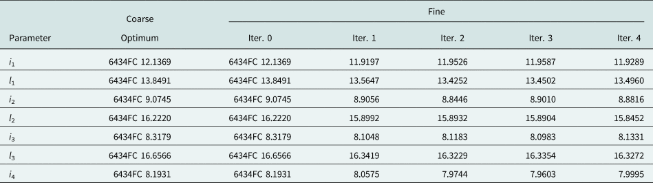
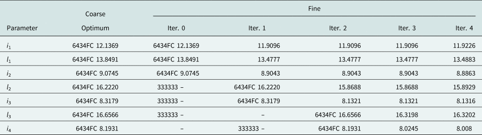
Applying to our filter the procedure just described, the coarse and fine models give essentially the same response after only four iterations. Table 1 shows the evolution of the design parameters in the OS-ASM process.
Evolution of the design parameters for the inductive six-pole filter in the OS-ASM process. The design variables are the widths of the apertures (their thickness is fixed to 3.5 mm) and the lengths of the resonators (their heights and widths are set to 9.525 and 19.95 mm). All dimensions are in mm

Efficient ASM
A more efficient alternative is to use the approach described in [Reference Melgarejo, Guglielmi, Cogollos and Boria12]. This second method combines the segmentation strategy of [Reference Guglielmi and Melcon21] with the power of OS-ASM. Instead of trying to optimize all design parameters simultaneously, the filter is designed step by step as follows:
(i) Obtain first the (optimum) dimensions of the low accuracy model of the filter.
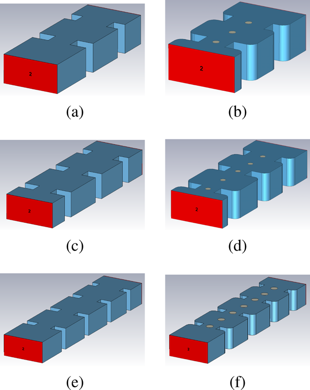
(ii) Simulate the first three elements of the low accuracy model, namely, the first cavity with the relative input and output irises (see Fig. 2(a)). This model provides the first target that the equivalent high accuracy model of the filter (see Fig. 2(b)) must match.
(iii) Perform an OS-ASM iteration with the reduced coarse and fine models (shown in Figs 2(a) and 2(b)) until the reduced fine model produces the desired target response. Note that since we are dealing with reduced models, there are only three parameters to optimize, namely, the widths of the first two apertures and the length of the first cavity.
(iv) Add the next cavity of the filter to the reduced coarse model and obtain the second target. Add that same cavity to the fine model (including rounded corners and all tuners, as shown in Fig. 2(d)). We now perform another set of ASM iterations with the reduced coarse model shown in Fig. 2(c). It is important to note that, since the first three elements of the filter have already been obtained, we only need to optimize the newly added parameters (the length of the second cavity, and the width of the output aperture). For some filters, a final optimization of all five parameters may be required to obtain a very good final agreement with the target response, however, this is not the case for our inductive filter.
(v) This procedure is repeated until we reach the center of the filter (see Fig. 2(f)).
(vi) We now have obtained a very good starting point for all the dimensions of our filter since the structure is symmetric (Fig. 1 top). At this point, we will perform a final OS-ASM optimization using all design parameters to obtain the desired final performance. This step is normally very fast, since the response of the filter is already very close to the target performance.
Filter models used in the first stage of the Efficient ASM: (a) coarse model; (b) fine model. Filter models used in the second stage: (c) coarse model; (d) fine model. Filter models used in the third stage: (e) coarse model; (f) fine model.

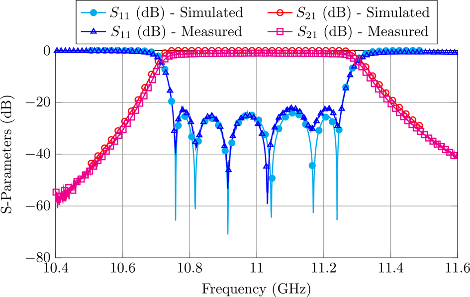
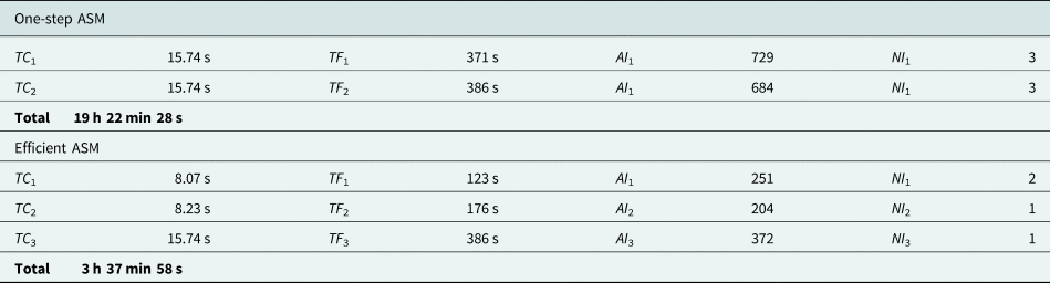
Table 2 shows the evolution of the design parameters in the Efficient ASM process. As it can be seen, only two or three variables are optimized in each step. Once we have designed half of the filter, we can duplicate it obtaining a very good performance. The last ASM iteration (which considers all design variables) is very fast, since all elements are very close to their target. Figure 3 shows the performance of the final fine model compared to the measurements of the hardware. As we can see, the agreement is indeed excellent. The Efficient ASM just described is 1.83 times faster than OS-ASM described in the previous section [Reference Melgarejo, Guglielmi, Cogollos and Boria12] (see Table 3 for the details).
Measured and simulated response of the six-pole inductive filter.

Evolution of the design parameters for the inductive six-pole filter in the Efficient ASM process. The design variables are the widths of the apertures (their thickness is fixed to 3.5 mm) and the lengths of the resonators (their heights and widths are set to 9.525 and 19.95 mm). All dimensions are in mm

Performance of both design methods for the in-line six-pole inductive waveguide filter

Dual-mode filter
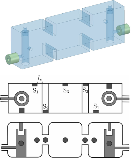
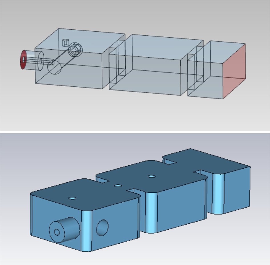
The second application example that we discuss is a more complex five-pole dual-mode filter [Reference San-Blas, Guglielmi, Melgarejo, Coves and Boria22]. The dual mode resonator exploits the resonance of a metallic post, together with the resonance of the rectangular cavity that contains the post. The filter is centered at 10 GHz, and has a bandwidth of 300 MHz. Figure 4 (top) shows the ideal coarse model of the filter.
Top: Coarse model of the five-pole filter with sharp corners, and without tuning elements (Fig. 1 from [Reference San-Blas, Guglielmi, Melgarejo, Coves and Boria22]). Bottom and center: Fine model of the filter with rounded corners and tuning elements (Fig. 26 from [Reference San-Blas, Guglielmi, Melgarejo, Coves and Boria22]).

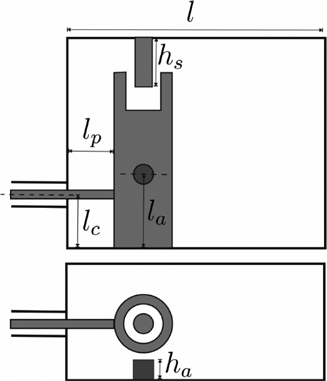
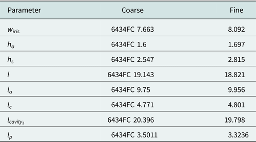
As already mentioned, there are two modes resonating in both the first and last cavities. The two resonances are the second resonance of the (re-entrant) post and the first resonance of the rectangular metallic enclosure. The dimensions of both the post and the metallic enclosure are chosen so that the two resonances occur at the same frequency (degenerate modes). The filter will again be manufactured using milling. The fine model must, therefore, include rounded corners (2 mm radius). In addition, it must also include tuning elements (0.9 mm radius) set at a fixed depth of 1 mm. Figure 4 (bottom) shows the fine model of the filter. The design parameters are the lengths of the cavities, the widths of the inductive irises (their thickness is fixed at 2 mm), together with the additional design variables shown in Fig. 5, namely, the height of the re-entrant post (h s), the height and offset of the cylinder that couples the two degenerate modes (h a and l a), the offset of the input/output coaxial port of the filter (l c), and the length of the connection from the coaxial port to the post (l p).
Dimensions that are optimized in the design process (Fig. 15 from [Reference San-Blas, Guglielmi, Melgarejo, Coves and Boria22]).

The coarse model is again simulated with FEST3D. However, in order to simulate the re-entrant post, FEST3D uses a module based on the well-known 3D Boundary Integral-Resonant Mode Expansion (BI-RME) method [Reference Arcioni, Bozzi, Bressan, Conciauro and Perregrini23]. As a result, the simulation is not as fast as the one of the inductive filter we discussed in the previous section. The high precision model is simulated, in this case, using CST. In order to achieve numerical convergence, we increased the density of CST's default initial mesh and let the adaptive mesh perform 24 iterations (using around 1 500 000 tetrahedrons).
OS-ASM
The first step in the design process is to obtain the dimensions of the coarse model (low accuracy) in Fig. 4 (top) that produces the desired response. This can be done, for instance, following the approach described in [Reference Guglielmi and Melcon21]. Due to the complexity of the hardware, however, it is more convenient to start directly with a two-pole rather than with a one-pole structure. Once the low accuracy two-pole structure is optimized, the complete filter can be assembled, and the central cavity optimized to get the desired response. A global optimization is also necessary to obtain a perfectly compliant set of dimensions for the coarse model.
Once the coarse model has been fully defined, we can start the OS-ASM design of the fine model. In this case, however, it is more convenient to proceed in two stages: in the first one we consider the tuning elements, and in the second one we add the rounded corners. The complete procedure is as follows:
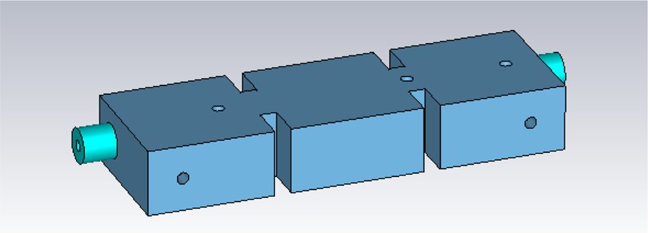
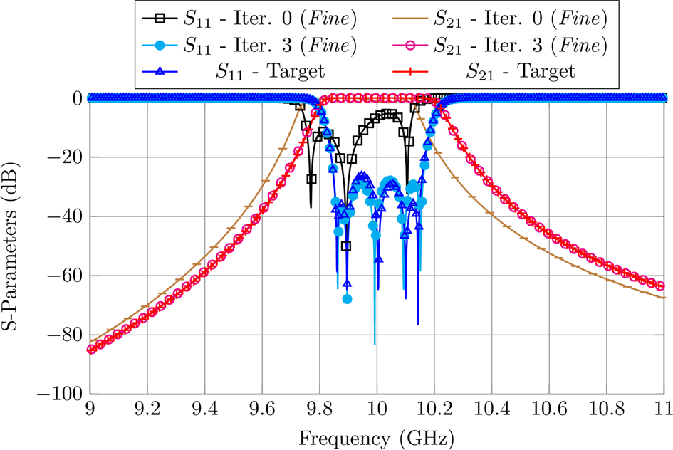
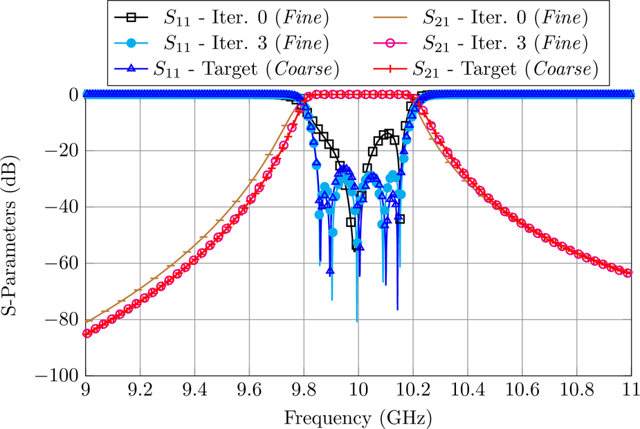
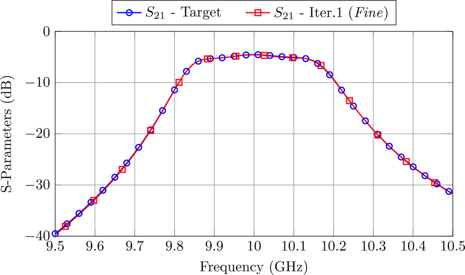
(i) Add first the tuning elements to the fine model (see Fig. 6) using, at the start of the procedure, the structural dimension of the coarse model. After three ASM iterations, both models provide a very similar response (see Fig. 7). It is important to note that, if we had included at this stage also the rounded corners, the initial performance of the fine model would have been too different from the target, and the coarse model would have required a significantly longer time to recover the performance of the fine model.
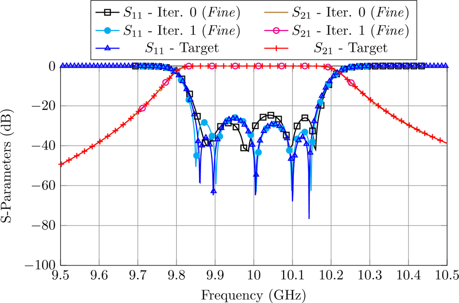
(ii) We can now add the rounded corners to the fine model, obtaining the structure shown in Fig. 4 (bottom). After three more ASM iterations, the fine model gives the desired target response (see Fig. 8).
Fine model of the filter that includes tuning elements.

ASM process to recover the desired performance of the fine model that includes tuning elements.

ASM process to recover the desired performance in the fine model including both tuning elements and rounded corners.

The overall time required to design the five-pole dual-mode filter using this approach can be computed as:


where TC i and TF i are the computation times of the coarse and fine models, NI i is the number of ASM iterations performed, and AI i is the average number of simulations it takes a simplex algorithm to recover each of the fine model responses.
Efficient ASM
In this case, the segmentation of the problem into smaller optimization spaces is more challenging. This is because the first cavity includes already six out of the total eight design variables. And, furthermore, the six variables are not completely independent. However, the segmentation strategy can still increase significantly the efficiency of the design process with respect to the one described in the previous section. The proposed approach is as follows:
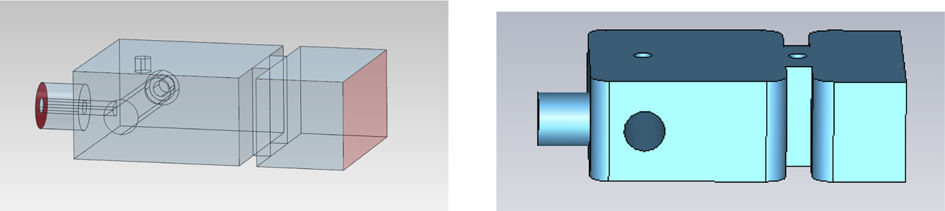
(i) The first step is again to generate a coarse model of the complete first cavity, including the coaxial input, the first cavity (with all its elements) and the first iris (see Fig. 9 left). This model can be rapidly optimized to obtain the desired two-pole performance.
(ii) The next step is to build the fine model of the first cavity including all tuning elements and rounded corners (see Fig. 9 right).
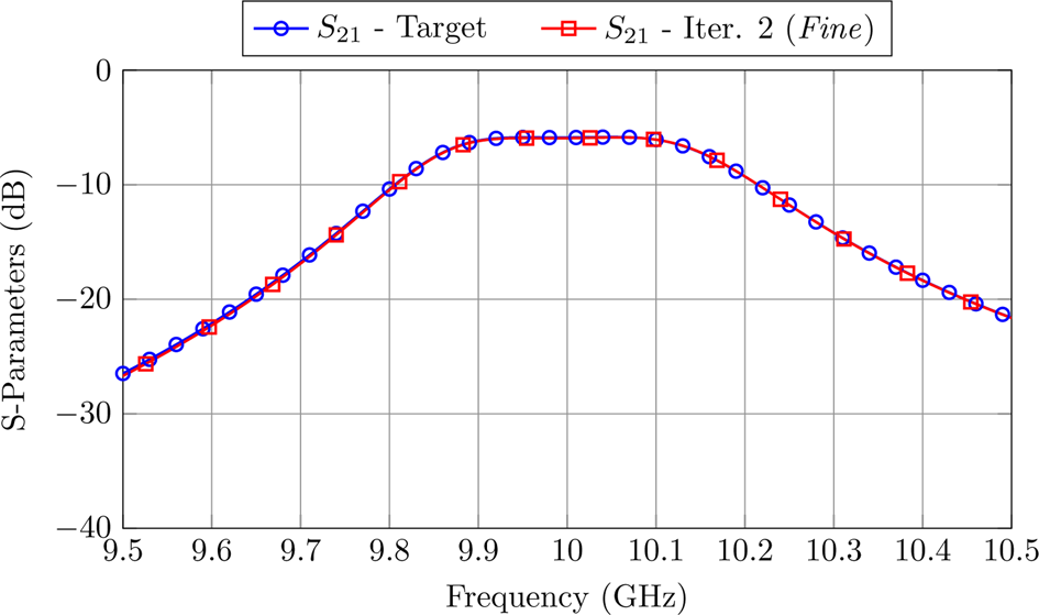
(iii) We can now use the OS-ASM method to align the coarse and the fine models. After two ASM iterations, both models provide the same performance (see Fig. 10). It is important to note that, even if we are optimizing seven parameters (all the dimensions from Fig. 9), the reduced coarse model is twice as fast as the coarse model of the complete filter.
(iv) We then add the central cavity to the coarse model and optimize the structure to obtain the required three-pole performance.
(v) Add next the central resonator and iris to the fine model, obtaining the second fine model shown in Fig. 11 (bottom). Perform one ASM iteration optimizing, primarily but not exclusively, the newly added elements. Figure 12 shows the performances of the fine and coarse models after the ASM process.
(vi) Finally, duplicate the first dual-mode cavity of the fine model to obtain the complete structure of the filter (Fig. 4, bottom). After only one ASM iteration with all the design parameters, the high precision model gives the desired performance (see Fig. 13).
First reduced model of the filter. Left: coarse model. Right: fine model.

ASM process to recover the desired performance in the first reduced fine model.

Top: Second coarse models of the filter. Bottom: Second fine model of the filter.

ASM process to recover the desired performance in the second reduced fine model.

Final performance of the fine model compared to its target.

The overall time required to design the five-pole band-pass filter is computed as:


This is 5.3 times faster than the method described in the previous section. Table 4 shows the time parameters of each procedure. It is therefore clear that, using the step-by-step approach based on partial models of the filter can always reduce very significantly the overall time required to obtain the desired target performance with the fine model. Table 5 shows the optimal dimensions for the coarse and fine models.
Performance of both design methods for the five-pole filter based on dual-mode coaxial resonators


Tuning techniques
Having successfully designed high precision models of our filters, we now need to move to the next phase, namely, tuning the filters after they have been manufactured. In this context, we first discuss a robotic tuner that we have developed to facilitate the tuning process. We then discuss two different tuning procedures: an ASM-based technique, and another approach that is based on available tuning knowledge.
Tuning robot
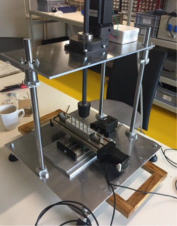
One issue that is important to note is that, in order to tune a filter, we must be able to control very precisely the motion and the position of all tuning elements. To do that, in a controllable and systematic way, we have built a simple precision robotic tuner, as shown in Fig. 14. The robotic tuner has three parts: a movable X-Y table to which the filter is fastened, a precision rotating arm with an actuator that can be coupled to the tuning elements, and three drivers connected to a PC to control the tuning process. The rotating arm is driven by a stepper motor with 800 steps for revolution. In addition, there is a 1:30 reduction gear. The resulting theoretical (minimal) uncertainty is 0.015 degrees. However, we have observed that, in practice, the angular accuracy of the system is about one degree. Taking into account that the pitch of the tuning elements is 0.397 mm, this results in a penetration accuracy of about one μm. This is enough to tune a large variety of filters.
Precision robotic tuner that we have built to control the tuning process.

ASM-based tuning procedure
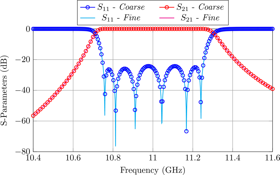
The first tuning procedure is based on ASM [Reference Melgarejo, Guglielmi, Cogollos and Boria19]. As usual, this technique uses two simulation models: the fine model shown in the top of Fig. 1, and the coarse model shown in the bottom of Fig. 1, respectively. The starting point of the tuning procedure is, in fact, what we know at the end of the filter design process, namely, that both the coarse and the fine model are aligned with the desired performance (Fig. 15). Furthermore, in the vicinity of the alignment point, we know that relation between the two models (or spaces) is given by (1), where it is important to recall that:
• xf refers to the penetrations of the tuners in the fine model shown in Fig. 1 (top).
• xc refers to the waveguide dimensions of the coarse model shown in Fig. 1 (bottom).
Aligned performances of the coarse and fine models of the inductive filter.

To proceed, we now need to compute the B matrix in (1). To do that, we now modify, one at the time, the penetration of each tuner of the fine model (indicated by xfi) and optimize instances of the coarse model to recover the fine model performances (xci). After doing that, following the procedure detailed in [Reference Melgarejo, Ossorio, Cogollos, Guglielmi, Boria and Bandler20], we can easily compute the elements of the matrix B that relates the filter dimensions of the coarse model with the penetrations of the tuning elements. Now that we have a good estimation of the B matrix at the point of alignment, we can proceed with the tuning process, as follows:
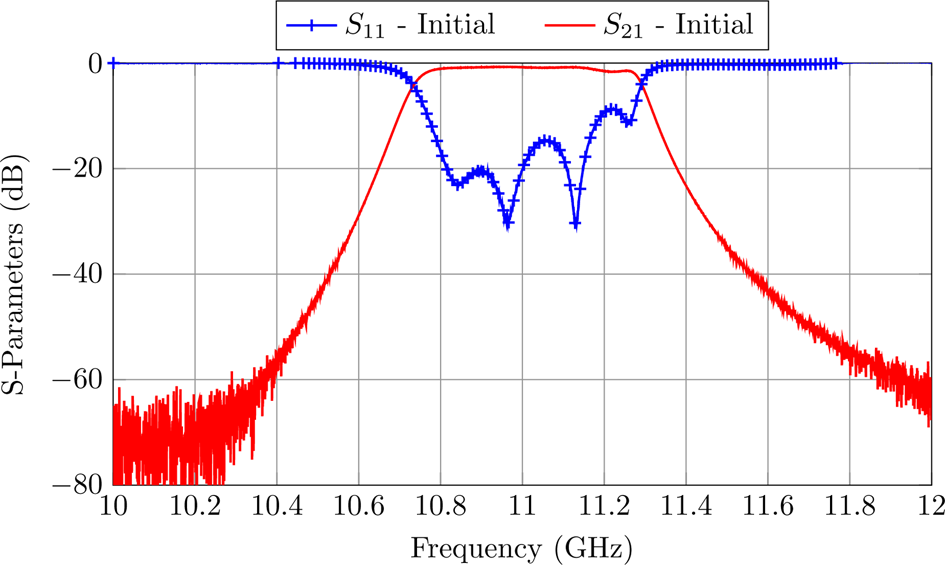
(i) Once the filter is manufactured, set the tuners at their design penetration (given by x1). This will provide, in our case, the response shown in Fig. 16, which we will refer to as R m(x1).
(ii) Optimize an instance of the coarse model until we recover the same performance, namely:
(9)$$R_c ( {\bf x_{cm}}) = R_m ( {\bf x_1}) $$(iii) Set the tuners of the filter to:
(10)$${\bf x_2} = {\bf x_1} + {\bf B} \cdot ( {\bf {x_c}_{opt}} - {\bf x_{cm}}) $$(iv) Go back to step (i) and repeat this process until the filter is completely tuned.


Performance of the filter when all tuning elements are set to the design depth.

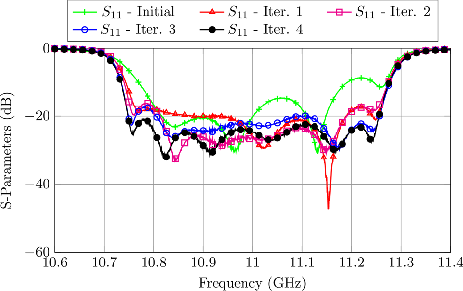
After four ASM iterations, our filter is successfully tuned as shown in Fig. 17.
Filter performance after every ASM iteration.

A knowledge-based approach
The ASM-based technique we just discussed could also be used for tuning the dual-mode filter. However, due to the relatively long simulation time that is required in this case (about 15 s for a single run), and the expected number of coarse simulations in each ASM iteration (about 600–700), the use of the ASM-based tuning technique would require a total of about 10–11 h.
We therefore propose to apply a different knowledge-based tuning approach. Our objective has been, in fact, to develop a semi-automatic tuning approach that is based on the manual tuning procedure that is widely used in the industrial environment. A key step in this context is to use Matlab to read the measurements of a VNA so that they can be further processed to support the tuning process. The resulting procedure is then as follows:
(i) Define first the S11 and S21 tuning masks. In this case, the return loss between 9.85 and 10.15 GHz should be lower than − 30 dB, and the S21 at 9.6 and 10.53 GHz should have minimum attenuation level of − 40 dB. The S11 error at each point is then computed using the following expression:
(11)$${e_{s_{11}}}^{( i) } = \left\{\matrix{ RL_{goal} - RL^{( i) },\; \hfill & \text{if}\ RL^{( i) } < RL_{\it goal} \hfill \cr 0,\; \hfill & \text{otherwise} \hfill }\right.$$and the S21 error is defined as:(12)$${e_{s_{21}}}^{( i) } = \left\{\matrix{ IL_{goal} - IL^{( i) },\; \hfill & \text{if}\ IL^{( i) } < IL_{\it goal} \hfill \cr 0,\; \hfill & \text{otherwise} \hfill }\right.$$The total error is then computed as:(13)$$E = {w_1 \over n_1} \sum_{i = 1}^{n_1} {e_{s_{11}}}^{( i) } + {w_2 \over n_2} \sum_{i = 1}^{n_2} {e_{s_{21}}}^{( i) },\; $$where w 1 and w 2 are the weights for the S11 and S21 terms, and n 1 and n 2 are the number of points used in each mask.(ii) The next step is to set all tuners to the design penetration.
(iii) We can then start the actual tuning procedure that consists of finding the penetration of each tuning element that minimizes the total error that we have just defined. A key step is now to define the order in which the tuners must be modified.
(iv) Following the guidelines from [Reference Lindner and Biebl24], we will first act upon the tuners in the cavities and then we will adjust the tuners that control the couplings. After each tuner movement, the error is recomputed using Matlab to decide if the movement must be kept or discarded (i.e., to return to the original position).
(v) This process is repeated until the filter is tuned, and all masks are satisfied.


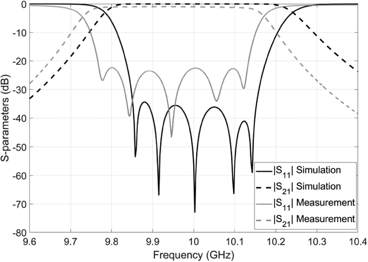
Figure 18 shows the performance of the filter at the end of the tuning process. As we can see, the performance that we have obtained is good but is not in perfect agreement with the simulations. Further investigations indicated that this disagreement is due to the dimensional errors introduced by the manufacturing process, in particular, with respect to the input and output couplings [Reference San-Blas, Guglielmi, Melgarejo, Coves and Boria22]. Our tuning procedure, however, was able to obtain, with a very reasonable effort, the best possible performance that the hardware could give. Finally, it is important to note that the successful use of the procedure just described does not require any previous tuning experience.
Final performance of the filter after the tuning process.

Conclusions
To reduce the costs of microwave filters, it is common practice to use a manufacturing technique that can deliver an intermediate (low cost) accuracy, like milling for instance, together with tuning elements that can be adjusted after manufacturing in order to obtain the desired filter performance. An inevitable consequence of this choice is that the presence of rounded corners and tuning elements must be included in the design process. This, in turn, can result in a significantly increased EM simulation effort. In this context, therefore, we have discussed in this paper two efficient design strategies that can be used to significantly decrease the computational effort to design microwave filters commonly used for both ground and space applications. In addition to filter design strategies, we have also discussed two systematic procedures to support the filter tuning stage.
The value of this contribution is, in our opinion, that the material discussed can, in fact, be considered as an end-to-end guide enabling young engineers to deliver compliant microwave filter designs with a minimum of previous experience.
Acknowledgments
This work was supported by funds from “La Caixa” Foundation (Code: LCF/BQ/DE17/11600013), and from the Ministry of Science and Innovation through the sub-projects C41 and C43 of the coordinated project PID2019-103982RB.
 Juan Carlos Melgarejo received a degree in Telecommunications, a double master in Telecommunications and a Ph.D. from the Universitat Politècnica de València in 2015, 2019, and 2021, respectively. His main research interests are design and optimization of complex waveguide filters.
 Javier Ossorio received a degree and, double master in Telecommunications Engineering and a Ph.D. from the Universitat Politècnica de València, Spain, in 2014, 2017 and 2021, respectively. His current research activities include EM simulations of waveguide filters, efficient design, optimizations, and development of new tunable filter structures for satellite applications.
 Ángel Antonio San-Blas received the Ingeniero de Telecomunicación degree and the Doctor Ingeniero de Telecomunicación degree from the Universitat Politècnica de València, Valencia, Spain, in 2000 and 2008, respectively. His current research interests include the analysis and design of passive waveguide components for satellite communication systems.
 Marco Guglielmi received the degree “Laurea in Ingegneria Elettronica” in 1979 from the University of Rome “La Sapienza”, Rome, Italy. In 1982, he obtained an M.S. Degree in Electrical Engineering from the University of Bridgeport, Bridgeport, Connecticut, USA. In 1986, he received a Ph.D. degree in Electrophysics from the Polytechnic University, Brooklyn, New York, USA. Dr. Guglielmi is currently holding the position of Invited Senior Researcher at the Polytechnic University of Valencia, Valencia, Spain. His main research interests are the development of electromagnetic simulation tools, microwave filters, and technology innovation management.
 Vicente E. Boria received the Doctor Ingeniero de Telecomunicación degree from Universidad Politécnica de Valencia, Spain, in 1997; where he is Full Professor since 2003. He leads the Microwave Applications Group, focused in the areas of EM-based analysis, design, and high-power modeling of microwave passive components (with special emphasis on filters and multiplexers).