2.1. Compliant wall model

In accordance with the work of Carpenter & Garrad (Reference Carpenter and Garrad1985) and Alexander et al. (Reference Alexander, Kirk and Papageorgiou2020), we prefer the same wall model to replicate the compliant substrate used by them, i.e. the compliant substrate consists of an isotropic impermeable elastic plate/tensorial membrane over a rigid substrate supported by an array of springs, as shown in figure 2. In fact, the array of springs is assembled in such a way that the wavelength of the surface instability is considerably larger in comparison with the distance between neighbouring springs. Furthermore, the cavity between the elastic plate and the rigid substrate is filled by a viscous fluid of different density and viscosity from the mainstream fluid flowing over the elastic plate, and it is referred to as the substrate fluid. It is assumed that deformations of the springs have negligible impact on the substrate fluid. As a consequence, the following linear equation is used to describe the deflection, $\eta (x,t)$, of the compliant substrate from its equilibrium position (Carpenter & Garrad Reference Carpenter and Garrad1985; Alexander et al. Reference Alexander, Kirk and Papageorgiou2020)

(2.9)\begin{equation} \rho_wb\partial_{tt}\eta+D\partial_t\eta+B\partial_{xxxx}\eta-T\partial_{xx}\eta+K\eta=p_s-p+2\mu[\partial_yv-(\partial_yu+\partial_xv)\partial_x\eta], \end{equation}

where $\rho _w$ is the density of the elastic material, $b$ is the thickness of the elastic plate, $D$ is the damping coefficient, $B$ is the flexural rigidity of the elastic plate, $T$ is the longitudinal tension, $K$ is the spring stiffness, $p_s$ is the pressure of the substrate fluid and $d_s$ is the equilibrium height of the substrate fluid. In fact, the flexural rigidity $B$ and the damping coefficient $D$ are not independent wall parameters. Instead, both can be measured from the material properties of the compliant substrate (Carpenter & Garrad Reference Carpenter and Garrad1985; Alexander et al. Reference Alexander, Kirk and Papageorgiou2020)

(2.10a,b)\begin{equation} B=\frac{E_Yb^3}{12(1-\nu^2)},\quad D=2\zeta \sqrt{K \rho_w b}, \end{equation}

where $E_Y$ is Young's modulus, $\nu$ is the Poisson ratio of the elastic material and $\zeta$ is the damping ratio. It should be useful to mention here that the viscous effect of the substrate fluid is neglected (Carpenter & Garrad Reference Carpenter and Garrad1985; Alexander et al. Reference Alexander, Kirk and Papageorgiou2020). However, the viscous effect pertaining to the mainstream fluid is included in (2.9) through the normal stress balance at the elastic plate, $y=\eta (x,t)$. For the sake of simplicity, $p_s$, the pressure of the substrate fluid with equilibrium height $d_s$, is assumed to be constant, although the elastic plate will undergo an infinitesimal deformation from its equilibrium position owing to the infinitesimal perturbation of the mainstream flow (Alexander et al. Reference Alexander, Kirk and Papageorgiou2020). In addition, velocity components of the mainstream fluid must satisfy no-slip and kinematic conditions at the compliant substrate, $y=\eta (x,t)$, (Matar et al. Reference Matar, Craster and Kumar2007; Peng et al. Reference Peng, Jiang, Zhuge and Zhang2016; Yang et al. Reference Yang, Jiang, Hu and Peng2018)

(2.11a,b)\begin{equation} u=0,\quad v=\partial_t\eta. \end{equation}

Figure 2.

Schematic diagram of a compliant substrate, where $b$ is the thickness of the elastic plate which is supported by an array of springs.

2.2. Base flow solution

As we are interested in deciphering the primary instability of a uni-directional surfactant-laden shear-imposed parallel flow with constant layer thickness $d$ of the mainstream fluid, constant surfactant concentration $\varGamma (x,t)=\varGamma _b$ and without compliant substrate deformation $\eta =0$, the governing equations (2.1)–(2.11a,b) are simplified according to the above assumptions and reduced to the following form:

(2.12a,b)\begin{gather} \mu \partial_{yy}u+\rho g \sin \theta =0,\quad \partial_yp+\rho g \cos \theta=0, \end{gather}

(2.13a,b)\begin{gather} \mu \partial_yu = \tau_s,\quad p=p_a,\quad \textrm{at}\ y=d, \end{gather}

(2.14a,b)\begin{gather} u = 0,\quad p=p_s,\quad \textrm{at}\ y=0. \end{gather}

The analytical solution of the base flow (2.12a,b)–(2.14a,b) can be expressed in non-dimensional form as

(2.15)\begin{equation} \left. \begin{gathered} U(y)=(2y-y^2)+\tau y,\quad P(y)=P_a+2\cot\theta(1-y),\ V=0,\\ \varGamma_e=1,\ H=1, \quad \eta=0,\ P_s=P_a+2\cot\theta, \end{gathered} \right\} \end{equation}

where the velocity at the surface of the mainstream fluid, $U_s=\rho g d^2\sin \theta /(2\mu )$, of the uni-directional parallel flow without shear is preferred as the characteristic velocity scale, the constant layer thickness $d$ of the mainstream fluid for the parallel flow is preferred as the characteristic length scale, $\mu U_s/d$ is preferred as the characteristic pressure scale, $d/U_s$ is preferred as the characteristic time scale, the base surfactant concentration $\varGamma _b$ is preferred as the characteristic scale for surfactant concentration and the base surface tension $\sigma _b$ is preferred as the characteristic scale for surface tension (Wei Reference Wei2005). Here, $\tau =\tau _sd/(\mu U_s)$ is the non-dimensional imposed shear stress, $P_a$ is the non-dimensional ambient pressure, $H$ is the non-dimensional mainstream fluid layer thickness of the unperturbed parallel flow and $\varGamma _e$ is the non-dimensional surfactant concentration in the case of unperturbed parallel flow. Note that the streamwise base velocity of the mainstream fluid is explicitly dependent on the imposed shear stress $\tau$. But, its maximum value no longer appears at the surface of the mainstream fluid owing to the presence of external shear stress.

3.1. Long-wave analysis

In order to investigate the primary instability governed by (3.12)–(3.20) in the long-wave regime ($k \sim 1/\lambda \to 0$, where $\lambda$ is the wavelength of the infinitesimal disturbance), we propose the long-wave series expansion (Yih Reference Yih1963; Smith Reference Smith1990; Samanta Reference Samanta2019)

(3.21) \begin{equation} \left. \begin{aligned} \tilde{u}(y) & =\tilde{u}_0+k\tilde{u}_1+k^2\tilde{u}_2+\cdots,\quad\quad \tilde{h}=\tilde{h}_0+k\tilde{h}_1+k^2\tilde{h}_2+\cdots,\\ \tilde{v}(y) & =k\tilde{v}_1+k^2\tilde{v}_2+k^3\tilde{v}_3+\cdots,\quad \tilde{\eta}=\tilde{\eta}_0+k\tilde{\eta}_1+k^2\tilde{\eta}_2+\cdots,\\ \tilde{p}(y) & =\tilde{p}_0+k\tilde{p}_1+k^2\tilde{p}_2+\cdots,\quad\quad \tilde{\varGamma}=\tilde{\varGamma}_0+k\tilde{\varGamma}_1+k^2\tilde{\varGamma}_2+\cdots,\\ c & =\tilde{c}_0+k\tilde{c}_1+k^2\tilde{c}_2+\cdots. \end{aligned} \right\} \end{equation}

It should be useful to mention here that the long-wave series expansion (3.21) is valid in the limit $k \to 0$. Hence, only long-wave unstable modes can be captured very well by using the series expansion (3.21). In fact, in the limit $k \to 0$, the temporal growth rate $kc_i$ of the long-wave mode approaches zero. As soon as $k$ increases, the series expansion (3.21) is not valid due to the convergence issue, and thereby, the unstable modes raised in the finite wavenumber regime cannot be obtained by using the long-wave series expansion. However, the long-wave series expansion (3.21) is very pertinent to determine the critical Reynolds number analytically for the onset of primary instability induced by the long-wave mode. In order to find out the unstable modes in the arbitrary wavenumber regime, we will use the numerical method discussed in the next section.

3.2. Order-$O(k^0)$ analysis

Substituting (3.21) in the perturbation equations (3.12)–(3.20), we collect the leading-order equations, i.e. the equations of order $O(k^0)$

(3.22)\begin{gather} \partial_{yy}\tilde{u}_0=0,\quad \partial_y\tilde{p}_0=0,\quad 0 \le y \le 1, \end{gather}

(3.23)\begin{gather} \partial_y\tilde{u}_0+\tilde{h}_0\partial_{yy}U=0,\quad \tilde{p}_0-2 \cot \theta \tilde{h}_0=0,\quad \textrm{at}\ y=1, \end{gather}

(3.24)\begin{gather} C_K\tilde{\eta}_0+\tilde{p}_0-2\cot \theta \tilde{\eta}_0=0,\quad \tilde{u}_0+\partial_yU\tilde{\eta}_0 =0,\quad \textrm{at}\ y=0. \end{gather}

It should be useful to mention here that the capillary number $Ca$ is assumed to be of order one, i.e. $Ca \sim O(1)$. For this reason, the capillary number is not manifested in the leading-order normal stress boundary condition. After solving the leading-order equations (3.22)–(3.24), the solution can be expressed as

(3.25)\begin{gather} \tilde{u}_0(y)=\left[2\tilde{h}_0y-(2+\tau)\tilde{\eta}_0\right],\quad \tilde{p}_0(y)=2\cot\theta \tilde{h}_0, \end{gather}

(3.26)\begin{gather}\tilde{\eta}_0={-}\left[\frac{2\cot\theta}{(C_K - 2\cot\theta)}\right]\tilde{h}_0={-}\left[\frac{2\cot\theta/C_K}{(1 - 2\cot\theta/C_K)}\right]\tilde{h}_0, \end{gather}

provided $C_k \neq 2\cot \theta =C_K^{*}$, the critical value of spring stiffness $C_K$. It should be noted that, for a given value of $\theta \neq 0$, $\tilde {\eta }_0 \rightarrow 0$ in the limit $C_K \to \infty$, or, $\theta \to {\rm \pi}/2$ when $\tilde {h}_0 \neq 0$. Therefore, the leading-order compliant substrate deformation is out of phase (in phase) with the leading-order fluid surface deformation if $C_K> C_K^{*}\ (< C_K^*)$ and $0 <\theta < {\rm \pi}/2$. Obviously, the streamwise velocity for the leading-order disturbed shear flow is linear in cross-stream coordinate $y$, and it explicitly depends on the external shear stress $\tau$ and spring stiffness $C_K$, the only wall parameter from the compliant substrate contributing to the leading-order disturbed shear flow. 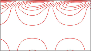However, the streamwise velocity for the leading-order shear flow will increase (decrease) if the leading-order compliant substrate deformation is out of phase (in phase) with the leading-order fluid surface deformation ($\tilde {h}_0>0$) and when the imposed shear stress is exerted in the co-flow direction ($\tau >0$). This physical fact is demonstrated in figure 3. In particular, the leading-order disturbed shear flow procures energy from the base flow through the perturbation tangential stress balance equation, but it modifies significantly in the presence of compliant substrate and imposed shear stress.

Figure 3.

(a) Here, $\tilde {h}_0$ is in phase with $\tilde {\eta }_0$ but out of phase with $\tilde {\varGamma }_0$ when $C_K < 2\cot \theta =C_K^*$. (b) Here, $\tilde {h}_0$ is out of phase with $\tilde {\eta }_0$ but in phase with $\tilde {\varGamma }_0$ when $C_K > 2\cot \theta =C_K^*$ and when the imposed shear stress acts in the co-flow direction ($\tau >0$). Here, $\tilde {u}_0(y)$ is the leading-order streamwise velocity for the disturbed fluid flow.

3.3. Order-$O(k^1)$ analysis

Now we collect the first-order equations, i.e. the equations of order $O(k^1)$

(3.27)\begin{gather} \textrm{i}\tilde{u}_0+\partial_y\tilde{v}_1=0,\quad 0 \le y \le 1, \end{gather}

(3.28)\begin{gather} Re[\textrm{i}(U-\tilde{c}_0)\tilde{u}_0+\partial_yU\tilde{v}_1]+\textrm{i}\tilde{p}_0-\partial_{yy}\tilde{u}_1=0,\quad 0 \le y \le 1, \end{gather}

(3.29)\begin{gather} \partial_y\tilde{p}_1-\partial_{yy}\tilde{v}_1=0,\quad 0 \le y \le 1, \end{gather}

(3.30)\begin{gather} \partial_y\tilde{u}_1+\tilde{h}_1\partial_{yy}U+\textrm{i}Ma\tilde{\varGamma}_0=0,\quad \textrm{at}\ y=1, \end{gather}

(3.31)\begin{gather} -\tilde{p}_1+2 \cot \theta \tilde{h}_1+2\partial_y\tilde{v}_1-2\textrm{i}\partial_yU\tilde{h}_0=0,\quad \textrm{at}\ y=1, \end{gather}

(3.32)\begin{gather} \textrm{i}(U-\tilde{c}_0)\tilde{\varGamma}_0+\textrm{i}\tilde{u}_0+\textrm{i}\partial_yU\tilde{h}_0=0,\quad \textrm{at}\ y=1, \end{gather}

(3.33)\begin{gather} \textrm{i}(U-\tilde{c}_0)\tilde{h}_0-\tilde{v}_1=0,\quad \textrm{at}\ y=1, \end{gather}

(3.34)\begin{gather} -\textrm{i}C_D\tilde{c}_0\tilde{\eta}_0+C_K\tilde{\eta}_1+\tilde{p}_1-2\cot \theta \tilde{\eta}_1-2[\partial_y\tilde{v}_1-\partial_yUi\tilde{\eta}_0]=0,\quad \textrm{at}\ y=0, \end{gather}

(3.35)\begin{gather} \tilde{u}_1+\partial_yU\tilde{\eta}_1 =0,\quad \textrm{at}\ y=0, \end{gather}

(3.36)\begin{gather} \tilde{v}_1+i\tilde{c}_0\tilde{\eta}_0=0,\quad \textrm{at}\ y=0. \end{gather}

After solving the first-order equations (3.27)–(3.36), one obtains the solution in the following form:

(3.37)\begin{gather} \widetilde{u_1}=\tilde{h}_0\left[\textrm{i}\,Re\left\{\tfrac{1}{12}(2+\tau) y^4-\tfrac{1}{3}\tilde{c}_0y^3-\tfrac{1}{3}(2+\tau)y+\tilde{c}_0y\right\}+\textrm{i}\,\cot\theta( y^2-2y)\right]+2\tilde{h}_{1}y\nonumber\\ -\textrm{i}\,May\tilde{\varGamma}_{0}-\textrm{i}\,Re\left\{\tfrac{1}{12}(2+\tau)y^4-\tfrac{1}{3}\tilde{c}_0y^3-\tfrac{1}{3}(2+\tau)y+\tilde{c}_0y\right\}\tilde{\eta}_0-(2+\tau)\tilde{\eta}_1, \end{gather}

(3.38)\begin{gather} \tilde{v}_1={-}\textrm{i}\tilde{h}_0y^2+(2+\tau)i\tilde{\eta}_0y-\textrm{i}\tilde{\eta}_0\tilde{c}_0, \end{gather}

(3.39)\begin{gather} \tilde{p}_1={-}2\textrm{i}\tilde{h}_0y-2\textrm{i}\tilde{h}_0(1+\tau)+2\cot\theta\tilde{h}_1+2(2+\tau)i\tilde{\eta}_0, \end{gather}

(3.40)\begin{gather} \tilde{\eta}_1=\frac{-2\cot\theta \tilde{h}_1+\textrm{i}[2(1+\tau)\tilde{h}_0-2(2+\tau)\tilde{\eta}_0+C_D\tilde{c}_0\tilde{\eta}_0]}{(C_K-2\cot\theta)}. \end{gather}

The analytical calculation unveils the existence of two dominant temporal modes, the so-called surface mode and surfactant mode (Wei Reference Wei2005; Bhat & Samanta Reference Bhat and Samanta2018). As a consequence, the notations $c_s$ and $c_m$ will be used in the subsequent calculations for the complex wave speeds of the surface mode and surfactant mode, respectively. If the leading-order amplitude of fluid surface deformation is non-zero ($\tilde {h}_0 \neq 0$), the long-wave mode induced by deflection of the fluid surface is referred to as the surface mode. In this case, the phase speed of the surface mode can be obtained from the kinematic equation (3.33) and is given by

(3.41)\begin{equation} \tilde{c}_0=\tilde{c}_{0s}=2+\tau, \end{equation}

where the subscript notation ‘$s$’ is used for the surface mode. Obviously, at leading order, the surface mode travels with a speed that is explicitly dependent on the imposed shear stress $\tau$. In this case, the leading-order amplitude $\tilde {\varGamma }_0$ of perturbation surfactant concentration can be obtained from the surfactant transport equation (3.32) and is given by

(3.42)\begin{equation} \tilde{\varGamma}_0=(2+\tau)[\tilde{h}_0-\tilde{\eta}_0]=\left[\frac{(2+\tau)C_K}{(C_K-2\cot\theta)}\right]\tilde{h}_0 =\left[\frac{(2+\tau)}{(1-2\cot\theta/C_K)}\right]\tilde{h}_0. \end{equation}

Therefore, $\tilde {\varGamma }_0 \to (2+\tau )\tilde {h}_0$ in the limit $C_K \to \infty$ when $\tilde {h}_0 \neq 0$. If the imposed shear stress acts in the co-flow direction ($\tau >0$), the leading-order perturbation surfactant concentration will be in phase (out of phase) with the leading-order fluid surface deformation if $C_K>C_K^*\ (< C_K^*)$. This physical fact is fully opposite to the leading-order compliant substrate deformation (see figure 3). It is evident that the leading-order amplitude of perturbation surfactant concentration decreases (increases) on account of the deformation of compliant substrate when $\tilde {\eta }_0$ is in phase (out of phase) with $\tilde {h}_0 (>0)$. By contrast, if $\tilde {h}_0 = 0$ and $\tilde {\varGamma }_0 \neq 0$, a different long-wave mode from the surface mode appears due to the deflection of surfactant concentration, and it is referred to as the surfactant mode/Marangoni mode. In this case, the phase speed of the surfactant mode can be obtained from the surfactant transport equation (3.32) and is given by

(3.43)\begin{equation} \tilde{c}_{0m}=1+\tau, \end{equation}

where the subscript notation ‘$m$’ is used for the surfactant mode/Marangoni mode. It should be noted that the leading-order phase speed for the surface mode is greater than the leading-order phase speed for the surfactant mode. In other words, to leading order, the surfactant mode travels slower than the surface mode. Furthermore, the compliant substrate has no influence on the leading-order phase speeds for the surface mode and surfactant mode respectively.

3.4. Order-$O(k^2)$ analysis

Now we collect the second-order equations, i.e. the equations of order $O(k^2)$

(3.44)\begin{gather} \textrm{i}\,\tilde{u}_1+\partial_y\tilde{v}_2=0,\quad 0 \le y \le 1, \end{gather}

(3.45)\begin{gather} Re[\textrm{i}(U-\tilde{c}_0)\tilde{u}_1-\textrm{i}\tilde{c}_1\tilde{u}_0 +\partial_yU\tilde{v}_2]+\textrm{i}\tilde{p}_1-(\partial_{yy}\tilde{u}_2-\tilde{u}_0)=0,\quad 0 \le y \le 1, \end{gather}

(3.46)\begin{gather} Re\,\textrm{i}(U-\tilde{c}_0)\tilde{v}_1+\partial_y\tilde{p}_2-\partial_{yy}\tilde{v}_2=0,\quad 0 \le y \le 1, \end{gather}

(3.47)\begin{gather} \partial_y\tilde{u}_2+\textrm{i}\tilde{v}_1+\tilde{h}_2\partial_{yy}U+\textrm{i}\,Ma\tilde{\varGamma}_1=0,\quad \textrm{at}\ y=1, \end{gather}

(3.48)\begin{gather} -\tilde{p}_2+2 \cot \theta \tilde{h}_2+2\partial_y\tilde{v}_2-2\textrm{i}\partial_yU\tilde{h}_1+(1/Ca)\tilde{h}_0=0,\quad \textrm{at}\ y=1, \end{gather}

(3.49)\begin{gather} \textrm{i}(U-\tilde{c}_0)\tilde{\varGamma}_1-\textrm{i}\tilde{c}_1\tilde{\varGamma}_0 +\textrm{i}\tilde{u}_1+\textrm{i}\partial_yU\tilde{h}_1=0,\quad \textrm{at}\ y=1, \end{gather}

(3.50)\begin{gather} \textrm{i}(U-\tilde{c}_0)\tilde{h}_1-\textrm{i}\tilde{c}_1\tilde{h}_0-\tilde{v}_2=0,\quad \textrm{at}\ y=1, \end{gather}

(3.51)\begin{gather} -C_I\tilde{c}_0^2\tilde{\eta}_0-\textrm{i}C_D(\tilde{c}_0\tilde{\eta}_1+\tilde{c}_1\tilde{\eta}_0) +C_T\tilde{\eta}_0+C_K\tilde{\eta}_2+\tilde{p}_2-2\cot \theta \tilde{\eta}_2\nonumber\\ -2[\partial_y\tilde{v}_2-\textrm{i}\partial_yU\tilde{\eta}_1]=0,\quad \textrm{at}\ y=0, \end{gather}

(3.52)\begin{gather} \tilde{u}_2+\partial_yU\tilde{\eta}_2 =0,\quad \textrm{at}\ y=0, \end{gather}

(3.53)\begin{gather} \tilde{v}_2+\textrm{i}(\tilde{c}_0\tilde{\eta}_1+\tilde{c}_1\tilde{\eta}_0)=0,\quad \textrm{at}\ y=0. \end{gather}

3.5. Surface mode

After solving the above second-order equations (3.44)–(3.53), $\tilde {u}_2$, $\tilde {v}_2$ and $\tilde {p}_2$ are determined and then, inserting the expression of $\tilde {v}_2$ in the kinematic equation (3.50), the expression of $\tilde {c}_1$ for the surface mode can be obtained as

(3.54)\begin{equation} \tilde{c}_1=\tilde{c}_{1s}=\textrm{i}\left[\frac{4}{15}(2+\tau)Re-\frac{2}{3}\cot \theta -\frac{1}{2}(2+\tau)Ma+\frac{4}{3} \frac{\cot^2\theta}{C_K}\right], \end{equation}

where the first term shows the destabilizing effect of inertia, the second term shows the stabilizing effect of depthwise gravity, the third term shows the stabilizing effect of insoluble surfactant and the fourth term shows the destabilizing effect of compliant substrate. Using the criterion for neutral stability ($c_i \approx kc_1=0$ as $k \to 0$), one can obtain the critical Reynolds number for the surface mode

(3.55)\begin{equation} Re_c=Re_{cs}=\frac{5}{2(2\!+\!\tau)}\cot \theta\!+\!\frac{15}{8}Ma-\frac{5}{(2\!+\!\tau)}\frac{\cot^2\theta}{C_K} =\frac{5\cot\theta}{2(2\!+\!\tau)}\left[1-\frac{2\cot\theta}{C_K}\right]+\frac{15}{8}Ma. \end{equation}

Obviously, the critical Reynolds number $Re_{cs}$ for the surface mode is modified by the Marangoni number $Ma$, imposed shear stress $\tau$ and spring stiffness $C_K$. However, it recovers the result of Alexander et al. (Reference Alexander, Kirk and Papageorgiou2020) very well in the absence of surface surfactant and imposed shear stress ($Ma \to 0$ and $\tau \to 0$). Furthermore, it coincides with the result of Wei (Reference Wei2005) as soon as the effect of a compliant substrate is ignored, i.e. if the spring stiffness $C_K \to \infty$. In fact, in leading order, the compliant substrate behaves as a rigid wall in the limit $C_K \to \infty$ (Alexander et al. Reference Alexander, Kirk and Papageorgiou2020). In particular, the critical Reynolds number $Re_{cs}$ for the surface mode enhances with the increasing value of Marangoni number. Hence, the Marangoni number, or equivalently, the insoluble surfactant, has a stabilizing effect on the surface mode (Wei Reference Wei2005). Further, if the imposed shear stress $\tau$ acts in the co-flow direction, the critical Reynolds number for the surface mode reduces with the increasing value of $\tau$ when the effect of the compliant substrate is neglected. Hence, the imposed shear stress has a destabilizing effect on the surface mode (Smith Reference Smith1990; Samanta Reference Samanta2014a). If the effect of the compliant substrate is incorporated, the critical Reynolds number for the surface mode reduces. Although, this reduction process of critical Reynolds number, or equivalently, the destabilizing effect of compliant substrate on the surface mode, can be weakened by gradually increasing the value of spring stiffness $C_K$ from its critical value $C_K^*=2\cot \theta$ ($C_K \neq C_K^*$). As discussed by Alexander et al. (Reference Alexander, Kirk and Papageorgiou2020), the surface mode will be always unstable in the absence of insoluble surfactant when $C_K< C_K^*$, because the critical Reynolds number for the surface mode approaches zero in the limit $C_K \to C_K^*$ and it becomes negative when $C_K< C_K^*$. But in the presence of insoluble surfactant, it is feasible to have a positive value of critical Reynolds number for the surface mode if the following condition for the Marangoni number $Ma$ is satisfied:

(3.56)\begin{equation} Ma > \frac{4\cot\theta}{3(2+\tau)}\left[\frac{2\cot\theta}{C_K}-1\right]=Ma^*, \end{equation}

when $C_K< C_K^*$ ($C_K \neq C_K^*$). Hence, for $Ma>Ma^*$, the critical value of the Marangoni number, there exists a stable range of Reynolds number where the primary instability induced by the surface mode can be made stable even though $C_K< C_K^*$. Otherwise, the infinitesimal disturbance will be unstable if $Ma < Ma^*$ when $C_K< C_K^*$. The above physical phenomenon is illustrated in figure 4. Indeed, the curve for $Re_{cs}$ approaches zero in the limits $C_K \to C_K^*=2$, $Ma \to 0$ and $\tau \to 0$, specified by a solid line. However, $Re_{cs}$ no longer becomes zero at $C_K=C_K^*$ as soon as the effect of Marangoni number ($Ma=1$) is included in the current flow model. Instead, the curve for $Re_{cs}$ intersects the $C_K$-axis at a lower value of $C_K$ than $C_K^*$, specified by a dashed line. Obviously, this new result is different from that of Alexander et al. (Reference Alexander, Kirk and Papageorgiou2020) where the insoluble surfactant is absent ($Ma=0$). Further, the interesting result is that the critical Reynolds number reduces (enhances) in the presence of imposed shear stress if $C_K > (< C_K^*)$, specified by dotted and dash-dotted lines, respectively. Hence, the imposed shear stress shows a dual role in the surface mode, i.e. a destabilizing effect when $C_K>C_K^*$ and a stabilizing effect when $C_K< C_K^*$.

Figure 4.

Variation of critical Reynolds number $Re_{cs}$ for the surface mode with the spring stiffness $C_K$ when $\theta =45^{\circ }$. Solid line represents the result when $Ma=0$ and $\tau =0$. Dashed line represents the result when $Ma=1$ and $\tau =0$. Dotted line represents the result when $Ma=1$ and $\tau =1$. Dash-dotted line represents the result when $Ma=1$ and $\tau =2$. Points are the results of Alexander et al. (Reference Alexander, Kirk and Papageorgiou2020).

3.6. Surfactant mode

After solving the above second-order equations (3.44)–(3.53) and inserting the expression of $\tilde {u}_1$ in the surfactant transport equation (3.49), the expression of $\tilde {c}_1$ for the surfactant mode can be written as

(3.57)\begin{equation} \tilde{c}_1=\tilde{c}_{1m}=\textrm{i} \left[\frac{\tau Ma}{2}\right]. \end{equation}

As discussed by Wei (Reference Wei2005) and Bhat & Samanta (Reference Bhat and Samanta2018), there exists an unstable surfactant mode in the presence of imposed shear stress $\tau$ for a surfactant-laden fluid flow, and it can be made stronger by increasing the values of imposed shear stress and Marangoni number. Further, from the second-order analytical calculation, one can report that the Reynolds number $Re$, or equivalently, the inertia, has no impact on the expression of the first-order temporal growth rate ($kc_i \propto c_1$ as $k \to 0$) for the surfactant mode. In addition, it is evident that the temporal growth rate for the surfactant mode is not influenced by the compliant substrate either.

3.7. Order-$O(k^3)$ analysis

Now we collect the third-order equations, i.e. the equations of order $O(k^3)$

(3.58)\begin{gather} \textrm{i}\tilde{u}_2+\partial_y\tilde{v}_3=0,\quad 0 \le y \le 1, \end{gather}

(3.59)\begin{gather} Re[\textrm{i}(U-\tilde{c}_0)\tilde{u}_2-\textrm{i}\tilde{c}_1\tilde{u}_1-\textrm{i}\tilde{c}_2\tilde{u}_0+\partial_yU\tilde{v}_3]+\textrm{i}\tilde{p}_2-(\partial_{yy}\tilde{u}_3 -\tilde{u}_1)=0,\quad 0 \le y \le 1, \end{gather}

(3.60)\begin{gather} Re[\textrm{i}(U-\tilde{c}_0)\tilde{v}_2-\textrm{i}\tilde{c}_1\tilde{v}_1]+\partial_y\tilde{p}_3-(\partial_{yy}\tilde{v}_3-\tilde{v}_1)=0,\quad 0 \le y \le 1, \end{gather}

(3.61)\begin{gather} \partial_y\tilde{u}_3+\textrm{i}\tilde{v}_2+\tilde{h}_3\partial_{yy}U +\textrm{i}Ma\tilde{\varGamma}_2=0,\quad \textrm{at}\ y=1, \end{gather}

(3.62)\begin{gather} -\tilde{p}_3+2 \cot \theta \tilde{h}_3+2\partial_y\tilde{v}_3-2\textrm{i}\partial_yU\tilde{h}_2+(1/Ca)\tilde{h}_1=0,\quad \textrm{at}\ y=1, \end{gather}

(3.63)\begin{gather} \textrm{i}(U-\tilde{c}_0)\tilde{\varGamma}_2-\textrm{i}\tilde{c}_1\tilde{\varGamma}_1-\textrm{i}\tilde{c}_2\tilde{\varGamma}_0+\textrm{i}\tilde{u}_2+\textrm{i}\partial_yU\tilde{h}_2=0,\quad \textrm{at}\ y=1, \end{gather}

(3.64)\begin{gather} \textrm{i}(U-\tilde{c}_0)\tilde{h}_2-\textrm{i}\tilde{c}_1\tilde{h}_1-\textrm{i}\tilde{c}_2\tilde{h}_0 -\tilde{v}_3=0,\quad \textrm{at}\ y=1, \end{gather}

(3.65)\begin{gather} -C_I(\tilde{c}_0^2\tilde{\eta}_1+2\tilde{c}_0\tilde{c}_1\tilde{\eta}_0)-\textrm{i}C_D(\tilde{c}_0\tilde{\eta}_2+\tilde{c}_1\tilde{\eta}_1+\tilde{c}_2\tilde{\eta}_0)+C_T\tilde{\eta}_1+C_K\tilde{\eta}_3\nonumber\\ +\tilde{p}_3-2\cot \theta \tilde{\eta}_3-2[\partial_y\tilde{v}_3-\textrm{i}\partial_yU\tilde{\eta}_2]=0,\quad \textrm{at}\ y=0, \end{gather}

(3.66)\begin{gather} \tilde{u}_3+\partial_yU\tilde{\eta}_3 =0,\quad \textrm{at}\ y=0, \end{gather}

(3.67)\begin{gather} \tilde{v}_3+\textrm{i}(\tilde{c}_0\tilde{\eta}_2+\tilde{c}_1\tilde{\eta}_1 +\tilde{c}_2\tilde{\eta}_0)=0,\quad \textrm{at}\ y=0. \end{gather}

After solving the third-order equations (3.58)–(3.67), $\tilde {u}_3$, $\tilde {v}_3$ and $\tilde {p}_3$ are determined and then, inserting the expressions of $\tilde {v}_3$ and $\tilde {u}_2$ in the kinematic equation (3.64) and surfactant transport equation (3.63), the expressions of $\tilde {c}_2$ for the surface mode and surfactant mode can be respectively obtained as

(3.68)\begin{gather} \tilde{c}_{2}=\tilde{c}_{2s}={-}2\left(1+\frac{\tau}{3}\right)+\left(\frac{40}{63}+\frac{7\tau}{36}\right) Re\cot\theta\left\{1-\frac{2\cot\theta}{C_K}\right\}\nonumber\\ \quad -\left(\frac{32}{63}+\frac{205\tau}{504} +\frac{11\tau^2}{144}\right)Re^2\nonumber\\ +\left(\frac{1}{6}+\frac{\tau}{3}\right)Ma\cot\theta\left \{1-\frac{2\cot\theta}{C_K}\right\}+\left(\frac{5}{6}+\frac{5\tau}{12}\right) Ma\,Re+\left(\frac{\tau}{2}+\frac{\tau^2}{4}\right)Ma^2\nonumber\\ + \left[\left(\frac{2}{3}+\frac{\tau}{3}\right)+\left\{\frac{2}{3}-\frac{(2+\tau)C_D}{3}\right\} \frac{2\cot\theta}{C_K}\right]\frac{2\cot\theta}{C_K}, \end{gather}

(3.69)\begin{gather} \tilde{c}_{2}=\tilde{c}_{2m}={-}\left(\frac{1}{6}+\frac{\tau}{3}\right)Ma\cot\theta \left\{1-\frac{2\cot\theta}{C_K}\right\}-\left(\frac{\tau}{2}+\frac{\tau^2}{4}\right)Ma^2. \end{gather}

It should be noted that the effect of the damping coefficient $C_D$ is now introduced in the expression for $\tilde {c}_{2s}$ for the surface mode. On the other hand, the expression of $\tilde {c}_{2m}$ for the surfactant mode is modified by the spring stiffness $C_K$, the only contribution being from the compliant substrate. Furthermore, the above expressions for $\tilde {c}_{2s}$ and $\tilde {c}_{2m}$ coincide with the results of Bhat & Samanta (Reference Bhat and Samanta2019) when the influence of the compliant substrate is neglected. The little differences in non-dimensional parameters are the consequence of the choice of various dimensionless scales. Similarly, solving the fourth-order ($O(k^4)$) equations, we obtain the expressions of $\tilde {c}_{3s}$ and $\tilde {c}_{3m}$ for the surface mode and surfactant mode respectively (see Appendix A). Obviously, the expression of $\tilde {c}_{3m}$ for the surfactant mode is explicitly dependent on $Re$, $C_K$ and $C_D$. Using the various-order solutions, the expression of the complex wave speed $c$ for the surface mode and surfactant mode can be respectively written as

(3.70)\begin{gather} c=c_s=\tilde{c}_{0s}+k\tilde{c}_{1s}+k^2\tilde{c}_{2s}+k^3\tilde{c}_{3s}+O(k^4) =c_{r}+\textrm{i}c_{i}, \end{gather}

(3.71)\begin{gather}c=c_m=\tilde{c}_{0m}+k\tilde{c}_{1m}+k^2\tilde{c}_{2m}+k^3\tilde{c}_{3m}+O(k^4) =c_{r}+\textrm{i}c_{i}, \end{gather}

where $c_{r}$ and $kc_{i}$ specify the phase speed and temporal growth rate of the infinitesimal disturbance, respectively. Therefore, based on the long-wave analysis, one can claim that the inertia, or equivalently the Reynolds number $Re$, has a weak effect on the temporal growth rate for the surfactant mode because the effect of $Re$ appears in the expression of order $O(k^3)$. Next, the long-wave results will be produced based on (3.70) and (3.71). In order to confirm the dual behaviour of the imposed shear stress on the surface mode in two distinct regimes of $C_K$ ($C_K< C_K^*$ & $C_K>C_K^*$), we compute the temporal growth rate for the surface mode when the imposed shear stress varies. Figure 5 demonstrates the variation of temporal growth rate $kc_i$ with wavenumber $k$ for the surface mode. It is observed that the temporal growth rate for the surface mode attenuates with the increasing value of $\tau$ when $C_K < C_K^*$, but it enhances with the increasing value of $\tau$ when $C_K>C_K^*$. These facts fully ensure the dual role of imposed shear stress in the surface mode and are consistent with the results reported in figure 4. Hence, the imposed shear stress has a stabilizing effect on the surface mode when $C_K< C_K^*$. However, it shows a destabilizing effect on the surface mode when $C_K>C_K^*$. Further, in order to confirm the stabilizing effect of the Marangoni number on the surface mode, we produce the temporal growth rate again for the surface mode when the Marangoni number varies rather than $\tau$. The result can be found in figure 6. In this case, the temporal growth rate for the surface mode attenuates in both regimes of $C_K$ ($C_K< C_K^*$ & $C_K>C_K^*$) as soon as the Marangoni number increases. The above results ensure the stabilizing effect of the Marangoni number on the surface mode. Hence, for a surfactant-laden fluid flowing down a compliant substrate, one can obtain a stable range of Reynolds number for the surface mode when $C_K < C_K^*$. Furthermore, in order to analyse the effects of wall parameters $C_K$ and $C_D$ on the surfactant mode, the temporal growth rate for the surfactant mode is plotted in figure 7. Note that the temporal growth rate for the surfactant mode enhances with increasing values of spring stiffness $C_K$ and damping coefficient $C_D$. Hence, both spring stiffness and damping coefficient exhibit a destabilizing effect on the surfactant mode. Apparently, it seems that the effect of $C_K$ is more discernible than that of $C_D$ on the surfactant mode. Basically, in the presence of flexible substrate, a non-zero first-order longitudinal fluid velocity component $\tilde {u}_1$ is generated in the case of the surfactant mode. This fact is different from the study of surfactant-laden shear-imposed flow over a rigid substrate (Wei Reference Wei2005; Bhat & Samanta Reference Bhat and Samanta2019), where first-order velocity components of the perturbation fluid are identically zero for the surfactant mode. As a result, in the present case, the additional longitudinal shear flow boosts the shear-induced Marangoni instability through the perturbation tangential stress balance equation and yields a destabilizing effect.

Figure 5.

(a) Variation of temporal growth rate $kc_i$ with wavenumber $k$ for the surface mode when $Re=1$ and $C_K=1< C_K^*$. Solid, dashed and dotted lines stand for $\tau =0.1$, $\tau =0.2$ and $\tau =0.3$ respectively. The arrow shows the direction of decreasing temporal growth rate with increasing $\tau$. (b) Variation of temporal growth rate $kc_i$ with wavenumber $k$ for the surface mode when $Re=2.5$ and $C_K=3>C_K^*$. Solid, dashed and dotted lines stand for $\tau =0.1$, $\tau =0.2$ and $\tau =0.3$, respectively. The arrow shows the direction of increasing temporal growth rate with increasing $\tau$. The other parameter values are $C_I=C_D=C_T=0$, $Ca=2$, $Ma=1$ and $\theta =45^{\circ }$. The results are plotted by solving (3.70).

Figure 6.

(a) Variation of temporal growth rate $kc_i$ with wavenumber $k$ for the surface mode when $Re=1$ and $C_K=1< C_K^*$. Solid, dashed and dotted lines stand for $Ma=0.8$, $Ma=0.9$ and $Ma=1.0$, respectively. The arrow shows the direction of decreasing temporal growth rate with increasing $Ma$. (b) Variation of temporal growth rate $kc_i$ with wavenumber $k$ for the surface mode when $Re=1$ and $C_K=3>C_K^*$. Solid, dashed and dotted lines stand for $Ma=0.1$, $Ma=0.2$ and $Ma=0.3$ respectively. The arrow shows the direction of decreasing temporal growth rate with increasing $Ma$. The other parameter values are $C_I=C_D=C_T=0$, $Ca=2$, $\tau =0.1$ and $\theta =45^{\circ }$. The results are plotted by solving (3.70).

Figure 7.

(a) Variation of temporal growth rate $kc_i$ with wavenumber $k$ for the surfactant mode when $C_D=1$. Solid, dashed and dotted lines stand for $C_K=0.5$, $C_K=0.6$ and $C_K=0.7$ respectively. The arrow shows the direction of increasing temporal growth rate with increasing $C_K$. (b) Variation of temporal growth rate $kc_i$ with wavenumber $k$ for the surfactant mode when $C_K=0.5$. Solid, dashed and dotted lines stand for $C_D=1$, $C_D=1.25$ and $C_D=1.5$ respectively. The arrow shows the direction of increasing temporal growth rate with increasing $C_D$. The other parameter values are $Re=0.1$, $Ca=2$, $Ma=0.1$, $\tau =0.1$ and $\theta =45^{\circ }$. The results are plotted by solving (3.71).

4.1. Validation of the numerical code

Before producing the current results, the numerical code is validated with the available results of the literature. Consequently, we choose the parameter values as given in Alexander et al. (Reference Alexander, Kirk and Papageorgiou2020) $C_I=1$, $C_D=1$, $C_B=1$, $C_T=1$, $Ca=1$, $Ma=0$, $\tau =0$ and $\theta =45^{\circ }$. Figure 8 exhibits the neutral curve and temporal growth rate for the surface mode when the wall parameter $C_K$ alters. It should be noted that the current results capture the results of Alexander et al. (Reference Alexander, Kirk and Papageorgiou2020) very well in appropriate limits, i.e. when the flow parameter values are the same as specified in Alexander et al. (Reference Alexander, Kirk and Papageorgiou2020). Apparently, it seems that there occurs subcritical instability in the finite wavenumber regime with a decreasing value of spring stiffness $C_K$, i.e. the finite wavelength instability induced by the surface mode may occur before criticality obtained from the long-wave analysis (see figure 8a). In particular, the primary instability for the given parameter values begins at $C_K=5$ when the Reynolds number exceeds its critical value. As soon as $C_K$ decreases, the finite wavelength subcritical instability generated by the surface mode occurs at a lower Reynolds number than the critical Reynolds number. If $C_K$ is further reduced ($C_K=2.6$), the finite wavelength instability even takes place at zero Reynolds number. In this case, we have found an unstable range of finite wavenumber where instability occurs despite the value of zero Reynolds number, which indicates the existence of inertialess instability induced by the surface mode in the finite wavenumber regime (the discussion of inertialess instability analysis can be found in Appendix B). The associated unstable region magnifies with the decreasing value of $C_K$. The above results are also confirmed through the plot of temporal growth rate demonstrated in figure 8(b). Obviously, there exists an unstable range of finite wavenumber at $C_K=2.6$, where the temporal growth rate is positive, as expected. Moreover, the temporal growth rate intensifies with the decreasing value of $C_K$ and supports the result reported in figure 8(a). Hence, the increasing value of $C_K$ has a stabilizing effect on the surface mode. In order to compare with the results acquired from the long-wave analysis, the critical Reynolds number for the surface mode is computed numerically and verified with that obtained from the long-wave analysis. Table 1 shows an excellent agreement between them. Moreover, it is observed that the critical Reynolds number for the surface mode enhances with the increasing value of $C_K$, which is fully consistent with the stabilizing effect of $C_K$ on the surface mode.

Figure 8.

(a) Variation of neutral curve for the surface mode in the ($Re$, $k$) plane for different values of $C_K$. Solid, dashed, dotted and dash-dotted lines stand for $C_K=5$, $C_K=3$, $C_K=2.6$ and $C_K=2$ respectively. The arrow shows the direction of decreasing unstable region with increasing $C_K$. (b) Variation of temporal growth rate $kc_i$ with wavenumber $k$ for the surface mode when $Re=0.2$. Solid, dashed, dotted and dash-dotted lines stand for $C_K=2.6$, $C_K=2.4$, $C_K=2.2$ and $C_K=2$ respectively. The arrow shows the direction of decreasing temporal growth rate with increasing $C_K$. The other parameter values are $C_I=1$, $C_D=1$, $C_B=1$, $C_T=1$, $Ca=1$, $Ma=0$, $\tau =0$ and $\theta =45^{\circ }$. Here, $U$ and $S$ represent unstable and stable regions. Points are the results of Alexander et al. (Reference Alexander, Kirk and Papageorgiou2020). The results are plotted by solving the eigenvalue problem (4.10).

Table 1.

Analytical and numerical comparison of critical Reynolds number for the surface mode when $C_K$ varies. The other parameter values are $C_I=1$, $C_D=1$, $C_B=1$, $C_T=1$, $Ca=1$, $Ma=0$, $\tau =0$ and $\theta =45^{\circ }$.

Following Alexander et al. (Reference Alexander, Kirk and Papageorgiou2020), if a particular set of wall parameters ($C_I=1$, $C_B=1$, $C_T=1$, $C_K=5$, $C_D=0.32$) is preferred in the numerical simulation, a new temporal mode, the so-called wall mode, appears in the ($Re$, $k$) plane (see figure 9a). It should be noted that the primary instability induced by the wall mode emerges in the finite wavenumber regime instead of the long-wave regime, and the unstable domain responsible for the wall mode magnifies with the decreasing value of $C_D$. Hence, the increasing value of damping coefficient $C_D$ has a stabilizing effect on the wall mode. Moreover, the primary instability generated by the wall mode occurs even at zero Reynolds number when $C_D=0.3$, which indicates the existence of inertialess instability induced by the wall mode in the finite wavenumber regime. In order to strengthen the above result, the temporal growth rate for the wall mode is also computed numerically and illustrated in figure 9(b) when $C_D$ varies. Obviously, the temporal growth rate attenuates as soon as $C_D$ increases and ensures the stabilizing effect of $C_D$ on the wall mode. To take into account the effect of $C_K$ on the wall mode, the numerical simulation is again performed when the wall parameter $C_K$ varies while $C_D=0.32$ is fixed. The associated result is depicted in figure 10(a). Note that the unstable domain for the wall mode reduces with the increasing value of $C_K$, and this fact is followed by the successive increment of critical Reynolds number. Hence, increasing spring stiffness $C_K$ shows a stabilizing effect on the wall mode as predicted by the damping coefficient $C_D$ on the wall mode. Figure 10(b) displays the associated temporal growth rate for the wall mode when $C_K$ alters. Obviously, the maximum temporal growth rate attenuates with the increasing value of $C_K$, which is fully consistent with the result reported in figure 10(a). As discussed by Alexander et al. (Reference Alexander, Kirk and Papageorgiou2020), the compliant substrate behaves gradually as a rigid substrate with increasing values of the wall parameters $C_K$ and $C_D$, which precludes the wall mode evolving with time, and is probably the reason for the stabilizing effects of $C_K$ and $C_D$ on the wall mode.

Figure 9.

(a) Variation of neutral curve for the wall mode in the ($Re$, $k$) plane for different values of $C_D$. Solid, dashed and dotted lines stand for $C_D=0.3$, $C_D=0.32$ and $C_D=0.34$ respectively. The arrow shows the direction of decreasing unstable region with increasing $C_D$. (b) Variation of temporal growth rate $kc_i$ with wavenumber $k$ for the wall mode when $Re=2$. Solid, dashed and dotted lines stand for $C_D=0.3$, $C_D=0.32$ and $C_D=0.34$ respectively. The arrow shows the direction of decreasing temporal growth rate with increasing $C_D$. The other parameter values are $C_I=1$, $C_K=5$, $C_B=1$, $C_T=1$, $Ca=1$, $Ma=0$, $\tau =0$ and $\theta =45^{\circ }$. Here, $U$ and $S$ represent unstable and stable regions. Points are the results of Alexander et al. (Reference Alexander, Kirk and Papageorgiou2020). The results are plotted by solving the eigenvalue problem (4.10).

Figure 10.

(a) Variation of neutral curve for the wall mode in the ($Re$, $k$) plane for different values of $C_K$. Solid, dashed and dotted lines stand for $C_K=5$, $C_K=7.5$ and $C_K=10$ respectively. The arrow shows the direction of decreasing unstable region with increasing $C_K$. (b) Variation of temporal growth rate $kc_i$ with wavenumber $k$ for the wall mode when $Re=3$. Solid, dashed and dotted lines stand for $C_K=5$, $C_K=7.5$ and $C_K=10$ respectively. The arrow shows the direction of decreasing temporal growth rate with increasing $C_K$. The other parameter values are $C_I=1$, $C_D=0.32$, $C_B=1$, $C_T=1$, $Ca=1$, $Ma=0$, $\tau =0$ and $\theta =45^{\circ }$. Here, $U$ and $S$ represent unstable and stable regions. Points are the results of Alexander et al. (Reference Alexander, Kirk and Papageorgiou2020). The results are plotted by solving the eigenvalue problem (4.10).

4.2. Effect of inclination angle on the wall mode

As the critical Reynolds number for the surface mode is determined analytically, which decreases with the increasing value of $\theta$, so the inclination angle has a destabilizing effect on the surface mode. On the other hand, the critical Reynolds number for the wall mode cannot be determined analytically based on the long-wave analysis because it appears in the finite wavenumber regime. Therefore, in order to examine the solo effect of inclination angle on the wall mode, $\theta$ is changed in the numerical simulation when other parameter values are fixed. Figure 11 illustrates the neutral curve and temporal growth rate for the wall mode when $\theta$ changes. It is observed that the unstable domain for the wall mode magnifies significantly with the increasing value of inclination angle, and this fact is followed by the successive reduction of the critical Reynolds number. Hence, the increasing value of inclination angle has a destabilizing effect on the wall mode, as speculated for the surface mode. In this case also, the primary instability induced by the wall mode occurs at zero Reynolds number when $\theta =50^{\circ }$. Hence, we can obtain an unstable range of finite wavenumber even at zero Reynolds number where the infinitesimal disturbance will be susceptible to instability by the wall mode. This result indicates the existence of inertialess instability generated by the wall mode in the finite wavenumber regime. Basically, the stabilizing influence of depthwise gravity on the primary instability weakens as soon as the inclination angle increases. This fact can be attributed to the cause for the destabilizing effect of inclination angle on the wall mode.

Figure 11.

(a) Variation of neutral curve for the wall mode in the ($Re$, $k$) plane for different values of $\theta$. Solid, dashed, dotted and dash-dotted lines stand for $\theta =35^{\circ }$, $\theta =40^{\circ }$, $\theta =45^{\circ }$ and $\theta =50^{\circ }$ respectively. The arrow shows the direction of the increasing unstable region with increasing $\theta$. (b) Variation of temporal growth rate $kc_i$ with wavenumber $k$ for the wall mode when $Re=3$. Solid, dashed, dotted and dash-dotted lines stand for $\theta =35^{\circ }$, $\theta =40^{\circ }$, $\theta =45^{\circ }$ and $\theta =50^{\circ }$ respectively. The arrow shows the direction of increasing temporal growth rate with increasing $\theta$. The other parameter values are $C_I=1$, $C_K=5$, $C_D=0.32$, $C_B=1$, $C_T=1$, $Ca=1$, $Ma=0$ and $\tau =0$. Here, $U$ and $S$ represent unstable and stable regions. The results are plotted by solving the eigenvalue problem (4.10).

4.3. Effect of Marangoni number on the surface mode and wall mode

In this subsection, we shall solely explore the effect of Marangoni number on the primary instabilities induced by the surface mode and wall mode. Consequently, we set $\tau =0$. In accordance with the work of Alexander et al. (Reference Alexander, Kirk and Papageorgiou2020), the parameter values are selected as $C_I=1$, $C_D=0.32$, $C_K=5$, $C_T=1$ and $\theta =45^{\circ }$. As discussed by Alexander et al. (Reference Alexander, Kirk and Papageorgiou2020), we have numerically found two dominant temporal modes, the so-called surface mode and wall mode, when the Reynolds number is low and the inclination angle is high. The associated neutral curves for the surface mode and wall mode are displayed in figure 12(a) when the Marangoni number varies. It is observed that the unstable region for the wall mode is enhanced but the unstable region for the surface mode is reduced with an increasing value of the Marangoni number. Hence, the Marangoni number has a destabilizing effect on the wall mode but shows a stabilizing effect on the surface mode. The interesting fact is that the instability for the wall mode occurs even at zero Reynolds number with the increasing value of Marangoni number. Therefore, one can claim that there exists inertialess instability induced by the wall mode at higher values of the Marangoni number. Further, the critical Reynolds number for the wall mode is lower than that for the surface mode. Hence, the finite wavenumber primary instability induced by the wall mode commences before the primary instability generated by the surface mode. As soon as the Reynolds number increases, the surface mode dominates the primary instability in the long-wave regime instead of the wall mode. This result indicates the existence of a mode switching process in the finite wavenumber regime. On the contrary, if the value of wall damping coefficient $C_D$ is slightly increased and set to $C_D=0.38$, the opposite phenomenon occurs, i.e. the critical Reynolds number for the surface mode is no longer higher than that for the wall mode. Instead, it is lower than that for the wall mode at $Ma=0$, which can be found in figure 12(b). Therefore, the primary instability is initially dominated by the surface mode rather than the wall mode when $Ma=0$ and $C_D=0.38$. If the Marangoni number is increased in the numerical simulation, the result again reverses at $Ma=0.6$, i.e. the critical Reynolds number for the wall mode is lower than that for the surface mode. It seems that there exists a competition between the wall mode and surface mode with the variation of parameter values to trigger the primary instability initially. In order to confirm the above results, the temporal growth rates for the surface mode and wall mode are revealed in figures 12(c) and 12(d) where $Re=2$ and $Re=0.6$, respectively. Obviously, the temporal growth rate for the surface mode becomes weaker while the temporal growth rate for the wall mode becomes stronger as soon as the Marangoni number increases. These results are fully in favour of the results reported in figure 12(a).

Figure 12.

(a) Variation of neutral curves for the surface mode and wall mode in the ($Re$, $k$) plane for different values of $Ma$ when $C_D=0.32$. Solid, dashed, dotted and dash-dotted lines stand for $Ma=0$, $Ma=0.1$, $Ma=0.2$ and $Ma=0.3$ respectively. (b) Variation of neutral curves for the surface mode and wall mode in the ($Re$, $k$) plane for different values of $Ma$ when $C_D=0.38$. Solid, dashed and dotted lines stand for $Ma=0$, $Ma=0.3$ and $Ma=0.6$ respectively. (c) Variation of temporal growth rate $kc_i$ with wavenumber $k$ for the surface mode when $Re=2$ and $C_D=0.32$. Solid, dashed, dotted and dash-dotted lines stand for $Ma=0$, $Ma=0.1$, $Ma=0.2$ and $Ma=0.3$ respectively. The arrow shows the direction of decreasing temporal growth rate with increasing $Ma$. (d) Variation of temporal growth rate $kc_i$ with wavenumber $k$ for the wall mode when $Re=0.6$ and $C_D=0.32$. Solid, dashed, dotted and dash-dotted lines stand for $Ma=0$, $Ma=0.1$, $Ma=0.2$ and $Ma=0.3$ respectively. The arrow shows the direction of increasing temporal growth rate with increasing $Ma$. The other parameter values are $C_I=1$, $C_K=5$, $C_B=1$, $C_T=1$, $Ca=1$, $\tau =0$ and $\theta =45^{\circ }$. Here, $U$ and $S$ represent unstable and stable regions. The results are plotted by solving the eigenvalue problem (4.10).

4.4. Effect of imposed shear stress on the surface mode and wall mode

In order to investigate the solo effect of imposed shear stress on the primary instabilities induced by the surface mode and wall mode, we set $Ma=0$, $C_K=5$ and $C_D=0.32$. Figure 13(a) displays the neutral curve in the ($Re$, $k$) plane when $\tau$ varies. It is observed that both the surface mode and wall mode appear in the neutral diagram as before. However, the unstable region for the surface mode is magnified while the unstable region for the wall mode decays with the increasing value of imposed shear stress. Hence, the imposed shear stress has a destabilizing effect on the surface mode but shows a stabilizing effect on the wall mode. This result is fully opposite to the effect of Marangoni number on the surface mode and wall mode. Furthermore, the critical Reynolds number for the surface mode is greater than that of the wall mode at $\tau =0$. Therefore, at the outset, the primary instability is dominated by the wall mode in the finite wavenumber regime. As soon as $\tau$ increases, the reverse phenomenon happens, i.e. the critical Reynolds number for the wall mode is greater than that of the surface mode at $\tau =0.2$. Hence, the primary instability is triggered by the surface mode at the outset instead of the wall mode when $\tau =0.2$. Again, the mode switching process takes place with the increasing value of imposed shear stress. If the wall damping coefficient $C_D$ is slightly shifted to a higher value $C_D=0.38$ as before, the primary instability is always dominated by the surface mode at the outset (see figure 13b). In this case, the wall mode has no chance to trigger the primary instability at the beginning, because the critical Reynolds number for the wall mode is always greater than that of the surface mode. Figures 13(c) and 13(d) demonstrate the associated temporal growth rates for the surface mode and wall mode, respectively. It should be noted that the temporal growth rate for the surface mode becomes stronger while the temporal growth rate for the wall mode becomes weaker in the presence of imposed shear stress. These results are fully consistent with the results reported in figure 13(a).

Figure 13.

(a) Variation of neutral curves for the surface mode and wall mode in the ($Re$, $k$) plane for different values of $\tau$ when $C_D=0.32$. Solid, dashed and dotted lines stand for $\tau =0$, $\tau =0.1$ and $\tau =0.2$ respectively. (b) Variation of neutral curves for the surface mode and wall mode in the ($Re$, $k$) plane for different values of $\tau$ when $C_D=0.38$. Solid, dashed and dotted lines stand for $\tau =0$, $\tau =0.1$, and $\tau =0.2$ respectively. (c) Variation of temporal growth rate $kc_i$ with wavenumber $k$ for the surface mode when $Re=1$ and $C_D=0.32$. Solid, dashed and dotted lines stand for $\tau =0$, $\tau =0.1$ and $\tau =0.2$ respectively. The arrow shows the direction of increasing temporal growth rate with increasing $\tau$. (d) Variation of temporal growth rate $kc_i$ with wavenumber $k$ for the wall mode when $Re=2$ and $C_D=0.32$. Solid, dashed and dotted lines stand for $\tau =0$, $\tau =0.1$ and $\tau =0.2$ respectively. The arrow shows the direction of decreasing temporal growth rate with increasing $\tau$. The other parameter values are $C_I=1$, $C_K=5$, $C_B=1$, $C_T=1$, $Ca=1$, $Ma=0$ and $\theta =45^{\circ }$. Here, $U$ and $S$ represent unstable and stable regions. The results are plotted by solving the eigenvalue problem (4.10).

4.5. Effect of wall parameters $C_I$, $C_T$ and $C_B$ on the surface mode and wall mode

In this subsection, we shall explore the effects of wall parameters $C_I$, $C_T$ and $C_B$ on the surface mode and wall mode, respectively. First, we shall vary the compliant substrate inertia, or equivalently, $C_I$ when other wall parameters are fixed. The results are displayed in figure 14(a). It should be noted that the unstable domain associated with the surface mode magnifies significantly with the increasing value of $C_I$. However, the critical Reynolds number from which the neutral curves emanate is the same for all neutral curves because the critical Reynolds number for the surface mode acquired from the long-wave analysis does not depend on the wall parameter $C_I$ (see (3.55)). Moreover, we can perceive the existence of subcritical instability with the increasing value of $C_I$. In particular, the primary instability generated by the surface mode occurs at $C_I=1$ when the Reynolds number exceeds its critical value. As soon as the wall parameter $C_I$ increases, the neutral curve distorts from its initial shape and exhibits subcritical instability at $C_I=2.4$. In this case, the primary instability responsible for the surface mode happens in the finite wavenumber regime even when the Reynolds number is lower than the critical value. If $C_I$ is further increased, the primary instability even takes place in the finite wavenumber regime despite the value of zero Reynolds number when $C_I=2.45$. Therefore, there exists inertialess instability induced by the surface mode in the finite wavenumber regime with the increasing value of $C_I$. On the other hand, the slight variation of $C_I$ has a significant impact on the wall mode. The result can be found in figure 14(b). It should be noted that the unstable region corresponding to the wall mode also magnifies with the increasing value of $C_I$. This fact is followed by the successive reduction of critical Reynolds number for the wall mode. Furthermore, there is possible to have inertialess instability in the finite wavenumber regime induced by the wall mode as well with the increasing value of $C_I$. Hence, the wall parameter $C_I$ has a destabilizing effect on the surface mode and wall mode. Figure 15 reveals the variation of neutral curves for the surface mode and wall mode when the wall parameters $C_T$ and $C_B$ change but $C_I$ is fixed. In both cases, the unstable domains associated with the surface mode and wall mode attenuate with the increasing values of $C_T$ and $C_B$ respectively. Therefore, both wall parameters $C_T$ and $C_B$ have a stabilizing effect on the surface mode and wall mode, respectively. It should be noted that the critical Reynolds number for the surface mode does not alter with the variations of $C_T$ and $C_B$. This fact is fully consistent with the analytical expression of critical Reynolds number for the surface mode supplied in (3.55). As the critical Reynolds number for the surface mode is fixed with the variations of wall parameters $C_T$ and $C_B$, there is a prospect for the surface mode to dominate the primary instability at the beginning with the increasing values of wall parameters $C_T$ and $C_B$ because the critical Reynolds number for the wall mode reduces successively as long as $C_T$ and $C_B$ increase.

Figure 14.

(a) Variation of neutral curve for the surface mode in the ($Re$, $k$) plane for different values of $C_I$. Solid, dashed, dotted, dash-dotted and thick lines stand for $C_I=1$, $C_I=1.5$, $C_I=2$, $C_I=2.4$ and $C_I=2.45$, respectively. The arrow shows the direction of the increasing unstable region with increasing $C_I$. (b) Variation of neutral curve for the wall mode in the ($Re$, $k$) plane for different values of $C_I$. Solid, dashed and dotted lines stand for $C_I=1$, $C_I=1.05$ and $C_I=1.1$, respectively. The arrow shows the direction of the increasing unstable region with increasing $C_I$. The other parameter values are $C_K=5$, $C_T=1$, $C_B=1$, $C_D=0.32$, $Ca=1$, $Ma=0$, $\tau =0$ and $\theta =45^{\circ }$. Here, $U$ and $S$ represent unstable and stable regions. The results are plotted by solving the eigenvalue problem (4.10).

Figure 15.

(a) Variation of neutral curves for the surface mode and wall mode in the ($Re$, $k$) plane for different values of $C_T$ when $C_B=1$. Solid, dashed and dotted lines stand for $C_T=1$, $C_T=3$ and $C_T=5$, respectively. (b) Variation of neutral curves for the surface mode and wall mode in the ($Re$, $k$) plane for different values of $C_B$ when $C_T=1$. Solid, dashed and dotted lines stand for $C_B=1$, $C_B=5$ and $C_B=10$, respectively. The other parameter values are $C_I=1$, $C_K=5$, $C_D=0.32$, $Ca=1$, $Ma=0$, $\tau =0$ and $\theta =45^{\circ }$. Here, $U$ and $S$ represent unstable and stable regions. The results are plotted by solving the eigenvalue problem (4.10).