2.1. Charges

Let X be a nonempty set and let ${\mathcal{P}}$ be an algebra on X. A probability charge, or simply charge, on $(X, {\mathcal{P}})$ is a function $\mu \colon {\mathcal{P}} \rightarrow [0,1]$ such that $\mu(X) = 1$ and, for all disjoint sets $E, F \in {\mathcal{P}}$ , $\mu (E \cup F) = \mu (E) + \mu (F)$ . A charge is thus finitely additive, but not necessarily countably additive. We denote the set of all charges on $(X, {\mathcal{P}})$ by $\mathcal{C}(X,{\mathcal{P}})$ , and use the notation $\mu(x)$ instead of $\mu( \{ x \} )$ .

When X is countably infinite, we say that $\mu \in \mathcal{C}(X, 2^X)$ is a diffuse charge if $\mu( x ) = 0$ for every $x \in X$ . Diffuse charges are not countably additive. It follows from the axiom of choice that diffuse charges exist (see, for example, Rao and Rao (Reference Rao and Rao1983), p. 38).

The following statement follows from Theorem 2 in Los and Marczewski (Reference Loś and Marczewski1949) together with the axiom of choice: If ${\mathcal{P}}$ is an algebra on X and $\mu$ is a charge on $(X,{\mathcal{P}})$ , then there exists a charge $\nu$ on $(X, 2^X)$ such that $\nu(E)=\mu(E)$ for all $E \in {\mathcal{P}}$ . We say that $\nu$ extends $\mu$ .

2.2. Integration with respect to charges

Let ${\mathcal{P}}$ be an algebra on X. A function $s \colon X \rightarrow \mathbb{R}$ is called a ${\mathcal{P}}$ -measurable simple function if $s = \sum_{i=1}^m c_i \mathbb{I}_{B_i}$ , where $c_1, \ldots, c_m \in \mathbb{R}$ , $\{B_1, \ldots, B_m\}$ is a ${\mathcal{P}}$ -measurable partition of X, and $\mathbb{I}_{B_i}$ is the characteristic function of the set $B_i$ . Let $\mu$ be a charge on $(X, {\mathcal{P}})$ . The integral of s with respect to $\mu$ is defined by $\int_{X} s % \mathrm{d} \mu = \sum_{i=1}^m c_i \cdot \mu(B_i)$ .

Let $\mu$ be a charge on $(X, {\mathcal{P}})$ . For a bounded function $f{\colon}X \rightarrow \mathbb{R}$ , the lower integral of f with respect to $\mu$ is defined as the supremum of all real numbers $\int_{X} s % \mathrm{d} \mu$ , where s is a ${\mathcal{P}}$ -measurable simple function with $s \le f$ . The upper integral of f is defined analogously. The function $f {\colon}X \rightarrow \mathbb{R}$ is called ${\mathcal{P}}$ -integrable if for each $\mu\in \mathcal{C}(X, {\mathcal{P}})$ , the lower and the upper integrals of f with respect to $\mu$ coincide. It follows from Theorems 4.5.7 and 4.7.3 in Rao and Rao (Reference Rao and Rao1983) that f is ${\mathcal{P}}$ -integrable if and only if for every ${\varepsilon}>0$ there exists a ${\mathcal{P}}$ -measurable simple function $f':P\rightarrow \mathbb{R}$ such that $|\,f(\,p)-f'(\,p)|\leq {\varepsilon}$ for every $p\in P$ . Consequently, any bounded function $f{\colon}X \rightarrow \mathbb{R}$ is $2^X$ -integrable. ${\mathcal{P}}$ -integrability is sometimes called uniform ${\mathcal{P}}$ -approachability of f. Similar conditions also appear for example in Section 4 of Marinacci (Reference Marinacci1997) and Section 2.1.3 of Harris et al. (Reference Harris, Stinchcombe and Zame2005), albeit in a different context. Notice that if the function f is ${\mathcal{P}}$ -integrable, then it is also ${\mathcal{P}}'$ -integrable for all ${\mathcal{P}}' \supset {\mathcal{P}}$ .

3.1. The decision problem

Let A be an action set having at least two elements. Let H denote the set of finite sequences in A, including the empty sequence $\phi$ . Let P denote the set of infinite sequences in A. Elements of A are called actions, elements of H are called histories, and elements of P are called plays. Let $u:P\rightarrow \mathbb{R}$ be a bounded function, called the payoff function.

Consider the following decision problem. At each period $t=1,2,\ldots$ , the decision maker chooses an action $a_t$ from A, knowing the previous choices $(a_1,\ldots,a_{t-1})\in H$ . This induces a play $p=(a_1,a_2,\ldots)$ . The payoff of the decision maker is $u(\,p)$ . (Note that the set of available actions does not depend on the history of the decision problem, and is always A. Moreover, notice that our model is equivalent to a model with a state variable and deterministic transitions.)

A strategy is a decision rule that gives a recommendation to the decision maker for choosing actions. These recommendations can be given in essentially different ways, and based on that we distinguish three different types of strategies: pure strategies, mixed strategies, and behavior strategies. We discuss each type of strategy in turn.

3.2. Pure strategies

A pure strategy is a function $f:H\rightarrow A$ . The interpretation is that if history h arises during the decision problem, then the strategy f recommends that the decision maker choose action f(h). Note that a pure strategy is completely deterministic.

Each pure strategy f induces a unique play $p_f$ . Of course, two different pure strategies can induce the same play, but any play can be generated by at least one pure strategy. We denote the set of pure strategies by F.

3.3. Mixed strategies

A mixed strategy is a charge $m\in\mathcal{C}(F, 2^F)$ on the set of pure strategies. The interpretation is that the decision maker should draw a pure strategy f according to m, and play the decision problem by using f. Note that a pure strategy can be seen as a mixed strategy that places probability 1 on this pure strategy.

3.4. Behavior strategies

A behavior strategy is a function $b:H\rightarrow \mathcal{C}(A,2^A)$ . The interpretation is that if history h arises during the decision problem, then the strategy b recommends that the decision maker choose an action according to the charge b(h).

Thus, a behavior strategy successively uses an infinite sequence of charges during the play. Consequently, a behavior strategy that places probability 1 on an action $a_t$ at every period t does not necessarily induce the play $(a_1,a_2,\ldots)$ with probability 1 in our finitely additive setting. So, a pure strategy cannot necessarily be identified with the behavior strategy placing probability 1 on the corresponding actions. This is in sharp contrast with the countably additive setup (see Section 6).

4.1. Mixed strategies

In this subsection we consider mixed strategies. First, we define the charge that a mixed strategy induces on a set of plays. This allows us to calculate the expected payoff for each mixed strategy and define optimal mixed strategies. Finally, we show that an optimal mixed strategy always exists.

A pure strategy f induces a unique play $p_f$ . Naturally, a mixed strategy m generates a charge $m^*$ on $(P,2^P)$ , given for every $Q \subseteq P$ by

(1) \begin{equation} m^*(Q) = m\,(\{\,f\in F: p_f\in Q\}). \label{eqn1} \end{equation}

Note that, as different pure strategies can induce the same play, different mixed strategies can induce the same charge on $(P,2^P)$ .

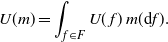
A pure strategy f induces the payoff $U(\,f)=u(\,p_f)$ . As a mixed strategy m prescribes drawing a pure strategy f according to the charge m defined on $(F,2^F)$ , the expected payoff for the mixed strategy m is given by

(2) \begin{equation} U (m) = \int_{f \in F} U (\,f)\; m({\rm d} f) . \label{eqn2} \end{equation}

The next lemma claims that the expected payoff for a mixed strategy can also be calculated through the induced charge on $(P,2^P)$ . The proof is straightforward and therefore omitted.

Lemma 1. For every mixed strategy m,

$$U (m) = \int_{p \in P} u (\,p) \;m^* ({\rm d} p).$$

We call a pure strategy f optimal if $U(\,f) = \sup_{p\in P}u(\,p)$ . Similarly, we call a mixed strategy m optimal if $U(m)=\sup_{p\in P}u(\,p)$ .

It is not always true that there exists a pure optimal strategy, since the payoff function u might not have a maximum, for example when the range of u is the set $\{1-1/n:n\in{\mathbb{N}}\}$ . However, it is easy to see that an optimal mixed strategy always exists.

Proof. Let $U^*=\sup_{p\in P} u(\,p)$ . For each $n\in\mathbb{N}$ , let $p_n\in P$ be a play such that $u(\,p_n)\geq U^*-\frac{1}{n}$ , and let $f_n$ denote a pure strategy that induces the play $p_n$ .

Let $\tau$ be a diffuse charge on $({\mathbb{N}}, 2^{{\mathbb{N}}})$ . Now consider the mixed strategy m that, intuitively, first chooses a natural number $n\in {\mathbb{N}}$ according to $\tau$ and then plays the pure strategy $f_{n}$ . Formally, for every subset F’ of the set F of pure strategies we have

\[m(F') = \tau(\{n\in{\mathbb{N}} \mid f_{n}\in F'\}).\]

Let $K\in {\mathbb{N}}$ . Since

\[m(\{\,f_K,f_{K+1},\ldots\}) = \tau(\{K,K+1,\ldots\})\;=\;1,\]

it follows from (2) that

\begin{align*} U(m)= \int_{f \in F} U (\,f)\; m({\rm d} f)= \int_{f \in \{\,f_K,f_{K+1},\ldots\}} U (\,f)\; m({\rm d} f)\geq U^*-\frac{1}{K} . \end{align*}

As this holds for every $K\in {\mathbb{N}}$ , we have $U(m)=U^*$ .

4.2. Behavior strategies

In this subsection we turn to behavior strategies. We consider algebras on the set of plays that satisfy a minimal richness condition. We call such algebras competent. Then, we define the charge that a behavior strategy induces on such a competent algebra. Based on these induced charges, we define optimal behavior strategies.

For a history $h \in H$ and a play $p \in P$ we use the notation $h \prec p$ if the play p starts with the history h. For two histories $h, h' \in H$ we use the notation $h \preceq h'$ if the history h’ starts with h (allowing $h'=h$ ), and use the notation $h \prec h'$ if h’ starts with h and h’ is strictly longer than h.

We now discuss the algebras that we consider on the set of plays. Arguably, a minimal requirement on the algebra is that it should contain all subsets of plays that are determined in finite time. More precisely, for every $n \in {\mathbb{N}}$ and $S \subseteq A^n$ , the algebra should contain the set

\[[S] = \{p\in P %\vert \exists \mid \text{there exists}\ h\in S\text{ with } h\prec p\}.\]

Thus, a play $p=(a_1,a_2,\ldots)$ belongs to [S], where $S \subseteq A^n$ , if and only if $(a_1,\ldots,a_n)$ belongs to S. For the special case when $S=\{(a_1,a_2,\ldots,a_n)\}$ is a singleton set, for convenience we write $[a_1,a_2, \ldots, a_n]$ instead of $[\{(a_1,a_2, \ldots, a_n)\}]$ .

Let ${\mathcal R}^{\rm f}$ denote the set of all sets [S], where $S \subseteq A^n$ for some $n\in{\mathbb{N}}$ . The superscript f refers to a finite horizon. The set $\mathcal{R}^{\rm f}$ consists of the so-called ‘finite-dimensional’ subsets of the set P of plays. The following statement is well known and easy to verify.

Lemma 2. ${\mathcal R}^{\rm f}$ is an algebra.

Take a behavior strategy b and a set [S], where $S\subseteq A^n$ for some $n\in {\mathbb{N}}$ . It is natural and standard to calculate the probability of the set [S] under b through n iterated integrals as follows: let

(3) \begin{align} c^{\rm f}(b)([S])=\int_{a_{1} \in A} \cdots \int_{a_n\in A} \mathbb{I}_{S}(a_1, \ldots, a_n)\ b(a_1, \ldots, a_{n-1}) ({\rm d} a_n)\cdots b(\oslash) ({\rm d} a_{1}) . \label{eqn3} \end{align}

Note that $c^{\rm f}(b)$ is a charge on the algebra ${\mathcal R}^{\rm f}$ . In the language of Dubins and Savage, $c^{\rm f}(b)([S])$ is nothing but the strategic probability of [S].

Definition 1. An algebra ${\mathcal{P}}$ of P is called competent if ${\mathcal{P}}\supseteq {\mathcal R}^{\rm f}$ . Given a competent algebra ${\mathcal{P}}$ , a ${\mathcal{P}}$ -specification is a function $\psi^{\mathcal{P}}$ that to each behavior strategy b assigns a charge $\psi^{\mathcal{P}}(b)$ on $(P,{\mathcal{P}})$ with the requirement that, for all sets $[S]\in {\mathcal R}^{\rm f}$ ,

$$\psi^{\mathcal{P}}(b)([S])\;=\;c^{\rm f}(b)([S]).$$

Thus, given a competent algebra ${\mathcal{P}}$ and a behavior strategy b, a ${\mathcal{P}}$ -specification $\psi^{\mathcal{P}}$ assigns a probability $\psi^{\mathcal{P}}(b)(R)$ to each set R in the algebra ${\mathcal{P}}$ , the only requirement being that $\psi^{\mathcal{P}}$ coincides with $c^{\rm f}$ on the algebra ${\mathcal R}^{\rm f}$ .

Note that ${\mathcal R}^{\rm f}$ , in view of Lemma 2, is a competent algebra of P, and $c^{\rm f}$ , defined in (3), is an ${\mathcal R}^{\rm f}$ -specification.

Let ${\mathcal{P}}$ be a competent algebra of P, and let $\psi^{\mathcal{P}}$ be a ${\mathcal{P}}$ -specification. Assume that the payoff function u is ${\mathcal{P}}$ -integrable. Then, for every behavior strategy b, the payoff function u has the same lower and upper integrals with respect to $\psi^{\mathcal{P}}(b)$ , which we denote by $U(b \mid {\mathcal{P}},\psi^{\mathcal{P}})$ . Based on this observation, we can define optimality for behavior strategies.

4.3. Equivalence of strategies

Consider a competent algebra ${\mathcal{P}}$ on P. Each mixed strategy m induces a charge $m^{\mathcal{P}}$ on $(P,{\mathcal{P}})$ , which is the restriction of the charge $m^*$ defined in (1) to the algebra ${\mathcal{P}}$ . Also, given a ${\mathcal{P}}$ -specification $\psi^{\mathcal{P}}$ , each behavior strategy b induces a charge $\psi^{\mathcal{P}}(b)$ on $(P,{\mathcal{P}})$ . This allows us to define equivalence between strategies.

According to the next theorem, we can find an equivalent mixed strategy for every behavior strategy under general conditions. The proof can be found in the Appendix.

The converse, when for a given mixed strategy we try to find an equivalent behavior strategy, is much more complicated. This is highlighted by a two-period decision problem in Section 2 of Dubins (Reference Dubins1975), with action space ${\mathbb{N}}$ at period 1 and only two actions at period 2. In this decision problem there is a mixed strategy for which there is no $({\mathcal R}^{\rm f}, c^{\rm f})$ -equivalent behavior strategy. This example is rather minimal, since for lack of equivalence at least two time periods are needed and in at least one time period there have to be infinitely many actions. For the proof Dubins refers to an implicit argument in de Finetti (Reference de Finetti1972). The following theorem follows directly from this example. Since our terminology is different, we provide a proof along the construction of Dubins (Reference Dubins1975).

Proof. For simplicity, assume that $\mathbb{N}\subseteq A$ . For each $n\in\mathbb{N}$ , consider pure strategies $f_n$ and $g_n$ that induce the plays $p_n=(n,1,1,\ldots)$ and $q_n=(n,2,2,\ldots)$ , respectively. Let $\tau^f$ be a diffuse charge on $(\mathbb{N},2^{{\mathbb{N}}})$ and let $\tau^g$ be the countably additive probability measure on $(\mathbb{N},2^{{\mathbb{N}}})$ with $\tau^g(n)=\frac{1}{2^n}$ for each $n\in\mathbb{N}$ .

Following Dubins (Reference Dubins1975), we define a mixed strategy m that, intuitively, gives a recommendation for a pure strategy in the following way: (1) with probability $\frac{1}{2}$ , it chooses $n\in\mathbb{N}$ according to $\tau^f$ and recommends the pure strategy $f_n$ ; and (2) with probability $\frac{1}{2}$ , it chooses $n\in\mathbb{N}$ according to $\tau^g$ and recommends the pure strategy $g_n$ .

More precisely, for every subset F’ of the set of pure strategies F we have

\[m(F') = \frac{1}{2}\cdot \tau^f(\{n\in\mathbb{N} \mid f_n\in F'\}) + \frac{1}{2}\cdot \tau^g(\{n\in\mathbb{N} \mid g_n\in F'\}).\]

This mixed strategy m does not have a $({\mathcal{P}},\psi^{\mathcal{P}})$ -equivalent behavior strategy for any competent algebra ${\mathcal{P}}$ and ${\mathcal{P}}$ -specification $\psi^{\mathcal{P}}$ . Indeed, suppose by way of contradiction that a behavior strategy b is $({\mathcal{P}},\psi^{\mathcal{P}})$ -equivalent to m for some competent algebra ${\mathcal{P}}$ and ${\mathcal{P}}$ -specification $\psi^{\mathcal{P}}$ .

Step 1. For every $W\in {\mathcal{P}}$ it holds that

\[m^*(W) = \frac{1}{2}\cdot \tau^f(\{n\in\mathbb{N} \mid p_n\in W\}) + \frac{1}{2}\cdot \tau^g(\{n\in\mathbb{N} \mid q_n\in W\}).\]

Consequently, we have the following under the mixed strategy m for every $n\in\mathbb{N}$ :

[1] The first action is n with probability

\[m^*([n]) = \frac{1}{2}\cdot \tau^f(n)+\frac{1}{2}\cdot \tau^g(n) = 0+\frac{1}{2^{n+1}} = \frac{1}{2^{n+1}}.\]

[2] The histories (n,1) and (n,2) have probability

\[m^*([n,1]) = \frac{1}{2}\cdot \tau^f(n) = 0\quad % \text{and}\quad % m^*([n,2]) = \frac{1}{2}\cdot \tau^g(n) = \frac{1}{2^{n+1}}.\]

Note that the sets [n], [n,1], and [n,2] belong to ${\mathcal{P}}$ , as the algebra ${\mathcal{P}}$ is competent.

Step 2. Since the behavior strategy b is $({\mathcal{P}},\psi^{\mathcal{P}})$ -equivalent to m, we have for every $n\in\mathbb{N}$ that

\[b(\oslash)(n)=\frac{1}{2^{n+1}},\quad % b(n)(1)=0,\quad % b(n)(2)=1.\]

That is, b recommends to choose action n at period 1 with probability $\frac{1}{2^{n+1}}$ , and after choosing any action n at period 1, b recommends to choose action 2 at period 2.

Step 3. Let W be the set of plays that have action 2 at period 2. Since the algebra ${\mathcal{P}}$ is competent, $W\in{\mathcal{P}}$ . Because $b(n)(2)=1$ for all $n\in\mathbb{N}$ , we have $\psi^{\mathcal{P}}(b)(W) = 1$ , which, however, contradicts $m^*(W) = \frac{1}{2}$ .

Thus, m has no $({\mathcal{P}},\psi^{\mathcal{P}})$ -equivalent behavior strategy, as claimed above.

5.1. The algebra ${\mathcal R}^{\rm DS}$ of clopen sets and the ${\mathcal R}^{\rm DS}$ -specification $\psi^{\rm DS}$

Following Dubins and Savage, we endow the set A of actions with the discrete topology and the set P of plays with the induced product topology. In this topology, a set $Q\subseteq P$ is open exactly when for every play $p\in Q$ there is a history $h\prec p$ such that $[h]\subseteq Q$ . This topological space is completely metrizable, and it is compact if and only if A is finite (see Kechris (Reference Kechris1995)).

Let ${\mathcal R}^{\rm DS}$ be the set of all clopen subsets of P (the superscript DS refers to Dubins and Savage). The following lemma summarizes the basic properties of ${\mathcal R}^{\rm DS}$ (see also Theorem 2.9.1 in Dubins and Savage (Reference Dubins, Savage, Sudderth and Gilat2014)). The proofs are straightforward and are therefore omitted.

Now we turn to the specification suggested by Dubins and Savage. In order to state it precisely, we need some notation.

Consider a decision problem G with action set A and payoff function u. For a period $k \in {\mathbb{N}}$ and a history $h \in A^k$ , we denote the subproblem that starts at history h by $G|_h$ . The subproblem is played as follows. At periods $n\geq k+1$ , the decision maker chooses an action $a_n \in A$ , which induces a play $(a_{k+1},a_{k+2},\ldots)$ and a corresponding payoff $u|_h(a_{k+1},a_{k+2},\ldots)=u(h,a_{k+1},a_{k+2},\ldots)$ . Thus, $G|_h$ can be seen as the continuation of the decision problem G given that the history h has arisen. In fact, $G|_h$ is a decision problem itself according to our definition (up to the inessential change that the first period has label $k+1$ ), with action set A and payoff function $u|_h$ . Note that the set of plays is also $P=A^{\mathbb{N}}$ in $G|_h$ . It is easy to verify that if Q is a clopen set of plays, then the continuation of Q in the subproblem $G|_h$ ,

\[Q|_{h} = \{(a_{k+1}, a_{k+2}, \ldots)\,{:}\,(h,a_{k+1}, a_{k+2}, \ldots) \in Q\}, \]

is also clopen. That is, if $Q\in{\mathcal R}^{\rm DS}$ then $Q|_h\in{\mathcal R}^{\rm DS}$ .

A behavior strategy b in the decision problem G induces a behavior strategy $b|_h$ in the subproblem $G|_h$ in a natural way: for any $k'\geq k$ and any sequence $(a_{k+1},a_{k+2},\ldots, a_{k'})$ of actions,

\[b|_h(a_{k+1},a_{k+2},\ldots, a_{k'}) = b(h,a_{k+1},a_{k+2},\ldots, a_{k'}).\]

The strategy $b|_h$ is often called the continuation strategy of b at history h. Thus, for every behavior strategy b, an ${\mathcal R}^{\rm DS}$ -specification $\psi$ defines a charge $\psi(b|_h)\in \mathcal{C}(P,{\mathcal R}^{\rm DS})$ .

Lemma 4. There exists a unique ${\mathcal R}^{\rm DS}$ -specification $\psi$ with the following property: for every behavior strategy b, for every history h, and for every $Q \in {\mathcal R}^{\rm DS}$ ,

\begin{align*}%\label{eq_Dx} \psi(b|_h)(Q|_h) = \int_{a \in A} \ \psi(b|_{ha})(Q|_{ha}) \ b(h) ({\rm d}a) . \end{align*}

So, there is a unique ${\mathcal R}^{\rm DS}$ -specification $\psi$ such that, for each behavior strategy b, history h, action a, and for every clopen set, the corresponding probability under $\psi(b|_h)$ should be equal to the expectation of the probability at the next period under $\psi(b|_{ha})$ . This lemma is essentially Theorem 2.8.1 in Dubins and Savage (Reference Dubins, Savage, Sudderth and Gilat2014); Theorem 4.1 in Purves and Sudderth (Reference Purves and Sudderth1976) is also similar.

We define $\psi^{\rm DS}$ to be the unique ${\mathcal R}^{\rm DS}$ -specification in Lemma 4. Note that by the definition of an ${\mathcal R}^{\rm DS}$ -specification, we have for every behavior strategy b and every $Q\in {\mathcal R}^{\rm f}$ that

(4) \begin{align} \psi^{\rm DS}(b)(Q)\;=\;c^{\rm f}(b)(Q). \label{eqn4} \end{align}

The next lemma conveys a useful property of the ${\mathcal R}^{\rm DS}$ -specification $\psi^{\rm DS}$ . The proof can be found in the Appendix.

Lemma 5. Consider a behavior strategy b and let Q be a nonempty element of ${\mathcal R}^{\rm DS}$ . Assume that for every history $h\in H$ for which $Q|_h\neq\Oslash$ we have

\[b(h)(\{a\in A:Q|_{(h,a)}\neq\Oslash\}) = 1.\]

Then $\psi^{\rm DS}(b)(Q)=1$ .

The above lemma has the following meaning. Consider a nonempty clopen set Q of plays. A history h is consistent with Q if Q contains a play that starts with h, i.e. $Q|_h\neq\Oslash$ . Consider a behavior strategy b. Assume that whenever a history h is consistent with Q, then the charge b(h) places probability 1 on those actions that keep the history consistent with Q. Then, the set Q has probability 1 under b, with respect to the ${\mathcal R}^{\rm DS}$ -specification $\psi^{\rm DS}$ .

5.2. Equivalence from mixed strategies to behavior strategies

In this subsection we analyze when a mixed strategy has an equivalent behavior strategy within the setting of the previous subsection.

We already know from Theorem 3 that when the action space is infinite, there is a mixed strategy without an $({\mathcal R}^{\rm DS},\psi^{\rm DS})$ -equivalent behavior strategy. In contrast, when the action space is finite, we obtain a positive result.

Proof. Take a mixed strategy m. Let $H_m$ denote the set of histories h that are reached with positive probability under m, i.e. $m^*([h])>0$ .

We define a behavior strategy b. Take a history $h\in H$ . If $h\in H\setminus H_m$ , then b(h) is an arbitrary charge on $(A,2^A)$ . If $h\in H_m$ , then define b(h) by for every $a\in A$ letting

\[b(h)(a) = \frac{m^*([h,a])}{m^*([h])}.\]

Now it follows for any history $h=(a_1,\ldots,a_n)$ , by induction on the length n of the history, that

\[m^*([h]) = \psi^{\rm DS}(b)([h]) = b(\oslash)(a_1)\cdots%\ldots\cdot b(a_1,\ldots,a_{n-1})(a_n).\]

Since the action space A is finite, this implies directly that $m^*(Q)=\psi^{\rm DS}(b)(Q)$ for every $Q\in R^{\rm f}$ . Because ${\mathcal R}^{\rm f}={\mathcal R}^{\rm DS}$ by Lemma 3, the behavior strategy b is $({\mathcal R}^{\rm DS},\psi^{\rm DS})$ -equivalent to m.

5.3. Existence of an optimal behavior strategy

We now prove that, in the approach of Dubins and Savage, an optimal behavior strategy always exists provided that the payoff function is integrable.

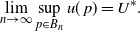
Proof. We begin by giving the idea of the proof. Suppose that the payoff function u is ${\mathcal R}^{\rm DS}$ -integrable. Let $U^*=\sup_{p\in P}u(\,p)$ . Without being precise, the main idea is to construct a sequence of clopen sets $B_1\supseteq B_2\supseteq B_3\supseteq\cdots$ of plays such that the best value of u on $B_n$ converges to $U^*$ :

(5) \begin{equation} \lim_{n\to\infty} \sup_{p\in B_n}u(\,p) = U^*. \label{eqn5} \end{equation}

Let us say that a history h is consistent with $B_n$ if $B_n$ contains a play that starts with h. This means that at h we still have the possibility to stay in $B_n$ .

We then construct a behavior strategy b that behaves as follows. Consider a history h. There are three cases. If h is not consistent with any $B_n$ , then b(h) is arbitrary. If h is consistent with $B_1,\ldots,B_n$ but not with $B_{n+1},B_{n+2},\ldots$ , then b(h) places probability 1 on an action that keeps consistency with $B_n$ . Finally, if h is consistent with every $B_n$ , then b(h) intuitively recommends choosing a natural number n according to a diffuse charge on $({\mathbb{N}}, 2^{{\mathbb{N}}})$ and then playing an action that keeps consistency with $B_n$ . So, the idea of the behavior strategy b is to stay consistent with $B_n$ for as large values of n as possible. It will then follow from (5) that b is $({\mathcal R}^{\rm DS},\psi^{\rm DS})$ -optimal, as desired.

The formal proof consists of four steps.

step 1. In this part of the proof we construct a number of objects:

1. (i) For every $n\in{\mathbb{N}}$ , we construct an ${\mathcal R}^{\rm DS}$ -measurable simple function $u_n$ of the form

   \[u_n(\,p) = \sum_{B\in \mathcal{B}_n} c_B\cdot\mathbb{I}_{B}(\,p), \]
   where $c_B\in\mathbb{R}$ for every $B\in \mathcal{B}_n$ and $\mathcal{B}_n\subseteq {\mathcal R}^{\rm DS}$ is a finite partition of P. Our construction guarantees that the following properties hold for every $n\in{\mathbb{N}}$ : (i.1) $u_n\leq u$ ; (i.2) $\sup_{p\in P}|u_n(\,p)-u(\,p)|\leq \frac{1}{n}$ for every play $p\in P$ ; and (i.3) the partition $\mathcal{B}_{n+1}$ is (weakly) finer than the partition $\mathcal{B}_{n}$ : every set in $\mathcal{B}_{n+1}$ is a subset of a set in $\mathcal{B}_{n}$ .

2. (ii) For every $n\in{\mathbb{N}}$ we identify a set $B_n\in \mathcal{B}_n$ such that (ii.1) for every $n\in{\mathbb{N}}$ , $B_n\supseteq B_{n+1}$ ; (ii.2) $c_{B_n}$ converges to $U^*$ as n tends to infinity.

Construction for (i): The function u is ${\mathcal R}^{\rm DS}$ -integrable. Hence, as discussed in Section 2, for every $n\in{\mathbb{N}}$ there exists an ${\mathcal R}^{\rm DS}$ -measurable simple function $v_n$ such that $\sup_{p\in P}|v_n(\,p)-u(\,p)|\leq \frac{1}{2n}$ for every play $p\in P$ . Let $u_n(\,p)=v_n(\,p)-\frac{1}{2n}$ for every play $p\in P$ . Then, for every $n\in{\mathbb{N}}$ , $u_n$ is an ${\mathcal R}^{\rm DS}$ -measurable simple function such that $u_n\leq u$ and $\sup_{p\in P}|u_n(\,p)-u(\,p)|\leq \frac{1}{n}$ for every play $p\in P$ . So, (i.1) and (i.2) hold. For each $n\in{\mathbb{N}}$ , let $\mathcal{B}_n\subseteq {\mathcal R}^{\rm DS}$ be the partition of the set P of plays corresponding to $u_n$ . By splitting sets in $\mathcal{B}_2$ if necessary, we can achieve that $\mathcal{B}_{2}$ is (weakly) finer than the partition $\mathcal{B}_{1}$ . Next, by splitting sets in $\mathcal{B}_3$ if necessary, we can achieve that $\mathcal{B}_{3}$ is (weakly) finer than the partition $\mathcal{B}_{2}$ . By continuing this way, we can make sure that (i.3) holds as well.

Construction for (ii): For every $n \in {\mathbb{N}}$ let the play $p_n \in P$ be such that $u(\,p_n) \geq U^* - \tfrac{1}{n}$ . Because the partition $\mathcal{B}_1$ is finite, there exists a set $B_1 \in \mathcal{B}_1$ such that the set $\{m \in {\mathbb{N}}: p_m \in B_1\}$ is infinite. Because $\mathcal{B}_2$ is finer than $\mathcal{B}_1$ , there also exists a set $B_2 \in \mathcal{B}_2$ such that $B_2\subseteq B_1$ and the set $\{m \in {\mathbb{N}}: p_m \in B_2\}$ is infinite. Continuing in this way we define $B_n$ for each $n\in {\mathbb{N}}$ , and then (ii.1) holds. Now assume that $p_m\in B_n$ for some $m,n\in{\mathbb{N}}$ . Then, by the choice of the play $p_m$ , by (i.2), and by $p_m\in B_n$ , we have

(6) \begin{equation} U^*-\frac{1}{m} \leq u(\,p_m) \leq u_n(\,p_m) +\frac{1}{n} = c_{B_n}+\frac{1}{n}. \label{eqn6} \end{equation}

As the set $\{m \in {\mathbb{N}}: p_m \in B_n\}$ is infinite, the inequality (6) holds for infinitely many $m\in{\mathbb{N}}$ , and hence

\[U^* \leq c_{B_n}+\frac{1}{n}.\]

This implies that (ii.2) holds as well.

Step 2. In this step we construct a behavior strategy b. First, we need some notation. Take a history $h \in H$ . Let

\begin{align*} N^*_h = \{n \in {\mathbb{N}}: [h]\cap B_n \neq \Oslash\}. \end{align*}

Intuitively, $n\in N^*_h$ means that the history h is consistent with the set $B_n$ in the sense that there is a play in $B_n$ that extends h. More precisely, if $n\in N^*_h$ , then there is a play $p^n_h\in \mathcal{B}_n$ such that $h\prec p^n_h$ , and hence there is an action $a^n_h\in A$ , i.e. the action in $p^n_h$ after h, such that $(h,a^n_h)\prec p^n_h$ . Notice the following properties for any history $h\in H$ :

1. (a) If $m\in N^*_h$ and $n\leq m$ , then $n\in N^*_h$ and $n\in N^*_{(h,a^m_h)}$ . We prove this property.

   Assume $m\in N^*_h$ and $n\leq m$ . Then, by (ii.1), $[h]\cap \mathcal{B}_n\supseteq [h]\cap \mathcal{B}_m\neq \Oslash$ , and hence $n\in N^*_h$ .

   Further, as $m\in N^*_h$ , we have $p^m_h\in [(h,a^m_h)]\cap \mathcal{B}_m$ , which implies that $[(h,a^m_h)]\cap \mathcal{B}_m\neq\oslash$ . Hence, $m\in N^*_{(h,a^m_h)}$ . By the previous part, $n\in N^*_{(h,a^m_h)}$ .

2. (b) We have one of the following three cases: $N^*_h$ is empty, or $N^*_h=\{1,\ldots,m\}$ for some $m\in{\mathbb{N}}$ , or $N^*_h={\mathbb{N}}$ . This follows from property (a).

Now we define a behavior strategy b. Take an arbitrary history $h\in H$ . We need to define the charge $b(h)\in\mathcal{C}(A,2^A)$ . Based on property (b), we distinguish three different cases. If $N^*_h$ is empty, then let b(h) be an arbitrary charge on the action space. If $N^*_h=\{1,\ldots,m\}$ for some $m\in{\mathbb{N}}$ , then define b(h) to be the Dirac charge on $a^m_h$ . That is, for every set $B \subseteq A$ , we have $b(h)(B) =1$ if $a^m_h \in B$ and $b(h)(B)=0$ if $a^m_h \notin B$ . Finally, if $N^*_h={\mathbb{N}}$ , then let $\tau$ be a diffuse charge on $({\mathbb{N}},2^{\mathbb{N}})$ , and define b(h) by for each $A'\subseteq A$ letting

\[b(h)(A') = \tau(\{n\in{\mathbb{N}}:a^n_h\in A'\}).\]

Intuitively, in this final case b(h) recommends choosing a natural number n according to $\tau$ and then playing the action $a^n_h$ . So, in all three cases the idea of the behavior strategy b is to stay consistent with $B_n$ for as large values of n as possible.

Step 3. We show that $\psi^{\rm DS}(b)(B_n)=1$ for every $n \in {\mathbb{N}}$ . Take $n \in {\mathbb{N}}$ . We prove this by applying Lemma 5. Let $Q=B_n$ . We already know that Q is clopen, as $Q=B_n\in\mathcal{B}_n\subseteq{\mathcal R}^{\rm DS}$ . Take a history $h\in H$ , and assume that $Q|_h\neq \Oslash$ . Then there is a play $p\in Q$ such that $p\succ h$ . Thus, $n\in N^*_h\neq \Oslash$ .

In view of property (b), we have two cases. Assume first that $N^*_h=\{1,\ldots,m\}$ for some $m\in{\mathbb{N}}$ . Obviously, $m\geq n$ . By property (a), $n\in N^*_{(h,a^m_h)}$ . Thus, $Q|_{(h,a^m_h)}\neq \Oslash$ . Recall that b(h) is the Dirac charge on $a^m_h$ in this case, so b satisfies the condition of Lemma 5. Assume next that $N^*_h={\mathbb{N}}$ . For every $m\geq n$ , by property (a), $n\in N^*_{(h,a^m_h)}$ and hence $Q|_{(h,a^m_h)}\neq \Oslash$ . As $b(h)(\{a^n_h,a^{n+1}_h,\ldots\}) % = % 1$ , the strategy b satisfies the condition of Lemma 5 in this case as well.

Thus, by Lemma 5, $\psi^{\rm DS}(b)(Q)=1$ , i.e. $\psi^{\rm DS}(b)(B_n)=1$ , as desired.

Step 4. We show that the behavior strategy b is $({\mathcal R}^{\rm DS},\psi^{\rm DS})$ -optimal. By (i.1) and by Step 3, we have for every $n \in {\mathbb{N}}$ that

\[\int_{p \in P} u (\,p) \, \psi^{\rm DS}(b)( {\rm d} p) \geq \int_{p \in P} u_n (\,p) \, \psi^{\rm DS}(b)( {\rm d} p) = c_{B_n}.\]

Hence, by (ii.2),

\[\int_{p \in P} u (\,p) \, \psi^{\rm DS}(b)( {\rm d} p) = U^*.\]

This completes the proof.

6.1. Equivalence from mixed strategies to behavior strategies

We first demonstrate that even if the action space is finite, there is a mixed strategy m that has no $({\mathcal{P}},\psi^{\mathcal{P}})$ -equivalent behavior strategy for any competent algebra ${\mathcal{P}}$ on the set P of plays that contains all singleton plays and any ${\mathcal{P}}$ -specification $\psi^{\mathcal{P}}$ that respects singleton plays.

This mixed strategy m has no $({\mathcal{P}},\psi^{\mathcal{P}})$ -equivalent behavior strategy for any competent algebra ${\mathcal{P}}$ on the set P of plays that contains all singleton plays and any ${\mathcal{P}}$ -specification $\psi^{\mathcal{P}}$ that respects singleton plays. A precise argument follows from the proof of Theorem 6. Here we only provide the intuition.

Let b be a behavior strategy. Also, for every $n\in{\mathbb{N}}$ , let $c^n$ denote the history $(c,\ldots,c)$ of length n, and let $c^\infty$ denote the play only having action c. As the probability under m that the decision maker plays action s in the first T periods is 0 for every $T \in {\mathbb{N}}$ , if $b(c^n)$ does not put probability 1 on action c for some $n\in N$ then b cannot be $({\mathcal{P}},\psi^{\mathcal{P}})$ -equivalent to m. So, assume that $b(c^n)$ puts probability 1 on action c for all $n\in N$ . Then, as the singleton $\{c^\infty\}$ is contained in the algebra ${\mathcal{P}}$ , by (7) we have $\psi(b)(\{c^\infty\})=1$ . Because $m^*(\{c^\infty\})=0$ , also in this case b cannot be $({\mathcal{P}},\psi^{\mathcal{P}})$ -equivalent to m.

The following theorem is based on Example 1.

Proof. Let a and a’ denote two different actions in A. For every $n\in{\mathbb{N}}$ , let $p_n$ denote the play that has action a up to period n and has action a’ from period $n+1$ onwards. The sequence of plays $(\,p_n)_{n\in{\mathbb{N}}}$ converges to the play $p=(a,a,\ldots)$ .

For all $n\in{\mathbb{N}}$ , let $f_n$ denote a pure strategy that induces the play $p_n$ . Let $\tau$ be a diffuse charge on $({\mathbb{N}},2^{\mathbb{N}})$ . Now consider the mixed strategy m that, intuitively, first chooses a natural number $n\in {\mathbb{N}}$ according to $\tau$ and then plays the pure strategy $f_{n}$ . Formally, for every subset F’ of the set F of pure strategies we have

\[m(F') = \tau(\{n\in{\mathbb{N}} \mid f_{n}\in F'\}).\]

Hence, for every $P'\subseteq P$ ,

\[m^*(P') = \tau(\{n\in{\mathbb{N}} \mid p_{n}\in P'\}).\]

We show that the mixed strategy m has no $({\mathcal{P}},\psi^{\mathcal{P}})$ -equivalent behavior strategy. Indeed, take any behavior strategy b. We distinguish two cases.

First, assume that there is a history of the form $h=(a,\ldots,a)\prec p$ such that the charge b(h) places probability less than 1 on action a. We can assume that h is the shortest history with this property. Let Q be the set of all histories of the form (h,x) where $x\in A\setminus \{a\}$ . The set [Q] belongs to the algebra ${\mathcal R}^{\rm f}\subseteq {\mathcal{P}}$ , and

\[\psi^{\mathcal{P}}(b)([Q]) = c^{\rm f}(b)([Q]) = 1-b(h)(a) > 0.\]

This is, however, in contradiction with $m^*([Q])=0$ .

Now assume that for every history of the form $h=(a,\ldots,a)\prec p$ , the charge b(h) places probability 1 on action a. As $\psi^{\mathcal{P}}$ respects singleton plays, $\psi^{\mathcal{P}}(b)(\{p\})=1$ . This contradicts $m^*(\{p\})=0$ .

Thus, the mixed strategy m has no $({\mathcal{P}},\psi^{\mathcal{P}})$ -equivalent behavior strategy.

Theorem 6 applies to several algebras that have been previously considered in the literature. For example, Dubins (Reference Dubins1974) considered the algebra generated by open sets, and Purves and Sudderth (Reference Purves and Sudderth1976) considered the Borel sigma-algebra. Part of the authors’ motivation concerns stating finitely additive generalizations of classical probabilistic limit laws in the usual fashion.

Both the previously mentioned algebras are competent and contain all singletons, and their corresponding specifications respect singleton plays. In the remainder of this subsection we show that Theorem 6 applies to the algebra generated by the open sets and the corresponding specification.

Given a charge $\mu$ on the clopen subsets of P, Dubins (Reference Dubins1974) defined a probability for each open subset of P through inner approximations by clopen sets. That is, if $O\subseteq P$ is open, then he let $\mu'(O)$ be the supremum of $\mu(Z)$ where $Z\subseteq O$ is clopen. His Theorem 2 showed that this mapping $\mu'$ defined on the open sets has a unique extension to a charge on the whole algebra generated by the open sets.

By translating the result of Dubins (Reference Dubins1974), we now define a competent algebra and a specification. For every behavior strategy b and open set $O\subseteq P$ we let

(8) \begin{equation} c^{\rm o}(b)(O) = \sup_{Z\in{\mathcal R}^{\rm DS},Z\subseteq O}\,\psi^{\rm DS}(b)(Z). \label{eqn8} \end{equation}

Let ${\mathcal R}^{\rm o}$ be the algebra generated by the open subsets of P. That is, ${\mathcal R}^{\rm o}$ is the smallest algebra of subsets of P that contains all open sets. By Lemma 3, ${\mathcal R}^{\rm f}\subseteq {\mathcal R}^{\rm DS}\subset {\mathcal R}^{\rm o}$ . So, in particular, ${\mathcal R}^{\rm o}$ is competent.

By the result of Dubins (Reference Dubins1974), for every behavior strategy b there is a unique charge $\psi^{\rm o}(b)$ on the algebra ${\mathcal R}^{\rm o}$ such that, for every open set $O\subseteq P$ ,

(9) \begin{equation} \psi^{\rm o}(b)(O) = c^{\rm o}(b)(O). \label{eqn9} \end{equation}

Observe the following. If $Q\in {\mathcal R}^{\rm f}$ then $Q\in{\mathcal R}^{\rm DS}$ , and hence in view of (9), (8), and (4) we have for every behavior strategy b that

(10) \begin{equation} \psi^{\rm o}(b)(Q) = c^{\rm o}(b)(Q) = \psi^{\rm DS}(b)(Q) = c^{\rm f}(b)(Q). \label{eqn10} \end{equation}

This means that $\psi^{\rm o}$ is an ${\mathcal R}^{\rm o}$ -specification.

Proof. Since each singleton $\{p\}$ , where $p\in P$ , is closed, ${\mathcal R}^{\rm o}$ contains all singleton plays.

We now show that $\psi^{\rm o}$ respects singleton plays. Let b be a behavior strategy and let $p=(a_1,a_2,\ldots)\in P$ . For each $n\in{\mathbb{N}}$ , let $H_n \subset A^n$ denote the set of histories at period n that follow p until period $n-1$ and then deviate from $a_n$ at period n:

\[H_n = \{(a_1,\ldots,a_{n-1},a):a\neq a_{n}\},\]

and let $Q_n=H_1\cup\cdots \cup H_n$ . For each $n\in{\mathbb{N}}$ , we have $Q_n\in {\mathcal R}^{\rm f}$ , and hence, by (10),

\[\psi^{\rm o}(b)(Q_n) = c^{\rm f}(b)(Q_n) = 1-c^{\rm f}(b)([a_1,\ldots,a_n]) = 1-\prod_{k=1}^n {b(a_1,\ldots,a_{k-1})(a_{k})}.\]

Now take any clopen set $Q\subset P\setminus \{p\}$ . It is easy to see that there is $n\in {\mathbb{N}}$ such that $Q\subseteq Q_n$ . Indeed, otherwise p would be a limit point of Q, which is impossible. As $Q_n\subset P\setminus \{p\}$ , we obtain

\[\sup_{Q\in{\mathcal R}^{\rm DS},Q\subseteq P\setminus \{p\}}\psi^{\rm o}(Q) = \sup_{n\in{\mathbb{N}}}\psi^{\rm o}(Q_n) = 1-\prod_{k=1}^\infty {b(a_1,\ldots,a_{k-1})(a_{k})}.\]

Since $P\setminus \{p\}$ is open, by (9) and (8) we have

\[\psi^{\rm o}(P\setminus \{p\}) = 1-\prod_{k=1}^\infty {b(a_1,\ldots,a_{k-1})(a_{k})},\]

implying

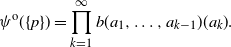\[\psi^{\rm o}(\{p\}) = \prod_{k=1}^\infty {b(a_1,\ldots,a_{k-1})(a_{k})}.\]

Thus, $\psi^{\rm o}(b)$ respects singleton plays.

The next theorem follows from Lemma 6 and Theorem 6.

We emphasize that the specification $\psi^{\rm o}$ defines a charge on ${\mathcal R}^{\rm o}$ for all behavior strategies. Given a specific behavior strategy b, Purves and Sudderth (Reference Purves and Sudderth1976) extended the charge $\psi^{\rm o}(b)$ from the algebra ${\mathcal R}^{\rm o}$ to $\mathcal{A}(b)$ . The algebra $\mathcal{A}(b)$ contains the sets of plays which can be approximated by closed sets from the inside and open sets from the outside in such a way that the $\psi^{\rm o}(b)$ -probability of their difference can be made arbitrarily small (see their Proposition 2.1). Their Theorem 5.1 showed that all elements of the Borel sigma-algebra on P can be approximated this way, so the Borel sigma-algebra is a subset of $\mathcal{A}(b)$ . This means that for every behavior strategy b there is a charge defined on the Borel sigma-algebra which agrees with $\psi^{\rm o}(b)$ on the algebra ${\mathcal R}^{\rm o}$ .

6.2 Existence of an optimal behavior strategy

The following theorem is in contrast with Theorem 5 that we obtained under the approach of Dubins and Savage.

Proof. Take an action $a\in A$ . Let the payoff function u be defined as follows: if the decision maker chooses an action other than a at period n for the first time, then the payoff is $\frac{n}{n+1}$ ; if they choose action a at all periods, then the payoff is 0. More precisely, for every $n\in{\mathbb{N}}$ , let $H_n$ denote the histories of length n of the form $(a,\ldots,a,a')$ , where $a'\in A\setminus \{a\}$ . Then $u(\,p)=\frac{n}{n+1}$ if $p\in [H_n]$ for some $n\in {\mathbb{N}}$ , and $u(a,a,\ldots)=0$ .

We show that u is ${\mathcal{P}}$ -integrable by proving that for every ${\varepsilon}>0$ there exists a ${\mathcal{P}}$ -measurable simple function $u':P\rightarrow \mathbb{R}$ such that $|u(\,p)-u'(\,p)|\leq {\varepsilon}$ for every $p\in P$ . Indeed, take ${\varepsilon}>0$ , and let $m\in {\mathbb{N}}$ such that $m\geq \frac{1-{\varepsilon}}{{\varepsilon}}$ . Consider the partition of P consisting of the following sets:

\[[H_1],\ [H_2],\ \ldots,\ [H_{m-1}],\ \bigcup\limits_{k\geq m} [H_{m}]\setminus \{(a,a,\ldots)\},\ \{(a,a,\ldots)\}.\]

Since each $[H_n]$ belongs to ${\mathcal R}^{\rm f}$ , and since the algebra ${\mathcal{P}}$ is competent and contains all singleton plays (in particular it contains $\{(a,a,\ldots)\}$ ), we can conclude that all these sets belong to ${\mathcal{P}}$ . Define the following function $u':P\rightarrow \mathbb{R}$ . Let $u'(\,p)=u(\,p)=\frac{n}{n+1}$ if $p\in [H_n]$ for some $n\leq m-1$ , let $u'(\,p)=1$ for all $p\in \cup_{k\geq m} [H_{m}]\setminus \{(a,a,\ldots)\}$ , and let $u'(a,a,\ldots)=u(a,a,\ldots)=0$ . It follows that u’ is a ${\mathcal{P}}$ -measurable simple function such that $|u(\,p)-u'(\,p)|\leq {\varepsilon}$ for every $p\in P$ .

It follows similarly to the proof of Theorem 6 that there is no behavior strategy b such that $U(b \mid {\mathcal{P}},\psi^{\mathcal{P}})=1$ . This means that there is no $({\mathcal{P}},\psi^{\mathcal{P}})$ -optimal behavior strategy.