2. Two kinds of surface currents in the thin wall

For the purpose of TMHD modelling, the surface current density $h\boldsymbol{j}$ in the conducting shell ( $h$ is the thickness of the current distribution) can be split into two components: (i) a divergence-free surface current $\boldsymbol{i}$ , and (ii) a current $\propto -\boldsymbol{{\rm\nabla}}{\it\phi}^{S}$ with potentially finite divergence to describe current sharing between the plasma and the wall:

(2.1) $$\begin{eqnarray}\displaystyle h\boldsymbol{j}=\boldsymbol{i}-\bar{{\it\sigma}}\boldsymbol{{\rm\nabla}}{\it\phi}^{S},\quad \boldsymbol{i}\equiv \boldsymbol{{\rm\nabla}}I\times \boldsymbol{n},(\boldsymbol{{\rm\nabla}}\boldsymbol{\cdot }\boldsymbol{i})=0,\bar{{\it\sigma}}\equiv h{\it\sigma}. & & \displaystyle\end{eqnarray}$$

Here, $I$ is the stream function of the divergence-free component and $\boldsymbol{n}$ the unit normal vector to the wall. The $\boldsymbol{i}$ component corresponds to the well-known eddy currents. Following Riccardo et al. (Reference Riccardo, Noll and Walker2000), we refer to the second component $-\bar{{\it\sigma}}\boldsymbol{{\rm\nabla}}{\it\phi}^{S}$ as the source/sink current, or S/S-current. Accordingly, the surface function ${\it\phi}^{S}$ is called the source/sink potential.

The S/S-current in (2.1) is the surface current which originates from the sharing of the electric current between the plasma and the wall. It is determined from the following equation

(2.2) $$\begin{eqnarray}\displaystyle (\boldsymbol{{\rm\nabla}}\boldsymbol{\cdot }(h\boldsymbol{j}))=-(\boldsymbol{{\rm\nabla}}\boldsymbol{\cdot }(\bar{{\it\sigma}}\boldsymbol{{\rm\nabla}}{\it\phi}^{S}))=j_{\bot },\quad j_{\bot }\equiv -(\boldsymbol{j}\boldsymbol{\cdot }\boldsymbol{n})=j_{\bot }^{Hr}+j_{\bot }^{Ev}, & & \displaystyle\end{eqnarray}$$

where $j_{\bot }$ is the density of the current coming from/to the plasma and acting as a galvanic source for the surface currents on the wall. The sign of $j_{\bot }$ is positive for the current from the plasma to the wall, which corresponds to the source. The part $j_{\bot }^{Hr}$ of $j_{\bot }$ can be associated with the Hiro currents, which are excited inductively due to plasma deformation and its contact with the wall. The amplitude of the Hiro currents are not sensitive to the details of the plasma–wall interaction (the instability acts as a current generator). For wall simulations, these currents and their wetting zone can be considered to be given. The TMHD disruption model splits the equation of motion into an equilibrium equation and the plasma advancing equation. The splitting allows disruption simulations on a relatively slow time scale in comparison with the fast time of ideal MHD instabilities (Zakharov & Li Reference Zakharov and Li2015). In a thin HSoL approximation (the ${\it\delta}$ -functional Hiro currents) the equilibrium equation determines the shape of the contact zone, the contour of the entrance and the amplitude of the Hiro currents along this contour. A more realistic model should include the finite thickness of HSoL, an additional item of edge physics which determines the structure of HSoL.

Another, $j_{\bot }^{Ev}$ , part of $j_{\bot }$ is associated with the Evans currents in the conventional SoL (Zakharov et al. Reference Zakharov, Galkin and Gerasimov2012; Zakharov & Li Reference Zakharov and Li2015) created by the plasma particles released from the shrinking plasma core when the plasma touches the material surface. The toroidal loop voltage drives the current in this SoL along the open field lines. This current is ‘source’ limited by the rate of the electric charge release $e\,\text{d}N/\text{d}t$ , where $N$ is the number of particles in the plasma core. Unlike the Hiro currents, which are an inductive effect of the instability, the Evans currents represent a side ‘resistive’ effect, which depends on plasma–wall interactions. Being source limited, these currents are small relative to the Hiro currents and do not affect the disruption dynamics. However they can be measured and should be simulated, thus providing information regarding plasma–wall interactions during disruptions.

Both Hiro and Evans currents from the SoL enter the wall surface in the vicinity of the contour of the wetting zone, whose geometry is determined by the plasma dynamics. The amplitude and direction of the Hiro currents is determined dynamically by the plasma deformation and flux conservation. The waveform of the total Evans current $I^{Ev}(t)$ is considered as input. In a thin HSoL and SoL approximation, which is the simplest reasonable model, the current density $j_{\bot }$ can be considered as ${\it\delta}$ -functional along the wetting-zone contour. In this paper, for demonstration of the capabilities of the numerical codes, $j_{\bot }$ -profiles distributed over the wetting zone are used.

In terms of components of the surface current, Faraday’s law can be written as

(2.3) $$\begin{eqnarray}\displaystyle -\frac{\partial \boldsymbol{A}}{\partial t}-\boldsymbol{{\rm\nabla}}{\it\phi}^{E}=\bar{{\it\eta}}(\boldsymbol{{\rm\nabla}}I\times \boldsymbol{n})-\boldsymbol{{\rm\nabla}}{\it\phi}^{S},\quad \bar{{\it\eta}}\equiv \frac{1}{\bar{{\it\sigma}}}. & & \displaystyle\end{eqnarray}$$

Here, $\boldsymbol{A}$ is the vector potential of the magnetic field and ${\it\phi}^{E}$ is the electric potential. The effective resistance $\bar{{\it\eta}}$ is introduced for convenience.

The normal component of the curl of this equation gives the equation for the stream function $I$ (Tseitlin Reference Tseitlin1970; Chance Reference Chance1997; Chance et al. Reference Chance, Chu, Okabayashi and Turnbull2002; Chu et al. Reference Chu, Chance, Glasser and Okabayashi2003; Pustovitov Reference Pustovitov2008; Strumberger et al. Reference Strumberger, Merkel, Sempf and Günter2008; Atanasiu, Moraru & Zakharov Reference Atanasiu, Moraru and Zakharov2009; In et al. Reference In2009; Atanasiu & Zakharov Reference Atanasiu and Zakharov2013)

(2.4) $$\begin{eqnarray}\displaystyle (\boldsymbol{{\rm\nabla}}\boldsymbol{\cdot }(\bar{{\it\eta}}\boldsymbol{{\rm\nabla}}I))=\frac{\partial B_{\bot }}{\partial t}=\frac{\partial (B_{\bot }^{pl}+B_{\bot }^{coil}+B_{\bot }^{I}+B_{\bot }^{S})}{\partial t}. & & \displaystyle\end{eqnarray}$$

On the right-hand side, the normal component of the magnetic field is represented by separate contributions from the plasma $B_{\bot }^{pl}$ , external coils $B_{\bot }^{coil}$ and from two components of the surface current, $B_{\bot }^{I}$ and $B_{\bot }^{S}$ .

Two equations (2.2), (2.4) describe the current distribution in the thin wall given the sources $j_{\bot },B_{\bot }^{pl},B^{coil}$ specified as functions of space and time. In addition to (2.2), (2.4), the expression for the magnetic field from the surface current (e.g. Biot–Savart formulas), has to be specified in order to close the system of equations. The important property of this system of equations is the independence of (2.2) for ${\it\phi}^{S}$ from (2.4). Solved independently, it contributes via the term $\partial B^{S}/\partial t$ to the right-hand side of (2.4).

Equations (2.2), (2.4) can be solved using the finite difference method, e.g. as in (Atanasiu & Zakharov Reference Atanasiu and Zakharov2013) for simulation of the thin-wall response to the perturbations from a rotating kink mode. In this paper, the implementation of a more universal method is described.

3. Triangle model for two kinds of surface current in the wall

The triangle electromagnetic representation of the thin wall is based on the following expressions for the vector potential $\boldsymbol{A}$ and magnetic field $\boldsymbol{B}$ of a uniform surface current $\boldsymbol{i}=\text{const.}$ inside the triangle

(3.1) $$\begin{eqnarray}\displaystyle & \displaystyle \boldsymbol{A}(\boldsymbol{r})=h\boldsymbol{j}{\it\varphi}(\boldsymbol{r})=[(\boldsymbol{{\rm\nabla}}I\times \boldsymbol{n})-\bar{{\it\sigma}}\boldsymbol{{\rm\nabla}}{\it\phi}^{S}]{\it\varphi}(\boldsymbol{r}),\quad {\it\varphi}(\boldsymbol{r})\equiv \int \frac{\text{d}S^{\prime }}{X}, & \displaystyle\end{eqnarray}$$

(3.2) $$\begin{eqnarray}\displaystyle & \displaystyle \boldsymbol{B}(\boldsymbol{r})=(h\boldsymbol{j}\times \boldsymbol{e})=\{[(\boldsymbol{{\rm\nabla}}I\times \boldsymbol{n})-\bar{{\it\sigma}}\boldsymbol{{\rm\nabla}}{\it\phi}^{S}]\times \boldsymbol{e}\},\quad \boldsymbol{e}(\boldsymbol{r})\equiv \int \frac{\boldsymbol{X}}{X^{3}}\,\text{d}S^{\prime }, & \displaystyle\end{eqnarray}$$

(3.3a,b ) $$\begin{eqnarray}\displaystyle \boldsymbol{X}\equiv \boldsymbol{r}-\boldsymbol{r}^{\prime },\quad X\equiv |\boldsymbol{r}-\boldsymbol{r}^{\prime }|, & & \displaystyle\end{eqnarray}$$

where ${\it\varphi}$ is the electric potential of a triangle with a uniform unit charge, $\boldsymbol{e}$ is its electric field, $\boldsymbol{r},\boldsymbol{r}^{\prime }$ are the coordinates of the observation and the source points and the integrals are taken over the surface of the triangle. Both ${\it\varphi}$ and $\boldsymbol{e}$ have analytical expressions in terms of elementary functions.

In 2008, the triangle based electrodynamic model of the thin wall was implemented into the numerical Shell simulation code (SHL), mentioned in (Zakharov et al. Reference Zakharov, Galkin and Gerasimov2012) and used for simulations of eddy currents in the lithium tokamak experiment (LTX) (Berzak et al. Reference Berzak, Menard, Majeski, Lundberg, Granstedt, Jacobson, Kaita, Kozub and Zakharov2012). Earlier, the triangle based wall model was implemented into the STARWALL code of Merkel (Merkel, Nührenberg & Strumberger Reference Merkel, Nührenberg and Strumberger2004; Merkel & Sempf Reference Merkel and Sempf2006; Strumberger et al. Reference Strumberger, Merkel, Sempf and Günter2008; Merkel & Strumberger Reference Merkel and Strumberger2015) for resistive wall-mode studies.

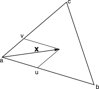
Inside a triangle with vertices a, b, c (figure 1) the edges and the local vector of an arbitrary point are defined as

(3.4a−d ) $$\begin{eqnarray}\displaystyle \boldsymbol{x}\equiv \boldsymbol{r}-\boldsymbol{r}_{a},\quad \boldsymbol{r}_{ba}\equiv \boldsymbol{r}_{b}-\boldsymbol{r}_{a},\quad \boldsymbol{r}_{cb}\equiv \boldsymbol{r}_{c}-\boldsymbol{r}_{b},\quad \boldsymbol{r}_{ac}\equiv \boldsymbol{r}_{a}-\boldsymbol{r}_{c}. & & \displaystyle\end{eqnarray}$$

For calculation of the finite elements, new coordinates $u,v$ , with the origin in the vertex $a$ , are introduced by

(3.5a−d ) $$\begin{eqnarray}\displaystyle \boldsymbol{x}(u,v)\equiv \boldsymbol{r}_{ba}u-\boldsymbol{r}_{ac}v,\quad \boldsymbol{x}(0,0)=0,\quad \boldsymbol{x}(1,0)=\boldsymbol{r}_{ba},\quad \boldsymbol{x}(0,1)=-\boldsymbol{r}_{ac}.\quad & & \displaystyle\end{eqnarray}$$

Figure 1.

Elementary triangle.

The metric tensor is determined by an element of length $\text{d}l$

(3.6a,b ) $$\begin{eqnarray}\displaystyle \text{d}\boldsymbol{x}(u,v)=\boldsymbol{r}_{ba}\,\text{d}u-\boldsymbol{r}_{ac}\,\text{d}v,\quad \text{d}l^{2}=g_{uu}\,\text{d}u^{2}+2g_{uv}\,\text{d}u\,\text{d}v+g_{vv}\,\text{d}v^{2}, & & \displaystyle\end{eqnarray}$$

(3.7a−c ) $$\begin{eqnarray}\displaystyle g_{uu}=|\boldsymbol{r}_{ba}|^{2},\quad g_{uv}=-(\boldsymbol{r}_{ba}\boldsymbol{\cdot }\boldsymbol{r}_{ac}),\quad g_{vv}=|\boldsymbol{r}_{ac}|^{2}. & & \displaystyle\end{eqnarray}$$

Its Jacobian $D$ is given by

(3.8a,b ) $$\begin{eqnarray}\displaystyle D^{2}=g_{uu}g_{vv}-g_{uv}^{2}=|\boldsymbol{r}_{ba}|^{2}|\boldsymbol{r}_{ac}|^{2}-(\boldsymbol{r}_{ba}\boldsymbol{\cdot }\boldsymbol{r}_{ac})^{2},\quad D=|(\boldsymbol{r}_{ba}\times \boldsymbol{r}_{ac})| & & \displaystyle\end{eqnarray}$$

and is equal to the doubled surface area of the triangle $D=2S$

(3.9a,b ) $$\begin{eqnarray}\displaystyle 2S=|(\boldsymbol{r}_{ba}\times \boldsymbol{r}_{ac})|,\quad \boldsymbol{n}\equiv \frac{(\boldsymbol{r}_{ac}\times \boldsymbol{r}_{ba})}{2S}. & & \displaystyle\end{eqnarray}$$

The gradients of $u,v$ are given by

(3.10a,b ) $$\begin{eqnarray}\displaystyle \boldsymbol{{\rm\nabla}}u=\frac{(\boldsymbol{n}\times \boldsymbol{r}_{ac})}{(\boldsymbol{n}\boldsymbol{\cdot }(\boldsymbol{r}_{ac}\times \boldsymbol{r}_{ba}))}=\frac{(\boldsymbol{n}\times \boldsymbol{r}_{ac})}{D},\quad \boldsymbol{{\rm\nabla}}v=\frac{(\boldsymbol{n}\times \boldsymbol{r}_{ba})}{(\boldsymbol{n}\boldsymbol{\cdot }(\boldsymbol{r}_{ac}\times \boldsymbol{r}_{ba}))}=\frac{(\boldsymbol{n}\times \boldsymbol{r}_{ba})}{D}.\qquad & & \displaystyle\end{eqnarray}$$

The plane functions $I,{\it\phi}^{S}$ inside the triangle are defined by their values $I_{a}$ , $I_{b}$ , $I_{c}$ , ${\it\phi}_{a}^{S}$ , ${\it\phi}_{b}^{S}$ and ${\it\phi}_{c}^{S}$ at the vertices as linear functions of $u,v$

(3.11a,b ) $$\begin{eqnarray}\displaystyle I=I_{a}+(I_{b}-I_{a})u+(I_{c}-I_{a})v,\quad {\it\phi}^{S}={\it\phi}_{a}^{S}+({\it\phi}_{b}^{S}-{\it\phi}_{a}^{S})u+({\it\phi}_{c}^{S}-{\it\phi}_{a}^{S})v. & & \displaystyle\end{eqnarray}$$

The gradient $\boldsymbol{{\rm\nabla}}I$ is given by

(3.12) $$\begin{eqnarray}\displaystyle \boldsymbol{{\rm\nabla}}I=(I_{b}-I_{a})\boldsymbol{{\rm\nabla}}u+(I_{c}-I_{a})\boldsymbol{{\rm\nabla}}v=\left(\frac{I_{a}\boldsymbol{r}_{cb}+I_{b}\boldsymbol{r}_{ac}+I_{c}\boldsymbol{r}_{ba}}{2S}\times \boldsymbol{n}\right), & & \displaystyle\end{eqnarray}$$

where the normal unit vector $\boldsymbol{n}$ is defined in terms of the vector product of the triangle edge vectors. A similar relation is valid for $\boldsymbol{{\rm\nabla}}{\it\phi}^{S}$ .

Now, the total current density inside the triangle, containing both divergence-free and source/sink components, is given by

(3.13) $$\begin{eqnarray}\displaystyle h\boldsymbol{j}=\frac{I_{a}\boldsymbol{r}_{cb}+I_{b}\boldsymbol{r}_{ac}+I_{c}\boldsymbol{r}_{ba}}{2S}+\bar{{\it\sigma}}\left(\frac{{\it\phi}_{a}^{S}\boldsymbol{r}_{cb}+{\it\phi}_{b}^{S}\boldsymbol{r}_{ac}+{\it\phi}_{c}^{S}\boldsymbol{r}_{ba}}{2S}\times \boldsymbol{n}\right). & & \displaystyle\end{eqnarray}$$

4. Energy principle for the thin wall

Equation (2.2) for ${\it\phi}^{S}$ , which determines the current in the wall due to current sharing with the plasma, can be obtained by minimizing the functional $W^{S}$

(4.1) $$\begin{eqnarray}\displaystyle W^{S}=\int \left\{\frac{\bar{{\it\sigma}}(\boldsymbol{{\rm\nabla}}{\it\phi}^{S})^{2}}{2}-j_{\bot }{\it\phi}^{S}\right\}\,\text{d}S-\frac{1}{2}\oint {\it\phi}^{S}\bar{{\it\sigma}}[(\boldsymbol{n}\times \boldsymbol{{\rm\nabla}}{\it\phi}^{S})\boldsymbol{\cdot }\text{d}\boldsymbol{l}]. & & \displaystyle\end{eqnarray}$$

Here, the surface integral $\text{d}S$ is taken along the wall surface, while the contour integral $\text{d}\boldsymbol{l}$ is taken along the edges of the conducting surfaces with the integrand representing the surface current normal to the edges. The contour integral takes into account the external voltage applied to the edges of the wall components and vanishes when there is no source/sink of the current through the edges of the wall surface, as happens in typical cases.

For the divergence-free part of the surface current, the energy principle can be obtained by multiplying the Faraday law equation (2.3) by $\boldsymbol{i}$

(4.2) $$\begin{eqnarray}\displaystyle -\boldsymbol{i}\frac{\partial \boldsymbol{A}}{\partial t}-\boldsymbol{i}\boldsymbol{{\rm\nabla}}({\it\phi}^{E}-{\it\phi}^{S})=\bar{{\it\eta}}|\boldsymbol{i}|^{2} & & \displaystyle\end{eqnarray}$$

and integrating it over the wall surface.

(4.3) $$\begin{eqnarray}\displaystyle -\int \boldsymbol{i}\frac{\partial \boldsymbol{A}}{\partial t}\,\text{d}S+\oint ({\it\phi}^{E}-{\it\phi}^{S})[\boldsymbol{i}\boldsymbol{\cdot }(\boldsymbol{n}\times \text{d}\boldsymbol{l}))=\int \bar{{\it\eta}}|\boldsymbol{i}|^{2}\,\text{d}S. & & \displaystyle\end{eqnarray}$$

The vector potential consists of the following components

(4.4a,b ) $$\begin{eqnarray}\displaystyle \boldsymbol{A}\equiv \boldsymbol{A}^{I}+\boldsymbol{A}^{ext},\quad \boldsymbol{A}^{ext}\equiv \boldsymbol{A}^{pl}+\boldsymbol{A}^{coil}+\boldsymbol{A}^{S}. & & \displaystyle\end{eqnarray}$$

Here $\boldsymbol{A}^{I}$ is the self-field of the current $\boldsymbol{i}$ , while $\boldsymbol{A}^{ext}$ is generated by the plasma $\boldsymbol{A}^{pl}$ , external coils $\boldsymbol{A}^{coil}$ and $\boldsymbol{A}^{S}$ is created by the source/sink current $-\bar{{\it\sigma}}\boldsymbol{{\rm\nabla}}{\it\phi}^{S}$ .

Equation (2.3) for the divergence-free part of the surface current $\boldsymbol{i}=(\boldsymbol{{\rm\nabla}}I\times \boldsymbol{n})$ can be obtained from the following energy functional

(4.5) $$\begin{eqnarray}\displaystyle W^{I}\equiv \frac{1}{2}\int \left\{\frac{\partial (\boldsymbol{i}\boldsymbol{\cdot }\boldsymbol{A}^{I})}{\partial t}+\bar{{\it\eta}}|\boldsymbol{{\rm\nabla}}I|^{2}+2\left(\boldsymbol{i}\boldsymbol{\cdot }\frac{\partial \boldsymbol{A}^{ext}}{\partial t}\right)\right\}\text{d}S-\oint ({\it\phi}^{E}-{\it\phi}^{S})\frac{\partial I}{\partial l}\,\text{d}l. & & \displaystyle\end{eqnarray}$$

The first inductive term in the surface integral represents the change of magnetic energy of the current $\boldsymbol{i}$ , which in the triangle wall model is given by (3.13). Its vector potential $\boldsymbol{A}^{I}$ (3.1) can be expressed in terms of $I$ using explicit formulas for the triangle representation of the wall. The second term describes resistive losses and the third represents the excitation of the current by other sources. If the time derivative is replaced by the growth rate ${\it\gamma}$ , functional (4.5) is reduced to the STARWALL form of the fuctional (Merkel & Sempf Reference Merkel and Sempf2006).

In derivation of (4.5), the term with the time derivative is written in the self-conjugated form by using the equality

(4.6) $$\begin{eqnarray}\displaystyle \left(\frac{\partial \boldsymbol{i}}{\partial t}\boldsymbol{\cdot }\boldsymbol{A}^{I}\right)=\left[\boldsymbol{{\rm\nabla}}\boldsymbol{\cdot }\left(\frac{\partial \boldsymbol{B}^{I}}{\partial t}\times \boldsymbol{A}^{I}\right)\right]+\left[\boldsymbol{{\rm\nabla}}\boldsymbol{\cdot }\left(\frac{\partial \boldsymbol{A}^{I}}{\partial t}\times \boldsymbol{B}^{I}\right)\right]+\left(\frac{\partial \boldsymbol{A}^{I}}{\partial t}\boldsymbol{\cdot }\boldsymbol{i}\right). & & \displaystyle\end{eqnarray}$$

After integration over the entire space, the first two terms on the right-hand side vanish, while for the terms containing $\boldsymbol{i}$ , the volume integral is reduced to the integration over the wall surface, giving

(4.7) $$\begin{eqnarray}\displaystyle \int \!\left(\boldsymbol{i}\boldsymbol{\cdot }\frac{\partial \boldsymbol{A}^{I}}{\partial t}\right)\,\text{d}S=\int \!\left(\frac{\partial \boldsymbol{i}}{\partial t}\boldsymbol{\cdot }\boldsymbol{A}^{I}\right)\,\text{d}S=\frac{1}{2}\frac{\partial }{\partial t}\int (\boldsymbol{i}\boldsymbol{\cdot }\boldsymbol{A}^{I})\,\text{d}S. & & \displaystyle\end{eqnarray}$$

Two energy functionals (4.1) for ${\it\phi}^{S}$ and (4.5) for $I$ are suitable for implementation into the numerical codes and constitute the electromagnetic wall model for the WTKM and WTVM.

5. Matrix circuit equations for triangle wall representation

The substitution of $I,{\it\phi}^{S}$ as a set of plane functions inside triangles (3.12) is straightforward and leads to the finite element representation of $W^{I},W^{S}$ as quadratic forms for the unknowns $I,{\it\phi}^{S}$ at each vertex.

A similar linear representation (3.12) can be chosen for $j_{\bot },\bar{{\it\sigma}}$ and $\bar{{\it\eta}}$

(5.1) $$\begin{eqnarray}\displaystyle & \displaystyle j_{\bot }=j_{a}+(j_{b}-j_{a})u+(j_{c}-j_{a})v, & \displaystyle\end{eqnarray}$$

(5.2) $$\begin{eqnarray}\displaystyle & \displaystyle \bar{{\it\sigma}}=\bar{{\it\sigma}}_{a}+(\bar{{\it\sigma}}_{b}-\bar{{\it\sigma}}_{a})u+(\bar{{\it\sigma}}_{c}-\bar{{\it\sigma}}_{a})v, & \displaystyle\end{eqnarray}$$

(5.3) $$\begin{eqnarray}\displaystyle & \displaystyle \bar{{\it\eta}}=\bar{{\it\eta}}_{a}+(\bar{{\it\eta}}_{b}-\bar{{\it\eta}}_{a})u+(\bar{{\it\eta}}_{c}-\bar{{\it\eta}}_{a})v. & \displaystyle\end{eqnarray}$$

Now, the elementary integrals entering the energy principle (4.1) with these representations of ${\it\phi}^{S},j_{\bot },\bar{{\it\sigma}}$ , can be calculated explicitly as

(5.4a,b ) $$\begin{eqnarray}\displaystyle J_{u}\equiv \frac{1}{S}\int u\,\text{d}S=\frac{2}{D}\int _{0}^{1}u\,\text{d}u\int _{0}^{1-u}D\,\text{d}v=\frac{1}{3},\quad J_{v}\equiv \frac{1}{S}\int v\,\text{d}S=\frac{1}{3}, & & \displaystyle\end{eqnarray}$$

(5.5a−c ) $$\begin{eqnarray}\displaystyle J_{uu}\equiv \frac{1}{S}\int u^{2}\,\text{d}S=\frac{1}{6},\quad J_{vv}\equiv \frac{1}{S}\int v^{2}\,\text{d}S=\frac{1}{6},\quad J_{uv}\equiv \frac{1}{S}\int uv\,\text{d}S=\frac{1}{12}.\quad & & \displaystyle\end{eqnarray}$$

As a result, the energy functional $W^{S}$ can be reduced to the following matrix form

(5.6) $$\begin{eqnarray}\displaystyle W^{S} & \hspace{-2.0pt}=\hspace{-2.0pt} & \displaystyle \mathop{\sum }_{i}\left\{\frac{\bar{{\it\sigma}}_{a}+\bar{{\it\sigma}}_{b}+\bar{{\it\sigma}}_{c}}{3}\frac{({\it\phi}_{a}^{S}\boldsymbol{r}_{cb}+{\it\phi}_{b}^{S}\boldsymbol{r}_{ac}+{\it\phi}_{c}^{S}\boldsymbol{r}_{ba})_{i}^{2}}{8S_{i}}\right.\nonumber\\ \displaystyle & & \displaystyle -\,\left.S_{i}\left.\frac{{\it\phi}_{a}^{S}(2j_{a}+j_{b}+j_{c})+{\it\phi}_{b}^{S}(j_{a}+2j_{b}+j_{c})+{\it\phi}_{c}^{S}(j_{a}+j_{b}+2j_{c})}{12}\right|_{i}\right\},\end{eqnarray}$$

where summation is performed over all triangles. We drop the contour integral term, which is zero for most of plasma dynamics problems.

In the energy functional $W^{I}$ , the vector potential $\boldsymbol{A}^{I}$ is generated by the surface currents from the entire wall

(5.7a,b ) $$\begin{eqnarray}\displaystyle \boldsymbol{A}^{I}(\boldsymbol{r})\equiv \mathop{\sum }_{j}\boldsymbol{i}_{j}{\it\varphi}_{j}(\boldsymbol{r}),\quad \frac{\partial \boldsymbol{A}^{I}(\boldsymbol{r})}{\partial t}=\mathop{\sum }_{j}\frac{({\dot{I}}_{a}\boldsymbol{r}_{cb}+{\dot{I}}_{b}\boldsymbol{r}_{ac}+{\dot{I}}_{c}\boldsymbol{r}_{ba})_{j}}{2S_{j}}{\it\varphi}_{j}(\boldsymbol{r}), & & \displaystyle\end{eqnarray}$$

where the dot stands for the time derivative ${\dot{I}}=\text{d}I/\text{d}t$ . In the energy integral, each $j$ -term in this sum should be integrated over each $i$ -triangle of the wall. The following notation is introduced for the elementary integrals representing the mutual capacitance of two triangles

(5.8) $$\begin{eqnarray}\displaystyle C_{ij}=C_{ji}\equiv \int \text{d}S_{i}\int \frac{\text{d}S_{j}}{|\boldsymbol{r}_{i}-\boldsymbol{r}_{j}|}. & & \displaystyle\end{eqnarray}$$

These have to be evaluated numerically. Other terms in $W^{I}$ can be expressed in the same way as the $W^{S}$ functional.

As a result, $W^{I}$ acquires the following quadratic form representation

(5.9) $$\begin{eqnarray}\displaystyle W^{I} & = & \displaystyle \frac{\text{d}}{\text{d}t}\left\{\mathop{\sum }_{ij}C_{ij}\frac{[(I_{a}\boldsymbol{r}_{cb}+I_{b}\boldsymbol{r}_{ac}+I_{c}\boldsymbol{r}_{ba})_{i}\boldsymbol{\cdot }(I_{a}\boldsymbol{r}_{cb}+I_{b}\boldsymbol{r}_{ac}+I_{c}\boldsymbol{r}_{ba})_{j}]}{8S_{i}S_{j}}\right\}\nonumber\\ \displaystyle & & \displaystyle +\,\mathop{\sum }_{i}\left\{S_{i}\langle \bar{{\it\eta}}\rangle _{i}\cdot \frac{g_{uu}(I_{b}-I_{a})^{2}+2g_{uv}(I_{b}-I_{a})(I_{c}-I_{a})+g_{vv}(I_{c}-I_{a})^{2}}{2}\right\}\nonumber\\ \displaystyle & & \displaystyle +\,\mathop{\sum }_{i}\left\{\frac{[(I_{a}\boldsymbol{r}_{cb}+I_{b}\boldsymbol{r}_{ac}+I_{c}\boldsymbol{r}_{ba})_{i}\boldsymbol{\cdot }\langle \dot{\boldsymbol{A}}^{ext}\rangle _{i}]}{2S_{i}}\right\},\end{eqnarray}$$

with

(5.10a,b ) $$\begin{eqnarray}\displaystyle \langle \bar{{\it\eta}}\rangle _{i}\equiv \frac{\bar{{\it\eta}}_{a}+\bar{{\it\eta}}_{b}+\bar{{\it\eta}}_{c}}{3},\quad \langle \dot{\boldsymbol{A}}^{ext}\rangle _{i}\equiv \frac{\dot{\boldsymbol{A}}_{a}^{ext}+\dot{\boldsymbol{A}}_{b}^{ext}+\dot{\boldsymbol{A}}_{c}^{ext}}{3}. & & \displaystyle\end{eqnarray}$$

Here, the dot at $\dot{\boldsymbol{A}}^{ext}$ stands for the time derivative.

The minimization of quadratic forms (5.6), (5.9) leads to linear systems of equations with symmetric positively defined matrices which can be solved using Cholesky decomposition.

6. Simulations of source/sink currents using SSC code

In accordance with the two types of wall currents, two numerical codes are presented. The SHL implements the matrix equations resulting from $W^{I}$  (5.9), and solves them with given right-hand side $\dot{\boldsymbol{A}}^{ext}$ in (5.9). The SSC complements the SHL by calculation of the S/S-currents in the wall, with given right-hand side $j_{\bot }$ in (5.6).

The wall in both codes is represented as a structure of surfaces. At this moment, by definition there is no electric current sharing between different surfaces across the gaps or along the third dimension (such as grounding). In future, the electric connection between surfaces can be implemented as another $j_{\bot }$ effect.

Each surface consists of a number of vertices and triangles and can contain a single closed edge and potentially multiple holes. The $I$ and ${\it\phi}^{S}$ functions on different surfaces are independent, with $I=0$ along the edges, or at a single point if edges are absent (as for a toroidal shell). Along the edges of the holes $I=\text{const.}$ with values determined by equations. Similarly, the function ${\it\phi}^{S}$ is specified at one of the vertices.

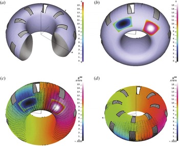
Figure 2 shows an example of calculations of the source/sink currents on a toroidal shell with set vertical and horizontal holes (figure 2 a). In this example, the wall surface does not contain an edge.

Two areas with localized sources (red) and sinks (blue) are prescribed, as shown in figure 2(b) and the wall conductivity $\bar{{\it\sigma}}$ is assumed to be constant and equal to 1 for simplicity. The distribution of the solution $\bar{{\it\sigma}}{\it\phi}^{S}$ of (2.2) over the wall surface (outside the source/sink area) is shown in figure 2(c,d). The colour reflects amplitude in accordance with the colour scale at the right side of each panel. Short straight lines indicate the vectors of the current density $-\bar{{\it\sigma}}\boldsymbol{{\rm\nabla}}{\it\phi}^{S}$ , with the length proportional to its local amplitude, with a dot at the beginning of the vector. The surface currents are concentrated predominantly between source and sink.

Figure 2.

SSC simulations of source/sink currents on a toroidal shell with holes and localized wetting zones. (a) Toroidal thin wall with holes. (b) Wetting zones with distributed $j_{\bot }$ . (c) View to the bottom of the wall on distribution of the solution ${\it\phi}^{S}$ .(d) View to the top where the S/S-currents are small. White and black ends of the colour map correspond to positive and negative values, respectively.

7. Verification of SSC with an analytical solution

The accuracy of the SSC code was checked against the following analytical example. For simplicity, we consider $\bar{{\it\sigma}}=1$ and a toroidal shell, which is shown in figure 3 and defined in Cartesian coordinates $x,y,z$ by

(7.1a−c ) $$\begin{eqnarray}\displaystyle x=(R-a\cos {\it\omega})\cos {\it\varphi},\quad y=(R-a\cos {\it\omega})\sin {\it\varphi},\quad z=a\sin {\it\omega}, & & \displaystyle\end{eqnarray}$$

where ${\it\varphi},{\it\omega}$ are poloidal and toroidal angles and $R,a$ are the major and minor radii. The poloidal and toroidal cuts are defined by

(7.2a,b ) $$\begin{eqnarray}\displaystyle {\it\varphi}_{0}={\it\epsilon}\leqslant {\it\varphi}\leqslant 2{\rm\pi}-{\it\epsilon}={\it\varphi}_{3},\quad {\it\omega}_{0}={\it\epsilon}\leqslant {\it\omega}\leqslant 2{\rm\pi}-{\it\epsilon}={\it\omega}_{3},\quad {\it\epsilon}=0.01, & & \displaystyle\end{eqnarray}$$

The hole area is symmetric with respect to the point ${\it\varphi}={\rm\pi},{\it\omega}={\rm\pi}$ and is specified by

(7.3a−d ) $$\begin{eqnarray}\displaystyle u\equiv {\it\varphi}-{\rm\pi},\quad v\equiv {\it\omega}-{\rm\pi},\quad |u|\leqslant u_{0}=\frac{{\rm\pi}}{4},\quad |v|\leqslant v_{0}=\frac{{\rm\pi}}{4}. & & \displaystyle\end{eqnarray}$$

Figure 3.

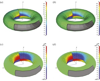
High-resolution model ( $64\times 64\times 4$ triangles) of a wall (the major/minor radii are $3/1$ ). (a) a wall with poloidal and toroidal cuts and a hole in the low field side surface. (b) Colour image of the input $j_{\bot }$ . (c) Colour image of the analytical ${\it\phi}^{S}$ . Straight lines show the direction of the current density with a point labelling the beginning of the vector. (d) The same based on numerical solution. The value of the relative inaccuracy is 0.001.

Figure 4.

(a) Low-resolution triangle model of a wall (the major/minor radii are $3/1$ ). (b) Colour image of the input $j_{\bot }$ . (c) Colour image of the analytical ${\it\phi}^{S}$ . Straight lines show the direction of the current density with a point labelling the beginning of the vector. (d) The same based on numerical solution. The value of the relative inaccuracy is 0.015.

The analytical solution is chosen in the form

(7.4) $$\begin{eqnarray}\displaystyle {\it\phi}^{S}=\int _{0}^{u}G_{u}(u)\,\text{d}u\cdot \int _{0}^{v}G_{v}(v)\,\text{d}v & & \displaystyle\end{eqnarray}$$

with

(7.5) $$\begin{eqnarray}\displaystyle \left.\begin{array}{@{}c@{}}G_{u}(u_{0})=G_{u}(-u_{0})=G_{u}(u_{1})=G_{u}(-u_{1})\\ =G_{v}(v_{0})=G_{v}(-v_{0})=G_{v}(v_{1})=G_{v}(-v_{1})=0,\\ u_{1}=v_{1}={\rm\pi}-{\it\epsilon}\end{array}\right\} & & \displaystyle\end{eqnarray}$$

to satisfy the absence of the current flow through the edges of the shell. One specific choice is given by

(7.6a,b ) $$\begin{eqnarray}\displaystyle G_{u}(u)=(u^{2}-u_{0}^{2})(u^{2}-u_{1}^{2}),\quad G_{v}(v)=(v^{2}-v_{0}^{2})(v^{2}-v_{1}^{2}). & & \displaystyle\end{eqnarray}$$

The source term $j_{\bot }$ for the SSC code can be calculated in a straightforward way with the following relation

(7.7) $$\begin{eqnarray}\displaystyle j_{\bot }=-{\rm\Delta}{\it\phi}^{S}=-\frac{1}{a(R-a\cos {\it\omega})}\left[\frac{a}{R-a\cos {\it\omega}}\frac{\partial ^{2}{\it\phi}^{S}}{\partial {\it\varphi}^{2}}+\frac{\partial }{\partial {\it\omega}}\left(\frac{R-a\cos {\it\omega}}{a}\frac{\partial {\it\phi}^{S}}{\partial {\it\omega}}\right)\right] & & \displaystyle\end{eqnarray}$$

and is shown in figure 3(b).

Figure 3(c,d) illustrate the comparison of the analytical and numerical solutions for different triangularizations of a toroidal shell. A high resolution mesh ( $64\times 64\times 4$ triangles) on the wall surface was used in figure 3(d), providing a relative accuracy of 0.001 (defined as the ratio of maximum deviation of the numerical solution from the exact solution to its maximum value).

Figure 4 represents the same calculations with a rough ( $16\times 15\times 4$ ) resolution, which provide a relative accuracy of 0.015. This is 0.003 for a grid with a mesh $32\times 32\times 4$ .

These numbers show that the grid representation of the wall does not represent an issue for disruption simulations.

8. A step toward modelling the WTKM

This section describes the initial steps in simulation by mutually interfaced SSC and SHL codes of the Hiro and eddy current excitations in the wall. The plasma kink deformation and vertical displacement are prescribed and a circular plasma cross-section is considered for simplicity. The strong toroidal magnetic field approximation was also used for the surface current calculation at the plasma edge as in (Zakharov Reference Zakharov2008). The wetting zone is determined by the intersection of plasma and wall surfaces. In a real situation, it should be determined in a self-consistent manner by the 3-D equilibrium equation of TMHD, together with the plasma shape and position. The $j_{\bot }$ -profile is prescribed now in a simplified manner as a source/sink distributed over the wetting zone. Its amplitude is consistent with the current sharing with the plasma edge. In reality, $j_{\bot }$ -profile should be determined by the structure of HSoL of Hiro currents. The Evans currents are neglected. The resistivity of the wall was also neglected in Faraday’s law (2.3).

Figure 5.

S/S-currents in a toroidal shell represented by $140\times 64$ quads with 4 triangles inside each. (a) The toroidal thin wall shell with multiple holes. (b) A toroidal plasma shifted vertically with a $m/n=1/1$ kink deformation. The colours of the plasma surface corresponds to the direction of surface currents: blue for the opposite and red for the same direction as the plasma current. (c) Wetting zones due to WTKM and the colour representation of $j_{\bot }$ ; (d) the resulting ${\it\phi}^{S}$ and vectors of the current density.

Figure 6.

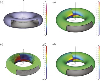
Colour representation of the resulting ${\it\phi}^{S}$ and S/S-currents $-\bar{{\it\sigma}}\boldsymbol{{\rm\nabla}}{\it\phi}^{S}$ . (a) The zoomed view on the wetting zone which contains the major part of the S/S-current. (b) The zoomed view on the sink zone with S/S currents converging to its centre. (c) The zoomed view on the source zone with S/S currents diverging from its centre. (d) Bottom view, showing the lack of the S/S-currents at the bottom part of the wall.

With these assumptions, the S/S-current is calculated by the SSC code. In turn, the SHL code calculates the eddy currents in the wall generated by the plasma kink deformation and by S/S-current. Together they represent the total surface current in the wall. What is missed at this stage of code development is the backward effect of these currents on the plasma shape and its surface currents. This important and complicated step is left for future development.

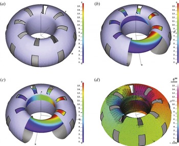
Figures 5 and 6 shows the calculations which mimic the wetting zone and Hiro currents due to WTKM during an AVDE. Figure 5(b) shows a toroidal plasma, shifted upward and perturbed by a $m/n=1/1$ kink perturbation. As a result, a wetting zone is created and displayed as a piece of plasma surface in front of the inner wall. The blue colour on the plasma surface indicates the direction of the surface current, opposite to the plasma current, while the red colour corresponds to the plasma surface currents in the same direction as the plasma current.

It is a fundamental result of the theory of the wall touching modes (Zakharov Reference Zakharov2008; Zakharov et al. Reference Zakharov, Galkin and Gerasimov2012) that the Hiro currents are negative (relative to the total plasma current). They determine the sign the source $j_{\bot }$ for S/S-currents as is reflected in figure 5(c) by colour of the wetting zone (red for positive and blue for the negative $j_{\bot }$ ). 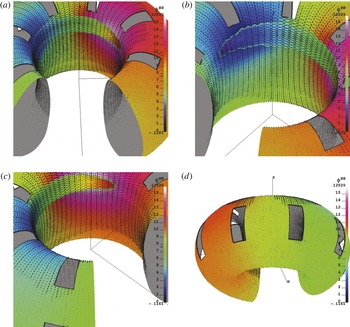As the simplest choice, $j_{\bot }$ is prescribed as uniform in the vertical direction, with the amplitude corresponding to the Hiro current entering the wetting zone at a particular azimuth, as shown in figure 5(c) by colours in the wetting zone. Figure 5(d) presents the solution to (2.2). Four frames in figure 6 show different views of the solution ${\it\phi}^{S}$ and the pattern of the S/S current density represented by the short straight lines. All calculations (35 840 triangles in this case) are made on a single processor mode on M3800 Dell laptop and it takes several seconds to calculate ${\it\phi}^{S}$ if the Cholesky decomposed matrix is given. The significant potential for code acceleration by using the cyclic matrix Fourier decomposition of Graphic Processor Units has not yet been used.

Figure 7.

Eddy and S/S-currents in the wall from a WTKM. (a) Wetting zone created by a shifted vertically toroidal plasma with a $m/n=1/1$ surface perturbation. The colour of the wall surface reflects the distribution of $A_{{\it\varphi}}$ component of the perturbed vector potential. (b) Eddy currents excited by the plasma perturbation. The colour corresponds to their stream function. (c) Eddy currents excited by both plasma perturbation and S/S current. The colour reflects the distribution of ${\it\phi}^{S}$ at the wall surface; (d) the total surface current with the S/S current as the dominant component.

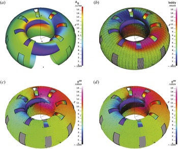
Four frames of figure 7 show the results of combined calculations by the SSC and SHL of the S/S and eddy currents in the wall. The colour of the wall surface in figure 7(a) displays the amplitude of the toroidal component of the vector potential $A_{{\it\varphi}}^{pl}$ of the plasma magnetic perturbation. The eddy current $i^{pl}$ due to the ‘ideal’ response of the wall to the plasma perturbed magnetic field is shown in figure 7(b). The colour of the wall surface reflects the value of the stream function $I$ of the eddy currents. Figure 7(c) displays the eddy current $i^{S}$ excited by the S/S-current, while the surface colour represents ${\it\phi}^{S}$ , as in figure 5(d).

The final figure 7(d) shows the total surface current, which includes both of the above mentioned eddy currents and the S/S-current. The colour of the surface is the same as in figure 7(c). This appears to be an important result of the present calculations in that the total surface current is dominated by the S/S-current due to the sharing of Hiro currents with the plasma. Thus, the relative average amplitudes of eddy currents relative to the S/S current are given by

(8.1a,b ) $$\begin{eqnarray}\displaystyle \frac{\sqrt{\displaystyle \int |\boldsymbol{{\rm\nabla}}{\it\phi}^{S}|^{2}\,\text{d}S}}{\sqrt{\displaystyle \int i^{2pl}\,\text{d}S}}=44.5,\quad \frac{\sqrt{\displaystyle \int |\boldsymbol{{\rm\nabla}}{\it\phi}^{S}|^{2}\,\text{d}S}}{\sqrt{\displaystyle \int i^{2S}\,\text{d}S}}=2.41, & & \displaystyle\end{eqnarray}$$

where the integration is over the wall surface.

These numbers reflect the fundamental physics of the WTKM (Zakharov et al. Reference Zakharov, Galkin and Gerasimov2012). The Hiro currents for the $m/n=1/1$ kink mode are not sensitive to the edge value of the safety factor $q_{a}$ and for a circular plasma with major and minor radii $R,a$ , are given simply by

(8.2) $$\begin{eqnarray}\displaystyle {\it\mu}_{0}\boldsymbol{i}^{Hiro}=-2\frac{B_{{\it\varphi}}}{R}{\it\xi}\left(1-\frac{1-q_{a}}{q_{a}}{\it\lambda}\right)\left(\boldsymbol{e}_{{\it\varphi}}+\frac{a}{R}\boldsymbol{e}_{{\it\omega}}\right)\cos ({\it\omega}-{\it\varphi}), & & \displaystyle\end{eqnarray}$$

where $\boldsymbol{e}_{{\it\omega}}$ is the poloidal unit vector on the plasma surface. The factor ${\it\lambda}<1$ in the second term, which contains the small factor $(1-q_{a})$ , takes into account the effect of the wall. In the present simulations $q_{a}=0.9$ , as could be realistically expected for the experimental situation in AVDEs. For any $q_{a}$ near the resonant level, $\boldsymbol{i}^{Hiro}$ are essentially determined by the first term of the equation.

At the same time, the magnetic field perturbation outside the plasma is proportional to the resonant factor $(1-q_{a})$

(8.3) $$\begin{eqnarray}\displaystyle rA_{{\it\varphi}}=\frac{a^{2}}{R{\it\rho}}{\it\xi}B_{{\it\varphi}}\frac{1-q_{a}}{q_{a}}\cos ({\it\theta}-{\it\varphi}), & & \displaystyle\end{eqnarray}$$

where ${\it\rho}$ is the polar radius counted from the plasma axis at ${\it\varphi}=\text{const}$ .

This difference in amplitude explains the dominant role of S/S-currents excited by Hiro currents in the wetting zone of the wall. The opposite direction with respect to the plasma current direction can explain the negative loop voltage spike appearing when the plasma touches the wall at the beginning of the disruptions.

9. Optimization of the solutions to the source/sink equation

As in the previous examples, given the source term $j_{\bot }$ , the (2.2) for the source/sink current can be solved in the entire domain separately from (2.4). At the same time, the representation of the source/sink current in terms of a source potential $-\bar{{\it\sigma}}\boldsymbol{{\rm\nabla}}{\it\phi}^{S}$ is essential only in the domain containing $j_{\bot }$ . Outside of this domain, the surface current is divergence free and both representations are valid. In particular, the uniform current density in a single triangle can be represented by

(9.1) $$\begin{eqnarray}\displaystyle \boldsymbol{i}=\frac{I_{a}\boldsymbol{r}_{cb}+I_{b}\boldsymbol{r}_{ac}+I_{c}\boldsymbol{r}_{ba}}{2S}=\langle \bar{{\it\sigma}}\rangle \left(\frac{{\it\phi}_{a}^{S}\boldsymbol{r}_{cb}+{\it\phi}_{b}^{S}\boldsymbol{r}_{ac}+{\it\phi}_{c}^{S}\boldsymbol{r}_{ba}}{2S}\times \boldsymbol{n}\right). & & \displaystyle\end{eqnarray}$$

The relations between the stream function $I$ and gradient ${\it\phi}^{S}$ representations are given by

(9.2) $$\begin{eqnarray}\displaystyle & \displaystyle I_{b}-I_{a}=({\it\phi}_{b}^{S}-{\it\phi}_{a}^{S})\frac{(\boldsymbol{r}_{ba}\boldsymbol{\cdot }\boldsymbol{r}_{ac})}{4S^{2}}+({\it\phi}_{c}^{S}-{\it\phi}_{a}^{S})\frac{(\boldsymbol{r}_{ba}\boldsymbol{\cdot }\boldsymbol{r}_{ba})}{4S^{2}}, & \displaystyle\end{eqnarray}$$

(9.3) $$\begin{eqnarray}\displaystyle & \displaystyle I_{c}-I_{a}=-({\it\phi}_{b}^{S}-{\it\phi}_{a}^{S})\frac{(\boldsymbol{r}_{ac}\boldsymbol{\cdot }\boldsymbol{r}_{ac})}{4S^{2}}-({\it\phi}_{c}^{S}-{\it\phi}_{a}^{S})\frac{(\boldsymbol{r}_{ba}\boldsymbol{\cdot }\boldsymbol{r}_{ac})}{4S^{2}}. & \displaystyle\end{eqnarray}$$

$I$

${\it\phi}^{S}$

$I_{a}=0$

${\it\phi}_{a}^{S}=0$

This dual representation opens an opportunity to solve the problem with the maximum use of the divergence-free representation of the surface current.

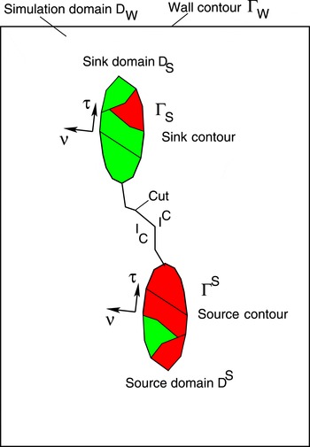
In this section we consider two cases: a single domain, containing both source and sink area; and two separated domains with a source and a sink area. The calculations in the previous sections give examples of both cases.

Figure 8.

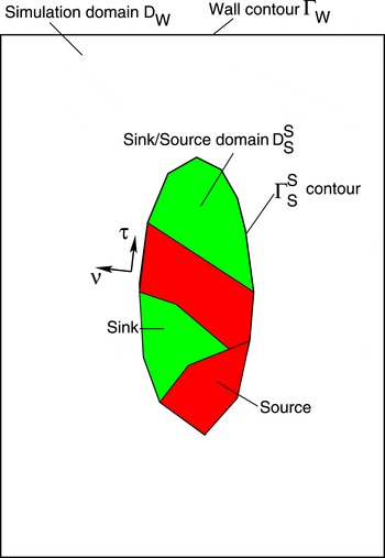
A single connected domain $D_{S}^{S}$ , limited by a contour ${\it\Gamma}_{S}^{S}$ with the source/sink current $j_{\bot }$ inside.

9.1. Single domain with source and sink inside

The simplified sketch of the domain topology is given in figure 8

(9.4) $$\begin{eqnarray}\displaystyle \int _{D_{S}^{S}}j_{\bot }\,\text{d}S=0. & & \displaystyle\end{eqnarray}$$

Vectors ${\bf\tau},{\bf\nu}$ are the unit vectors tangential and normal to ${\it\Gamma}_{S}^{S}$ , respectively

(9.5) $$\begin{eqnarray}\displaystyle ({\bf\nu}\times {\bf\tau})=\boldsymbol{n}. & & \displaystyle\end{eqnarray}$$

Inside ${\it\Gamma}_{S}^{S}$ the surface current density is represented by

(9.6) $$\begin{eqnarray}\displaystyle h\boldsymbol{j}_{S}^{S}=-\bar{{\it\sigma}}\boldsymbol{{\rm\nabla}}{\it\phi}^{S} & & \displaystyle\end{eqnarray}$$

and outside it

(9.7) $$\begin{eqnarray}\displaystyle h\boldsymbol{j}_{S}^{S}=(\boldsymbol{{\rm\nabla}}I_{S}^{S}\times \boldsymbol{n}). & & \displaystyle\end{eqnarray}$$

In this case, equation (2.2) for the source potential ${\it\phi}^{S}$ should be solved inside the $D_{S}^{S}$ domain

(9.8) $$\begin{eqnarray}\displaystyle (\boldsymbol{{\rm\nabla}}\boldsymbol{\cdot }(\bar{{\it\sigma}}\boldsymbol{{\rm\nabla}}{\it\phi}^{S}))|_{D_{S}^{S}}=-j_{\bot }. & & \displaystyle\end{eqnarray}$$

Outside $D_{S}^{S}$ (between ${\it\Gamma}_{S}^{S}$ and the wall contour ${\it\Gamma}_{W}$ ), a stream-function representation of the source/sink current is valid also

(9.9a,b ) $$\begin{eqnarray}\displaystyle -\!\bar{{\it\sigma}}\boldsymbol{{\rm\nabla}}{\it\phi}^{S}\equiv (\boldsymbol{{\rm\nabla}}I_{S}^{S}\times \boldsymbol{n}),\quad (\boldsymbol{{\rm\nabla}}\boldsymbol{\cdot }(\bar{{\it\eta}}\boldsymbol{{\rm\nabla}}I_{S}^{S}))=0 & & \displaystyle\end{eqnarray}$$

with the mixed Dirichlet–Neumann boundary conditions at ${\it\Gamma}_{S}^{S}$ , expressing the continuity of the current $h\boldsymbol{j}$ density at ${\it\Gamma}_{S}^{S}$ , and the Dirichlet condition at ${\it\Gamma}_{W}$

(9.10) $$\begin{eqnarray}\displaystyle & \displaystyle \bar{{\it\sigma}}({\bf\nu}\boldsymbol{\cdot }\boldsymbol{{\rm\nabla}}{\it\phi}^{S})|_{{\it\Gamma}_{S}^{S}}=-({\bf\tau}\boldsymbol{\cdot }\boldsymbol{{\rm\nabla}}I_{S}^{S})|_{{\it\Gamma}_{S}^{S}}, & \displaystyle\end{eqnarray}$$

(9.11) $$\begin{eqnarray}\displaystyle & \displaystyle \bar{{\it\sigma}}({\bf\tau}\boldsymbol{\cdot }\boldsymbol{{\rm\nabla}}{\it\phi}^{S})|_{{\it\Gamma}_{S}^{S}}=({\bf\nu}\boldsymbol{\cdot }\boldsymbol{{\rm\nabla}}I_{S}^{S})|_{{\it\Gamma}_{S}^{S}}, & \displaystyle\end{eqnarray}$$

(9.12) $$\begin{eqnarray}\displaystyle & \displaystyle I_{S}^{S}|_{{\it\Gamma}_{W}}=0. & \displaystyle\end{eqnarray}$$

This combined solution gives the solution for (2.2) in the entire domain.

Next, the contribution of the S/S-current $h\boldsymbol{j}_{S}^{S}$ to (2.4) (or to its variational form) can be calculated using Biot–Savart formulas, and then the (2.4) solved in the entire wall domain.

Figure 9.

Separate sink $D_{S}$ and source $D^{S}$ domains, limited by the contours ${\it\Gamma}_{S}$ and ${\it\Gamma}^{S}$ with $j_{\bot }$ inside.

As a result, the total surface current density will be given by

(9.13) $$\begin{eqnarray}\displaystyle h\boldsymbol{j}=\left\{\begin{array}{@{}ll@{}}(\boldsymbol{{\rm\nabla}}I\times \boldsymbol{n})-\bar{{\it\sigma}}\boldsymbol{{\rm\nabla}}{\it\phi}^{S} & \text{inside }D_{S}^{S},\\ (\boldsymbol{{\rm\nabla}}I\times \boldsymbol{n})+(\boldsymbol{{\rm\nabla}}I_{S}^{S}\times \boldsymbol{n}) & \text{between }{\it\Gamma}_{S}^{S}\text{ and }{\it\Gamma}_{W}.\end{array}\right. & & \displaystyle\end{eqnarray}$$

9.2. Two separated domains with sources/sinks

Figure 9 gives a simplified sketch of two domains. In the following notation, the superscript corresponds to the source and the subscript corresponds to the sink domain.

(9.14) $$\begin{eqnarray}\displaystyle & \displaystyle \int _{D^{S}}j_{\bot }\,\text{d}S=I^{S}\neq 0, & \displaystyle\end{eqnarray}$$

(9.15) $$\begin{eqnarray}\displaystyle & \displaystyle \int _{D_{S}}j_{\bot }\,\text{d}S=-I^{S}\neq 0, & \displaystyle\end{eqnarray}$$

(9.16) $$\begin{eqnarray}\displaystyle & \displaystyle \int _{D_{S}}j_{\bot }\,\text{d}S+\int _{D^{S}}j_{\bot }\,\text{d}S=0. & \displaystyle\end{eqnarray}$$

Vectors ${\bf\tau}_{S},{\bf\nu}_{S},{\bf\tau}^{S},{\bf\nu}^{S}$ are the unit vectors tangential and normal to ${\it\Gamma}_{S},{\it\Gamma}^{S}$ , respectively.

In this case, there is a non-zero current flow $I^{S}$ from $D^{S}$ to $D_{S}$ and a cut between the two domains is necessary to represent the divergence-free current $(\boldsymbol{{\rm\nabla}}I_{S}^{S}\times \boldsymbol{n})$ outside $D_{S},D^{S}$ . At the sides of the cut, its values $I_{C},I^{C}$ are different

(9.17) $$\begin{eqnarray}\displaystyle I_{C}=I^{C}+I^{S}. & & \displaystyle\end{eqnarray}$$

Otherwise, a similar problem with (2.2) inside the domains $D_{S},D^{S}$ for ${\it\phi}^{S}$ and (9.9) for $I_{S}^{S}$ outside of it and with mixed boundary conditions at ${\it\Gamma}^{S},{\it\Gamma}_{S}$ should be solved, as in the previous case.

9.3. A unified formulation for the surface currents

For practical implementation, $I_{S}^{S}$ can be consumed by the stream function $I$ , which is discontinuous (double valued at ${\it\Gamma}_{S}^{S}$ ) together with its normal derivative $({\bf\nu}\boldsymbol{\cdot }\boldsymbol{{\rm\nabla}}I)$ across ${\it\Gamma}_{S}^{S}$ . Using ‘ $e,i$ ’ superscripts in order to specify the external and internal values of discontinuous functions at the contour ${\it\Gamma}_{S}^{S}$ , we denote the two values of $I$ at ${\it\Gamma}_{S}^{S}$ by $I^{e},I^{i}$ .

The system of equations for the surface current can be written as a system of (2.2), (2.4)

(9.18) $$\begin{eqnarray}\displaystyle & \displaystyle (\boldsymbol{{\rm\nabla}}\boldsymbol{\cdot }(h\boldsymbol{j}))=-(\boldsymbol{{\rm\nabla}}\boldsymbol{\cdot }(\bar{{\it\sigma}}\boldsymbol{{\rm\nabla}}{\it\phi}^{S}))=-j_{\bot }\quad \text{inside }D_{S}^{S}, & \displaystyle\end{eqnarray}$$

(9.19) $$\begin{eqnarray}\displaystyle & \displaystyle (\boldsymbol{{\rm\nabla}}\boldsymbol{\cdot }(\bar{{\it\eta}}\boldsymbol{{\rm\nabla}}I))=\frac{\partial (B_{\bot }^{I}+B_{\bot }^{S})}{\partial t}+\frac{\partial (B_{\bot }^{pl}+B_{\bot }^{coil})}{\partial t}\quad \text{inside }{\it\Gamma}_{W},\text{ excluding the contour }{\it\Gamma}_{S}^{S}, & \displaystyle \nonumber\\ \displaystyle & & \displaystyle\end{eqnarray}$$

with mixed Dirichlet–Neumann boundary conditions at the source/sink contour ${\it\Gamma}_{S}^{S}$ and a Dirichlet condition at the wall contour ${\it\Gamma}_{W}$

(9.20) $$\begin{eqnarray}\displaystyle & \quad \hspace{-3.0pt}\displaystyle \bar{{\it\sigma}}({\bf\nu}\boldsymbol{\cdot }\boldsymbol{{\rm\nabla}}{\it\phi}^{S})=-[{\bf\tau}\boldsymbol{\cdot }\boldsymbol{{\rm\nabla}}(I^{e}-I^{i})]\quad \hspace{6.0pt}\text{at }{\it\Gamma}_{S}^{S}, & \displaystyle\end{eqnarray}$$

(9.21) $$\begin{eqnarray}\displaystyle & \displaystyle \bar{{\it\sigma}}({\bf\tau}\boldsymbol{\cdot }\boldsymbol{{\rm\nabla}}{\it\phi}^{S})=({\bf\nu}\boldsymbol{\cdot }\boldsymbol{{\rm\nabla}}I)^{e}-({\bf\nu}\boldsymbol{\cdot }\boldsymbol{{\rm\nabla}}I)^{i}\quad \text{at }{\it\Gamma}_{S}^{S}, & \displaystyle\end{eqnarray}$$

(9.22) $$\begin{eqnarray}\displaystyle & \displaystyle I=0\quad \text{at }{\it\Gamma}_{W}. & \displaystyle\end{eqnarray}$$

The resulting total surface current density is given by

(9.23) $$\begin{eqnarray}\displaystyle h\boldsymbol{j}=(\boldsymbol{{\rm\nabla}}I\times \boldsymbol{n})+\left\{\begin{array}{@{}ll@{}}-\bar{{\it\sigma}}\boldsymbol{{\rm\nabla}}{\it\phi}^{S} & \text{inside }D_{S}^{S},\\ 0 & \text{between }{\it\Gamma}_{S}^{S}\text{ and }{\it\Gamma}_{W}.\end{array}\right. & & \displaystyle\end{eqnarray}$$

The same problem can be formulated in terms of the following variational principle

(9.24a,b ) $$\begin{eqnarray}\displaystyle \frac{\partial W_{S}^{S}}{\partial {\it\phi}^{S}}=0,\quad \frac{\partial W^{I}}{\partial I}=0, & & \displaystyle\end{eqnarray}$$

where

(9.25) $$\begin{eqnarray}\displaystyle W^{I} & \equiv & \displaystyle \int _{D_{W}}\left\{\frac{\partial (\boldsymbol{{\rm\nabla}}I\times \boldsymbol{n})\boldsymbol{\cdot }(\boldsymbol{A}^{I+S})}{2\partial t}+\bar{{\it\eta}}\frac{|(\boldsymbol{{\rm\nabla}}I\times \boldsymbol{n})|^{2}}{2}+\left((\boldsymbol{{\rm\nabla}}I\times \boldsymbol{n})\boldsymbol{\cdot }\frac{\partial \boldsymbol{A}^{pl+coil}}{\partial t}\right)\right\}\text{d}S\nonumber\\ \displaystyle & & \displaystyle \quad +\,\oint _{{\it\Gamma}_{S}^{S}}(I^{e}-I^{i})({\bf\tau}\boldsymbol{\cdot }\boldsymbol{{\rm\nabla}}{\it\phi}^{S})\,\text{d}l,\end{eqnarray}$$

(9.26) $$\begin{eqnarray}\displaystyle & \displaystyle W_{S}^{S}\equiv \int _{D_{S}^{S}}\left\{\frac{\bar{{\it\sigma}}(\boldsymbol{{\rm\nabla}}{\it\phi}^{S})^{2}}{2}-j_{\bot }{\it\phi}^{S}\right\}\text{d}S+\oint _{{\it\Gamma}_{S}^{S}}{\it\phi}^{S}({\bf\tau}\boldsymbol{\cdot }\boldsymbol{{\rm\nabla}}I)\,\text{d}l, & \displaystyle\end{eqnarray}$$

(9.27) $$\begin{eqnarray}\displaystyle & \displaystyle \boldsymbol{A}^{I+S}(\boldsymbol{r})\equiv \int _{D_{W}}\frac{(\boldsymbol{{\rm\nabla}}I\times \boldsymbol{n})-\bar{{\it\sigma}}\boldsymbol{{\rm\nabla}}{\it\phi}^{S}}{|\boldsymbol{r}-\boldsymbol{r}^{\prime }|}\,\text{d}S^{\prime }. & \displaystyle\end{eqnarray}$$

10. Summary

A rigorous mathematical formulation of the surface current circuit equations in the thin wall limit is given. In the triangular representation of the wall surface, both divergence-free eddy and source/sink currents are represented by the same model of a uniform current density inside each triangle. This model is implemented in the SSC and the shell simulation code SHL.

The coupling of finite element matrix equations for both types of currents contains the same matrix elements of mutual capacitance $C_{ij}$ of two triangles ‘ $i,j$ ’

(10.1) $$\begin{eqnarray}\displaystyle C_{ij}\equiv \int _{{\it\Delta}_{i}}\int _{{\it\Delta}_{j}}\frac{\text{d}S_{i}\,\text{d}S_{j}}{|\boldsymbol{r}-\boldsymbol{r}^{\prime }|}, & & \displaystyle\end{eqnarray}$$

(10.2a−c ) $$\begin{eqnarray}\displaystyle M_{ij}^{II}=(\boldsymbol{i}_{i}\boldsymbol{\cdot }\boldsymbol{i}_{j})C_{ij},\quad M_{ij}^{IS}=\bar{{\it\sigma}}_{j}(\boldsymbol{i}_{i}\boldsymbol{\cdot }\boldsymbol{{\rm\nabla}}{\it\phi}_{j}^{S})C_{ij},\quad M_{ij}^{SS}=\bar{{\it\sigma}}_{i}\bar{{\it\sigma}}_{j}(\boldsymbol{{\rm\nabla}}{\it\phi}_{i}^{S}\boldsymbol{\cdot }\boldsymbol{{\rm\nabla}}{\it\phi}_{j}^{S})C_{ij}\quad & & \displaystyle\end{eqnarray}$$

(integration is performed over surfaces of two triangles) used for calculation of mutual inductance $M_{ij}^{II}$ between the divergence-free currents (as in SHL and STARWALL). The additional mutual inductances $M_{ij}^{IS}$ between eddy currents and source/sink currents, and $M_{ij}^{SS}$ between source/sink currents, use the same $C_{ij}$ . This common feature provides the basis for interfacing upon necessity of the SSC and SHL codes with other similar codes, such as STARWALL, or source/sink codes which are under development with an alternative approach.

The optimized formulation of the S/S-current problem for the typical tokamak situation of a localized wetting zone is presented. It is shown that the gradient representation can be used only in the wetting zone while the divergence-free stream-function representation of the surface current can used over the entire wall surface.

The numerical examples presented in the paper correspond to typical geometries of the wall and the wetting zone. In particular, the S/S and eddy currents generated by the Hiro current from the WTKM are modelled by both SSC and SHL codes.

Although the primary topic of the paper is the demonstration of the capabilities of two numerical codes in modelling the currents in 3-D walls, the simulations of the WTKM give strong support to the idea of explaining the negative voltage spike in tokamak disruptions by Hiro current excitation. This provides the additional motivation for further development of the presented model and the codes. In particular, a plasma physics model of HSoL should be developed for a realistic representation of the wetting zone and the path of the Hiro currents. Another step consists in interfacing the wall current codes SSC and SHL with plasma core codes, such as JOREK (Huysmans & Czarny Reference Huysmans and Czarny2007; Hoelzl et al. Reference Hoelzl, Merkel, Huysmans, Nardon, McAdams and Chapman2012, Reference Hoelzl, Huysmans, Merkel, Atanasiu, Lackner, Nardon, Aleuynikova, Liu, Strumberger and McAdams2014), NIMROD (Sovinec et al. Reference Sovinec, Glasser, Gianakon, Barnes, Nebel, Kruger, Schnack, Plimpton and Tarditi2004) or TMHD-based DSC and VDE codes (Zakharov et al. Reference Zakharov, Galkin and Gerasimov2012; Xiong et al. Reference Xiong, Xu, Wang, Zakharov and Li2015). This would allow for self-consistent simulations of plasma dynamics and plasma-wall interactions in tokamak disruptions.