Introduction
Over the last few decades, Wireless Communication (WC) has experienced a rapid boom in the deployment of electronic appliances, and further more development is expected [Reference Sharma and Bhatia1]. Effective WC techniques are considered as the driving force for global revolution. This mode of communication has fully transformed the way of living and created a fully connected society [Reference Wang, You, Yang, Zhou and Wang2]. WC domain encompasses a huge variety of WC devices and technologies, engages in digital connectivity, and hence it offers global coverage. The primary goal of this technology is to allow easy transfer of useful information between the endpoints that are not physically connected [Reference Sran and Sivia3]. Convenient accessibility, mobility, and constant and high-speed connectivity are the desirable characteristics of a modern WC system [Reference Prasad, Pardhasaradhi, Madhav, Isalm, Das and Ghzaoui4]. In the present times, modern electronic gadgets like mobile phones, laptops, tablets, mixer players, and other electronic products are the expected items that employ this technology [Reference Ahmad, Kabir and Bukhari5]. In addition, the rapid expansion of modern wireless technologies and rising demand for fast data communication have prompted the emergence of novel and innovative antenna designs [Reference Islam, Ali, Awan, Alzaidi, Alghamdi and Alathbah6]. In this digital age, designing of an antenna with salient features such as compactness, high data rate, and high fidelity for an efficient WC system is a challenging task. Huge progress in modern WC technologies has triggered a new domain of antenna designing, named as Fractal Antennas (FAs) [Reference Kaur and Sivia7]. The ever-growing advancements in antenna electromagnetics have pushed the fractal design approach to an extraordinary level. Implementation of FAs is an onerous task that requires numerous iterations, starting from a general conceptual strategy to the design implementation [Reference Das, Mitra and Chaudhuri8]. B. B. Mandelbrot is a famous French mathematician who firstly framed the word “fractal” [Reference Mark, Mishra, Mandal, Sarkar and Das9]. He had conducted huge research, analyzed numerous fragmented and cracked designs/shapes that exhibit self-similarity and scaling features. Fractal geometries are inspired by natural fractal patterns such as snowflakes, ice crystals, pineapples, broccoli, seashells, peacock fins, spiral galaxies, and so on [Reference Kaur and Malik10, Reference Mezaal, Eyyuboglu and Ali11]. Fractal design configurations offer electrical length enhancement associated with the patch without increasing the patch area [Reference Jindal, Sivia and Bindra12]. Hence, instead of employing numerous radiating elements for specific operational bands, a single component radiator can manage multiresonant bands and satisfy the requirements of WC [Reference Jain and Singh13]. As a consequence, FAs are considered as the key choice in modern communication systems as they help in achieving better performance characteristics.
Fractal based geometrical designs have been becoming more popular over the past few years. Different fractal configurations exhibiting significant size reduction and multiband behavior are described in [Reference Akkole and Vasudevan14–Reference Sharma, Sharma and Bhatia16]. A novel pentagonal FA implemented with modified coplanar ground was projected for Ultra WideBand (UWB) applications [Reference Singh, Kumar, Singh and Singh17]. The possessed peak gain was 2.2 dB and the claimed results were highly promising. S. Shandal et al. [Reference Shandal, Mezaal, Mosleh and Kadim18] described the theoretical analysis of a sophisticated circular patch resonator designed with fractalization method. The mentioned design gave two operational points (5.7 and 7.9 GHz) and the associated impedance bandwidth was 4.8 GHz. M. G. Siddiqui et al. [Reference Siddiqui, Devesh and Ansari19] suggested a modified A-shaped fractaled triangular geometry that shows its functionality for X, Ku, and K band applications. Moreover, the two-iterated configured geometry was scrutinized using cavity model method. The step-by-step evolution procedure of a modified inverted triangular structure was effectively characterized and reported in [Reference Kumari, Awasthi and Bansal20]. Two alphabetic cuts (H-cut and I-cut) embodied FA of volume = 50 × 60 × 1.6 mm3 was successfully realized for UWB applications [Reference Karanam and Kakkar21]. M. Marzouk et al. [Reference Marzouk, Nejdi, Youssef, Barua, Mohamed, Ahmad and Husseina22] discussed a new design of area 1020 mm2. The investigated frequency range was 3.2–7.5 GHz and the peak gain was 6.8 dB. In recent literature, numerous soft computing methodologies have been employed by distinct researchers and antenna designers to find the best analytical solutions for the complex antenna topologies [Reference Sran and Sivia23]. Depending on the interest, the authors utilized specific optimization techniques in their work. B. S. Dhaliwal et al. [Reference Dhaliwal, Kaur, Kaur and Pattnaik24] constructed a 1.47 mm thick fractal MIMO antenna with an Artificial Neural Network (ANN) approach. Good consistency among software produced and experimentally computed outcomes authenticated the recommended ANN approach. An ANN based small-scaled hybridized fractal design was created and verified experimentally for biomedical applications in [Reference Kaur and Sivia25]. S. Rajapriya et al. [Reference Rajapriya and Daniel26] illustrated a small-sized Hilbert curve fractal antenna embedded with a rectangular split ring resonator. The important geometric parameters were optimized with the demonstrated ANN approach. In [Reference Kaur, Krishan, Kaur and Sivia27], Invasive Weed Optimization based conglomerated fractal antenna was realized and its functional behavior was compared with the same antenna implemented using Harmony Search Algorithm (HSA). Y.A. Mohammed and D.K. Naji [Reference Mohammed and Naji28] effectively applied the concept of HSA in antenna arrays for sidelobe suppression. The usefulness of HSA approach for the optimal pattern synthesis of antenna arrays was illustrated in [Reference Guney and Onay29].
This research work is primarily concerned with the implementation and analysis of a HSA-ANN Ensembled integrated approach based modified dual staircase-shaped multiband fractal antenna. Using the developed hybrid algorithm, this meticulously engineered antenna is designed with an aim to achieve desired resonances and bandwidths in a controlled manner. For easy understanding, this paper is categorized into six sections. Section 2 emphasizes on the working principle and the adopted design criteria for the creation of the produced design. Section 3 offers detailed insights into the employed ANN Ensembled approach and HSA operational procedure. A detailed discussion including optimized outcomes, software generated and experimentally produced outcomes associated with the Realized DSSFA is demonstrated in Section 4. To justify the novelty of the constructed design in Section 5, the performance of the Realized DSSFA is compared with some previously manufactured antennas. At the end, concluding remarks related to the presented research work are briefly revealed in Section 6.
Antenna design methodology
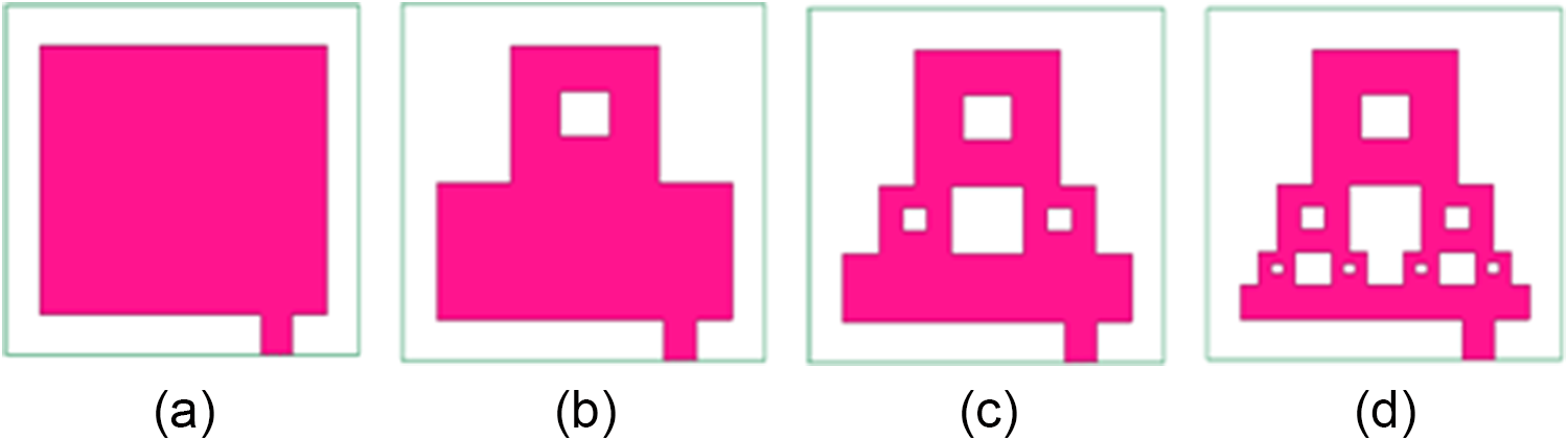
The improvised antenna is created iteratively by applying a staircase-shaped pattern on two opposite sides of the radiator along with a Sierpinski carpet (SC) fractal slot at the center of the upper-half portion. This meticulous design exhibits a symmetrical nature and multiband functionality. The detailed description of the step-by-step implementation of the Realized DSSFA is given in Fig. 1 (a–d). The key aspects associated with the design are particularly noteworthy.
Development stages of Realized DSSFA (a) Stage I, (b) Stage II, (c) Stage III, and (d) Stage IV.

The designed antenna is constructed physically on a Flame Retardant-4 (FR4) based dielectric slab of complete volume 26 × 32 × 1.6 mm3. The specifications of the chosen, handy and financially manageable substrate are dielectric constant, εr = 4.4, flexural strength = 60,000 psi, and Poisson’s ratio = 0.118 [Reference Sharma, Sharma and Bhatia16]. The geometrical construction begins with an initiator of size 20 × 26 mm2, as illustrated in Fig. 1(a) (indicated as Stage I). In the 1st iteration, two equal sized rectangular blocks of dimensions (length =  $\frac{1}{2}{\text{th}}$ of the patch length and width =
 $\frac{1}{4}{\text{th}}$ of the patch width) positioned at the top left and right corners, are etched from the parent geometry. Afterward, an SC fractal slot of dimensions “L S1” (
 $\frac{1}{6}{\text{th}}$ of the patch length) and “W S1” (
 $\frac{1}{6}{\text{th}}$ of the patch width) is embedded at the center of the upper-half portion of the geometry. The structure at this phase is named as Stage II (referred in Fig. 1b). The same design criterion is adopted for the development of Stage III (shown in Fig. 1c). Similarly, based on the above-said construction procedure, Stage IV (final shape, portrayed in Fig. 1d) is generated. The designed radiator is energized electromagnetically with a suitable 50 Ω microstrip feedline of dimensions “L F” and “W F”. Here, the feedline is placed at a point away from the center (towards the right side of the y-axis). The predicted value of feed position and ground length achieved using the respective heterogeneous ANN Ensembled Model (described in Section 4.1) is utilized in the design process. For improved impedance matching, a slot loaded ground plane of dimensions “L GD” and “W GD” mm2 is employed. Defected ground plane behaves as an impedance-matching element. It also offers modified current distribution and enhanced electromagnetic antenna characteristics. Further, it enables size reduction and multiband behavior. The resultant structure is named as modified Dual Staircase-Shaped Fractal Antenna (DSSFA). The complete structural arrangement of the Realized DSSFA (front and rear view) with labelled geometrical design parameters is illustrated in Fig. 2. The optimal design specifications of the Realized DSSFA are enlisted in Table 1.
Realized DSSFA (a) final geometry, and (b) defected ground plane.

Figure 2 Long description
The image A shows the final geometry of a Dual Staircase-Shaped Fractal Antenna (DSSFA) with various labeled dimensions. The structure includes multiple rectangular and square sections with dimensions labeled as L subscript 1, W subscript 1, L subscript 2, W subscript 2, L subscript 3, W subscript 3, LS subscript 1, WS subscript 1, LS subscript 2, WS subscript 2, LS subscript 3 and WS subscript 3. The overall width and height are labeled as W subscript SB and L subscript SB. The feedline dimensions are marked as L subscript F and W subscript F. The image B shows the defected ground plane with dimensions labeled as L subscript GD and W subscript GD. A slot is present in the ground plane, labeled with dimensions L subscript G1 and W subscript G1. The arrangement illustrates the structural design of the antenna and its ground plane, highlighting the specific geometric parameters involved in its construction.
Optimal design specifications of Realized DSSFA

Table 1 Long description
The table lists optimized geometric dimensions for a realized DSSFA design, giving named length and width parameters in millimeters. The largest values are WSB 32 mm and WGD 32 mm, followed by LSB 26 mm and LGD 19 mm. Mid sized dimensions include L1 10 mm, W1 13 mm, and LG1 10 mm, while L2 is 5 mm and W2 is 6.5 mm. Smaller features include LF 3.5 mm, WF 2.8 mm, W3 3.25 mm, and L3 2.5 mm. The smallest values are in the LS and WS series, ranging from LS3 0.833 mm and WS3 1.083 mm up to LS1 3.33 mm and WS1 4.33 mm. Overall, the design combines a few large baseline and guide dimensions with many much smaller segment dimensions, so small changes in the LS and WS values may represent fine features compared with the main body sizes.
All the parametric dimensions are in mm.
Formulation of HSA-ANN Ensembled based integrated strategy
This section describes the generation procedure of a HSA-ANN Ensembled hybrid technique utilized in the designing process of the Realized DSSFA. In the first phase, two distinct heterogeneous ANN Ensembled Models are developed for the prediction of two critical design parameters belonging to the projected design. In the second phase, HSA approach is applied for the optimization of operating points. The well-trained Ensembled Models are employed in this phase for the formulation of the fitness function.
Projected ANN Ensembled model
For the development and analysis of a projected antenna design, standard empirical formulas/numerical equations are not available because of the complex structural design process [Reference Dhaliwal and Pattnaik30]. Therefore, for such designs, soft computing approaches are very helpful as they offer acceptable answers within the specified range. One such approach is an ensembling of various ANNs bearing different structural characteristics. In some situations, a single ANN model is not able to produce good generalization for data sets that exhibit complexity and show random errors [Reference Dhaliwal and Pattnaik31]. Sometimes, a single ANN cannot handle large problems accurately. Therefore, there is a need to evaluate the outputs of different ANNs and then obtain the final output by averaging the previously computed outputs of each ANN model [Reference Haque, Rahman, Al-Bawri, Yusoff, Sharker, Abdulkawi, Saha, Paul and Zakariya32]. By doing so, the ensemble model shows good generalization performance in comparison to a single ANN.
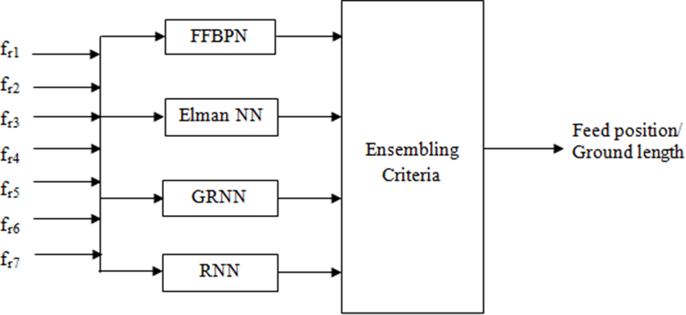
In this work, two different heterogeneous ANN Ensembled Models have been developed for two distinct cases. For the given resonant frequencies (“f r1,” “f r2,” “f r3,” “f r4,” “f r5,” “f r6,” and “f r7”), the first heterogeneous ANN Ensembled Model is developed to predict the feed position, whereas the second heterogeneous ANN Ensembled Model is implemented to predict the ground length [Reference Rajapriya and Daniel26]. In both cases, four different ANNs are chosen that include Feed Forward Back Propagation Network (FFBPN), Elman Neural Network (Elman NN), Generalized Regression Neural Network (GRNN), and Recurrent Neural Network (RNN). The outputs of these selected ANNs are aggregated and then the final ensembled output is taken by following the averaging method [Reference Dhaliwal and Pattnaik33]. A detailed description of the ANN ensembling process is given in Fig. 3. The specifications of the chosen ANN models utilized in the ensembled process are given in Table 2.
Heterogenous ANN Ensembled Model.

Specifications of the chosen ANN models employed in ensembled process

Table 2 Long description
The table lists four neural network models used in an ensemble and summarizes their hidden layer setup and key configuration details. FFBPN uses two hidden layers with 10 neurons and is configured with Trainlm training, random data distribution, Learngdm adaptive learning, and Tansig transfer. Elman NN uses two hidden layers with 12 neurons and uses Trainbfg training, with the same random distribution, Learngdm adaptive learning, and Tansig transfer. GRNN uses two hidden layers with 20 neurons and is characterized by a spread constant of 0.8. RNN uses two hidden layers with 23 neurons and a spread constant of 0.6. Across models, the number of neurons increases from 10 to 23, and only the first two models report training and transfer functions while the last two emphasize spread constants.
The first heterogeneous ANN Ensembled Model has seven inputs: “f r1” to “f r7” and one output: the corresponding feed position. Likewise, the second heterogeneous ANN Ensembled Model has seven inputs (“f r1” to “f r7”) and one output: the associated ground length. To generate the desired database, 90 DSSFAs are randomly created by choosing different feed positions. In the same manner, another set of 90 DSSFAs is generated randomly by taking different ground lengths. The above-said datasets are generated by varying feed positions between 18 and 26 mm (along y-axis) and ground lengths between 17 and 25 mm (along x-axis), respectively. In each case, 64 samples are defined for the training process and 26 samples are for the testing process. Here, for the proper selection of diverse training samples from the complete training database, the bootstrap aggregating method is employed. The function of this method is to create 4 different training subsets. The produced training subsets are utilized for the training of each ANN model. Thereafter, all the trained ANN models are tested using the provided test data and then ensembling is done.
Harmony search algorithm
Firstly introduced in the year 2001 by M. Kaur et al. [Reference Kaur, Krishan, Kaur and Sivia27], Harmony Search Algorithm (HSA) is a well-known and effective meta-heuristic search approach that utilizes the pivotal principles associated with musicians’ harmony improvisation. The instrument player repeatedly adjusts the pitch of the instrument by taking numerous combinations for the creation of the best possible outcome, termed as pleasing (best) harmony [Reference Mohammed and Naji28]. HSA employs a few adjustable parameters. HSA converges quickly to provide the best optimal solution corresponding to several difficult real-time optimization problems [Reference Guney and Onay29]. Harmony search illustrates solutions as harmonics by following the process of selection, pitch adjustment, and note creation (new) [Reference Yang and Kiang34]. These predetermined harmonics are stored in Harmony Memory (HM).
The optimization problem of interest is given below [Reference Kaur, Krishan, Kaur and Sivia27]:
 \begin{equation}Min.\left( {or\,Max} \right)\,\,\,\,\,\,\,\,\,\,\,\,f\left( {{x_1},\,{x_2}, \ldots \ldots \ldots \ldots {x_d}} \right)\end{equation}
where f corresponds to the specified fitness function and xi (i = 1, 2, …, d) corresponds to the decision variable i.
The step-wise description of the employed HSA is given as:
Step 1 Initialization of control parameters. The related control parameters such as Harmony Memory Size (HMS), Harmony Memory Considering Rate (HMCR), Pitch Adjustment Rate (PAR), and the fret width (FW) are defined and assigned initially [Reference Mohammed and Naji28]. HMS specifies the maximum number of harmonics referred by the musician. HMCR refers to the probability at which the musician considers the randomly chosen harmony stored in HM [Reference Kaur, Krishan, Kaur and Sivia27]. PAR represents the probability of adjusting the chosen harmony. The value exhibited by the parameters (HMCR, PAR) lies between 0 to 1. FW depicts the pitch adjustment bandwidth. HMCR is used to adjust the exploration, whereas PAR and FW are employed to adjust the exploitation [Reference Guney and Onay29].
Step 2 Initialization of Harmony Memory. In the possible solution (search) space, N harmonics are stochastically created and placed suitably in HM [Reference Yang and Kiang34]. Harmony corresponds to the set of notes decided by the musician. In particular, Harmony i can be represented as  $\left[ {{x_{i,1}}{x_{i,2}} \ldots \ldots \ldots {x_{i,d}}} \right]$. For HM initialization, the employed empirical formula is given below [Reference Kaur, Krishan, Kaur and Sivia27]:
 \begin{align}{x_{i,j}} &= {l_j} + rand\left( {{u_i} - {l_j}} \right) i = 1,2, \ldots \ldots \ldots .N \nonumber\\
j &= 1,2, \ldots \ldots \ldots .d\end{align}
where  ${l_j}$ depicts the lower bound related to the decision variable j and
 ${u_j}$ reveals the upper bound related to the same decision variable [Reference Mohammed and Naji28]. rand represents the randomly produced value in the span interval [0,1]. Table 3 delineates the representation of HM in which the column at the last reveals the fitness function value corresponding to each harmony [Reference Kaur, Krishan, Kaur and Sivia27].
Format of HM

Table 3 Long description
The table lays out a template for recording a set of candidate solutions called harmonies. Each row represents one harmony, identified by its row label, and contains a sequence of decision-variable entries across multiple columns. The decision-variable columns begin with the first and second variables, continue through intermediate variables, and end with the last variable. The final column records a single fitness value for each harmony. Rows are shown for Harmony 1, Harmony 2, and Harmony N, with an ellipsis row indicating additional harmonies in between. The entries are placeholders rather than actual numbers, so the table communicates structure and required fields, not performance comparisons or trends.
Step 3 Improvisation. In this step, a new harmony is improvised by following the process of recombination and mutation [Reference Guney and Onay29]. The newly created harmony is expressed as $\,{x_{new}} = \,\left[ {{x_{new,1}}{x_{new,2}} \ldots \ldots \ldots {x_{new,d}}} \right].$ Using HMCR, each component associated with the new harmony is examined. With a probability PAR, pitch adjustment is applied if the examined component belongs to the set of existing harmonics [Reference Kaur, Krishan, Kaur and Sivia27]. FW depicts the step size of the associated movement. All such actions result in the creation of new harmony [Reference Yang and Kiang34].
Step 4 Updating the Harmony Memory. The fitness value belonging to the new harmony is evaluated. Afterward, the examined fitness value and the fitness value related to the worst harmony are compared [Reference Kaur, Krishan, Kaur and Sivia27]. If the evaluated fitness corresponding to the new harmony is better than the worst member’s fitness then the new harmony replaces the worst harmony [Reference Guney and Onay29]. Contrarily, there is no need for such a replacement.
Step 5 Termination Criterion. The above-described two steps (steps 2 and 3) are repeated until the pre-defined termination criterion is met [Reference Kaur, Krishan, Kaur and Sivia27]. When this condition is fulfilled, the algorithm stops and the final outcome is noted.
Step 6 Final result. This step gives the optimal solution to the concerned optimization problem. The provided optimal answer corresponds to the best harmony.
For the implementation of Realized DSSFA, an HSA-ANN Ensembled integrated approach is developed to achieve the desired frequency bands (2.43, 3.61, 4.20, 7.71, 8.69, 12.90, and 14.41 GHz). Based on the pre-defined goals, the formulated fitness function associated with the HSA is described in Eq. (3) [Reference Kaur, Krishan, Kaur and Sivia27]. In the derived equation, trained heterogeneous ANN Ensembled Models are employed to provide the values of feed position and ground length. During the optimization process, the fitness function converges to a minimum value so that the Realized DSSFA can resonate at the defined operating bands.
 \begin{equation}{\text{Fitness function }} = {{\alpha }}{\left( {{F_{Pi}} - {F_{PANN}}} \right)^{1/2}}\, + \,{{\beta }}{\left( {{L_{GDi}} - {L_{GDANN}}} \right)^{1/2}}\end{equation}
where α and β correspond to the control variables
Results and discussion
To demonstrate the reliability and supremacy of the Realized DSSFA, numerical simulations, computational analysis and experimental investigations are thoroughly exemplified in this section.
Computational analysis using developed ANN ensembled models
In this subsection, the performance of the developed ANN Ensembled Models has been analyzed and compared with the selected ANN models. The two distinct heterogeneous ANN Ensembled Models have been applied for exact prediction of two preliminary design parameters associated with the Realized DSSFA, i.e., feed position and ground length. After a deep parametric analysis, training and test datasets are generated. The quality of these models is recorded by evaluating the value of Mean Computed Error (MCE), Mean Absolute Error (MAE), Mean Square Error (MSE), Root Mean Square Error (RMSE), and R-squared [Reference Dhaliwal and Pattnaik30]. All the above-said performance metrics are numerically computed by Eqs. (4–8) [Reference Haque, Rahman, Al-Bawri, Yusoff, Sharker, Abdulkawi, Saha, Paul and Zakariya32, Reference Elmezughi, Salih, Afullo and Duffy35].
 \begin{equation}MCE=\left|\frac1n\sum_{k=1}^n\left(O_k-{\widehat O}_k\right)\right|\end{equation}
 \begin{equation}MAE=\frac1n\sum_{k=1}^n\left|O_k-{\widehat O}_k\right|\end{equation}
 \begin{equation}MSE=\frac1n\sum_{k=1}^n\left(O_k-{\widehat O}_k\right)^2\end{equation}
 \begin{equation}RMSE=\sqrt{\frac1n\sum_{k=1}^n\left(O_k-{\widehat O}_k\right)^2}\end{equation}
 \begin{equation}R^2=1-\frac{\sum_{k=1}^n\left(O_k-{\widehat O}_k\right)^2}{\sum_{k=1}^n\left(O_k-\overset\_O\right)^2}\end{equation}
where  ${{\text{O}}_k}$ specifies the actual output,
 ${\widehat O}_k$ reveals the predicted output,
 $\overset\_O$ represents the mean output value, and n indicates the number of samples.
All the obtained results regarding the estimation of feed position for test data using different ANN models/First heterogenous ANN Ensembled Model are summarized in Table 4. The estimated value of feed position computed using different ANN models (FFBPN, Elman NN, GRNN, RNN), and the developed heterogenous ANN Ensembled Model (first one) is compared with the desired value. From Table 4, it is found that the examined value of MCE is 0.0040. Similarly, Table 5 illustrates all the resultant outcomes regarding the estimation of ground length for test data using different ANN models/Second heterogenous ANN Ensembled Model. Here, the value of ground length estimated using FFBPN, Elman NN, GRNN, RNN, and the developed heterogenous ANN Ensembled Model (second one) is compared with the desired value. Thereafter, the value of MCE is calculated and found as 0.5856. Generally, small value of MCE delineates high predictive accuracy, whereas large value indicates low predictive accuracy. Desired performance measures evaluated from distinct ANN models/First heterogenous ANN Ensembled Model in regard to the feed position estimation are described in Table 6. On the other hand, Table 7 summarizes the values of desired performance indicators evaluated from distinct ANN models/Second heterogenous ANN Ensembled Model in regard to the ground length estimation. Among all these presented ANN models, it is demonstrated that the resultant First/Second heterogenous ANN Ensembled Models reveal high prediction accuracy in comparison to other selected ANNs.
Estimation of feed position for test data using different ANN models/First heterogenous ANN Ensembled Model

Table 4 Long description
The table lists 26 test cases where seven resonant frequencies in gigahertz are used as inputs to estimate antenna feed position in millimeters. For each case, five model outputs are reported (FFBPN, Elman neural network, GRNN, RNN, and an ANN ensemble) alongside the desired feed position and the ensemble’s signed error. Desired feed positions range from 21.0 mm to 24.3 mm, while ensemble estimates span about 20.62 mm to 24.67 mm. The ensemble is very close to the target in several rows, including test 23 where the error is near zero and test 16 where the error is only a few hundredths of a millimeter. The largest deviations occur in test 2 (ensemble about 0.68 mm below the desired 21.3 mm) and test 13 (ensemble about 0.52 mm above the desired 22.7 mm), with other notable differences in tests 17 and 25. Individual models sometimes diverge more strongly than the ensemble, such as Elman neural network around 25.77 mm in test 22 and RNN around 26.13 mm in test 25, while the ensemble remains closer to the desired values. Overall, the ensemble’s mean absolute error is reported as 0.0040, but this summary should be interpreted cautiously because it appears much smaller than many of the per-row errors shown.
Estimation of ground length for test data using different ANN models/Second heterogenous ANN Ensembled Model

Table 5 Long description
The table lists 26 test cases with seven resonant-frequency inputs (fr1 through fr7, in GHz) and compares predicted ground length (in mm) from five neural-network approaches: FFBPN, Elman NN, GRNN, RNN, and an ANN ensemble. For each case, the desired ground length is provided along with the ensemble’s computed error, allowing direct accuracy checking. Desired ground length increases from 17.0 mm in the first case to 23.15 mm in the last case, while the ensemble predictions generally track this rise. The ensemble error is negative in most rows, indicating the ensemble typically predicts a slightly larger ground length than desired. The largest magnitude error occurs in case 1 at about minus 1.41 mm; the closest matches are small positive errors around plus 0.03 mm in case 18 and plus 0.07 mm in case 26, and the largest positive error is about plus 0.25 mm in case 24. Across all rows, the mean absolute computed error reported for the ensemble is about 0.59 mm. Individual model outputs vary by row, sometimes differing by more than a millimeter from each other, so comparisons should focus on the desired value and the ensemble error column rather than any single model’s absolute scale.
Performance measures obtained from different ANN models/First heterogenous ANN Ensembled Model in regard to feed position estimation

Table 6 Long description
The table compares five neural network approaches for feed position estimation using MCE, MAE, MSE, RMSE, and R-squared percent. The ANN ensemble has the strongest overall performance, with the lowest MCE at 0.0040, MAE at 0.0002, MSE at 0.0897, RMSE at 0.2995, and the highest R-squared at 98 percent. FFBPN is the next best, with similarly low MAE at 0.0002 and high R-squared at 96 percent, but slightly higher MSE at 0.0962 and RMSE at 0.3101. Elman NN and GRNN show midrange accuracy, with R-squared values of 93 and 94 percent and RMSE values of 0.3180 and 0.3933, respectively. RNN performs worst overall, with the highest MCE at 0.1670, highest MAE at 0.0073, and the lowest R-squared at 92 percent. Overall, lower error metrics align with higher R-squared, suggesting the ensemble improves fit compared with individual models; results should be interpreted in the context of the same dataset and evaluation setup.
Performance measures obtained from different ANN models/Second heterogenous ANN Ensembled Model in regard to ground length estimation

Table 7 Long description
The table compares five neural network approaches for ground length estimation using MCE, MAE, MSE, RMSE, and R-squared percent. The ANN Ensemble has the strongest overall results, with the highest R-squared at 96 percent and the lowest MCE at 0.5856; it also has the lowest MSE at 0.5382 and RMSE at 0.7336. FFBPN is close in MCE at 0.5875 and has a very small MAE at 0.0315, but its MSE and RMSE are higher at 0.9740 and 0.9869, and its R-squared is 95 percent. RNN ranks next by fit, with R-squared at 94 percent and the lowest MSE and RMSE among the non-ensemble models at 0.7025 and 0.8381. Elman NN and GRNN show lower fit, with R-squared at 93 and 92 percent, and both have MAE just over 1.03; GRNN also has the highest MSE at 1.2416 and RMSE at 1.1143. Because the error metrics use different scales and definitions, comparisons should focus on relative ranking within each metric rather than treating all metrics as directly interchangeable.
The graphical representation of MCE obtained using the selected ANN models/First heterogenous ANN Ensembled Model against number of test samples in regard to feed position estimation is given in Fig. 4. The values of MCE obtained using selected ANN models/Second heterogenous ANN Ensembled Model against number of test samples in regard to ground length estimation are graphically delineated in Fig. 5. Performance assessment measures (MAE, MSE, RMSE, and R-squared(%)) obtained from all selected ANN models/First heterogenous ANN Ensembled Model in regard to feed position estimation are displayed in Fig. 6(a–d). Similarly, the critical performance assessment measures (MAE, MSE, RMSE, and R-squared [%]) obtained from the selected ANN models/Second heterogenous ANN Ensembled Model in regard to ground length estimation are displayed statistically in Fig. 7(a–d).
MCE against number of test samples in regard to feed position estimation.

Figure 4 Long description
The graph plots MCE in regard to feed position on the vertical axis, ranging from approximately negative 0.5 to positive 0.5, with no units stated. The horizontal axis represents the number of test samples, ranging from 0 to 25 in increments of 5. Five model series are plotted, each visually distinguished by line style as listed in the legend: FFBPN shown as a dashed line, Elman NN shown as a dotted line, GRNN shown as a dash-dotted line, RNN shown as a solid line and ANN Ensemble shown as a bold dashed line. All five lines fluctuate above and below zero across the full sample range, indicating both positive and negative error values throughout. Notable peaks reaching close to positive 0.5 and troughs reaching close to negative 0.5 are visible across multiple series, particularly in the range of samples 5 through 20. The ANN Ensemble line appears to remain closer to zero across more sample points compared to the individual model lines, while FFBPN and RNN show wider swings at several intervals. Around samples 10 and 15, multiple lines spike simultaneously, suggesting shared variability at those points. The lines do not show a clear convergence or divergence pattern as the number of test samples increases from 0 to 25. The overall spread of all five series remains within the negative 0.5 to positive 0.5 range throughout the entire horizontal axis.
MCE against number of test samples in regard to ground length estimation.

Performance assessment measures obtained from selected ANN models/First heterogenous ANN Ensembled Model in regard to feed position estimation (a) MAE, (b) MSE, (c) RMSE, and (d) R-squared (%).

Figure 6 Long description
The image A showing a bar graph. The horizontal axis label is Type of Neural Network. The categories are FFBPN, Elman NN, GRNN, RNN, ANN Ensemble. The vertical axis label is Mean Absolute Error. The vertical axis range is 0 to 10. The bar heights are: FFBPN about 0.2, Elman NN about 0.1, GRNN about 0.8, RNN about 9.0, ANN Ensemble about 0.1. The image B showing a bar graph. The horizontal axis label is Type of Neural Network. The categories are FFBPN, Elman NN, GRNN, RNN, ANN Ensemble. The vertical axis label is Mean Square Error. The vertical axis range is 0 to 0.2. The bar heights are: FFBPN about 0.10, Elman NN about 0.10, GRNN about 0.15, RNN about 0.13, ANN Ensemble about 0.09. The image C showing a bar graph. The horizontal axis label is Type of Neural Network. The categories are FFBPN, Elman NN, GRNN, RNN, ANN Ensemble. The vertical axis label is Root Mean Square Error. The vertical axis range is 0 to 0.4. The bar heights are: FFBPN about 0.30, Elman NN about 0.31, GRNN about 0.39, RNN about 0.36, ANN Ensemble about 0.29. The image D showing a bar graph. The horizontal axis label is Type of Neural Network. The categories are FFBPN, Elman NN, GRNN, RNN, ANN Ensemble. The vertical axis label is R squared. The vertical axis range is 0 to 100. The bar heights are: FFBPN about 98, Elman NN about 97, GRNN about 98, RNN about 97, ANN Ensemble about 99.
Performance assessment measures obtained from different ANN models/Second heterogenous ANN Ensembled Model ANN Ensemble in regard to ground length estimation (a) MAE, (b) MSE, (c) RMSE, and (d) R-squared(%).

Figure 7 Long description
The image A showing a bar graph. The horizontal axis label is Type of Neural Network. The vertical axis label is Mean Absolute Error in Feed Position Estimation. The horizontal axis categories, left to right, are FFBPN, Elman NN, GRNN, RNN, ANN Ensemble. The vertical axis range is 0 to 1.2. The bar heights are: FFBPN 1.0, Elman NN 1.0, GRNN 1.0, RNN 1.0, ANN Ensemble 1.0. The image B showing a bar graph. The horizontal axis label is Type of Neural Network. The vertical axis label is Mean Square Error in Feed Position Estimation. The horizontal axis categories, left to right, are FFBPN, Elman NN, GRNN, RNN, ANN Ensemble. The vertical axis range is 0 to 1.4. The bar heights are: FFBPN 1.0, Elman NN 0.8, GRNN 1.2, RNN 0.7, ANN Ensemble 0.6. The image C showing a bar graph. The horizontal axis label is Type of Neural Network. The vertical axis label is Root Mean Square Error in Feed Position Estimation. The horizontal axis categories, left to right, are FFBPN, Elman NN, GRNN, RNN, ANN Ensemble. The vertical axis range is 0 to 1.2. The bar heights are: FFBPN 1.0, Elman NN 0.9, GRNN 1.1, RNN 0.8, ANN Ensemble 0.7. The image D showing a bar graph. The horizontal axis label is Type of Neural Network. The vertical axis label is R squared in Feed Position Estimation. The horizontal axis categories, left to right, are FFBPN, Elman NN, GRNN, RNN, ANN Ensemble. The vertical axis range is 0 to 100. The bar heights are: FFBPN 95, Elman NN 94, GRNN 93, RNN 95, ANN Ensemble 96.
HSA-ANN Ensembled based integrated approach results
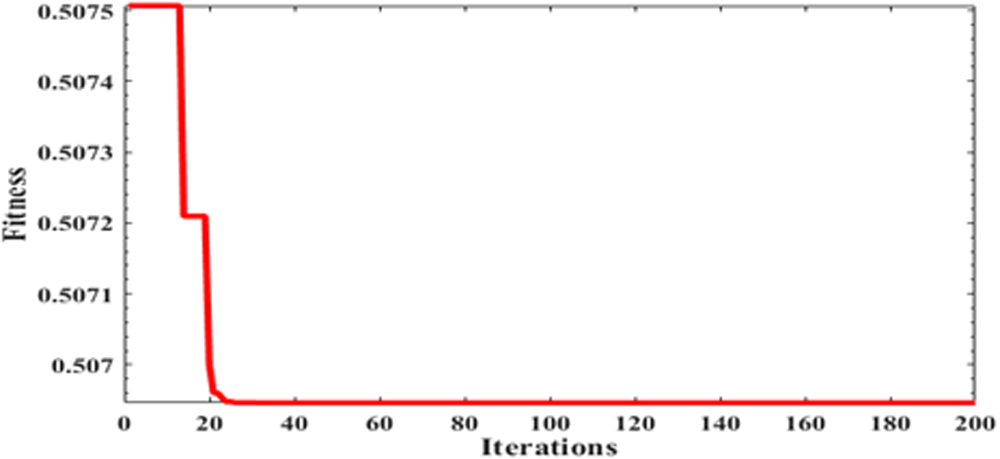
In HSA, number of harmonics “N” is assumed as 18 and the maximum number of iterations is taken as 200. The initially specified values of “HMS,” “HMCR,” “PAR,” and “FW” are 36, 0.95, 0.7, and 0.07, respectively. Effective hyperparameter tuning largely depends on the control on these parameters in order to balance global exploration and local exploitation. Hence, it helps in achieving improved convergence reliability. Optimization results characterize that the recommended hybrid algorithm converges to an value of 0.5069 after 24 iterations, as depicted in Fig. 8. The examined optimized values of “f r1,” “f r2,” “f r3,” “f r4,” “f r5,” “f r6,” and “f r7” are 2.4256, 3.6081, 4.2115, 7.7216, 8.6884, 12.8992, and 14.4009 GHz, respectively.
Fitness value associated with the HSA-ANN Ensembled based integrated approach.

Realized DSSFA results
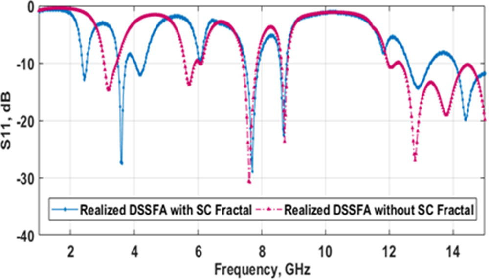
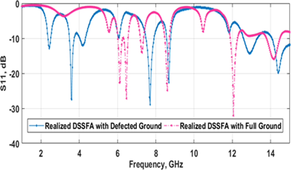
The design, characterization and implementation of the aforementioned antenna structure are carried out using an efficient simulation tool, v.15 Ansoft High-Frequency Structure Simulator (HFSS) [Reference Kaur and Sivia7]. The innovative and uncomplicated fractal geometry exhibits two salient features: concision and multiband operation [Reference Balanis36]. For analysis purposes, the spanning range chosen is 1 to 15 GHz. Figure 9 explicates the S11 characteristics of the Realized DSSFA at three different development stages. Results demonstrate that Stage II (1st iteration) produces two resonant bands, centered at 2.94 and 3.86 GHz with −10 dB impedance bandwidth (IBW) of 5.4% (2.86–3.02 GHz) and 5.7% (3.75-3.97 GHz), respectively. Subsequently, at Stage III (2nd iteration), six operational bands are examined. The recognized resonant points are 2.52, 3.55, 4.17, 7.87, 8.86, and 11.30 GHz. The noted Voltage Standing Wave Ratio (VSWR) values are ≤2, claiming good impedance matching. The final design (Stage IV/3rd iteration/Realized DSSFA) resonates at seven points within the above-specified frequency range. First band [Band-1] spans from 2.35 to 2.52 GHz, centered at 2.43 GHz and offers −10 dB IBW of 6.9%. Second band [Band-2] is centered at 3.61 GHz with a spanning range of 3.47–3.75 GHz (−10 dB IBW = 7.7%). Likewise, the Third band [Band-3] resonates at 4.20 GHz and the S11 is −12.05 dB. Fourth band [Band-4] lies in the range of 7.48-7.90 GHz. Here, the resonance is observed at 7.71 GHz. The linked S11 and VSWR are −28.84 dB and 1.07, respectively. Fifth band [Band-5] has a dominant frequency = 8.69 GHz and −10 dB IBW = 2.3%. The resonance and S11 associated with the sixth band [Band-6] is 12.90 GHz and −14.28 dB, respectively. The prominent resonance related to the seventh band [Band-7] is 14.41 GHz. The corresponding S11 is −19.82 dB and the −10 dB IBW is greater than 6.4%. Importantly, as a proof of concept, resonance lowering and enhancement in operational bands have been examined from Fig. 9. Additionally, the demonstrated fractal configuration offers a 33% size reduction. For a more reasonable explanation, performance comparison between three different development stages is illustrated in Table 8. Moreover, the S11 characteristics of the Realized DSSFA with/without incorporation of SC fractal are compared in Fig. 10. From this plot, it can be inferred that Realized DSSFA without incorporation of SC fractal offers six resonant bands, whereas the SC fractal incorporated projected design produces seven resonant bands. For more understanding, S11 characteristics of the Realized DSSFA with Defected Ground/Full Ground are compared in Fig. 11.
S11 characteristics of the Realized DSSFA at three different development stages.

Figure 9 Long description
S11 dB The x-axis is labeled Frequency GHz, with tick labels at 2, 4, 6, 8, 10, 12 and 14. The y-axis is labeled S subscript 11 dB, with tick labels at 0, minus 10, minus 20 and minus 30. A legend inside the plot lists three curves: Stage II, Stage III and Realized DSSFA (Stage IV). Stage II is drawn as a dashed curve. It shows two main dips: one near 3 gigahertz reaching close to minus 30 decibel and a second dip near 4 gigahertz reaching around minus 20 decibel. Outside these dips, the curve stays near 0 decibel. Stage III is drawn as a solid curve. It shows multiple dips: one near 2.5 gigahertz, additional dips between about 3 and 4.5 gigahertz and further dips between about 7.5 and 12 gigahertz. Several of these dips reach below minus 10 decibel, with the deepest dip near 6 gigahertz reaching close to minus 30 decibel. Realized DSSFA (Stage IV) is drawn as a solid curve. It shows several dips across the band: dips near about 2.4 gigahertz, around 3.6 gigahertz, around 4.2 gigahertz, around 7.7 gigahertz, around 8.7 gigahertz, around 12.9 gigahertz and around 14.4 gigahertz. The dip near about 7.7 gigahertz reaches close to minus 30 decibel, while other dips are mostly between minus 10 and minus 20 decibel.
S11 characteristics of the Realized DSSFA with/without incorporation of SC fractal.

Figure 10 Long description
The table lists multiple operating bands for three design stages, giving lower, resonant, and upper frequencies in gigahertz along with return loss S11 in decibels, bandwidth ratio, and VSWR. Stage II reports two bands: around 2.94 GHz with S11 about minus 11.69 dB and VSWR 1.74, and around 3.86 GHz with S11 about minus 15.95 dB and VSWR 1.38. Stage III expands to six bands from about 2.52 to 11.30 GHz, with its best match at about 11.30 GHz where S11 is about minus 29.60 dB and VSWR 1.06; another strong band is near 8.86 GHz with S11 about minus 22.50 dB and VSWR 1.17. Stage IV also covers seven bands from about 2.43 to 14.41 GHz, including very low S11 near 7.71 GHz at about minus 28.84 dB with VSWR 1.07 and near 3.61 GHz at about minus 27.43 dB with VSWR 1.08. Most bandwidth ratios cluster close to 1.02 to 1.09, with the final Stage IV row indicating an upper frequency above 15.00 GHz and a bandwidth ratio above 1.07. Overall, later stages generally show improved matching, reflected by more negative S11 values and VSWR values closer to 1, though performance varies by band.
S11 characteristics of the Realized DSSFA with Defected Ground/Full Ground.

Performance comparison between three different development stages

Table 8 Long description
The table lists multiple operating bands for three design stages, giving lower, resonant, and upper frequencies in gigahertz along with return loss S11 in decibels, bandwidth ratio, and VSWR. Stage II reports two bands: around 2.94 GHz with S11 about minus 11.69 dB and VSWR 1.74, and around 3.86 GHz with S11 about minus 15.95 dB and VSWR 1.38. Stage III expands to six bands from about 2.52 to 11.30 GHz, with its best match at about 11.30 GHz where S11 is about minus 29.60 dB and VSWR 1.06; another strong band is near 8.86 GHz with S11 about minus 22.50 dB and VSWR 1.17. Stage IV also covers seven bands from about 2.43 to 14.41 GHz, including very low S11 near 7.71 GHz at about minus 28.84 dB with VSWR 1.07 and near 3.61 GHz at about minus 27.43 dB with VSWR 1.08. Most bandwidth ratios cluster close to 1.02 to 1.09, with the final Stage IV row indicating an upper frequency above 15.00 GHz and a bandwidth ratio above 1.07. Overall, later stages generally show improved matching, reflected by more negative S11 values and VSWR values closer to 1, though performance varies by band.
Based on the dimensional geometry, as portrayed in Fig. 2, the antenna is fabricated. The hardware model of the Realized DSSFA joined with a suitable 50 Ω connector is portrayed in Fig. 12. The precisely constructed antenna structure is employed for experimentation. S11 characteristics are extracted using an Analyzer present in the microwave laboratory. For clear perception, the computed S11 values (software generated/experimentally extracted) are illustrated in Fig. 13. Practically computed measurements depict that the hardware model produces resonance at 2.48, 3.58, 4.25, 7.65, 8.74, 11.83, and 14.44 GHz with an associated Bandwidth Ratio (BWR) of 1.07, 1.07, 1.07, 1.04, 1.02, 1.02, and 1.06. After careful examination of the plot, a good resemblance between the software generated and experimentally extracted values is noted. Minor deviations are due to the measured apparatus errors, human errors, substrate inconsistency, disturbed environmental conditions, and insertion losses of connector and cable [Reference Regulagadda and Kumari37]. Hence, the experimental observations clearly reveal that the suggested design is an excellent competitor for Wireless Local Area Network (WLAN) (IEEE 802.11 b/g/n), Energy harvesting, Industrial, Scientific and Medical (ISM) band, Radio Frequency Identification (RFID), Amateur radio, Maritime mobile, Fixed mobile except aeronautical mobile, Direct broadcast satellite, Radio astronomy, Radio navigation, and Space research.
FR4 based developed DSSFA (a) Front side, and (b) Back side.

Simulated and experimentally extracted S11 behavior of the Realized DSSFA.

The working mechanism of the Realized DSSFA can be clearly examined by plotting the current distribution plots at six investigated resonances, namely, 2.43, 4.20, 7.71, 8.69, 12.90, and 14.41 GHz, as demonstrated in Fig. 14. In this investigation, it is possible to comprehend the regions that contribute to multiband frequencies [Reference Yang and Kiang34]. At 2.43 GHz, the current flow is prominent at the lower right portion of the designed patch. On the other side, the lower left and upper portions have weak currents. At 4.20 GHz, maximum circulation of current is around/near the center portion of the patch and the feed. Corresponding to 7.71/8.69 GHz, current is more concentrated at the lower, upper right portion of the radiator and the feed. At higher resonances (12.90/14.41 GHz), current is homogenously dispersed at the Realized DSSFA’s surface. From Fig. 14(a–f), it can be inferred that the etched fractal slots perturb the current path resulting in the appearance of additional resonances at higher values without increasing the antenna size. For the far-field analysis, reliable and consistent experimentation is done in an anechoic chamber. A standard pyramidal horn antenna bearing characteristics such as gain, “G T” = 8.5 dB and transmitting power, “P T” = 1 mW works as a reference antenna. The manufactured prototype is placed at the opposite end of the standard antenna device. The outcomes are recorded step-wise by varying the rotation angle from 0° to 360°. To eliminate the reflections, anechoic absorbing material has been utilized during the measurement process. Figure 15 reveals the comparison of experimentally extracted and software generated radiation patterns at six chosen resonant points. It is worth noting that at the claimed lower resonant points (2.43, 4.20, and 7.71 GHz), partially deformed omnidirectional patterns are examined, as depicted in Fig. 15(a–c). However, for higher resonant points (8.69, 12.90, and 14.41 GHz), generation of higher order modes causes the appearance of deformed butterfly (arbitrary bidirectional) patterns (portrayed in Fig. 15d–f). Gain computation at each resonance is done by applying the Friis transmission formula. Figure 16 portrays the simulated and practically revealed gain and efficiency values associated with the Realized DSSFA. The presented figure reports that the Realized DSSFA gives an experimental gain of 8.25, 5.16, 5.47, 4.08, 3.35, 5.56, and 8.49 dB at the targeted frequency points (2.48, 3.58, 4.25, 7.65, 8.74, 11.83, and 14.44 GHz), respectively. It can be conferred that the computed gain values are highly remarkable. Similarly, the described structure produces experimental efficiency of 86.26%, 90.47%, 83.75%, 69.19%, 69.37%, 93.18%, and 87.16% at the above-said frequency points. Here, it is recognized that the experimentally extracted gain and efficiency values are found close to the software computed outcomes. At last, all the examined performance metrics (simulated and measured) associated with the Realized DSSFA are compiled in Table 9. Based on all these outcomes, it can be undoubtedly stated that the manufactured model with notable features exhibits compactness, multifunctionality, bandwidth as well as high gain and efficiency.
Current distribution on Realized DSSFA’s surface at (a) 2.43, (b) 4.20, (c) 7.71, (d) 8.69, (e) 12.90, and (f) 14.41 GHz operational frequency points.

Figure 14 Long description
The image shows six 2D false-color spatial maps labeled a through f, each displaying the surface current distribution on the Realized DSSFA geometry at a specific operating frequency. The plotted quantity is surface current intensity in A per m superscript 2, shown using a colorbar scale on the left side of each map. The colorbar ranges from low values at the cool end to high values at the warm end. These are not X-Y axis charts; they are spatial maps of the antenna surface showing where current concentrates at each frequency. No excitation port conditions are labeled in the image. Image a corresponds to 2.43 GHz. The colorbar scale visible in this panel spans approximately 1.779 times 10 superscript plus 2 at the top to 1.779 times 10 superscript minus 4 at the bottom. Peak current intensity is concentrated near the feed point and the lower patch edge region. The outer perimeter and slot regions away from the feed show low intensity. Image b corresponds to 4.20 GHz. Peak current is concentrated near the feed line and the central patch region, with the slot edges showing moderate intensity. Regions along the outer perimeter of the patch show low intensity. Image c corresponds to 7.71 GHz. High current intensity appears near the feed point and along the upper patch edge and slot boundaries. Other surface regions show reduced intensity relative to these hotspots. Image d corresponds to 8.69 GHz. The distribution is similar to image c, with peak intensity near the feed point and the upper patch edge. Slot boundaries again show elevated intensity compared to the remaining surface area. Image e corresponds to 12.90 GHz. Current intensity is more widely distributed across the patch surface, with hotspots appearing near multiple slot edges and the feed region simultaneously. The contrast between peak and low regions is reduced compared to lower frequency panels. Image f corresponds to 14.41 GHz. Current intensity appears distributed across the full antenna surface including slot edges, patch corners and the feed region. The distribution is more uniform relative to earlier panels, with no single dominant hotspot region.
Simulated/software generated (solid line in blue and red color) and measured/experimentally extracted (dashed line in pink and green color) radiation patterns in regard to E and H planes of Realized DSSFA (a) 2.43, (b) 4.20, (c) 7.71, (d) 8.69, (e) 12.90, and (f) 14.41 GHz operational frequency points.

Figure 15 Long description
The image consists of six polar plots comparing simulated and measured radiation patterns for the Realized DSSFA at different frequencies. Each plot shows angles in degrees around the polar axis and gain in decibels on the radial rings. Simulated patterns are shown with solid lines, while measured patterns are shown with dashed lines. (a) At 2.43 GHz, the pattern shows a main lobe directed around 0 degrees with minor lobes. (b) At 4.20 GHz, the main lobe is more pronounced, with reduced sidelobes. (c) At 7.71 GHz, the pattern becomes more complex with multiple lobes. (d) At 8.69 GHz, the main lobe shifts slightly, showing increased complexity. (e) At 12.90 GHz, the pattern displays a broad main lobe with several smaller lobes. (f) At 14.41 GHz, the pattern is highly intricate with multiple lobes. The plots illustrate the agreement and discrepancies between simulated and measured data, highlighting changes in lobe shapes and directions across frequencies.
Simulated and practically revealed gain and efficiency values of the Realized DSSFA.

Figure 16 Long description
Simulated Gain → Measured Gain Simulated Efficiency → Measured Efficiency. A mixed line graph with four plotted lines and a legend at the top. The x-axis is labeled Frequency, GHz, with tick labels at 2, 4, 6, 8, 10, 12 and 14. The left y-axis is labeled Gain, dB, with tick labels at 2, 4, 6, 8, 10 and 12. The right y-axis is labeled Efficiency, %, with tick labels at 60, 70, 80, 90 and 100. Simulated Gain is shown with square markers at approximately: 2 GHz about 9.5 dB; 4 GHz about 7.0 dB; 8 GHz about 4.0 dB; 12 GHz about 6.5 dB; 14 GHz about 9.0 dB. Measured Gain is shown as a dashed line with markers at approximately: 2 GHz about 8.5 dB; 4 GHz about 6.0 dB; 8 GHz about 3.5 dB; 12 GHz about 5.5 dB; 14 GHz about 8.0 dB. Simulated Efficiency is shown with triangle markers at approximately: 2 GHz about 95 percent; 4 GHz about 90 percent; 8 GHz about 72 percent; 12 GHz about 92 percent; 14 GHz about 88 percent. Measured Efficiency is shown as a dashed line with triangle markers at approximately: 2 GHz about 92 percent; 4 GHz about 85 percent; 8 GHz about 70 percent; 12 GHz about 95 percent; 14 GHz about 90 percent. Two oval callouts appear around parts of the plotted lines near about 3 to 4 GHz and near about 11 to 12 GHz.
Software generated and experimentally extracted performance behavior of Realized DSSFA

Table 9 Long description
The table lists simulated and measured operating bands for a realized DSSFA antenna, giving lower, resonant, and upper frequencies in gigahertz along with return loss S11 in decibels, bandwidth ratio, and VSWR. Both datasets show seven bands spanning roughly 2.35 to above 15.00 GHz in simulation and 2.40 to 14.99 GHz in measurement, with similar resonant frequencies in each band. In the lowest band, resonance shifts from 2.43 GHz simulated to 2.48 GHz measured, and return loss improves from minus 12.86 dB to minus 15.54 dB. Strong simulated return loss occurs at 3.61 GHz and 7.71 GHz with minus 27.43 dB and minus 28.84 dB, while the strongest measured return loss is in the highest band at 14.44 GHz with minus 34.11 dB. Measured mid and high bands generally show higher VSWR than simulation, peaking at 1.76 in the 11.73 to 11.93 GHz band, whereas simulation stays near 1.07 to 1.67 across bands. Bandwidth ratios are close to 1.02 to 1.08 for most bands in both cases, with the simulated highest band reported as extending beyond 15.00 GHz and having a bandwidth ratio greater than 1.07, so its exact upper limit is not specified.
Comparison of realized DSSFA with certain prior reported antennas
A comprehensive comparison of the Realized DSSFA with certain prior reported antennas is tabulated in Table 10, for more limpidity. After critically examining all the values, it is noted that the Antennas reported in [Reference Jindal, Sivia and Bindra12, Reference Akkole and Vasudevan14], and [Reference Regulagadda and Kumari37] offered multiband functionality and decent bandwidth values but they possessed large volume. Antennas introduced in [Reference Wang, You, Yang, Zhou and Wang2, Reference Zade and Khade38, Reference Salim, Mohammed, Al-Saedi and Ali39], and [Reference Yassen, Hussan, Hammas, Al-Saedi and Ali40] exhibited large bandwidth values corresponding to the fundamental operational bands but they produced poor gain values in comparison to the Realized DSSFA. Furthermore, the designs described in [Reference Sran and Sivia3, Reference Kaur and Malik10], and [Reference Kumari, Awasthi and Bansal20] claimed triple band functionality with adorable gain response but they showed less compactness. The designs mentioned in [Reference Kaur and Sivia7], and [Reference Kaur and Sivia25] followed dual band behavior and appreciable gain at the associated band but their physical dimensions were large. Therefore, based on the conducted comparative analysis, it can be anticipated that the Realized DSSFA demonstrates compactness, decent gain and functionality for multistandard wireless applications. This proves the recommended design’s efficacy.
Comparison of Realized DSSFA with certain prior reported antennas

Table 10 Long description
The table compares multiple published antennas and the realized DSSFA by physical size, resonance frequencies, bandwidths, gain, and qualitative remarks. Sizes range from very compact designs such as 0.18 by 0.18 and 0.24 by 0.15 (in wavelength units) to very large ones such as 0.64 by 0.67. The realized DSSFA is 0.21 by 0.26 and provides seven resonances spanning 2.43 to 14.41 GHz, with bandwidths from about 170 to more than 930 MHz and gains from 3.83 to 13.14 dB. Its peak gain of 13.14 dB is higher than other entries, including a high gain example in reference 7 (10.19 dB) and a multiband example in reference 12 (up to 8.9 dB). Several larger antennas report wide bandwidths but lower peak gain, such as reference 2 (up to 1.47 dB) and reference 39 (up to 2.78 dB), while some compact multiband designs also note poor gain, such as reference 38 (up to 1.13 dB). Overall, the DSSFA combines relatively small size with many resonances and generally higher gain than most compared designs, though bandwidth and gain vary by resonance and some rows list bandwidths inconsistently or with missing values.
Conclusion
A novel, less complex, high gain HSA-ANN Ensembled hybrid approach based modified dual staircase-shaped multiband fractal antenna of remarkably small dimensions 26 × 32 × 1.6 mm3 is demonstrated in this paper. The formulated integrated algorithm helps in achieving the critical (pre-specified) frequency bands. Computational analysis validates that the developed ANN Ensembled models offer better values of performance assessment measures than the distinct ANN models. The experimentally analyzed prototype shows resonance at 2.48, 3.58, 4.25, 7.65, 8.74, 11.83, and 14.44 GHz with S11 of −15.54, −21.60, −14.72, −15.11, −13.99, −11.12, and −34.11 dB, respectively. At all the claimed frequency points, the demonstrated design gives adorable gain and efficiency. Moreover, antenna miniaturization of 33% is achieved with this optimal design. Based on Section 5, it has been undoubtedly stated that the Realized DSSFA is a promising candidate for numerous multistandard wireless applications.
Data availability statement
The authors confirm that the data supporting the findings of this research are available within the article. Raw data that support the findings of this research are available from the corresponding author, upon reasonable request.
Funding statement
Authors have not taken any funding from any institution or organization for completing this research. So, nothing is to declare.
Competing interests
The authors declare that they have no conflict of interest.

Dr. Manpreet Kaur born in Malout, Punjab, India. She has received her B.Tech degree as well as M.Tech degree in Electronics and Communication Engineering from Punjab Technical University, Jalandhar. She has completed her Ph.D. in hybrid fractal antenna designing from Punjabi University, Patiala, Punjab, India. Presently, she is working as an Assistant Professor in Electronics and Communication Section at Yadavindra Department of Engineering, Off-Campus of Punjabi University, Patiala, Punjab, India. She has published more than 75 research papers in several International Journals and International and National Conferences. Her research interest lie in areas of Neural Networks, microstrip antenna, fractal antenna, and hybrid fractal antenna design.

Dr. Navneet Kaur born in Malout, Punjab, India. She has received her B.Tech degree in Electronics and Instrumentation Engineering from Punjab Technical University, Jalandhar. Moreover, she has received her M.Tech and Ph.D. degrees in Electronics and Communication Engineering from Punjabi University, Patiala, Punjab, India. Presently, she is a member (MIE), Institution of Engineers, India. She has published more than 35 research papers in several International Journals and International and National Conferences. Her research interest lie in areas of Neural Networks, metamaterials, metasurface, and fractal antenna design.

Dr. Jagtar Singh Sivia born in Bathinda, Punjab, in 1976. He received B.Tech degree from Punjab Technical University, Jalandhar, Punjab, in Electrical and Electronics Communication Engineering in 1999 and he had obtained his master degree from Punjab Technical University, Jalandher, in 2005. He had received his Ph.D. degree from Sant Longowal Institute of Engineeering and Technology, Longowal, Punjab. Currently, he is a professor in Electronics and Communication Section at Yadavindra Department of Engineering, Off-Campus of Punjabi University, Patiala, Punjab, India. He has published more than 80 papers in several International Journals and International and National Conferences. His main interests are in Neural Networks, Electromagnetic Waves, Genetic Algorithms, Antenna System Engineering. Currently, he is the chairman of Electronics and Telecommunication Engineering Division Board, The Institution of Engineers, India. Mr. Sivia is also a member of Indian Society of Technical Education and International Association of Engineers.