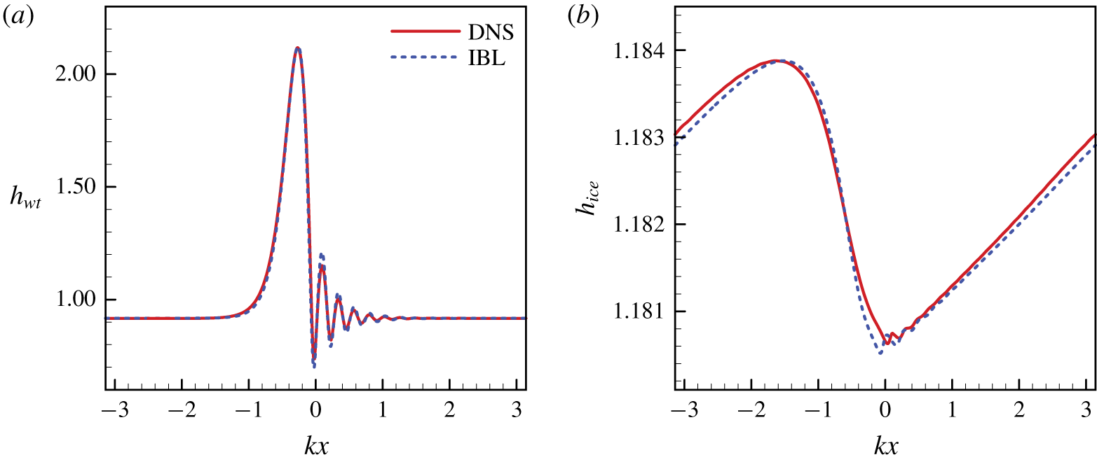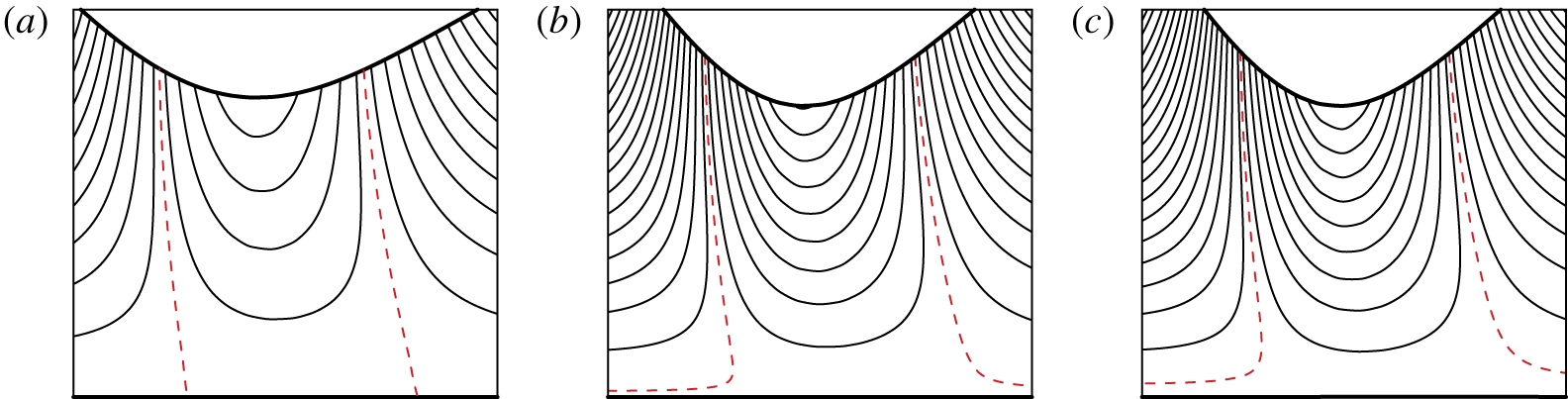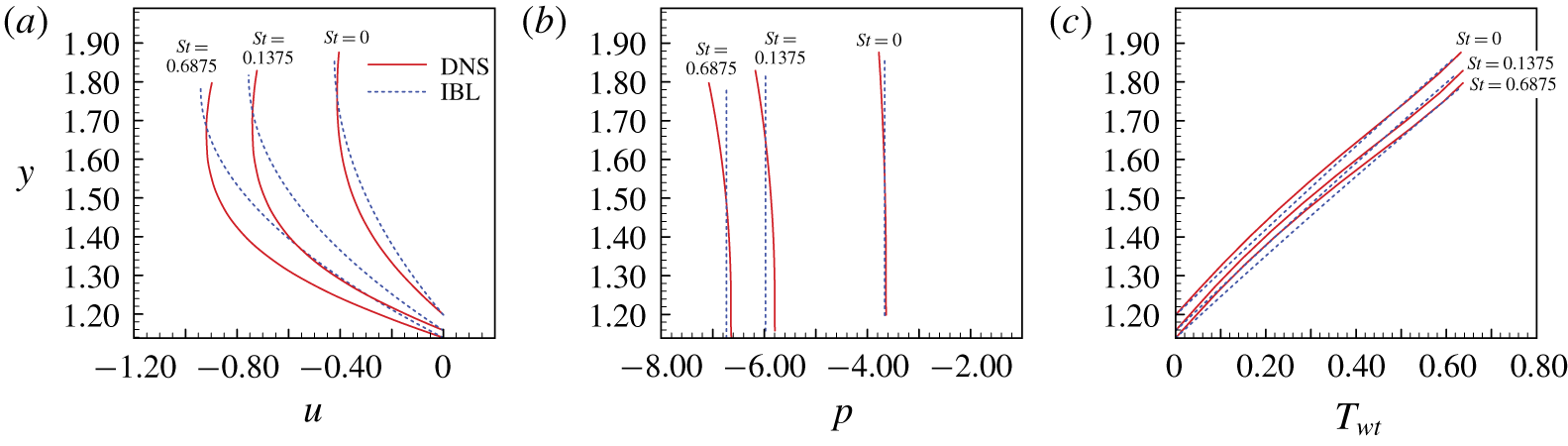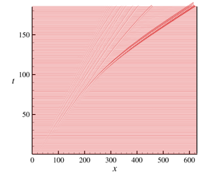
1 Introduction
The flow of a thin liquid film with a free surface has been the subject of intense investigation for several decades (Oron, Davis & Bankoff Reference Oron, Davis and Bankoff1997; Myers Reference Myers1998; Chang & Demekhin Reference Chang and Demekhin2002). Recently, a new level of complexity has been added to the problem by coupling the flow with a phase transition, which may include either evaporation/condensation (Burelbach, Bankoff & Davis Reference Burelbach, Bankoff and Davis1988; Aktershev & Alekseenko Reference Aktershev and Alekseenko2013) or solidification. For the latter circumstances, the hydrodynamics and morphological instabilities of the solidification interface, which could be attributed to the interaction between the unsteady solidification front and the flow of liquid phase, have been the subject of extensive research, for example, in the growth of large, single crystals for the fabrication of semiconductor wafers or in the casing of high-performance turbine blades for the aerospace industry (Yao & Prusa Reference Yao and Prusa1989; Davis Reference Davis2001). Besides, the effect of ice formation under a gravity-driven water film is of great practical importance in pipe freezing (Gilpin Reference Gilpin1981; Seki, Fukusako & Younan Reference Seki, Fukusako and Younan1984), airplane icing (Vargas & Reshotko Reference Vargas and Reshotko1998; Tsao & Rothmayer Reference Tsao and Rothmayer2000; Myers, Charpin & Thompson Reference Myers, Charpin and Thompson2002b; Moore, Mughal & Papageorgiou Reference Moore, Mughal and Papageorgiou2017) and shallow drainage conduits used in diverse engineering structures. In all these applications, the new feature we encountered is the interaction between an unsteady solidification front and the flow of the liquid phase. Since the phase transition requires the removal of heat, which can be carried by a flowing fluid, it has been appreciated that fluid dynamics play a significant role in the evolution of the solidification interface. At the same time, the development of the interface between a liquid and solid can respond to the flow characteristics. In many circumstances, the interface is unstable and prone to form corrugations (Worster, Batchelor & Moffatt Reference Worster, Batchelor and Moffatt2000). A characteristic instability feature on the solidification front has been observed (Forth & Wheeler Reference Forth and Wheeler1989). It is attributed to the upstream propagation of the solid/liquid interface disturbance, which depends on the length of the perturbation. Recently, an attempt to establish the formulation of ice growth on a flat substrate was presented within the context of airplane icing modelling (Myers, Charpin & Chapman Reference Myers, Charpin and Chapman2002a; Myers et al. Reference Myers, Charpin and Thompson2002b; Myers & Charpin Reference Myers and Charpin2004). The similar Stefan problems were conducted by using heat balance methods (Miladinova et al. Reference Miladinova, Slavtchev, Lebon and Legros2002; Mitchell & Myers Reference Mitchell and Myers2008, Reference Mitchell and Myers2012). The influence of an ice layer on the flow stability of a water film with a boundary-layer-scale was studied analytically by Timoshin (Reference Timoshin1997) and Tsao & Rothmayer (Reference Tsao and Rothmayer1998, Reference Tsao and Rothmayer2000, Reference Tsao and Rothmayer2002). For the super-cooled water in regimes with simultaneous air and water cooling, they found a new broadband ice instability mode, which can result in the formation of ice surface roughness on an airfoil leading edge during glaze ice accretion.
For water, the film flows on an inclined wall with the air temperature above freezing point, a steady-state solution of the Navier–Stokes and energy equations can be obtained, which makes it possible to perform a linear instability analysis consistently. Shapiro & Timoshin (Reference Shapiro and Timoshin2006, Reference Shapiro and Timoshin2007) considered the instability of a water-coated ice layer for the flow with large Reynolds and Froude numbers. A new mode of upstream-propagating instability was discovered, named the ice mode. It was explained according to the imbalance in heat flux caused by the small perturbation of the ice surface. Hu et al. (Reference Hu, Zhou, Hang, Liu and Zhang2010) studied the linear spatio-temporal instability of a falling water film along an inclined ice plane. The absolutely and convectively unstable regions are delineated. It was pointed out that the absolute instability did not appear either for the flow below a minimum Reynolds number or for the flow along the inclined ice plane above a maximum angle. Ueno & Farzaneh (Reference Ueno and Farzaneh2011) proposed a theoretical model for ice growth under a wind-driven super-cooled water film. The undisturbed solution was derived, and the linear instability analysis was carried out to study the morphological instability of the interface between the ice and water. They found the ice pattern of a centimetre-scale in wavelength, which decreases as the wind speed increases. More recently, Moore et al. (Reference Moore, Mughal and Papageorgiou2017) modelled the freezing of a thin film situated within an aerodynamic boundary layer due to the loss of heating on the part of a flat plate. According to the temperature difference across the ice, they divided the problem into two temporal regimes. A thorough asymptotic equation was derived and solved based on the incompressible Navier–Stokes equation.
In most practical cases, the film flow is unstable, and the liquid surface is covered by developing interfacial waves. It is well known that even in a laminar flow region, the presence of interfacial waves enhances the heat and mass transfer significantly, which may induce the temperature gradient along the liquid surface. As a result, the surface tension gradients (Marangoni effect) as a cause of interfacial instability (thermocapillary instability) can, in turn, affect the hydrodynamics of the liquid film. Joo, Davis & Bankoff (Reference Joo, Davis and Bankoff1991) investigated the thermocapillary instability of a thin liquid film falling down a uniformly heated inclined plane. Oron & Peles (Reference Oron and Peles1998) and Oron (Reference Oron, Shyy and Narayanan1999) examined the instability of a liquid film in the presence of a spatially uniform heat source within the liquid. Rednikov et al. (Reference Rednikov, Colinet, Velarde and Legros2000) considered the instability of a liquid layer resting on a flat horizontal rigid bottom. The liquid layer was heated either from below or above. They focused on the joint action of buoyancy and thermocapillary effects. It has been concluded that a film heated from above is a stabilizing setting. Kalliadasis, Kiyashko & Demekhin (Reference Kalliadasis, Kiyashko and Demekhin2003b) studied the instability of a thin liquid film heated by a local heat source. A set of the reduced equations for the Navier–Stokes/energy equations and free surface boundary conditions was derived based on the boundary layer approximation. More recently, Kalliadasis et al. (Reference Kalliadasis, Demekhin, Ruyer-Quil and Velarde2003a), Scheid et al. (Reference Scheid, Ruyer-Quil, Kalliadasis, Velarde and Zeytounian2005) and Ruyer-Quil et al. (Reference Ruyer-Quil, Scheid, Kalliadasis, Velarde and Zeytounian2005) revisited the dynamics of a thin liquid film falling along a uniform heated wall. The thermocapillary stress on the free surface caused by the surface tension gradients were considered. The results showed that thermocapillary stresses can affect the evolution of the film.
Although wave generation and transport processes in falling liquid films have been investigated extensively, and Chang & Demekhin (Reference Chang and Demekhin2002) has summarized the corresponding results, the literature for a systematic study on the wave dynamics in the film flow with a phase transition is currently scarce. No quantitative description can be found on the phase transport processes influences on the films nonlinear interfacial wave. Aktershev & Alekseenko (Reference Aktershev and Alekseenko2013) studied the nonlinear wave formation and heat transfer in wavy condensate film flowing over an isothermal wall by using the integral-boundary-layer (IBL) approximation. The evolution of both the natural waves arising due to the instability of the flow and the forced waves generated by small periodic perturbation of flow rate at the inlet was investigated. In this study, we consider the nonlinear hydrodynamics of a water film falling down an ice sheet. In particular, we focus on the flow with moderate Reynolds number. The purpose is to examine the nonlinear evolution of waves in the film with a solidification process. The interactions between the solidification front and the liquid flow coupling with the thermocapillary effect are our primary focus. Results of the reduced depth-averaged model are validated through comparisons to the direct numerical simulation (DNS) results. This, to our knowledge, has not been presented before.
The paper is organized as follows. The physical and numerical description of the problem is given in § 2. A coupled set of nonlinear evolution equations for the thickness of both the ice sheet and the water, the volumetric flow rate of the water film and the temperature gradients across the ice–water interface are presented. In § 3 the system is linearized with the instability characteristics being investigated by using the normal modes method. In § 4 the nonlinear solutions of steady travelling waves and spatio-temporal evolution of the system are discussed, which are compared to the direct numerical simulations in § 5. The conclusions are provided in § 6.
2 Problem formulation
2.1 Dimensionless governing equations
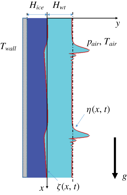
The geometry of a water film flowing down an ice sheet. The solid lines indicate the position of the ice–water interface and the air–water free surface. The initial equilibrium position of the unperturbed ice–water interface coincides with the  $x$-axis, and the dash–dot line denotes the initial equilibrium position of the unperturbed air–water free surface.

We consider a two-dimensional water film falling down a vertical ice sheet caused by gravity  $g$, as illustrated in figure 1. There are two layers: the water layer surrounded by the warm air, and the ice sheet rested on a cold solid wall. The temperature of the cold solid wall
 $T_{wall}$ is below the freezing point. The air–water interface is considered to be a free surface with a prescribed constant air pressure
 $p_{air}$ and temperature
 $T_{air}$ above the freezing point. The temperature of the air–water interface, which is not constrained to be constant, is determined according to Newton’s law of cooling. The effect of buoyancy is neglected since the thickness of the water film is assumed to be very small. A cartesian coordinate system (
 $x,y$) is introduced to model the two-dimensional film dynamics. The
 $x$-axis orients downwards along with the unperturbed ice–water interface, and the
 $y$-axis denotes the corresponding normal direction. The liquid water with density
 $\unicode[STIX]{x1D70C}_{wt}$ and viscosity
 $\unicode[STIX]{x1D707}_{wt}$ occupies the region
 $\unicode[STIX]{x1D701}(x,t)\leqslant y\leqslant \unicode[STIX]{x1D702}(x,t)$, where
 $\unicode[STIX]{x1D701}(x,t)$ and
 $\unicode[STIX]{x1D702}(x,t)$ indicate the perturbed position of the air–water free surface and the ice–water interface. The pressure and film velocity components along the
 $x$ and
 $y$ directions are denoted by
 $p$,
 $u$ and
 $v$, respectively.
For the system under consideration, the water film is assumed to be very thin. The time scales of the film dynamics and the heat transfer behaviour are of the same order (Miladinova et al. Reference Miladinova, Slavtchev, Lebon and Legros2002). Therefore, the problem is considered on the time scale of the evolution of the water film. The dynamic characteristics of the water film are of primary concern. For the sake of brevity, we present the model in the dimensionless form directly and use the following scales:
 $$\begin{eqnarray}\displaystyle & \displaystyle (x,y)=\left(\frac{x^{\ast }}{\unicode[STIX]{x1D700}},y^{\ast }\right)H_{wt},\quad (u,v)=(u^{\ast },\unicode[STIX]{x1D700}v^{\ast })u_{s},\quad p=\unicode[STIX]{x1D70C}_{wt}u_{s}^{2}p^{\ast },\quad t=t^{\ast }\frac{H_{wt}}{\unicode[STIX]{x1D700}u_{s}}, & \displaystyle \nonumber\\ \displaystyle & \displaystyle (\unicode[STIX]{x1D702},\unicode[STIX]{x1D701})=(\unicode[STIX]{x1D702}^{\ast },\unicode[STIX]{x1D701}^{\ast })H_{wt},\quad T=T_{fr}+T^{\ast }\unicode[STIX]{x0394}T. & \displaystyle \nonumber\end{eqnarray}$$
Here  $\unicode[STIX]{x1D700}=H_{wt}/L$,
 $H_{wt}$ is the thickness for the unperturbed water film,
 $L$ represents the wavelength of a typical deformation of the air–water free surface,
 $u_{s}=\unicode[STIX]{x1D70C}_{wt}gH_{wt}^{2}/(2\unicode[STIX]{x1D707}_{wt})$ is the Nusselt surface velocity of an unperturbed water film (Nusselt Reference Nusselt1923),
 $T_{fr}$ is the freezing temperature of the water and
 $\unicode[STIX]{x0394}T=T_{air}-T_{wall}$ denotes the temperature difference between the warm air and the cold solid wall. Hereafter, the superscripts ‘
 $\ast$’, which denote the dimensionless quantities, are suppressed for the purpose of brevity. The dimensionless governing equations of motion can be written as (Miladinova et al. Reference Miladinova, Slavtchev, Lebon and Legros2002; Dietze, Leefken & Kneer Reference Dietze, Leefken and Kneer2008)
 $$\begin{eqnarray}\displaystyle & \displaystyle \frac{\unicode[STIX]{x2202}u}{\unicode[STIX]{x2202}x}+\frac{\unicode[STIX]{x2202}v}{\unicode[STIX]{x2202}y}=0, & \displaystyle\end{eqnarray}$$
 $$\begin{eqnarray}\displaystyle & \displaystyle \frac{\unicode[STIX]{x2202}u}{\unicode[STIX]{x2202}t}+u\frac{\unicode[STIX]{x2202}u}{\unicode[STIX]{x2202}x}+v\frac{\unicode[STIX]{x2202}u}{\unicode[STIX]{x2202}y}=-\frac{\unicode[STIX]{x2202}p}{\unicode[STIX]{x2202}x}+\frac{1}{\unicode[STIX]{x1D700}Re}\left(\unicode[STIX]{x1D700}^{2}\frac{\unicode[STIX]{x2202}^{2}u}{\unicode[STIX]{x2202}x^{2}}+\frac{\unicode[STIX]{x2202}^{2}u}{\unicode[STIX]{x2202}y^{2}}\right)+\frac{2}{\unicode[STIX]{x1D700}Re}, & \displaystyle\end{eqnarray}$$
 $$\begin{eqnarray}\displaystyle & \displaystyle \frac{\unicode[STIX]{x2202}v}{\unicode[STIX]{x2202}t}+u\frac{\unicode[STIX]{x2202}v}{\unicode[STIX]{x2202}x}+v\frac{\unicode[STIX]{x2202}v}{\unicode[STIX]{x2202}y}=-\frac{1}{\unicode[STIX]{x1D700}^{2}}\frac{\unicode[STIX]{x2202}p}{\unicode[STIX]{x2202}y}+\frac{1}{\unicode[STIX]{x1D700}Re}\left(\unicode[STIX]{x1D700}^{2}\frac{\unicode[STIX]{x2202}^{2}v}{\unicode[STIX]{x2202}x^{2}}+\frac{\unicode[STIX]{x2202}^{2}v}{\unicode[STIX]{x2202}y^{2}}\right). & \displaystyle\end{eqnarray}$$
Here,  $Re=\unicode[STIX]{x1D70C}_{wt}u_{s}H_{wt}/\unicode[STIX]{x1D707}_{wt}=2u_{s}^{2}/(gH_{wt})$ is the Reynolds number. For the energy equation of water film, we have
 $$\begin{eqnarray}\frac{\unicode[STIX]{x2202}T_{wt}}{\unicode[STIX]{x2202}t}+u\frac{\unicode[STIX]{x2202}T_{wt}}{\unicode[STIX]{x2202}x}+v\frac{\unicode[STIX]{x2202}T_{wt}}{\unicode[STIX]{x2202}y}=\frac{1}{\unicode[STIX]{x1D700}RePr}\left(\unicode[STIX]{x1D700}^{2}\frac{\unicode[STIX]{x2202}^{2}T_{wt}}{\unicode[STIX]{x2202}x^{2}}+\frac{\unicode[STIX]{x2202}^{2}T_{wt}}{\unicode[STIX]{x2202}y^{2}}\right),\end{eqnarray}$$
where the dissipation caused by the viscous stresses is ignored. We denote by  $T_{wt}$ the temperature distribution in the water film,
 $Pr=\unicode[STIX]{x1D707}_{wt}/(\unicode[STIX]{x1D70C}_{wt}K_{wt})$ is the Prandtl number and
 $K_{wt}$ is the thermal diffusivity of liquid water. The dimensionless energy equation of the ice sheet can be expressed as
 $$\begin{eqnarray}\frac{\unicode[STIX]{x2202}T_{ice}}{\unicode[STIX]{x2202}t}=\frac{\unicode[STIX]{x1D6FC}}{\unicode[STIX]{x1D700}RePr}\left(\unicode[STIX]{x1D700}^{2}\frac{\unicode[STIX]{x2202}^{2}T_{ice}}{\unicode[STIX]{x2202}x^{2}}+\frac{\unicode[STIX]{x2202}^{2}T_{ice}}{\unicode[STIX]{x2202}y^{2}}\right).\end{eqnarray}$$
Here  $T_{ice}$ is the temperature distribution in the ice sheet and
 $\unicode[STIX]{x1D6FC}=K_{ice}/K_{wt}$ denotes the ratio of thermal diffusivity between the ice sheet and the water film. The dimensionless boundary conditions associated with the above governing equations are as follows.
(i) The boundary conditions at the air–water free surface  $y=\unicode[STIX]{x1D702}(x,t)$ include the balance of tangential and normal stresses at the surface:
 $$\begin{eqnarray}\frac{2\unicode[STIX]{x1D700}^{2}\unicode[STIX]{x1D702}_{x}}{Re}\left(\frac{\unicode[STIX]{x2202}v}{\unicode[STIX]{x2202}y}-\frac{\unicode[STIX]{x2202}u}{\unicode[STIX]{x2202}x}\right)+\frac{(1-\unicode[STIX]{x1D700}^{2}\unicode[STIX]{x1D702}_{x}^{2})}{Re}\left(\unicode[STIX]{x1D700}^{2}\frac{\unicode[STIX]{x2202}v}{\unicode[STIX]{x2202}x}+\frac{\unicode[STIX]{x2202}u}{\unicode[STIX]{x2202}y}\right)=\sqrt{1+\unicode[STIX]{x1D700}^{2}\unicode[STIX]{x1D702}_{x}^{2}}\frac{\unicode[STIX]{x1D700}}{We}\frac{\unicode[STIX]{x2202}\unicode[STIX]{x1D70E}}{\unicode[STIX]{x2202}x},\end{eqnarray}$$
 $$\begin{eqnarray}(1+\unicode[STIX]{x1D700}^{2}\unicode[STIX]{x1D702}_{x}^{2})(p-p_{air})-2\frac{\unicode[STIX]{x1D700}}{Re}\frac{\unicode[STIX]{x2202}v}{\unicode[STIX]{x2202}y}+2\frac{\unicode[STIX]{x1D700}\unicode[STIX]{x1D702}_{x}}{Re}\left(\unicode[STIX]{x1D700}^{2}\frac{\unicode[STIX]{x2202}v}{\unicode[STIX]{x2202}x}+\frac{\unicode[STIX]{x2202}u}{\unicode[STIX]{x2202}y}\right)-2\frac{\unicode[STIX]{x1D700}^{3}\unicode[STIX]{x1D702}_{x}^{2}}{Re}\frac{\unicode[STIX]{x2202}u}{\unicode[STIX]{x2202}x}=-\unicode[STIX]{x1D700}^{2}\frac{\unicode[STIX]{x1D702}_{xx}\unicode[STIX]{x1D70E}}{\sqrt{1+\unicode[STIX]{x1D700}^{2}\unicode[STIX]{x1D702}_{x}^{2}}We}.\end{eqnarray}$$
Here,  $\unicode[STIX]{x1D702}_{x}=\unicode[STIX]{x2202}\unicode[STIX]{x1D702}/\unicode[STIX]{x2202}x$,
 $We=\unicode[STIX]{x1D70C}_{wt}u_{s}^{2}H_{wt}/\unicode[STIX]{x1D70E}_{0}$ is defined as the Weber number and, for the sake of simplicity, the prescribed pressure of the outside air
 $p_{air}$ is assumed to be zero. The variation of surface tension with temperature (thermocapillary effect) is modelled by the linear approximation (Ruyer-Quil et al. Reference Ruyer-Quil, Scheid, Kalliadasis, Velarde and Zeytounian2005)
 $$\begin{eqnarray}\unicode[STIX]{x1D70E}=1-M(T-T_{0}),\end{eqnarray}$$
where  $M=-\unicode[STIX]{x0394}T(\text{d}\unicode[STIX]{x1D70E}/\text{d}T)_{T_{0}}/\unicode[STIX]{x1D70E}_{0}$ is defined as the Marangoni number and
 $T_{0}$ is the reference temperature with corresponding surface tension
 $\unicode[STIX]{x1D70E}_{0}$. It can be either the interfacial temperature of the basic state, i.e. the tranquil uniform film or the air temperature. In this study,
 $T_{0}$ is defined as the interfacial temperature of the basic state. The kinematic condition at the free surface is given as
 $$\begin{eqnarray}\frac{\unicode[STIX]{x2202}\unicode[STIX]{x1D702}}{\unicode[STIX]{x2202}t}+\unicode[STIX]{x1D702}_{x}u-v=0.\end{eqnarray}$$
Applying Newton’s law of cooling at the air–water free surface gives
 $$\begin{eqnarray}\left(\frac{\unicode[STIX]{x2202}T_{wt}}{\unicode[STIX]{x2202}y}-\unicode[STIX]{x1D700}^{2}\unicode[STIX]{x1D702}_{x}\frac{\unicode[STIX]{x2202}T_{wt}}{\unicode[STIX]{x2202}x}\right)+Bi\sqrt{1+\unicode[STIX]{x1D700}^{2}\unicode[STIX]{x1D702}_{x}^{2}}(T_{wt}-T_{air})=0.\end{eqnarray}$$
The Biot number is defined as  $Bi=\unicode[STIX]{x1D717}H_{wt}/\unicode[STIX]{x1D706}_{wt}$, where
 $\unicode[STIX]{x1D706}_{wt}=K_{wt}\unicode[STIX]{x1D70C}_{wt}C_{wt}$ is the thermal conductivity of the liquid water,
 $\unicode[STIX]{x1D717}$ is the heat transfer coefficient and
 $C_{wt}$ is the constant-pressure heat capacity.
(ii) The boundary conditions at the ice–water interface  $y=\unicode[STIX]{x1D701}(x,t)$ are given as (Worster et al. Reference Worster, Batchelor and Moffatt2000; Hu et al. Reference Hu, Zhou, Hang, Liu and Zhang2010; Moore et al. Reference Moore, Mughal and Papageorgiou2017)
 $$\begin{eqnarray}\displaystyle & \displaystyle \unicode[STIX]{x1D712}\frac{\unicode[STIX]{x2202}\unicode[STIX]{x1D701}}{\unicode[STIX]{x2202}t}+\unicode[STIX]{x1D701}_{x}u-v=0, & \displaystyle\end{eqnarray}$$
 $$\begin{eqnarray}\displaystyle & \displaystyle \frac{\unicode[STIX]{x1D700}}{\unicode[STIX]{x1D712}}\frac{RePr}{St}(v-\unicode[STIX]{x1D701}_{x}u)=\left(\unicode[STIX]{x1D6FD}\frac{\unicode[STIX]{x2202}T_{ice}}{\unicode[STIX]{x2202}y}-\frac{\unicode[STIX]{x2202}T_{wt}}{\unicode[STIX]{x2202}y}\right)-\unicode[STIX]{x1D700}^{2}\unicode[STIX]{x1D701}_{x}\left(\unicode[STIX]{x1D6FD}\frac{\unicode[STIX]{x2202}T_{ice}}{\unicode[STIX]{x2202}x}-\frac{\unicode[STIX]{x2202}T_{wt}}{\unicode[STIX]{x2202}x}\right), & \displaystyle\end{eqnarray}$$
 $$\begin{eqnarray}\displaystyle & \displaystyle T_{ice}=T_{wt}=T_{fr}=0. & \displaystyle\end{eqnarray}$$
Here,  $\unicode[STIX]{x1D701}_{x}=\unicode[STIX]{x2202}\unicode[STIX]{x1D701}/\unicode[STIX]{x2202}x$ and
 $\unicode[STIX]{x1D712}=1-\unicode[STIX]{x1D70C}_{ice}/\unicode[STIX]{x1D70C}_{wt}$, where
 $\unicode[STIX]{x1D70C}_{ice}$ indicates the density of ice. Equation (2.11) shows the kinematic condition for the ice–water interface and describes its evolution. Here
 $\unicode[STIX]{x1D712}$ accounts for the influence of density differences between the ice and water (Lock et al. Reference Lock and Lock1990). Equation (2.12) stands for the conservation of heat flux at the ice–water interface, which is usually known as the Stefan condition (Meirmanov Reference Meirmanov2011; Alexiades Reference Alexiades2017). It means that the release of latent heat at the ice–water interface is balanced by the net heat flux away from the interface. The complete form of (2.12) can be deduced from the conservation equations of mass, momentum and energy (Lin & Hudman Reference Lin and Hudman1996) at the ice–water interface. Here
 $\unicode[STIX]{x1D6FD}=\unicode[STIX]{x1D706}_{ice}/\unicode[STIX]{x1D706}_{wt}$ is the ratio of thermal conductivities between the ice and water. We define the Stefan number
 $St$ as
 $$\begin{eqnarray}St=\frac{\unicode[STIX]{x1D70C}_{wt}C_{wt}\unicode[STIX]{x0394}T}{\unicode[STIX]{x1D70C}_{ice}Q_{lh}},\end{eqnarray}$$
where  $Q_{lh}$ is the latent heat, which is defined by the amount of heat required to change a unit mass of solid ice into liquid water at the freezing temperature. It is worth noting that the evolution of the ice surface is linked to the flow field via the Stefan condition (Alexiades Reference Alexiades2017). It has been observed in numerical computation that, for water near
 $0\,^{\circ }\text{C}$, the time required for the ice structure to reach a final steady-state in a temporal evolution is inversely proportional to the Stefan number
 $St$ (Lee Reference Lee1993). Shapiro & Timoshin (Reference Shapiro and Timoshin2007) claimed that the time derivatives in the governing equations can be neglected for the flow with a small Stefan number
 $St$. The flow of water can be treated as quasi-steady. However, in this study, we consider the problem on the time scale of the evolution of the water film. The interaction between the unsteady flow field and the development of ice-sheet topography can be revealed. Since the water is pure and there is no mushy layer (see Feltham & Worster (Reference Feltham and Worster1999) instead), the zero tangential velocity condition at the ice–water interface can be expressed as (Forth & Wheeler Reference Forth and Wheeler1989; Ueno & Farzaneh Reference Ueno and Farzaneh2011)
 $$\begin{eqnarray}u+\unicode[STIX]{x1D700}^{2}\unicode[STIX]{x1D701}_{x}v=0.\end{eqnarray}$$
(iii) The temperature boundary condition at the cold solid wall  $(y=-\unicode[STIX]{x1D6FF})$ is
 $$\begin{eqnarray}T_{ice}=T_{wall},\end{eqnarray}$$
where  $\unicode[STIX]{x1D6FF}=H_{ice}/H_{wt}$ denotes the dimensionless thickness of the ice sheet. Here, similar to the flow considered in previous literature (Shapiro & Timoshin Reference Shapiro and Timoshin2006, Reference Shapiro and Timoshin2007; Hu et al. Reference Hu, Zhou, Hang, Liu and Zhang2010), we derive the basic state (steady Nusselt flow) solution of the water film and ice sheet to perform the linear instability analysis. According to the above equations (2.1)–(2.15), we have
 $$\begin{eqnarray}\left.\begin{array}{@{}c@{}}u_{0}=y(2-y),\quad v_{0}=0,\quad p_{0}=0,\\ \unicode[STIX]{x1D702}_{0}=1,\quad \unicode[STIX]{x1D701}_{0}=0,\\ T_{wt,0}=T_{air}{\displaystyle \frac{Bi}{1+Bi}}y,\quad T_{ice,0}=T_{air}{\displaystyle \frac{Bi}{\unicode[STIX]{x1D6FD}(1+Bi)}}y.\end{array}\right\}\end{eqnarray}$$
Since we have  $T_{air}-T_{wall}=1$, the expression of ice sheet thickness
 $\unicode[STIX]{x1D6FF}$ can be given as
 $$\begin{eqnarray}\displaystyle \unicode[STIX]{x1D6FF}=\unicode[STIX]{x1D6FD}\left(1+\frac{1}{Bi}\right)\frac{1-T_{air}}{T_{air}}. & & \displaystyle\end{eqnarray}$$
Here, the thickness of the tranquil uniform ice-sheet  $\unicode[STIX]{x1D6FF}$ depends on the air temperature
 $T_{air}$, the ratio of thermal conductivities
 $\unicode[STIX]{x1D6FD}$ and the Biot number
 $Bi$. This indicates that the system is in a thermal equilibrium state, and the phase transition between the ice and water is balanced. The thickness of the ice sheet is constant along the downstream. However, when the transient state is considered, the thermal equilibrium cannot be achieved. The phase transition occurs at the ice–water interface, and the topography of the ice-sheet changes spatio-temporally.
2.2 Scaling
The above-stated equations (2.1)–(2.15) can exactly describe the nonlinear evolution of the system and, in general, require an arduous numerical simulation, as shown in § 5. To alleviate this difficulty, we try to model the dynamics of long interfacial waves by using the IBL approximation. The starting point is to assume long waves in the  $x$-direction. Then, we have
 $\unicode[STIX]{x1D700}=H_{wt}/L\ll 1$, and the reduced governing equations for the leading order in
 $\unicode[STIX]{x1D700}$ shown to be
 $$\begin{eqnarray}\displaystyle & \displaystyle \frac{\unicode[STIX]{x2202}u}{\unicode[STIX]{x2202}x}+\frac{\unicode[STIX]{x2202}v}{\unicode[STIX]{x2202}y}=0, & \displaystyle\end{eqnarray}$$
 $$\begin{eqnarray}\displaystyle & \displaystyle \frac{\unicode[STIX]{x2202}u}{\unicode[STIX]{x2202}t}+u\frac{\unicode[STIX]{x2202}u}{\unicode[STIX]{x2202}x}+v\frac{\unicode[STIX]{x2202}u}{\unicode[STIX]{x2202}y}=-\frac{\unicode[STIX]{x2202}p}{\unicode[STIX]{x2202}x}+\frac{1}{\unicode[STIX]{x1D700}Re}\frac{\unicode[STIX]{x2202}^{2}u}{\unicode[STIX]{x2202}y^{2}}+\frac{2}{\unicode[STIX]{x1D700}Re}, & \displaystyle\end{eqnarray}$$
 $$\begin{eqnarray}\displaystyle & \displaystyle \frac{\unicode[STIX]{x2202}p}{\unicode[STIX]{x2202}y}=0, & \displaystyle\end{eqnarray}$$
 $$\begin{eqnarray}\displaystyle & \displaystyle \frac{\unicode[STIX]{x2202}T_{wt}}{\unicode[STIX]{x2202}t}+u\frac{\unicode[STIX]{x2202}T_{wt}}{\unicode[STIX]{x2202}x}+v\frac{\unicode[STIX]{x2202}T_{wt}}{\unicode[STIX]{x2202}y}=\frac{1}{\unicode[STIX]{x1D700}RePr}\frac{\unicode[STIX]{x2202}^{2}T_{wt}}{\unicode[STIX]{x2202}y^{2}}, & \displaystyle\end{eqnarray}$$
 $$\begin{eqnarray}\displaystyle & \displaystyle \frac{\unicode[STIX]{x2202}T_{ice}}{\unicode[STIX]{x2202}t}=\frac{\unicode[STIX]{x1D6FC}}{\unicode[STIX]{x1D700}RePr}\frac{\unicode[STIX]{x2202}^{2}T_{ice}}{\unicode[STIX]{x2202}y^{2}}. & \displaystyle\end{eqnarray}$$
The boundary conditions on the ice–water interface  $y=\unicode[STIX]{x1D701}(x,t)$ can be reduced to
 $$\begin{eqnarray}u=0,\quad v=\unicode[STIX]{x1D712}\frac{\unicode[STIX]{x2202}\unicode[STIX]{x1D701}}{\unicode[STIX]{x2202}t},\end{eqnarray}$$
 $$\begin{eqnarray}\displaystyle \frac{\unicode[STIX]{x1D700}}{\unicode[STIX]{x1D712}}\frac{RePr}{St}v=\unicode[STIX]{x1D6FD}\frac{\unicode[STIX]{x2202}T_{ice}}{\unicode[STIX]{x2202}y}-\frac{\unicode[STIX]{x2202}T_{wt}}{\unicode[STIX]{x2202}y}, & & \displaystyle\end{eqnarray}$$
 $$\begin{eqnarray}\displaystyle T_{ice}=T_{wt}=T_{fr}=0. & & \displaystyle\end{eqnarray}$$
The corresponding boundary conditions on the air–water free surface  $y=\unicode[STIX]{x1D702}(x,t)$ are
 $$\begin{eqnarray}\displaystyle & \displaystyle \frac{\unicode[STIX]{x2202}u}{\unicode[STIX]{x2202}y}=-\unicode[STIX]{x1D700}\frac{Re}{We}M\frac{\unicode[STIX]{x2202}T_{wt}}{\unicode[STIX]{x2202}x}, & \displaystyle\end{eqnarray}$$
 $$\begin{eqnarray}\displaystyle & \displaystyle p=-\frac{\unicode[STIX]{x1D700}^{2}}{We}\unicode[STIX]{x1D702}_{xx}, & \displaystyle\end{eqnarray}$$
 $$\begin{eqnarray}\displaystyle & \displaystyle \frac{\unicode[STIX]{x2202}\unicode[STIX]{x1D702}}{\unicode[STIX]{x2202}t}+u\frac{\unicode[STIX]{x2202}\unicode[STIX]{x1D702}}{\unicode[STIX]{x2202}x}-v=0, & \displaystyle\end{eqnarray}$$
 $$\begin{eqnarray}\displaystyle & \displaystyle \frac{\unicode[STIX]{x2202}T_{wt}}{\unicode[STIX]{x2202}y}+Bi(T_{wt}-T_{air})=0. & \displaystyle\end{eqnarray}$$
The expression of the temperature boundary condition on the solid wall ( $y=-\unicode[STIX]{x1D6FF}$) is the same as (2.15). From the above equations, we know that for a long-wave approximation, the system hydrodynamics can be characterized by the following dimensionless parameters:
 $$\begin{eqnarray}T_{air},\quad Re,\quad We,\quad M,\quad Bi,\quad St,\quad Pr,\quad \unicode[STIX]{x1D6FC},\quad \unicode[STIX]{x1D6FD},\quad \unicode[STIX]{x1D712},\quad \unicode[STIX]{x1D700}.\end{eqnarray}$$
Physically, for the falling film, the most interesting case is when the viscous, gravitational, capillary/thermocapillary terms are of the same order. Thus, we rescale the dimensionless parameters  $Re$,
 $We$,
 $M$ as follows (Matar, Craster & Kumar Reference Matar, Craster and Kumar2007; Sisoev et al. Reference Sisoev, Matar, Craster and Kumar2010; Peng, Zhang & Zhuge Reference Peng, Zhang and Zhuge2014):
 $$\begin{eqnarray}Re_{\unicode[STIX]{x1D700}}=\unicode[STIX]{x1D700}Re,\quad We_{\unicode[STIX]{x1D700}}=We/\unicode[STIX]{x1D700}^{2},\quad M_{\unicode[STIX]{x1D700}}=M/\unicode[STIX]{x1D700}^{2}.\end{eqnarray}$$
Since the flow with moderate Reynolds number is considered, in this study we can assume that  $Re=O(\unicode[STIX]{x1D700}^{-1})$. For the corresponding dimensionless parameters with the same order, hereinafter, we have
 $(Re_{\unicode[STIX]{x1D700}},We_{\unicode[STIX]{x1D700}},M_{\unicode[STIX]{x1D700}})=O(1)$.
2.3 Integral-boundary-layer equations for moderate Reynolds number
According to the IBL theory, we integrate the above reduced Navier–Stokes/energy equations across the thickness of the water film and the ice sheet. The profiles of the velocity and temperature are needed to close the problem (Ruyer-Quil et al. Reference Ruyer-Quil, Scheid, Kalliadasis, Velarde and Zeytounian2005; Peng et al. Reference Peng, Jiang, Zhuge and Zhang2016). According to the boundary condition (2.26), in the presence of Marangoni stress, the most straightforward possible profile of the velocity can be assumed to be
 $$\begin{eqnarray}u=-\frac{3q}{2(\unicode[STIX]{x1D702}-\unicode[STIX]{x1D701})^{3}}(y-\unicode[STIX]{x1D701})(y+\unicode[STIX]{x1D701}-2\unicode[STIX]{x1D702})-M_{a}\unicode[STIX]{x1D713}\frac{(y-\unicode[STIX]{x1D701})(3y-\unicode[STIX]{x1D701}-2\unicode[STIX]{x1D702})}{4(\unicode[STIX]{x1D702}-\unicode[STIX]{x1D701})}.\end{eqnarray}$$
Here,  $M_{a}=M_{\unicode[STIX]{x1D700}}Re_{\unicode[STIX]{x1D700}}/We_{\unicode[STIX]{x1D700}}=O(1)$ and
 $\unicode[STIX]{x1D713}=(\unicode[STIX]{x2202}T_{wt}/\unicode[STIX]{x2202}x)_{\unicode[STIX]{x1D702}}$ is the temperature gradient on the air–water free surface along the
 $x$-direction. It can be derived from the temperature profile in the water film. According to the second term on the right-hand side of (2.31), the boundary condition (2.26) is satisfied automatically. For the temperature distribution across the water film and the ice sheet, we assume that the profiles are as follows:
 $$\begin{eqnarray}\displaystyle & \displaystyle T_{wt}=\frac{Bi(T_{air}-g_{wt}(\unicode[STIX]{x1D702}-\unicode[STIX]{x1D701}))-g_{wt}}{Bi(\unicode[STIX]{x1D702}-\unicode[STIX]{x1D701})^{2}+2(\unicode[STIX]{x1D702}-\unicode[STIX]{x1D701})}(y-\unicode[STIX]{x1D701})^{2}+g_{wt}(y-\unicode[STIX]{x1D701}), & \displaystyle\end{eqnarray}$$
 $$\begin{eqnarray}\displaystyle & \displaystyle T_{ice}=T_{wall}\left(\frac{y-\unicode[STIX]{x1D701}}{\unicode[STIX]{x1D6FF}+\unicode[STIX]{x1D701}}\right)^{2}+\frac{g_{ice}}{(\unicode[STIX]{x1D6FF}+\unicode[STIX]{x1D701})}(y+\unicode[STIX]{x1D6FF})(y-\unicode[STIX]{x1D701}). & \displaystyle\end{eqnarray}$$
Here,  $T_{wall}=T_{air}-1$. The temperature boundary conditions on the cold solid wall, ice–water interface and the air–water free surface, which are denoted by (2.15), (2.25) and (2.29), are satisfied precisely. According to (2.32) and (2.33), the parameters
 $g_{wt}$ and
 $g_{ice}$ are defined as
 $$\begin{eqnarray}g_{ice}=\left.\frac{\unicode[STIX]{x2202}T_{ice}}{\unicode[STIX]{x2202}y}\right|_{\unicode[STIX]{x1D701}},\quad g_{wt}=\left.\frac{\unicode[STIX]{x2202}T_{wt}}{\unicode[STIX]{x2202}y}\right|_{\unicode[STIX]{x1D701}},\end{eqnarray}$$
which are the temperature gradients on both sides of the ice–water interface along the  $y$-direction, respectively. When the steady Nusselt flow is considered, (2.32) and (2.33) can be reduced to the linear profiles, as shown in (2.16). Thus, we believe that (2.32) and (2.33) are improved compared to the linear profiles presented in previous literature (Kalliadasis et al. Reference Kalliadasis, Kiyashko and Demekhin2003b; Shapiro & Timoshin Reference Shapiro and Timoshin2007), where a linear temperature profile is adopted, and Newton’s law of cooling at the air–water free surface is satisfied on average. Here, we choose to emphasize the temperature gradients
 $g_{wt}$ and
 $g_{ice}$ because they appear directly in the boundary condition (2.24) and the temperature profiles. Thus, they have an essential influence on the movement of the ice–water interface. According to (2.32), the expression of the temperature gradient along the
 $x$-direction on the air–water free surface included in (2.31) is
 $$\begin{eqnarray}\displaystyle \unicode[STIX]{x1D713}=\left.\frac{\unicode[STIX]{x2202}T_{wt}}{\unicode[STIX]{x2202}x}\right|_{\unicode[STIX]{x1D702}}=2\frac{g_{wt}+BiT_{air}}{(2+Bih_{wt})^{2}}\frac{\unicode[STIX]{x2202}h_{wt}}{\unicode[STIX]{x2202}x}+\frac{h_{wt}}{2+Bih_{wt}}\frac{\unicode[STIX]{x2202}g_{wt}}{\unicode[STIX]{x2202}x}. & & \displaystyle\end{eqnarray}$$
Here,  $h_{wt}=\unicode[STIX]{x1D702}-\unicode[STIX]{x1D701}$ represents the thickness of the water film. Integrating (2.19) along with the film thickness, and considering the continuity equation (2.18), Leibnitz rule, the boundary conditions (2.23) at the ice–water interface, the kinematic conditions (2.28) at the air–water surface and the velocity profile (2.31) leads to the integral form of the momentum equation
 $$\begin{eqnarray}\displaystyle \frac{\unicode[STIX]{x2202}q}{\unicode[STIX]{x2202}t} & = & \displaystyle \frac{h_{wt}}{We_{\unicode[STIX]{x1D700}}}\frac{\unicode[STIX]{x2202}^{3}(h_{ice}+h_{wt})}{\unicode[STIX]{x2202}x^{3}}+\frac{1}{Re_{\unicode[STIX]{x1D700}}}\left(2h_{wt}-\frac{3q}{h_{wt}^{2}}\right)-\frac{6}{5}\frac{\unicode[STIX]{x2202}}{\unicode[STIX]{x2202}x}\left(\frac{q^{2}}{h_{wt}}\right)\nonumber\\ \displaystyle & & \displaystyle -\,\frac{3}{2}\frac{M_{a}}{Re_{\unicode[STIX]{x1D700}}}\unicode[STIX]{x1D713}-\frac{\unicode[STIX]{x2202}}{\unicode[STIX]{x2202}x}\left(\frac{M_{a}^{2}}{120}\unicode[STIX]{x1D713}^{2}h_{wt}^{3}-\frac{M_{a}}{20}q\unicode[STIX]{x1D713}h_{wt}\right).\end{eqnarray}$$
Here,  $q=\int _{\unicode[STIX]{x1D701}}^{\unicode[STIX]{x1D702}}u\,\text{d}y$ is the flow rate of the water film. The continuity equation (2.18) can be reduced to
 $$\begin{eqnarray}\frac{\unicode[STIX]{x2202}h_{wt}}{\unicode[STIX]{x2202}t}+(1-\unicode[STIX]{x1D712})\frac{\unicode[STIX]{x2202}h_{ice}}{\unicode[STIX]{x2202}t}+\frac{\unicode[STIX]{x2202}q}{\unicode[STIX]{x2202}x}=0.\end{eqnarray}$$
Combining with the velocity and temperature profile equations (2.31) and (2.32), the final averaged energy equation in the water film can be obtained by integrating (2.21) along with the thickness of the water film. Thus, we have
 $$\begin{eqnarray}\displaystyle \frac{\unicode[STIX]{x2202}g_{wt}}{\unicode[STIX]{x2202}t} & = & \displaystyle \frac{12}{Re_{\unicode[STIX]{x1D700}}Pr}\left(\frac{Bi(T_{air}-g_{wt}h_{wt})-g_{wt}}{(4+Bih_{wt})h_{wt}^{2}}\right)-\frac{3}{20}\frac{(32+7Bih_{wt})}{(4+Bih_{wt})}\frac{q}{h_{wt}}\frac{\unicode[STIX]{x2202}g_{wt}}{\unicode[STIX]{x2202}x}\nonumber\\ \displaystyle & & \displaystyle -\,2\frac{g_{wt}(8+5Bih_{wt}+Bi^{2}h_{wt}^{2})+Bi(4+Bih_{wt})T_{air}}{(2+Bih_{wt})(4+Bih_{wt})h_{wt}}\frac{\unicode[STIX]{x2202}h_{wt}}{\unicode[STIX]{x2202}t}\nonumber\\ \displaystyle & & \displaystyle -\,\frac{3}{20}\frac{g_{wt}(64+28Bih_{wt}+7Bi^{2}h_{wt}^{2})+36BiT_{air}}{(2+Bih_{wt})(4+Bih_{wt})}\frac{q}{h_{wt}^{2}}\frac{\unicode[STIX]{x2202}h_{wt}}{\unicode[STIX]{x2202}x}\nonumber\\ \displaystyle & & \displaystyle -\,\frac{3}{20}\frac{g_{wt}(32+7Bih_{wt})+18BiT_{air}}{(4+Bih_{wt})h_{wt}}\frac{\unicode[STIX]{x2202}q}{\unicode[STIX]{x2202}x}\nonumber\\ \displaystyle & & \displaystyle +\,M_{a}\frac{g_{wt}(4-Bih_{wt})+6BiT_{air}}{40(4+Bih_{wt})}h_{wt}\frac{\unicode[STIX]{x2202}\unicode[STIX]{x1D713}}{\unicode[STIX]{x2202}x}+\frac{M_{a}\unicode[STIX]{x1D713}(4-Bih_{wt})}{40(4+Bih_{wt})}h_{wt}\frac{\unicode[STIX]{x2202}g_{wt}}{\unicode[STIX]{x2202}x}\nonumber\\ \displaystyle & & \displaystyle -\,\frac{3}{40}M_{a}\unicode[STIX]{x1D713}\frac{g_{wt}(Bi^{2}h_{wt}^{2}-8)-4BiT_{air}(3+Bih_{wt})}{(2+Bih_{wt})(4+Bih_{wt})}\frac{\unicode[STIX]{x2202}h_{wt}}{\unicode[STIX]{x2202}x}.\end{eqnarray}$$
Similarly, combining with the temperature profile equation (2.33), the energy equation (2.22) in the ice sheet can be reduced to
 $$\begin{eqnarray}\frac{\unicode[STIX]{x2202}g_{ice}}{\unicode[STIX]{x2202}t}=2\left(\frac{T_{air}-1}{h_{ice}^{2}}-\frac{g_{ice}}{h_{ice}}\right)\frac{\unicode[STIX]{x2202}h_{ice}}{\unicode[STIX]{x2202}t}-\frac{12\unicode[STIX]{x1D6FC}}{Re_{\unicode[STIX]{x1D700}}Pr}\left(\frac{g_{ice}}{h_{ice}^{2}}+\frac{T_{air}-1}{h_{ice}^{3}}\right).\end{eqnarray}$$
According to (2.34a,b), the boundary condition (2.24) can be reduced to
 $$\begin{eqnarray}\frac{\unicode[STIX]{x2202}h_{ice}}{\unicode[STIX]{x2202}t}=\frac{St}{Re_{\unicode[STIX]{x1D700}}Pr}(\unicode[STIX]{x1D6FD}g_{ice}-g_{wt}).\end{eqnarray}$$
At this point, we have five coupled equations (2.36)–(2.40), which describe the nonlinear evolution of the water film thickness  $h_{wt}$ and the ice sheet thickness
 $h_{ice}$, the temperature gradients
 $g_{wt}$ and
 $g_{ice}$ on both sides of the ice–water interface and the liquid volumetric flow rate
 $q$. The expression of parameter
 $\unicode[STIX]{x1D713}$, which indicates the temperature gradient along the
 $x$-direction, has been given in (2.35). It is worth noting that the velocity and temperature profiles in (2.31)–(2.33) are the most straightforward possible profiles which satisfy all boundary conditions. More accurate results could be pursued by following the weighted-residual approximation method proposed by Ruyer-Quil & Manneville (Reference Ruyer-Quil and Manneville2002).
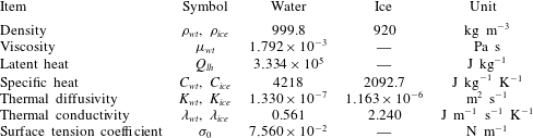
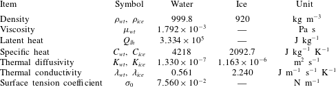
Physical properties of water and ice at 273.15 K.
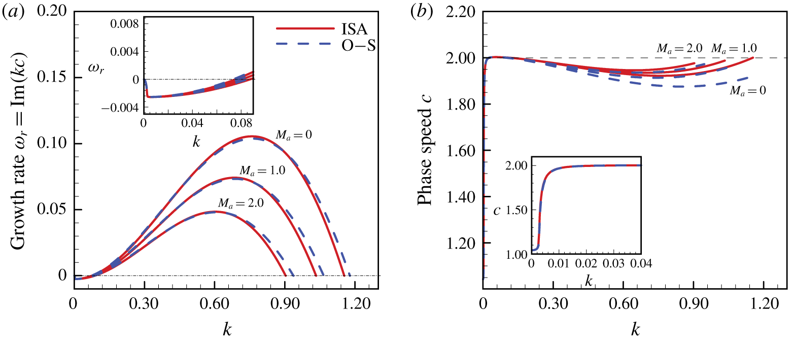
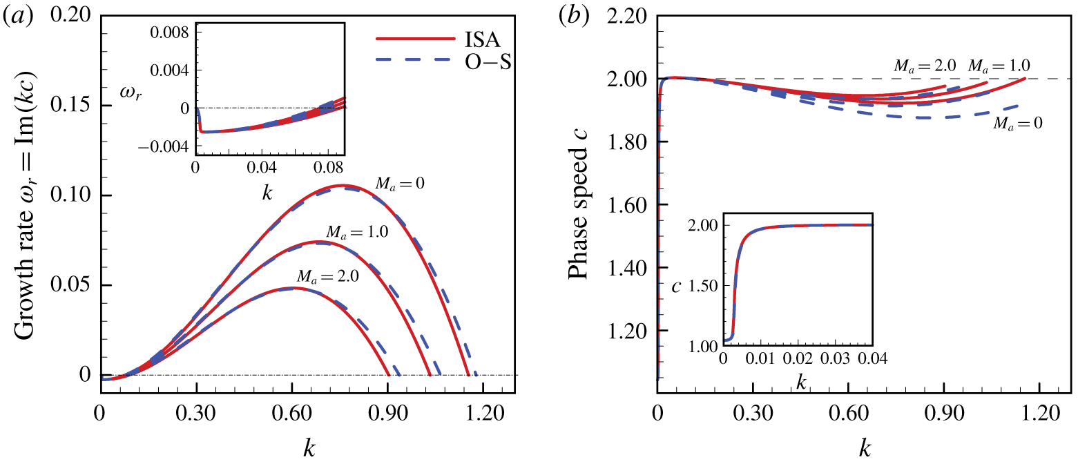
(a) Growth rate  $\text{Im}(kc)$, and (b) phase speed
 $c$ of linear perturbation waves versus wavenumber
 $k$ for different Marangoni number
 $M_{a}$ with
 $T_{air}=0.8$,
 $Re_{\unicode[STIX]{x1D700}}=We_{\unicode[STIX]{x1D700}}=1.0$,
 $Bi=5.0$,
 $St=0.0687$,
 $Pr=13.4733$,
 $\unicode[STIX]{x1D6FC}=8.7460$,
 $\unicode[STIX]{x1D6FD}=3.9929$ and
 $\unicode[STIX]{x1D712}=0.0798$. The solid lines are from the linear instability analysis of the IBL model and the dashed lines are from the Orr–Sommerfeld calculation. The profiles with small wavenumber
 $k$ are zoomed in and shown in the small window. The cut-off wavenumbers
 $k_{cl}$ and
 $k_{cu}$ denote the critical wavenumbers where the growth rate is positive with
 $k\in [k_{cl},k_{cu}]$.
3 Linear instability analysis
It is useful to examine the linear instability of the system obtained in the previous section to test the accuracy of the depth-averaged IBL model and describe its dynamics (Miladinova et al. Reference Miladinova, Slavtchev, Lebon and Legros2002; Samanta, Ruyer-Quil & Goyeau Reference Samanta, Ruyer-Quil and Goyeau2011). The physical properties of water and ice are listed in table 1, which are assumed to be constants independent of temperature. For the typical case studied here, if  $H_{wt}\sim 2\times 10^{-4}~\text{m}$ and
 $\unicode[STIX]{x0394}T\sim 10~\text{K}$ are selected, we have
 $Re\sim 10$,
 $St\sim 10^{-1}$ and
 $We\sim 10^{-2}$. Thus, the condition (2.30) is satisfied. We perturb (2.36)–(2.40) about the Nusselt solution shown in (2.16) with the form of normal modes
 $$\begin{eqnarray}\displaystyle (q,h_{wt},h_{ice},g_{wt},g_{ice}) & = & \displaystyle \left(\frac{2}{3},1,\unicode[STIX]{x1D6FD}\left(1+\frac{1}{Bi}\right)\frac{1-T_{air}}{T_{air}},\frac{Bi}{1+Bi}T_{air},\frac{Bi}{\unicode[STIX]{x1D6FD}(1+Bi)}T_{air}\right)\nonumber\\ \displaystyle & & \displaystyle +\,(Q,H_{wt},H_{ice},G_{wt},G_{ice})\exp [\text{i}k(x-ct)],\end{eqnarray}$$
and linearize for  $(Q,H_{wt},H_{ice},G_{wt},G_{ice})\rightarrow 0$, which is the infinitesimal amplitude of the perturbation with wavenumber
 $k$ and celerity
 $c$. This yields a generalized complex eigenvalue problem (see appendix A). It can be solved numerically by using the software package MATLAB based on the QZ algorithm. In figure 2 we show the growth rate
 $\unicode[STIX]{x1D714}_{r}=\text{Im}(kc)$ and phase speed
 $c$ as a function of the wavenumber
 $k$. For the perturbation with small wavenumber
 $k$, the growth rates and phase speed predicted by the IBL model are relatively close to those obtained by the exact Orr–Sommerfeld equations. This shows a reassuring agreement with particularly good capture of the perturbation growth rates and phase speeds, especially in the case of long-wavelength perturbation. By inspection of figure 2(a), it can be found that the growth rates of perturbation decrease with increasing
 $M_{a}$. The thermocapillary effect acts to stabilize the flow of the water film. This is different from the previous results, where the liquid film is heated from the bottom substrate in the absence of phase transition (Scheid et al. Reference Scheid, Ruyer-Quil, Kalliadasis, Velarde and Zeytounian2005). Moreover, there are two cut-off wavenumbers of
 $k_{cl}$ and
 $k_{cu}$. The growth rate
 $\unicode[STIX]{x1D714}_{r}$ is positive for
 $k\in [k_{cl},k_{cu}]$. Since the surface tension plays a stabilizing role in the infinitesimal perturbation, especially for the perturbation with a short wavelength, it is reasonable that the growth rate
 $\unicode[STIX]{x1D714}_{r}$ is negative for the large wavenumber
 $k>k_{cu}$. Here, an interesting phenomenon is that the growth rate is also negative for the perturbation with a small wavenumber (
 $k<k_{cl}$). It suggests that the phase transition plays a stabilizing role in the flow with long-wavelength perturbations. The corresponding mechanisms are explained in the following section, according to the long-wavelength instability analysis of the system.
3.1 Long-wavelength instability analysis
In this section we study the long-wavelength instability properties of the system in the long-wavelength limit, i.e.  $k\rightarrow 0$. The perturbation quantities can be expanded as
 $$\begin{eqnarray}\displaystyle (Q,H_{wt},H_{ice},G_{wt},G_{ice},c) & = & \displaystyle (Q_{0},H_{wt,0},H_{ice,0},G_{wt,0},G_{ice,0},c_{0})\nonumber\\ \displaystyle & & \displaystyle +\,k(Q_{1},H_{wt,1},H_{ice,1},G_{wt,1},G_{ice,1},c_{1})+O(k^{2}).\end{eqnarray}$$
The corresponding growth rate of the perturbation can be expressed up to  $O(k^{3})$ as
 $$\begin{eqnarray}\unicode[STIX]{x1D714}_{r}=\text{Im}(kc)=k\text{Im}(c_{0}+kc_{1})+O(k^{3}).\end{eqnarray}$$
As shown in Appendix B for the detailed derivation process, we substitute (3.2) into (A 1)–(A 5) and items with the same order of  $k$ are equated separately (Weinstein & Kurz Reference Weinstein and Kurz1991). We focus on the effect of phase transition on the flow instability. The thermocapillary effect is excluded by assuming that
 $M_{a}=0$. In (B 5) we know that
 $c_{0}$ is a real number, which denotes marginal stability. According to (3.3), the system stability is to be determined by the first-order solution
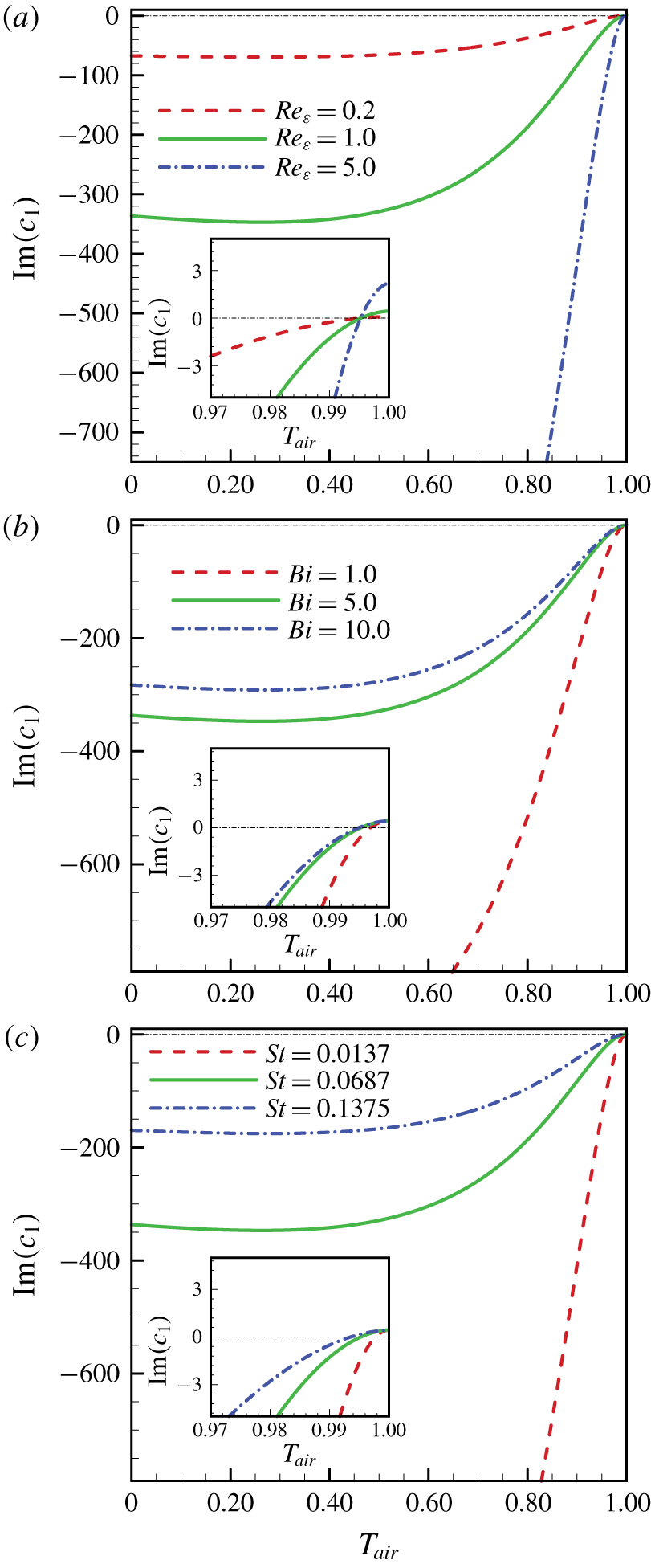
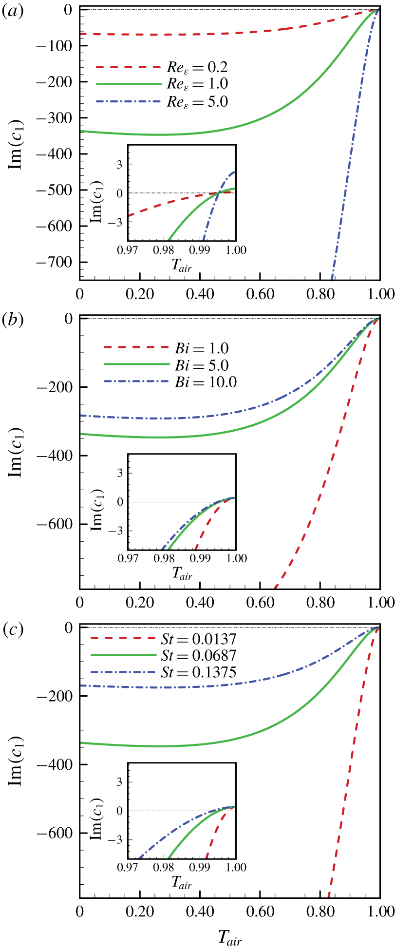
 $c_{1}$, which is expressed analytically in (B 11). In figure 3 we show the effects of flow parameters on the growth rate of long-wavelength perturbation. For small
 $T_{air}$, the value of
 $\text{Im}(c_{1})$ is negative definite. According to (3.3), we know that the flow is linearly stable for long-wavelength perturbations. However, as
 $T_{air}$ approaches 1.0 (
 $0.0<T_{air}<1.0$), the value of
 $\text{Im}(c_{1})$ tends to be positive. The flow is linearly unstable for long-wavelength perturbations. The corresponding wave celerity
 $c_{0}$, which is defined in (B 5), tends to be 2.0. This is consistent with the results presented by Yih (Reference Yih1963) (with a rescaling applied as a different normalization of the steady-state flow solution is taken here). By definition, the wall temperature
 $T_{wall}=T_{air}-1$ approaches zero while
 $T_{air}\rightarrow 1.0$. From (2.17) we know that the thickness of the unperturbed ice sheet tends to be zero. Physically, this may indicate that the phase transition phenomenon (between ice and water) is very weak. The flow instability is mainly induced by the flow inertia. This can also be found from (B 11), where the second and third terms on the right-hand side approach zero as
 $T_{air}\rightarrow 1.0$. The growth rate of perturbation depends on the first term on the right-hand side of (B 11), which represents the effects of the flow inertia. Thus, we can conclude that the phase transition plays a stabilizing role in the long-wavelength perturbation. According to (B 11), the growth rate of the long-wavelength perturbation is proportional to
 $Re_{\unicode[STIX]{x1D700}}$. Thus, the region of
 $T_{air}$ (
 $0.995<T_{air}<1.0$), which corresponds to a positive value of
 $\text{Im}(c_{1})$, is independent of the Reynolds number
 $Re_{\unicode[STIX]{x1D700}}$, as illustrated in figure 3(a). However, as depicted in figures 3(b) and 3(c), these regions expand with increasing Biot
 $Bi$ and Stefan
 $St$ numbers. According to (B 11), as
 $T_{air}\rightarrow 1.0$, we have
 $\text{Im}(c_{1})\rightarrow 4Re_{\unicode[STIX]{x1D700}}/9$, which is independent to
 $Bi$ and
 $St$. Again, this shows the flow instability is dominated by flow inertia when the phase transition is absent.
Growth rate  $\text{Im}(c_{1})$ versus
 $T_{air}$ for various (a) Reynolds number
 $Re_{\unicode[STIX]{x1D700}}$ with
 $Bi=5.0$,
 $St=0.0687$; (b) Biot number
 $Bi$ with
 $Re_{\unicode[STIX]{x1D700}}=1.0$,
 $St=0.0687$; (c) Stefan number
 $St$ with
 $Re_{\unicode[STIX]{x1D700}}=1.0$,
 $Bi=5.0$. The results are obtained from the long-wavelength approximation without including the thermocapillary effect (
 $M_{a}=0.0$). The rest parameters are
 $We_{\unicode[STIX]{x1D700}}=1.0$,
 $Pr=13.4733$,
 $\unicode[STIX]{x1D6FC}=8.7460$,
 $\unicode[STIX]{x1D6FD}=3.9929$ and
 $\unicode[STIX]{x1D712}=0.0798$. The profiles with
 $T_{air}$ around 1.0 are zoomed in and shown in the small window.
3.2 Effect of phase transition on the flow instability
Since the IBL model has been shown to capture the linear instability properties of the film adequately, we can now make use of (2.36)–(2.40) to gain insight into the influence of phase transition on the system linear instability. According to the corresponding linearized equations (A 1) and (A 2), we have
 $$\begin{eqnarray}cH_{wt}=Q-\frac{\text{i}(1.0-\unicode[STIX]{x1D712})}{Pr}\frac{St}{kRe_{\unicode[STIX]{x1D700}}}(\unicode[STIX]{x1D6FD}G_{ice}-G_{wt}).\end{eqnarray}$$
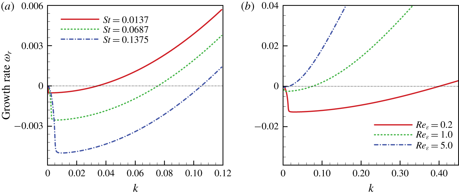
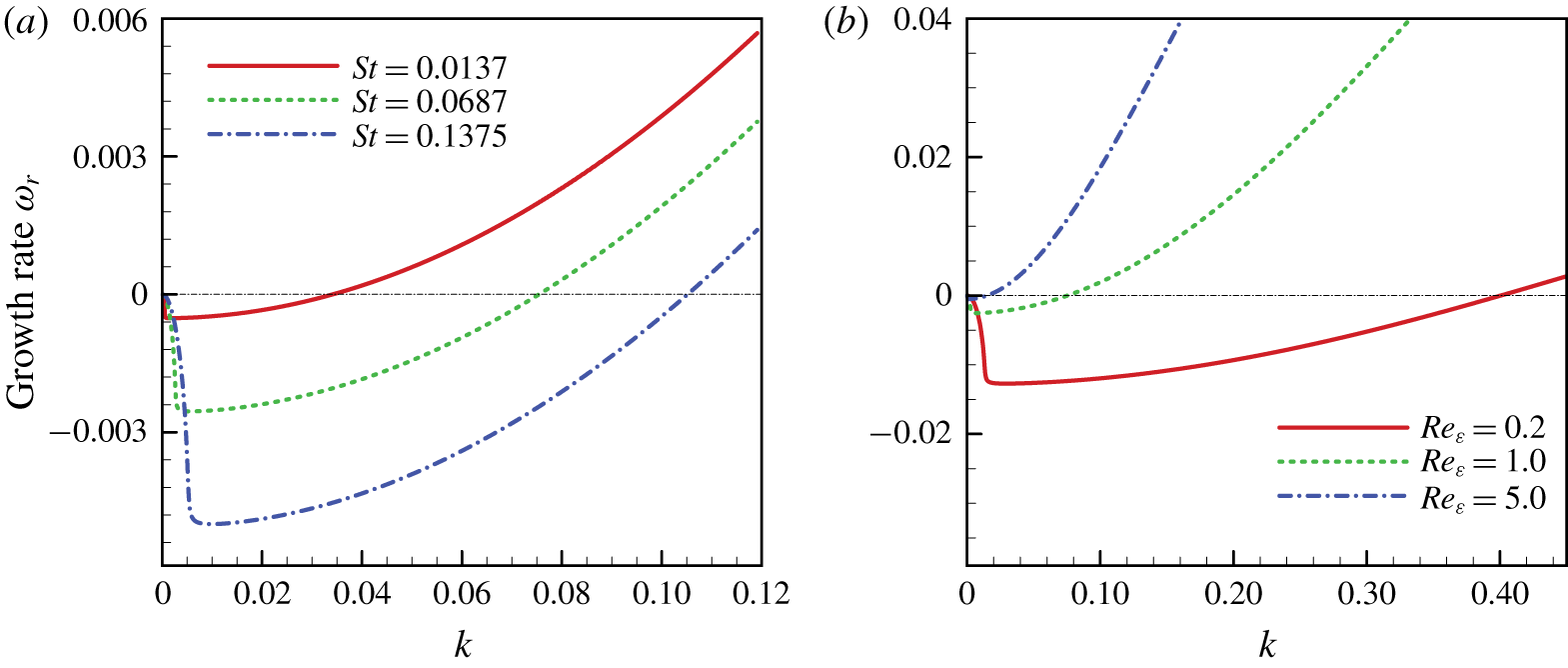
From comparisons with previous literature (Prokopiou, Cheng & Chang Reference Prokopiou, Cheng and Chang1991), we know that the second term on the right-hand side of (3.4) indicates the effect of phase transition on the system linear instability. The perturbation of flow rate can be adjusted due to the presence of phase transition, which is proportional to the Stefan number  $St$ but inversely proportional to the wavenumber
 $k$ and the flow Reynolds number
 $Re_{\unicode[STIX]{x1D700}}$. The intermediate band of wavenumbers, which is linear stable due to the influence of phase transition, expands with increasing
 $St$ (or decreasing
 $Re_{\unicode[STIX]{x1D700}}$), as illustrated in figure 4. Moreover, in figure 4(a) the value of
 $\text{d}\unicode[STIX]{x1D714}_{r}/\text{d}k$ at
 $k\rightarrow 0$ increases with increasing
 $St$ (the absolute value of
 $\text{d}\unicode[STIX]{x1D714}_{r}/\text{d}k$ reduces since
 $\text{d}\unicode[STIX]{x1D714}_{r}/\text{d}k<0.0$). This is consistent with those presented in figure 3(c), where
 $\text{d}\unicode[STIX]{x1D714}_{r}/\text{d}k$ is proportional to
 $\text{Im}(c_{1})$, as expressed in (3.3). In figure 4(b),
 $\text{d}\unicode[STIX]{x1D714}_{r}/\text{d}k$ at
 $k\rightarrow 0$ decreases with increasing
 $Re_{\unicode[STIX]{x1D700}}$. Similar results can also be drawn from figure 3(a).
Effect of (a)  $St$ with
 $Re_{\unicode[STIX]{x1D700}}=1.0$ and (b)
 $Re_{\unicode[STIX]{x1D700}}$ with
 $St=0.0687$ on the growth rate of linear perturbation waves for
 $T_{air}=0.8$,
 $We_{\unicode[STIX]{x1D700}}=1.0$,
 $Bi=5.0$,
 $M_{a}=0$,
 $Pr=13.4733$,
 $\unicode[STIX]{x1D6FC}=8.7460$,
 $\unicode[STIX]{x1D6FD}=3.9929$ and
 $\unicode[STIX]{x1D712}=0.0798$. Here, in order to manifest the stabilization effect of phase transition on long-wavelength perturbation, the growth rates of small wavenumber perturbations are only presented.
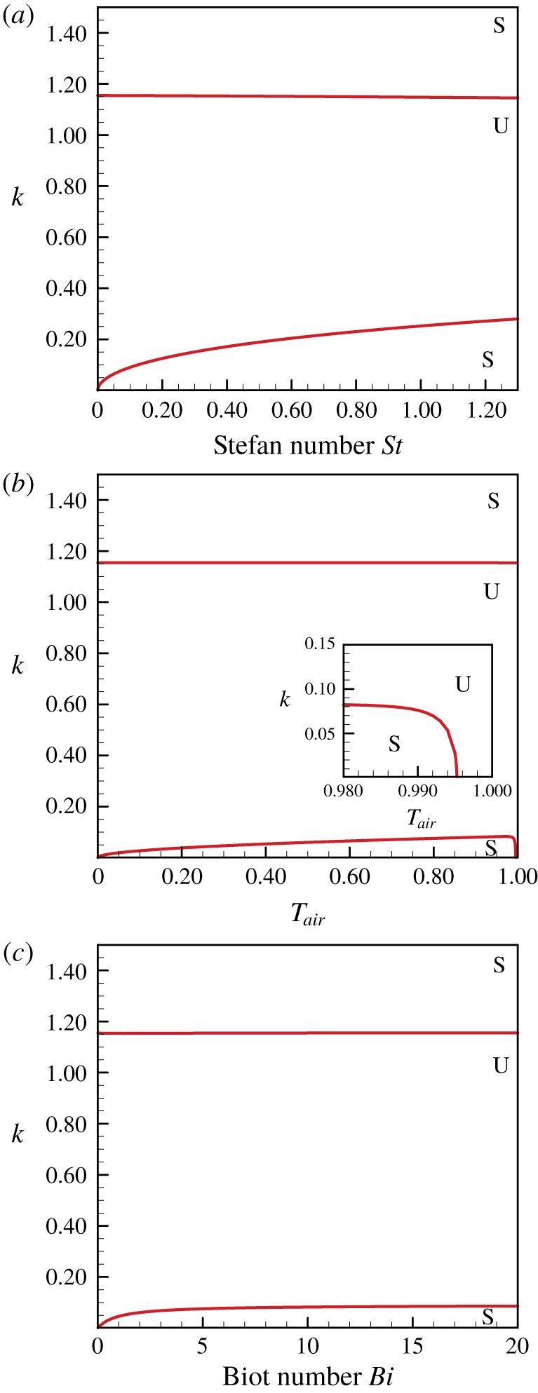
Neutral stability curves on the (a)  $St{-}k$ plane with
 $T_{air}=0.8$ and
 $Bi=5.0$; (b)
 $T_{air}{-}k$ with
 $St=0.0687$ and
 $Bi=5.0$; (c)
 $Bi{-}k$ plane with
 $T_{air}=0.8$ and
 $St=0.0687$. The thermocapillary effect is excluded by setting
 $M_{a}=0.0$ with
 $Re_{\unicode[STIX]{x1D700}}=We_{\unicode[STIX]{x1D700}}=1.0$. The rest parameters are
 $Pr=13.4733$,
 $\unicode[STIX]{x1D6FC}=8.7460$,
 $\unicode[STIX]{x1D6FD}=3.9929$ and
 $\unicode[STIX]{x1D712}=0.0798$. Symbol ‘S’ stands for the linear stable zone while ‘U’ stands for the linear unstable zone.
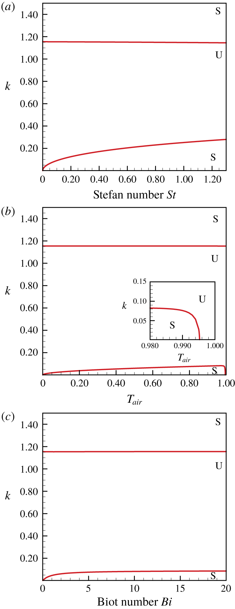
In figure 5 we show the neutral stability curves, which delineate the boundary between the stable and unstable regions. In figure 5(a) there are two branches which separate the  $St{-}k$ plane into three parts. For the flow with small wavenumber perturbation (
 $k<k_{cl}$), the linearly stable zone, which is located below the lower branch of the neutral curve, expands with increasing
 $St$. Again, this suggests that the phase transition acts to stabilize the flow with long-wavelength perturbations. However, for the perturbation with a large wavenumber, the linearly stable zone, which is located above the upper branch of the neutral curve, seems not to change. This is attributed to the fact that the short-wavelength perturbations are suppressed dominantly by the surface tension unrelated to the phase transition. In figure 5(b) we show the neutral stability curves on the
 $T_{air}{-}k$ plane. For
 $0<T_{air}<0.995$, a linearly stable zone for the perturbations with a small wavenumber (
 $k<k_{cl}$) can be observed. As mentioned previously, this is attributed to the influences of the phase transition at the ice–water interface. As
 $T_{air}\rightarrow 0$, in our model, it indicates that the air temperature above the water film approaches the freezing point. From (3.1), the temperature gradients
 $g_{wt}$ and
 $g_{ice}$ tend to be zero. Thus, according to (2.40), we know that the phase transition is too weak to stabilize the long-wavelength perturbation. When
 $T_{air}$ approaches 0.995, as shown in the zoomed window in figure 5(b), the flow tends to be linear unstable even for the long-wavelength perturbations, i.e.
 $k_{cl}\rightarrow 0$. This is consistent with the result of the long-wavelength instability analysis, as shown in figure 3(a). For the perturbations with a large wavenumber, the flow is stabilized linearly by surface tension, and the linearly stable zone does not change with
 $T_{air}$. This is entirely similar to those profiled in figure 5(a). The neutral stability curves on the
 $Bi{-}k$ plane are shown in figure 5(c). In this study, as presented in (2.10) or (2.29), Newton’s law of cooling is adopted at the free surface. As
 $Bi\rightarrow 0$, where the interface is entirely insulated from the air, the temperature of the water film would tend to be near the freezing point. Similar to those with
 $T_{air}\rightarrow 0$, the phase transition is very weak. The linearly stable zone (
 $k<k_{cl}$) caused by the phase transition tends to shrink. On the other hand, as
 $Bi$ increases to a substantial value, the temperature of the air–water free surface approaches that of the surrounding air. The effect of
 $Bi$ tends to be saturated, and the stable zone does not increase anymore.
3.3 Effect of thermocapillary on the flow instability
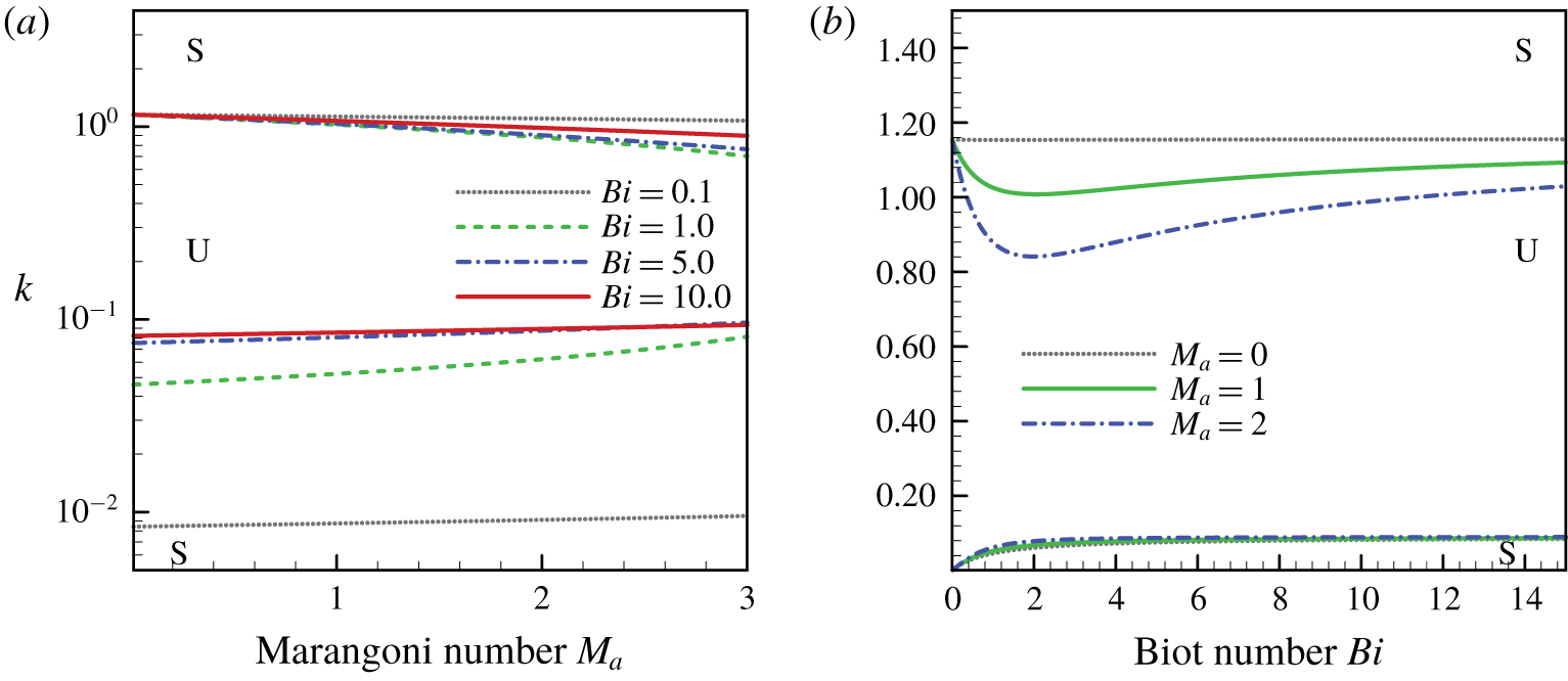
Neutral stability curves (a) on the  $M_{a}{-}k$ plane with various
 $Bi$, and (b) on the
 $Bi{-}k$ plane with various
 $M_{a}$, for
 $Re_{\unicode[STIX]{x1D700}}=1.0$,
 $We_{\unicode[STIX]{x1D700}}=1.0$,
 $T_{air}=0.8$,
 $St=0.0687$. The values of the rest parameters are
 $Pr=13.4733$,
 $\unicode[STIX]{x1D6FC}=8.7460$,
 $\unicode[STIX]{x1D6FD}=3.9929$ and
 $\unicode[STIX]{x1D712}=0.0798$. Symbol ‘S’ stands for the linear stable zone while ‘U’ stands for the linear unstable zone.

We now examine the effect of thermocapillary on the linear instability properties of the system. It is well known that the thermocapillary stress on the free surface caused by the surface gradient of temperature has a distinct effect on the hydrodynamics of the liquid film (Kalliadasis et al. Reference Kalliadasis, Kiyashko and Demekhin2003b; Ruyer-Quil et al. Reference Ruyer-Quil, Scheid, Kalliadasis, Velarde and Zeytounian2005; Scheid et al. Reference Scheid, Ruyer-Quil, Kalliadasis, Velarde and Zeytounian2005). In figure 6(a) we show the neutral stability curve on the  $M_{a}{-}k$ plane, with the Biot number
 $Bi$ being a parameter. As the Marangoni number
 $M_{a}$ increases, the thermocapillary effect is intensified, and the unstable zone tends to become smaller. Similar results can also be drawn in figure 2, where the band of the unstable wavenumber
 $k$ narrows with increasing
 $M_{a}$ (amplifying
 $k_{cl}$ while narrowing
 $k_{cu}$). It denotes that the thermocapillary effect plays a stabilizing role in the linear instability of the system. This effect becomes weak when
 $Bi$ is extremely small (e.g.,
 $Bi=0.1$). This is attributed to the fact that, for small
 $Bi$, the temperature distribution of the water film tends toward uniformity around the freezing point. The corresponding thermocapillary stress becomes weak. In figure 6(b) we show the neutral stability curve on the
 $Bi{-}k$ plane with the Marangoni number
 $M_{a}$ being a parameter. As
 $Bi$ increases, the unstable zone is gradually reduced and then gradually increased. This indicates that the thermocapillary effect is intensified firstly with increasing
 $Bi$. However, as
 $Bi$ increases to a substantial value, similar to those presented in figure 5(c), the effect of
 $Bi$ tends to be saturated. The temperature on the air–water free surface tends to be uniform and approaches the temperature of the surrounding air
 $T_{air}$. As a result, the thermocapillary effect is weakened.
4 Temporal stability analysis
4.1 Evolution of primary long-wavelength perturbation
From the previous section, it appears that the initial perturbation with a short wavelength ( $k>k_{cu}$) will decay under the linear instability framework owing to the stabilizing role of surface tension. This can be extended to the nonlinear situation (Ramaswamy, Chippada & Joo Reference Ramaswamy, Chippada and Joo1996). According to the linear instability analysis, the long-wavelength perturbation with wavenumber
 $k<k_{cl}$ can also be stabilized due to the presence of phase transition. In this section we focus on the nonlinear evolution of the initial long-wavelength perturbation. The results of the nonlinear evolution of the system are presented in terms of the film thickness
 $h_{wt}(x,t)$ at various instants of time,
 $$\begin{eqnarray}h_{wt}(x,t)=\mathop{\sum }_{n=-N}^{N}A_{n}(t)\exp (\text{i}nkx),\end{eqnarray}$$
where  $2N$ is the number of mesh divisions in the streamwise direction. This is equal to the round-off number of
 $256/k$. Here
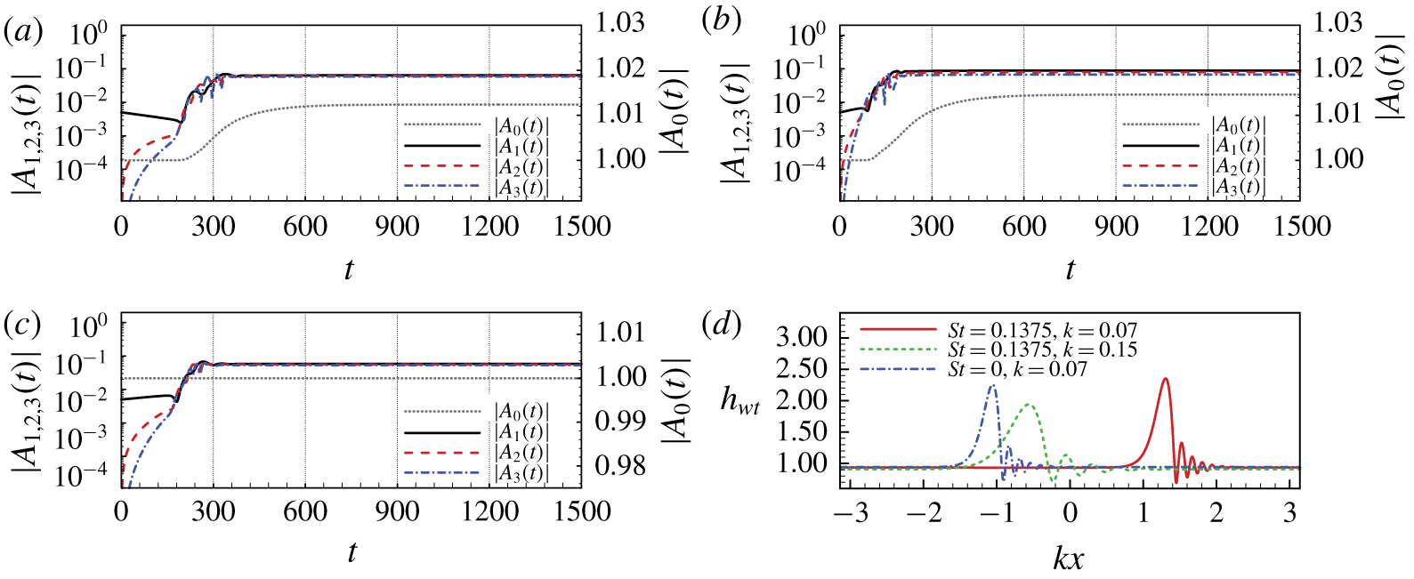
 $A_{n}(t)$ is the spatial-spectral coefficient, which can be used to quantify the system dynamics of the nonlinear process. As presented in (3.1), the thickness of the tranquil water film is 1.0. The fundamental perturbation mode is assumed to be a sine wave with amplitude equaling 0.01. The dynamic of the nonlinear process can be quantified through
 $A_{n}(t)$. According to figures 4 and 5(a), for the long-wavelength perturbation mode
 $k=0.07$, the wavenumber is smaller than the cut-off wavenumber
 $k_{cl}=0.105$ (with
 $T_{air}=0.8$,
 $Re_{\unicode[STIX]{x1D700}}=We_{\unicode[STIX]{x1D700}}=1.0$,
 $St=0.1375$,
 $Bi=5.0$ and
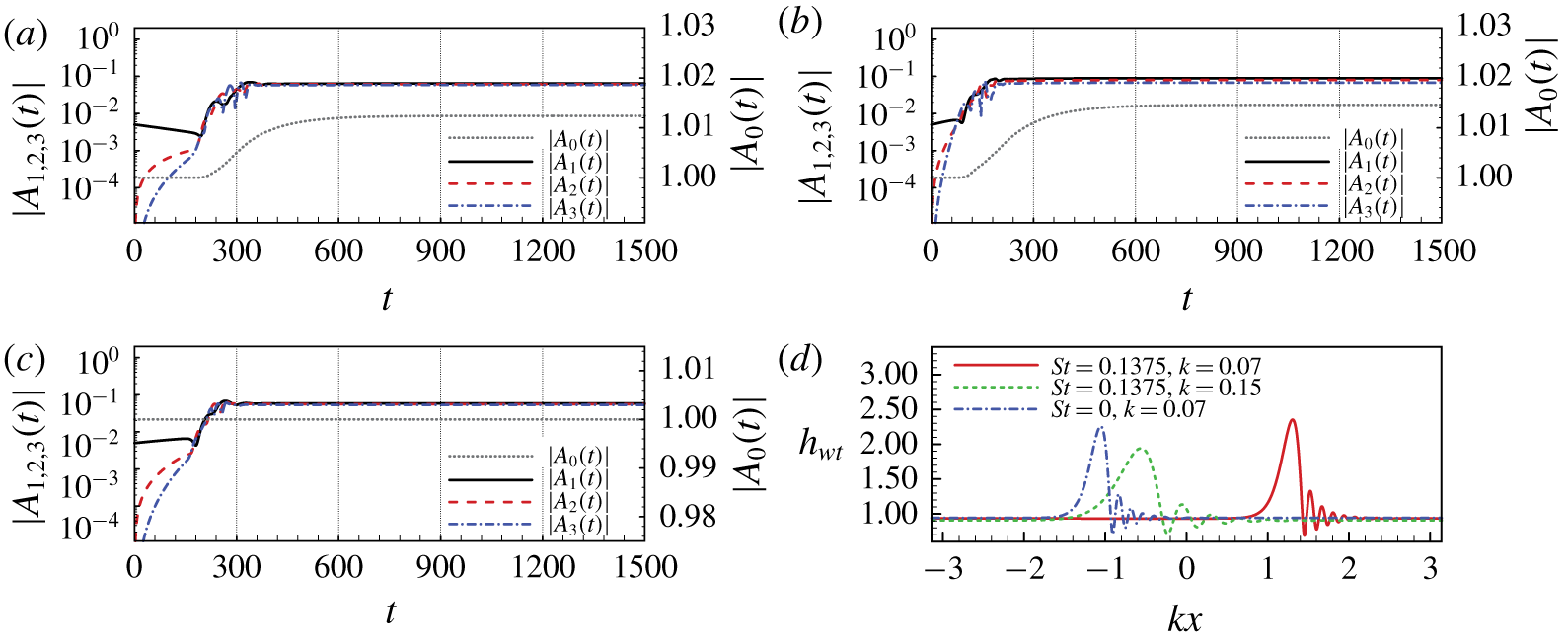
 $M_{a}=0.0$). Based on the linear instability analysis, the phase transition acts to stabilize it. As illustrated in figure 7(a), the fundamental mode (
 $k=0.07$ and quantified with
 $A_{1}(t)$) decays initially. However, due to the presence of nonlinearity, the corresponding high-order harmonics, which can be quantified with
 $A_{2}(t),A_{3}(t),\ldots \,$, are excited and grow rapidly. When the intensities of the harmonics become almost as strong as the fundamental mode, attributed to the nonlinear interaction between the fundamental and the harmonic modes, the fundamental mode tends to grow. This is different from the evolution of the short-wavelength perturbation (
 $k>k_{cu}$), where the harmonic modes also decay due to the stabilizing role of the surface tension (Ramaswamy et al. Reference Ramaswamy, Chippada and Joo1996). In figure 7(b) the wavenumber of the fundamental mode is
 $k=0.15$, which is larger than the cut-off wavenumber
 $k_{cl}=0.105$. It shows that the fundamental mode grows exponentially initially, and the first several harmonics grow rapidly as well. Similar trends can also be discovered in figure 7(c), where the phase transition is excluded by setting
 $St=0.0$. The wavenumber of the fundamental mode is also set to
 $k=0.07$. In figures 7(a) and 7(b), the spatial-spectral coefficient
 $A_{0}$, which indicates the average thickness of the water film, gradually increases and approaches to 1.012 and 1.015, respectively. However, in figure 7(c), since there is no phase transition (
 $St=0.0$), the average thickness of the water film is constant. Due to the conservation of mass,
 $A_{0}$ equals 1.0 permanently. Comparing figures 7(a) and 7(c) show that the phase transition does act to suppress the growth of the fundamental long-wavelength mode during the initial evolution stage. After that, due to the interaction between the fundamental and the harmonic modes, they all tend to grow. However, the growth will be arrested owing to the stabilizing role of surface tension (Ramaswamy et al. Reference Ramaswamy, Chippada and Joo1996), eventually resulting in the solitary-like steady travelling waves (Shkadov & Sisoev Reference Shkadov and Sisoev2004; Samanta et al. Reference Samanta, Ruyer-Quil and Goyeau2011), as illustrated in figure 7(d), where the profiles of the water film are presented at time
 $t=1470$.
Evolution of the spatial-spectral coefficient  $|A_{n}(t)|$ for initial perturbation wavenumber (a)
 $k=0.07$,
 $St=0.1375$; (b)
 $k=0.15$,
 $St=0.1375$; (c)
 $k=0.07$,
 $St=0.0$ and (d) the solitary-like steady travelling waves correspond to the different initial perturbation modes at time
 $t=1470$. The values of the rest parameters are
 $Re_{\unicode[STIX]{x1D700}}=We_{\unicode[STIX]{x1D700}}=1.0$,
 $Bi=5.0$,
 $T_{air}=0.8$,
 $M_{a}=0.0$,
 $Pr=13.4733$,
 $\unicode[STIX]{x1D6FC}=8.7460$,
 $\unicode[STIX]{x1D6FD}=3.9929$ and
 $\unicode[STIX]{x1D712}=0.0798$.
4.2 Steady travelling waves
Let us now consider the stationary solutions of the system in the form of  $q(\unicode[STIX]{x1D709})$,
 $h_{wt}(\unicode[STIX]{x1D709})$,
 $h_{ice}(\unicode[STIX]{x1D709})$,
 $g_{wt}(\unicode[STIX]{x1D709})$ and
 $g_{ice}(\unicode[STIX]{x1D709})$. Here,
 $\unicode[STIX]{x1D709}=k(x-ct)$, where
 $k$ is the wavenumber and
 $c$ is the celerity of the travelling waves. We have
 $$\begin{eqnarray}\frac{\unicode[STIX]{x2202}}{\unicode[STIX]{x2202}t}=-ck\frac{\unicode[STIX]{x2202}}{\unicode[STIX]{x2202}\unicode[STIX]{x1D709}},\quad \frac{\unicode[STIX]{x2202}}{\unicode[STIX]{x2202}x}=k\frac{\unicode[STIX]{x2202}}{\unicode[STIX]{x2202}\unicode[STIX]{x1D709}}.\end{eqnarray}$$
Similar to those works in previous literature (Trifonov & Tsvelodub Reference Trifonov and Tsvelodub1991; Chang, Demekhin & Kopelevich Reference Chang, Demekhin and Kopelevich1993; Sisoev et al. Reference Sisoev, Matar, Craster and Kumar2010; Zhou et al. Reference Zhou, Peng, Zhang and Zhuge2016), after substituting (4.2) into (2.36)–(2.40), the system for steady travelling waves can be derived. As shown in appendix C, it can be completed with supplementing an integral condition (C 6) and a phase condition (C 7). Equation (C 6) is also a mass conservation condition. It ensures that the wave carries the same mass (including the mass of the ice sheet) as the smooth Nusselt flow of the same periodicity. In this study, the pseudo-spectral method is used for the spatial discretization of (C 1)–(C 7). The Newton–Kantorovich approach is adopted to obtain the travelling wave solutions numerically. The bifurcation profiles are obtained by using the continuation method (Zhou et al. Reference Zhou, Peng, Zhang and Zhuge2016), which starts from the neutral point of linear instability with  $k=k_{cu}$. It is worth noting that, for a single wavenumber
 $k$, there exist multiple solutions. The bifurcation structures of the solutions are very complex (Shkadov & Sisoev Reference Shkadov and Sisoev2004; Sisoev et al. Reference Sisoev, Matar, Craster and Kumar2010). Here, two leading families of waves, named
 $\unicode[STIX]{x1D6FE}^{-1}$ and
 $\unicode[STIX]{x1D6FE}^{1}$ waves, are only considered. The
 $\unicode[STIX]{x1D6FE}^{-1}$ waves travel at a slower speed than the linear marginal waves with a shape made of one or several troughs followed by capillary ripples. These waves are the ones branching off the Nusselt solution at the cut-off wavenumber
 $k_{cu}$ corresponding to the Hopf bifurcation point. The
 $\unicode[STIX]{x1D6FE}^{1}$ waves are fast waves made of one or several humps preceded by front-running capillary ripples, which bifurcates from the
 $\unicode[STIX]{x1D6FE}^{-1}$ family by flipping or period-doubling (Chang & Demekhin Reference Chang and Demekhin2002). Generally, the bifurcation diagram is similar to those presented by Shkadov & Sisoev (Reference Shkadov and Sisoev2004). However, the presence of the phase transition and thermocapillary effect tends to induce some differences.
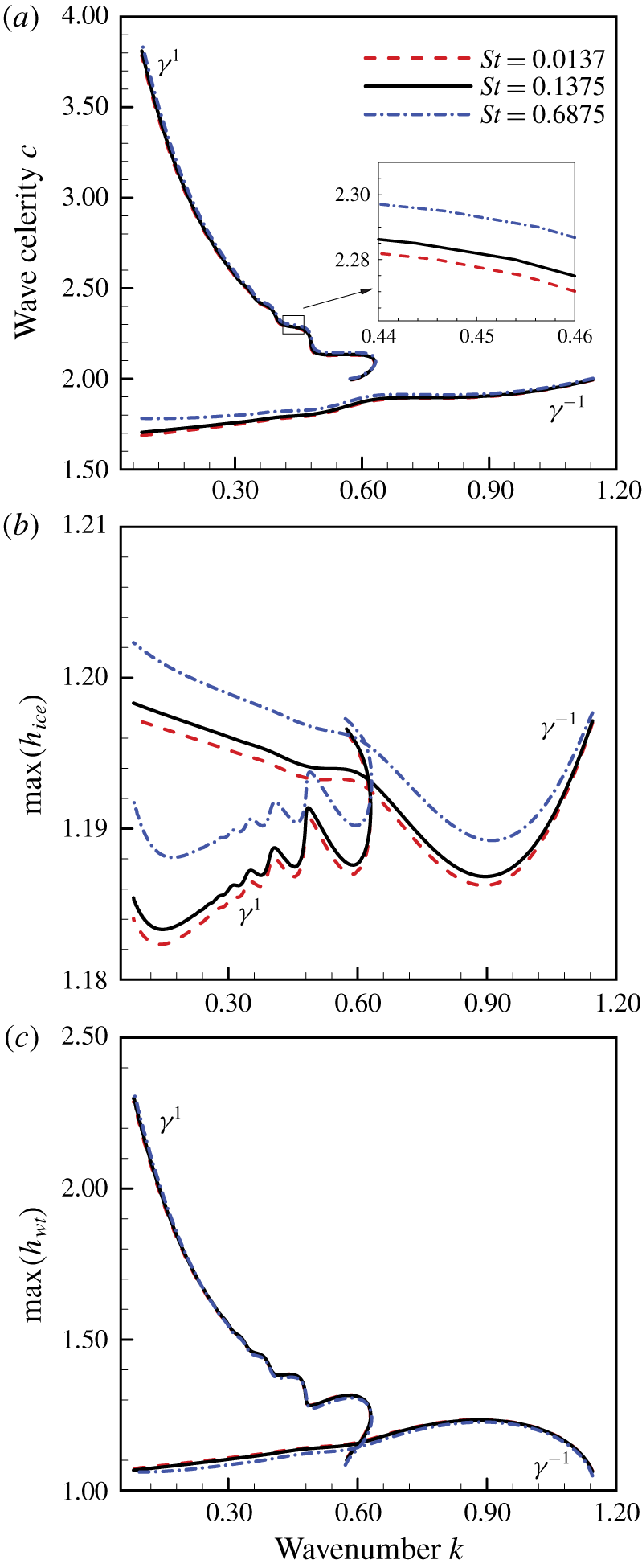
(a) Wave celerity  $c$, (b) maximum thickness of the ice sheet
 $\max (h_{ice})$ and (c) maximum thickness of the water film
 $\max (h_{wt})$ of
 $\unicode[STIX]{x1D6FE}^{-1}$ and
 $\unicode[STIX]{x1D6FE}^{1}$ travelling waves as functions of the wavenumber
 $k$ for various Stefan numbers
 $St$ with
 $Re_{\unicode[STIX]{x1D700}}=We_{\unicode[STIX]{x1D700}}=1.0$,
 $Bi=5.0$,
 $T_{air}=0.8$ and
 $M_{a}=0.0$. The values of the rest parameters are
 $Pr=13.4733$,
 $\unicode[STIX]{x1D6FC}=8.7460$,
 $\unicode[STIX]{x1D6FD}=3.9929$ and
 $\unicode[STIX]{x1D712}=0.0798$.

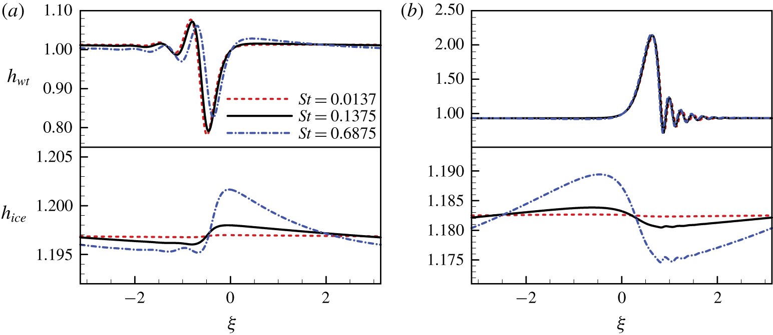
Wave profiles for various  $St$, while
 $k=0.11$: (a)
 $\unicode[STIX]{x1D6FE}^{-1}$ wave; (b)
 $\unicode[STIX]{x1D6FE}^{1}$ wave. See the caption of figure 8 for other parameters.

Figure 8 depicts the characteristics of  $\unicode[STIX]{x1D6FE}^{-1}$ and
 $\unicode[STIX]{x1D6FE}^{1}$ with various Stefan numbers
 $St$. The wave celerity increases slightly with increasing Stefan number
 $St$. It is more evident for the
 $\unicode[STIX]{x1D6FE}^{-1}$ waves with a small wavenumber
 $k$, as illustrated in figure 8(a). This may suggest that the phase transition acts to weaken the dispersion property within the system. From (2.17) we know that the thickness of the unperturbed ice sheet is independent of
 $St$. However, according to (C 2), the variation of the ice–water interface position caused by phase change will be enhanced as
 $St$ increases. This can also be seen in figure 8(b), where the maximum thickness of the ice sheet dilates with increasing
 $St$. In figure 8(c) we show that the maximum thickness of the water film for
 $\unicode[STIX]{x1D6FE}^{-1}$ waves decreases with increasing Stefan number
 $St$, whereas the maximum thickness of the water film for
 $\unicode[STIX]{x1D6FE}^{1}$ waves shows almost no changes. This can also be found in figure 9, where the shapes of the
 $\unicode[STIX]{x1D6FE}^{-1}$ and
 $\unicode[STIX]{x1D6FE}^{1}$ waves are profiled, respectively. For the
 $\unicode[STIX]{x1D6FE}^{1}$ wave, the displacement of the air–water free surface seems to have little change with various
 $St$. However, due to the enhancement of phase transition, the displacement of the ice–water interface increases as
 $St$ becomes larger.
In this study the temperatures of the ambient air and the cold solid wall are taken as constants (e.g.  $T_{air}=0.8$ and
 $T_{wall}=-0.2$). The value of the temperature gradient on both sides of the ice–water interface, i.e.
 $g_{wt}$ and
 $g_{ice}$, are inversely proportional to the thickness of the water film and ice sheet, approximately. In figure 9 the displacement of the air–water free surface is much larger than that of the ice–water interface. Compared with the variation of
 $g_{wt}$, the change of
 $g_{ice}$ can be ignored. According to (C 2), for each given
 $c$ and
 $k$,
 $\unicode[STIX]{x2202}h_{ice}/\unicode[STIX]{x2202}\unicode[STIX]{x1D709}$ is proportional to the difference between
 $g_{wt}$ and
 $g_{ice}$. When the thickness of the water film
 $h_{wt}$ increases,
 $g_{wt}$ tends to decrease. As a result,
 $\unicode[STIX]{x2202}h_{ice}/\unicode[STIX]{x2202}\unicode[STIX]{x1D709}$ drops and could even become negative if the thickness of the water film
 $h_{wt}$ increases continuously. In figure 9(a), corresponding to the trough of the
 $\unicode[STIX]{x1D6FE}^{-1}$ wave at the air–water free surface, a small crest is observed at the ice–water interface. The thickness of the ice sheet
 $h_{ice}$ tends to increase (corresponds to
 $\unicode[STIX]{x2202}h_{ice}/\unicode[STIX]{x2202}\unicode[STIX]{x1D709}>0$), while the thickness of the water film
 $h_{wt}$ decreases. When
 $h_{wt}$ reaches its minimum,
 $\unicode[STIX]{x2202}h_{ice}/\unicode[STIX]{x2202}\unicode[STIX]{x1D709}$ achieves a maximum. After that,
 $\unicode[STIX]{x2202}h_{ice}/\unicode[STIX]{x2202}\unicode[STIX]{x1D709}$ tends to decrease as
 $h_{wt}$ increases. As a result,
 $h_{ice}$ keeps increasing until
 $\unicode[STIX]{x2202}h_{ice}/\unicode[STIX]{x2202}\unicode[STIX]{x1D709}$ becomes negative. Intuitively, the crest of the ice–water interface is located below the front of the trough on the air–water free surface. Similar results can also be found in the
 $\unicode[STIX]{x1D6FE}^{1}$ waves, as illustrated in figure 9(b). The trough of the ice–water interface is formed below the front of the hump on the air–water free surface. The corresponding crest of the ice–water interface is located below the rear of the hump on the air–water free surface.
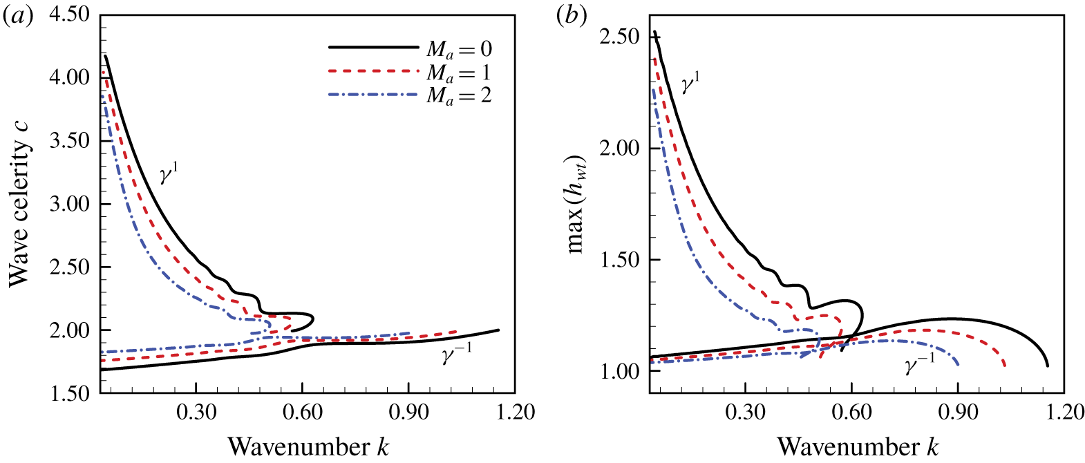
(a) Wave celerity  $c$, (b) maximum thickness of the water film
 $\max (h_{wt})$ of
 $\unicode[STIX]{x1D6FE}^{-1}$ and
 $\unicode[STIX]{x1D6FE}^{1}$ travelling waves as functions of the wavenumber
 $k$ for various Marangoni numbers with
 $Re_{\unicode[STIX]{x1D700}}=We_{\unicode[STIX]{x1D700}}=1.0$,
 $Bi=5.0$,
 $St=0.0687$ and
 $T_{air}=0.8$. The values of the rest parameters are
 $Pr=13.4733$,
 $\unicode[STIX]{x1D6FC}=8.7460$,
 $\unicode[STIX]{x1D6FD}=3.9929$ and
 $\unicode[STIX]{x1D712}=0.0798$.

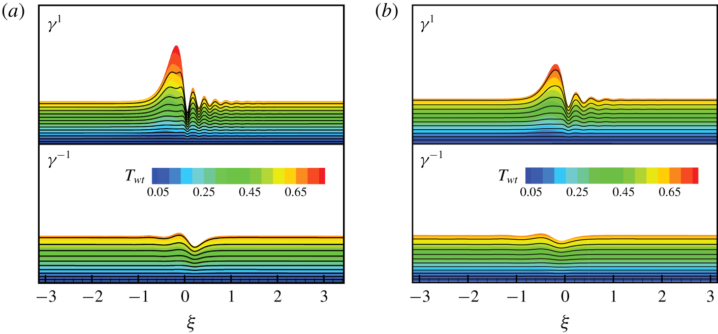
Temperature distribution and streamlines for (a)  $M_{a}=0.0$ and (b)
 $M_{a}=2.0$ at
 $k=0.11$. See the caption of figure 10 for other parameters.

In figure 10 we show the effect of the Marangoni number  $M_{a}$ on the characteristics of the
 $\unicode[STIX]{x1D6FE}^{-1}$ and
 $\unicode[STIX]{x1D6FE}^{1}$ waves. As
 $M_{a}$ increases, the celerity of the
 $\unicode[STIX]{x1D6FE}^{1}$ wave is degraded while the celerity of the
 $\unicode[STIX]{x1D6FE}^{-1}$ wave is promoted. It can be concluded that the thermocapillary effect plays a role in suppressing the dispersion characteristics within the system. Moreover, as
 $M_{a}$ increases, the maximum thickness of the water film for both
 $\unicode[STIX]{x1D6FE}^{1}$ and
 $\unicode[STIX]{x1D6FE}^{-1}$ waves decreases. This may be attributed to the fact that the surface tension at the air–water free surface, defined in (2.8), decreases with increasing temperature. The corresponding thermocapillary traction force at the air–water free surface directs from the crest to the trough of the surface wave. As a result, the height of the wave peak is suppressed and decreases with increasing
 $M_{a}$. In figure 11 we show the wave profiles, temperature distribution and streamlines for different Marangoni numbers
 $M_{a}$. For
 $M_{a}=2.0$, in the presence of the thermocapillary effect, amplitudes of the main humps for both
 $\unicode[STIX]{x1D6FE}^{-1}$ and
 $\unicode[STIX]{x1D6FE}^{1}$ waves are reduced. The corresponding capillary ripples are also suppressed. It is worth noting that the streamlines in figure 11 are plotted in the coordinate system of the travelling wave, which is different from those obtained in the absolute coordinate system in the following § 5.
(a) Wave celerity  $c$, (b) maximum thickness of the water film
 $\max (h_{wt})$ of
 $\unicode[STIX]{x1D6FE}^{-1}$ and
 $\unicode[STIX]{x1D6FE}^{1}$ travelling waves as functions of the wavenumber
 $k$ for various Biot numbers
 $Bi$, while
 $Re_{\unicode[STIX]{x1D700}}=We_{\unicode[STIX]{x1D700}}=1.0$,
 $St=0.0687$,
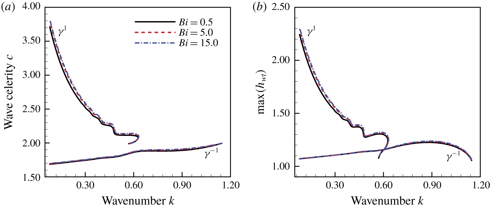
 $T_{air}=0.8$ and
 $M_{a}=0.0$. The values of the rest parameters are similar to those in figure 10.

(a) Wave celerity  $c$, (b) maximum thickness of the water film
 $\max (h_{wt})$ of
 $\unicode[STIX]{x1D6FE}^{1}$ and
 $\unicode[STIX]{x1D6FE}^{-1}$ travelling waves as functions of the wavenumber
 $k$ for various Biot numbers
 $Bi$, while
 $Re_{\unicode[STIX]{x1D700}}=We_{\unicode[STIX]{x1D700}}=1.0$,
 $St=0.0687$,
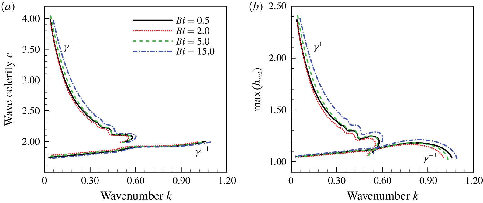
 $T_{air}=0.8$ and
 $M_{a}=1.0$. The values of the rest parameters are similar to those in figure 10.

Figures 12 and 13 depict the effects of the Biot number  $Bi$ on the characteristics of the
 $\unicode[STIX]{x1D6FE}^{1}$ and
 $\unicode[STIX]{x1D6FE}^{-1}$ waves with (
 $M_{a}=1.0$) and without (
 $M_{a}=0.0$) considering the action of thermocapillary effects. According to the definition of
 $Bi$, we know that the heat transport rate from the liquid water to the ambient air is proportional to the value of
 $Bi$. It is understandable that the wave profiles on the air–water free surface do not change much with varying Biot number
 $Bi$. As illustrated in figure 12, for
 $M_{a}=0.0$, which indicates the absence of thermocapillary effects, both the wave celerity and maximum thickness of the water film tend to increase slightly with increasing
 $Bi$. However, as illustrated in figure 13, when the thermocapillary effect is included (
 $M_{a}=1.0$), the bifurcation profiles change obviously with increasing
 $Bi$. For small
 $Bi$, e.g.
 $Bi=0.5$ and 2.0, the celerity of the
 $\unicode[STIX]{x1D6FE}^{1}$ wave is postponed, and the celerity of the
 $\unicode[STIX]{x1D6FE}^{-1}$ wave is promoted slightly with increasing
 $Bi$. This indicates that the role of the thermocapillary effect is intensified with increasing
 $Bi$. However, as
 $Bi$ increases further, e.g.
 $Bi=5.0$ and 15.0, the situation changes completely. The celerity of the
 $\unicode[STIX]{x1D6FE}^{1}$ wave is promoted, while the celerity of the
 $\unicode[STIX]{x1D6FE}^{-1}$ wave is postponed. The variation in the bifurcation diagram is mainly attributed to the fact that the heat transfer ability of the water film at the air–water free surface does not enhance the thermocapillary effect monotonically. If the heat transfer ability is very strong, the opposite is true. This is consistent with the conclusion obtained in the previous § 3.3 based on the linear instability analysis.
4.3 Spatio-temporal evolution of the system
In this section we consider the evolution of the initial imposed wave packet next to the inlet with the following initial condition:
 $$\begin{eqnarray}\left(\begin{array}{@{}c@{}}q\\ h_{wt}\\ h_{ice}\\ g_{wt}\\ g_{ice}\end{array}\right)(0,x)=\left(\begin{array}{@{}c@{}}2/3\\ 1.0+0.01\times \exp (-5.0(x-20.0)^{2})\\ -\unicode[STIX]{x1D6FD}(1+Bi^{-1})(T_{air}-1)T_{air}^{-1}\\ Bi(1+Bi)^{-1}T_{air}\\ Bi(1+Bi)^{-1}T_{air}\unicode[STIX]{x1D6FD}^{-1}\end{array}\right).\end{eqnarray}$$
This type of initial condition can help us to understand how these natural waves develop both spatially as well as temporally. The coupled equations (2.36)–(2.40) are simulated numerically. A sixth-order compact finite-differences scheme is adopted to approximate spatial derivatives (Lele Reference Lele1992), and a fourth-order Runge–Kutta scheme is used for the temporal integral with time interval  $\unicode[STIX]{x0394}t=10^{-4}$. A time series is set up to track the position of both the air–water free surface
 $\unicode[STIX]{x1D702}$ and the ice–water interface
 $\unicode[STIX]{x1D701}$ to determine the nature of the solution over a long time. The boundary conditions at the inlet
 $x=0$ are assumed to be fixed with
 $$\begin{eqnarray}\left(\begin{array}{@{}c@{}}q\\ h_{wt}\\ h_{ice}\\ g_{wt}\\ g_{ice}\end{array}\right)(t,0)=\left(\begin{array}{@{}c@{}}2/3\\ 1.0\\ -\unicode[STIX]{x1D6FD}(1+Bi^{-1})(T_{air}-1)T_{air}^{-1}\\ Bi(1+Bi)^{-1}T_{air}\\ Bi(1+Bi)^{-1}T_{air}\unicode[STIX]{x1D6FD}^{-1}\end{array}\right).\end{eqnarray}$$
Here,  $L=200\unicode[STIX]{x03C0}$ denotes the length of the simulation domain. At the exit
 $x=L$, the eigenvalue and eigenvector correlated to the out-going waves are identified approximately based on the linearized forms of (2.36)–(2.40). An absorbing boundary condition (Hu Reference Hu1996) is imposed to minimize the effect of upstream feedback. Moreover, a perfectly matched layer is adopted throughout the region next to the boundary, where the out-going waves can be absorbed. It ensures that the information travels downward and minimizes the numerical errors at the same time.
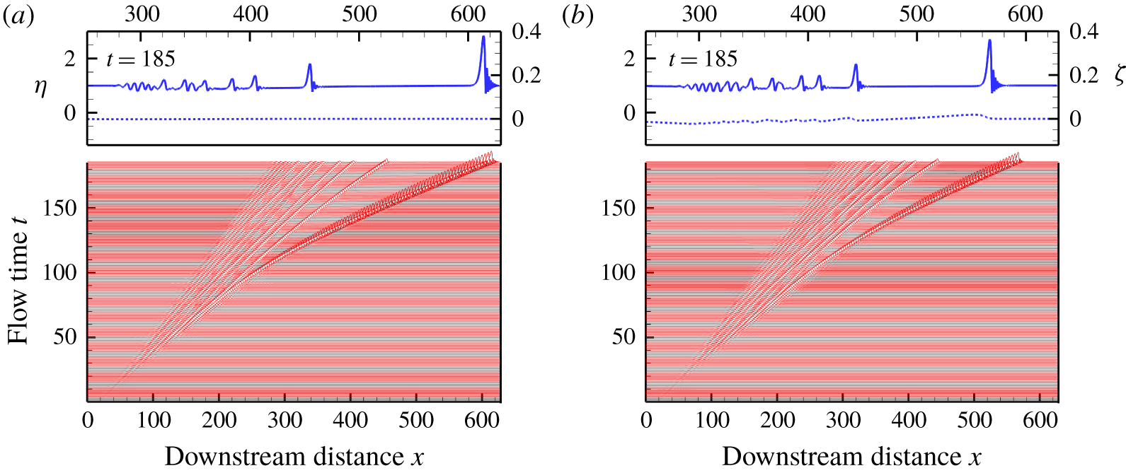
Evolution of the initial imposed wave packet on the air–water free surface for (a)  $St=0.01375$ and (b)
 $St=0.6875$, with
 $Re_{\unicode[STIX]{x1D700}}=We_{\unicode[STIX]{x1D700}}=1.0$,
 $Bi=5.0$,
 $T_{air}=0.8$,
 $M_{a}=0.0$,
 $Pr=13.4733$,
 $\unicode[STIX]{x1D6FC}=8.7460$,
 $\unicode[STIX]{x1D6FD}=3.9929$ and
 $\unicode[STIX]{x1D712}=0.0798$. The solid lines indicate the position of the air–water free surface and the dashed lines show the topography of the ice–water interface.

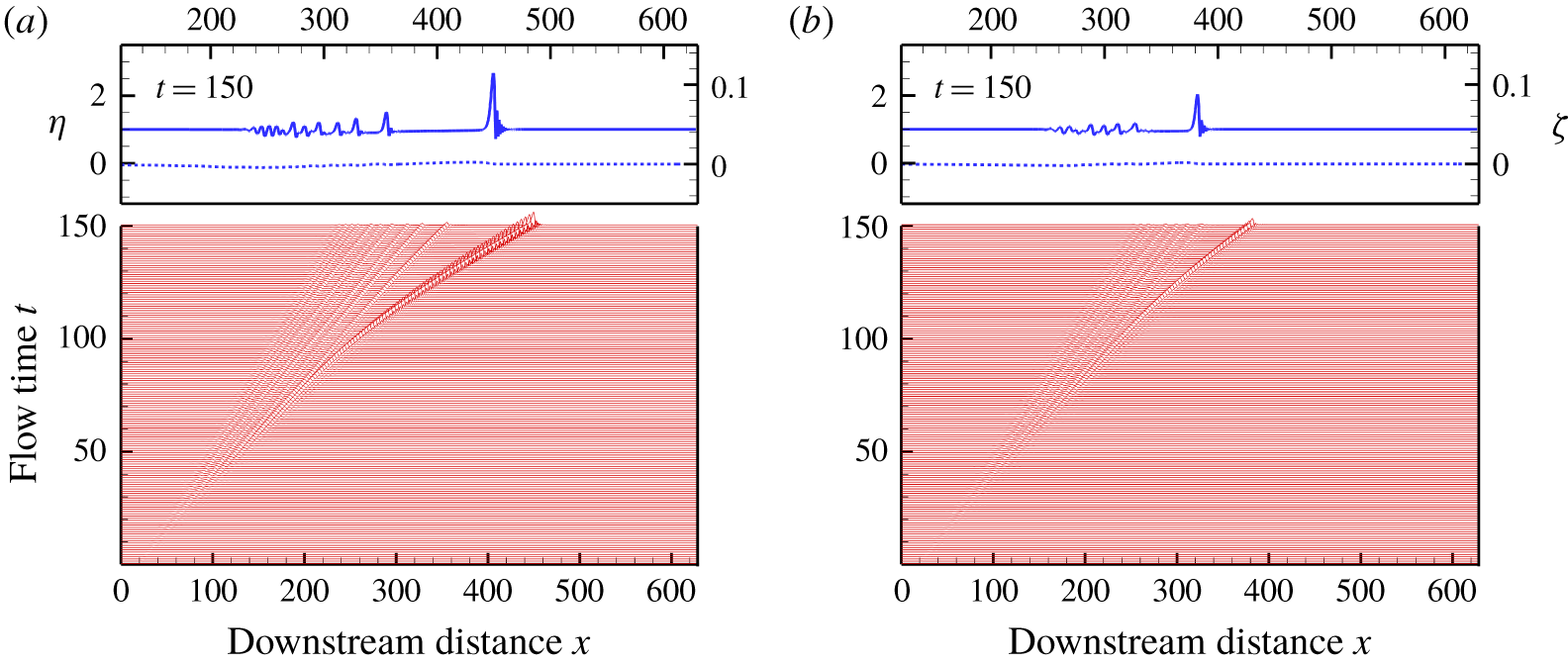
Evolution of the initial imposed wave packet on the air–water free surface for (a)  $M_{a}=0.0$ and (b)
 $M_{a}=1.0$, with
 $Re_{\unicode[STIX]{x1D700}}=We_{\unicode[STIX]{x1D700}}=1.0$,
 $St=0.0687$,
 $Bi=5.0$,
 $T_{air}=0.8$,
 $Pr=13.4733$,
 $\unicode[STIX]{x1D6FC}=8.7460$,
 $\unicode[STIX]{x1D6FD}=3.9929$ and
 $\unicode[STIX]{x1D712}=0.0798$. The solid lines indicate the position of the air–water free surface and the dashed lines show the topography of the ice–water interface.

In figure 14 we show the evolution of the initially imposed wave packet with the different values of  $St$. While it is propagated downstream, the initially imposed wave packet disperses into several interfacial waves. The front wave, which travels with the fastest celerity, separates from the wave packets. It develops into an asymmetrical solitary-like waveform, which is similar to the
 $\unicode[STIX]{x1D6FE}^{1}$ wave shown in figure 9(b). Comparing figures 14(a) and 14(b) show that the development of the front solitary-like wave is delayed slightly due to the increasing Stefan number
 $St$. This again indicates that the phase transition acts to inhibit the dispersion of the system, which is coincident with the conclusion presented in § 4.2. The role of the thermocapillary effect on the dispersion of the initially imposed wave packet is illustrated in figure 15. Comparing figures 15(a) and 15(b) show that the development of the initially imposed wave packet with
 $M_{a}=1.0$ is distinctively slower than that with
 $M_{a}=0.0$. The corresponding wave celerity of the front solitary-like wave with
 $M_{a}=1.0$ is degraded. On the other side, for the small ripples, which are maintained at the rear of the wave system, the wave celerity with
 $M_{a}=1.0$ is faster than that with
 $M_{a}=0.0$. These satisfactorily agree with the results of the steady travelling waves analysis in the previous § 4.2, where the thermocapillary effect acts to delay the fast
 $\unicode[STIX]{x1D6FE}^{1}$ waves but accelerate the slow
 $\unicode[STIX]{x1D6FE}^{-1}$ waves, i.e. it acts to restrain the dispersion of the interfacial wave. This is similar to those presented in previous literature (Peng et al. Reference Peng, Jiang, Zhuge and Zhang2016), where the variation of surface tension is attributed to the interfacial surfactant instead of temperature. The interfacial surfactant can reduce both the amplitude and travelling speed of the solitary-like waveforms. That is, the surfactant acts to weaken the dispersion of the interfacial wave.
5 Direct numerical simulation
Comparison of the thickness of the (a) water layer and (b) ice sheet obtained from DNS versus the IBL equations (2.36)–(2.40). The flow parameters are  $Re_{\unicode[STIX]{x1D700}}=We_{\unicode[STIX]{x1D700}}=1.0$,
 $St=0.1375$,
 $Bi=5.0$,
 $T_{air}=0.8$,
 $Pr=13.4733$,
 $\unicode[STIX]{x1D6FC}=8.7460$,
 $\unicode[STIX]{x1D6FD}=3.9929$,
 $\unicode[STIX]{x1D712}=0.0798$,
 $M_{a}=0.0$ and
 $k=0.11$.

In this section we present direct numerical simulations of the original set of (2.1)–(2.15) based on our in-house code (Yang et al. Reference Yang, Jiang, Hu and Peng2018), which is extended based on the marker and cell (MAC) method. The equations governing the fluid motion and temperature distribution are discretized on a staggered grid fixed on a physical space. Corresponding spatial step sizes along the  $x$-direction and
 $y$-direction are
 $\unicode[STIX]{x0394}x=0.005$ and
 $\unicode[STIX]{x0394}y=0.001$, respectively. The time interval is set to be
 $\unicode[STIX]{x0394}t=10^{-5}$. The interfacial boundary conditions at the air–water free surface and ice–water interface are treated by the donor cell method. The displacements of both the air–water free surface and ice–water interface are tracked accurately and checked according to the integral constraint equation (C 6), which represents the mass conservation of ice and water. The simulation is initialized with the steady Nusselt flow solution expressed in (2.16) and (2.17). A small sinusoidal perturbation is added with a periodic boundary condition being implemented. If the numerical domain is sufficiently large, after a transient evolution, a permanent solitary-like travelling wave can be obtained. This is attributed to the fact that only the fastest travelling waves survive the coarsening process, which occurs in the transient stage (Shkadov & Sisoev Reference Shkadov and Sisoev2004; Samanta et al. Reference Samanta, Ruyer-Quil and Goyeau2011). In figure 16 the local thickness of the water film
 $h_{wt}$ and the ice sheet
 $h_{ice}$ corresponding to the travelling wave obtained from DNS is compared to the results of the IBL equations (2.36)–(2.40). The wavenumber is
 $k=0.11$, and the thermocapillary effect is neglected by letting
 $M_{a}=0.0$. An excellent agreement is achieved for both the solitary waves of the water layer and the surface morphology of the ice layer. It underlines the accuracy of the IBL model presented in § 2.2. However, the IBL model seems to overestimate the amplitude of the capillary wave preceding the hump of the solitary wave. The corresponding displacement of the ice sheet is a little larger than that of the DNS results.
The DNS results of the instantaneous streamline patterns around the depressions that precede the main solitary-like hump without (a)  $St=0.0$, and with phase change at the ice–water interface (b)
 $St=0.1375$ and (c)
 $St=0.6875$. The dashed lines indicate the isocontour of the streamfunction with the value
 $\unicode[STIX]{x1D6F9}=0.0$. See caption in figure 16 for other parameters.

Comparison of the profiles of the (a) streamwise velocity component, (b) pressure and (c) temperature as a function of the  $y$-coordinate at the minimum film thickness. See the caption in figure 16 for other parameters.

In figure 17 we present the instantaneous streamline patterns around the first depression, which precedes the hump. The streamlines, i.e. isocontours of the streamfunction  $\unicode[STIX]{x1D6F9}=\int (u\,\text{d}y-v\,\text{d}x)$, are drawn underneath the elevation of the free surface, which is shown at regularly spaced positive and negative values of
 $\unicode[STIX]{x1D6F9}$ starting from
 $0$. A flow reversal can be found, which extends from the wall up to the air–water free surface (Malamataris, Vlachogiannis & Bontozoglou Reference Malamataris, Vlachogiannis and Bontozoglou2002; Kunugi & Kino Reference Kunugi and Kino2005; Dietze et al. Reference Dietze, Leefken and Kneer2008; Dietze, Al-Sibai & Kneer Reference Dietze, Al-Sibai and Kneer2009; Samanta et al. Reference Samanta, Ruyer-Quil and Goyeau2011). By comparing figures 17(b,c) to 17(a) we can seen that the intensity of the flow reversal phenomenon is increased by the phase transition condition on the ice–water interface as the streamlines are more packed for
 $St=0.6875$ and
 $St=0.1375$ than
 $St=0.0$. This intensification is also observable in figure 18(a), where the streamwise velocity component at the minimum film thickness is shown for different values of
 $St$. For
 $St=0.6875$ and
 $St=0.1375$, the absolute value of the minimum streamwise velocity is more significant than that observed for
 $St=0.0$. According to previous literature (Kunugi & Kino Reference Kunugi and Kino2005; Samanta et al. Reference Samanta, Ruyer-Quil and Goyeau2011), this can result in the improvement of heat and mass transfer at both the ice–water interface and the air–water free surface. Moreover, due to the presence of phase transition, in figure 17 we can see that the structure of the streamlines near the ice–water interface for
 $St=0.1375$ and
 $St=0.6875$ are different from those for
 $St=0.0$. This indicates the effect of phase transition on the flow field near the ice–water interface, which is also intensified as
 $St$ increases since the flow velocity at the ice–water interface is proportional to
 $St$, as shown in (2.12), although the no-slip condition, shown in (2.14), is applied. In figure 18(a) it may be observed that the IBL model tends to overestimate the streamwise velocity at the free surface slightly. The maximum/minimum of the streamwise velocity component is not reached at the air–water free surface for the DNS results. This is different from those obtained from the IBL model, where the assumption of a parabolic velocity profile is implied, and the maximal/minimal streamwise velocity is located at the air–water free surface. In figure 18(b,c) we present the profiles of the pressure and temperature along the minimum film thickness. Although there are deviations in the velocity, temperature and pressure between the DNS and the IBL results, the IBL model can qualitatively well capture the kinematics of the flow.
6 Conclusions
This investigation addresses the spatio-temporal stability of a water film falling down an inclined ice sheet. Based on the integral-boundary-layer theory, a set of nonlinear coupled evolution equations has been developed for the local flow rate  $q(x,t)$, the local thickness of the water film
 $h_{wt}(x,t)$ and ice sheet
 $h_{ice}(x,t)$, and the temperature gradient on both sides of the ice–water interface
 $g_{wt}(x,t)$ and
 $g_{ice}(x,t)$, respectively. The linear instability characteristic of the system is examined by using the normal mode analysis and comparing the results with the Orr–Sommerfeld equations. A convincing agreement has been found. The results show that the long-wavelength perturbations are suppressed due to the presence of the phase transition. The thermocapillary effect, which can subserve the stabilizing role of both phase transition (stabilizing long-wave perturbation) and surface tension (stabilizing short-wave perturbation), plays a stabilizing role in the flow.
In the nonlinear regime the steady travelling waves are considered. It is confirmed that a stable solution with finite amplitude can be obtained if the perturbation wavenumber is smaller than the cut-off value  $k_{cu}$. The thermocapillary effect contributes to suppress the amplitude of the primary wave families, and weaken the dispersion of the system as well. The slowest
 $\unicode[STIX]{x1D6FE}^{-1}$ wave can be accelerated, whereas the fastest
 $\unicode[STIX]{x1D6FE}^{1}$ wave can be decelerated. Similar to the thermocapillary effect, the phase transition also has an inhibitory effect on the dispersion of the system. If the phase transition is enforced, the deformation of the ice–water interface is enlarged, and both the
 $\unicode[STIX]{x1D6FE}^{-1}$ and
 $\unicode[STIX]{x1D6FE}^{1}$ waves are accelerated slightly. Moreover, the nonlinear evolution equations are solved numerically. The accuracy of the reduced nonlinear evolution equations (2.36)–(2.40) based on the IBL theory has been verified through comparison with the solitary-like travelling wave obtained by DNS of the Navier–Stokes equations with periodic boundary conditions. The results suggest that the reduced models can capture the wave shape, amplitude, flow velocity and temperature distribution satisfactorily.
Acknowledgements
The final manuscript benefits from comments and suggestions provided by the referees. In particular, we are indebted to a referee whose comments and questions have enriched the contents of the paper. This work was supported in part by the NSFC under grant no. 11672159.
Declaration of interests
The authors report no conflict of interest.
Appendix A. Equations for linear stability analysis
Substituting the normal modes defined in (3.1) into (2.36)–(2.40) and linearize for  $(Q,H_{wt},H_{ice},G_{wt},G_{ice})\rightarrow 0$ yields
 $$\begin{eqnarray}\displaystyle & \displaystyle c(H_{wt}+(1-\unicode[STIX]{x1D712})H_{ice})=Q, & \displaystyle\end{eqnarray}$$
 $$\begin{eqnarray}\displaystyle & \displaystyle c\frac{Re_{\unicode[STIX]{x1D700}}Pr}{St}H_{ice}=\frac{\text{i}}{k}(\unicode[STIX]{x1D6FD}G_{ice}-G_{wt}), & \displaystyle\end{eqnarray}$$
 $$\begin{eqnarray}\displaystyle cQ & = & \displaystyle k^{2}\frac{H_{ice}+H_{wt}}{We_{\unicode[STIX]{x1D700}}}+\frac{1}{Re_{\unicode[STIX]{x1D700}}}\left(\frac{6\text{i}H_{wt}}{k}-\frac{3\text{i}Q}{k}\right)+\left(\frac{8}{5}Q-\frac{8}{15}H_{wt}\right)\nonumber\\ \displaystyle & & \displaystyle -\,M_{a}\left(\frac{\text{i}k}{30}-\frac{3}{2Re_{\unicode[STIX]{x1D700}}}\right)\left(\frac{G_{wt}}{(2+Bi)}+\frac{2BiT_{air}H_{wt}}{(2+Bi)(1+Bi)}\right),\end{eqnarray}$$
 $$\begin{eqnarray}\displaystyle c\left(G_{wt}+\frac{4Bi(3+Bi)T_{air}H_{wt}}{(1+Bi)(4+Bi)}\right) & = & \displaystyle \frac{BiT_{air}}{(1+Bi)(4+Bi)}\left(\frac{\left(50+7Bi\right)}{10}-\frac{12\text{i}Bi}{kRe_{\unicode[STIX]{x1D700}}Pr}\right)H_{wt}\nonumber\\ \displaystyle & & \displaystyle +\,\left(\frac{(32+7Bi)}{10(4+Bi)}-\frac{12\text{i}(1+Bi)}{kRe_{\unicode[STIX]{x1D700}}Pr(4+Bi)}\right)G_{wt}\nonumber\\ \displaystyle & & \displaystyle -\,\frac{\text{i}kBiT_{air}M_{a}}{8(4+Bi)(1+Bi)}\left(G_{wt}+\frac{2BiT_{air}}{1+Bi}H_{wt}\right)\nonumber\\ \displaystyle & & \displaystyle +\,\frac{15Bi(2+Bi)T_{air}}{4(4+Bi)(1+Bi)}Q,\end{eqnarray}$$
 $$\begin{eqnarray}\displaystyle cG_{ice} & = & \displaystyle 4c\frac{Bi^{2}T_{air}^{2}}{\unicode[STIX]{x1D6FD}^{2}(Bi+1)^{2}(T_{air}-1)}H_{ice}+\frac{12\text{i}\unicode[STIX]{x1D6FC}}{kRe_{\unicode[STIX]{x1D700}}Pr}\frac{Bi^{4}T_{air}^{4}}{\unicode[STIX]{x1D6FD}^{4}(1+Bi)^{4}(T_{air}-1)^{3}}H_{ice}\nonumber\\ \displaystyle & & \displaystyle -\,\frac{12\text{i}\unicode[STIX]{x1D6FC}}{kRe_{\unicode[STIX]{x1D700}}Pr}\frac{Bi^{2}T_{air}^{2}}{\unicode[STIX]{x1D6FD}^{2}(1+Bi)^{2}(T_{air}-1)^{2}}G_{ice}.\end{eqnarray}$$
According to (A 1)–(A 5), a generalized complex eigenvalue system can be derived, which can be solved using the software package MATLAB based on the QZ algorithm.
Appendix B. Long-wavelength instability analysis
We assume  $M_{a}=0$ and substitute (3.2) into (A 1)–(A 5). Then, the items with the same order of
 $k$ are equated separately. For the zero-order solution, the first- and higher-order terms in
 $k$ are ignored. Then we have
 $$\begin{eqnarray}\displaystyle & \displaystyle Q_{0}=2H_{wt,0}, & \displaystyle\end{eqnarray}$$
 $$\begin{eqnarray}\displaystyle & \displaystyle H_{ice,0}=-\frac{\unicode[STIX]{x1D6FD}(T_{air}-1)}{T_{air}}H_{wt,0}, & \displaystyle\end{eqnarray}$$
 $$\begin{eqnarray}\displaystyle & \displaystyle G_{wt,0}=-\frac{Bi^{2}T_{air}}{(1+Bi)^{2}}H_{wt,0}, & \displaystyle\end{eqnarray}$$
 $$\begin{eqnarray}\displaystyle & \displaystyle G_{ice,0}=-\frac{Bi^{2}T_{air}}{\unicode[STIX]{x1D6FD}(1+Bi)^{2}}H_{wt,0}, & \displaystyle\end{eqnarray}$$
 $$\begin{eqnarray}\displaystyle & \displaystyle c_{0}=\frac{2T_{air}}{(T_{air}-\unicode[STIX]{x1D6FD}(1-\unicode[STIX]{x1D712})(T_{air}-1))}. & \displaystyle\end{eqnarray}$$
Considering all the first-order terms of  $k$, then we have
 $$\begin{eqnarray}\displaystyle & \displaystyle c_{1}\frac{Q_{0}}{c_{0}}+c_{0}(H_{wt,1}+(1-\unicode[STIX]{x1D712})H_{ice,1})-Q_{1}=0, & \displaystyle\end{eqnarray}$$
 $$\begin{eqnarray}\displaystyle & \displaystyle \text{i}\unicode[STIX]{x1D6FD}G_{ice,1}-\text{i}G_{wt,1}-c_{0}\frac{Re_{\unicode[STIX]{x1D700}}Pr}{St}H_{ice,0}=0, & \displaystyle\end{eqnarray}$$
 $$\begin{eqnarray}\displaystyle & \displaystyle \frac{6i}{Re_{\unicode[STIX]{x1D700}}}H_{wt,1}-\frac{3i}{Re_{\unicode[STIX]{x1D700}}}Q_{1}+\frac{8}{5}Q_{0}-\frac{8}{15}H_{wt,0}-c_{0}Q_{0}=0, & \displaystyle\end{eqnarray}$$
 $$\begin{eqnarray}\displaystyle & & \displaystyle c_{0}G_{wt,0}+4c_{0}\frac{Bi(3+Bi)T_{air}}{(1+Bi)(4+Bi)}H_{wt,0}-\frac{Bi(50+7Bi)T_{air}}{10(1+Bi)(4+Bi)}H_{wt,0}\nonumber\\ \displaystyle & & \displaystyle \quad +\,\frac{12\text{i}}{Re_{\unicode[STIX]{x1D700}}Pr}\frac{Bi^{2}T_{air}}{(1+Bi)(4+Bi)}H_{wt,1}-\frac{(32+7Bi)}{10(4+Bi)}G_{wt,0}\nonumber\\ \displaystyle & & \displaystyle \quad +\,\frac{12i}{Re_{\unicode[STIX]{x1D700}}Pr}\frac{(1+Bi)}{(4+Bi)}G_{wt,1}-\frac{15Bi(2+Bi)T_{air}}{4(4+Bi)(1+Bi)}Q_{0}=0,\end{eqnarray}$$
 $$\begin{eqnarray}\displaystyle & & \displaystyle c_{0}G_{ice,0}+\frac{12\text{i}\unicode[STIX]{x1D6FC}}{Re_{\unicode[STIX]{x1D700}}Pr}\frac{Bi^{2}T_{air}^{2}}{\unicode[STIX]{x1D6FD}^{2}(1+Bi)^{2}(T_{air}-1)^{2}}G_{ice,1}-4c_{0}\frac{Bi^{2}T_{air}^{2}}{\unicode[STIX]{x1D6FD}^{2}(Bi+1)^{2}(T_{air}-1)}H_{ice,0}\nonumber\\ \displaystyle & & \displaystyle \quad -\,\frac{12\text{i}\unicode[STIX]{x1D6FC}}{Re_{\unicode[STIX]{x1D700}}Pr}\frac{Bi^{4}T_{air}^{4}}{\unicode[STIX]{x1D6FD}^{4}(1+Bi)^{4}(T_{air}-1)^{3}}H_{ice,1}=0.\end{eqnarray}$$
From the above equations, the expression of  $c_{1}$ can be derived. By definition,
 $c_{0}$ is a real number indicating marginal stability. Corresponding wave celerity equals
 $c_{0}$. Hence, the system stability is to be determined by the eigenvalue
 $c_{1}$, which turns out to be a pure imaginary number. Then the analytic solution for a perturbation growth rate is obtained as
 $$\begin{eqnarray}\displaystyle \unicode[STIX]{x1D714}_{r} & = & \displaystyle k^{2}\text{Im}(c_{1})\nonumber\\ \displaystyle & = & \displaystyle k^{2}\frac{4Re_{\unicode[STIX]{x1D700}}T_{air}(T_{air}+2\unicode[STIX]{x1D6FD}(1-\unicode[STIX]{x1D712})(T_{air}-1))}{9(T_{air}-\unicode[STIX]{x1D6FD}(1-\unicode[STIX]{x1D712})(T_{air}-1))^{2}}-k^{2}\frac{4Re_{\unicode[STIX]{x1D700}}Pr\unicode[STIX]{x1D6FD}^{2}(1-\unicode[STIX]{x1D712})(1+Bi)^{2}(T_{air}-1)^{2}}{StBi^{2}(T_{air}-\unicode[STIX]{x1D6FD}(1-\unicode[STIX]{x1D712})(T_{air}-1))^{3}}\nonumber\\ \displaystyle & & \displaystyle +\,k^{2}\frac{Re_{\unicode[STIX]{x1D700}}Pr\unicode[STIX]{x1D6FD}(1-\unicode[STIX]{x1D712})(2+Bi)T_{air}(T_{air}-1)}{12(T_{air}-\unicode[STIX]{x1D6FD}(1-\unicode[STIX]{x1D712})\left(T_{air}-1\right))^{3}}\left(\frac{12\unicode[STIX]{x1D6FD}^{2}(1+Bi)^{2}(T_{air}-1)^{2}}{\unicode[STIX]{x1D6FC}T_{air}Bi^{2}(2+Bi)}\right.\nonumber\\ \displaystyle & & \displaystyle +\,\left.\frac{(3Bi-4)T_{air}-5\unicode[STIX]{x1D6FD}(3Bi+4)(1-\unicode[STIX]{x1D712})(T_{air}-1)}{Bi(1+Bi)}\right)+O(k^{3}).\end{eqnarray}$$
Clearly, the flow is linearly unstable with  $\unicode[STIX]{x1D714}_{r}>0$ while stable with
 $\unicode[STIX]{x1D714}_{r}\leqslant 0$.
Appendix C. Equations for steady travelling waves
Substituting  $\unicode[STIX]{x1D709}=k(x-ct)$ into (2.36)–(2.40), we obtain
 $$\begin{eqnarray}\displaystyle & \displaystyle \frac{\unicode[STIX]{x2202}}{\unicode[STIX]{x2202}\unicode[STIX]{x1D709}}(q-ch_{wt}-c(1-\unicode[STIX]{x1D712})h_{ice})=0, & \displaystyle\end{eqnarray}$$
 $$\begin{eqnarray}\displaystyle & \displaystyle \frac{\unicode[STIX]{x2202}h_{ice}}{\unicode[STIX]{x2202}\unicode[STIX]{x1D709}}=\frac{St}{Re_{\unicode[STIX]{x1D700}}Pr}\frac{g_{wt}-\unicode[STIX]{x1D6FD}g_{ice}}{ck}, & \displaystyle\end{eqnarray}$$
 $$\begin{eqnarray}\displaystyle kc\frac{\unicode[STIX]{x2202}q}{\unicode[STIX]{x2202}\unicode[STIX]{x1D709}}+\frac{2h_{wt}}{Re_{\unicode[STIX]{x1D700}}} & = & \displaystyle -k^{3}\frac{h_{wt}}{We_{\unicode[STIX]{x1D700}}}\frac{\unicode[STIX]{x2202}^{3}(h_{ice}+h_{wt})}{\unicode[STIX]{x2202}\unicode[STIX]{x1D709}^{3}}+\frac{1}{Re_{\unicode[STIX]{x1D700}}}\left(\frac{3q}{h_{wt}^{2}}\right)+\frac{3}{2}\frac{M_{a}}{Re_{\unicode[STIX]{x1D700}}}\unicode[STIX]{x1D713}\nonumber\\ \displaystyle & & \displaystyle +\,k\frac{\unicode[STIX]{x2202}}{\unicode[STIX]{x2202}\unicode[STIX]{x1D709}}\left(\frac{6}{5}\frac{q^{2}}{h_{wt}}+\frac{M_{a}^{2}}{120}\unicode[STIX]{x1D713}^{2}h_{wt}^{3}-\frac{M_{a}}{20}q\unicode[STIX]{x1D713}h_{wt}\right),\end{eqnarray}$$
 $$\begin{eqnarray}\displaystyle c\frac{\unicode[STIX]{x2202}g_{wt}}{\unicode[STIX]{x2202}\unicode[STIX]{x1D709}} & = & \displaystyle \left(\frac{3}{20}\frac{(32+7Bih_{wt})}{(4+Bih_{wt})}\frac{q}{h_{wt}}-\frac{M_{a}\unicode[STIX]{x1D713}(4-Bih_{wt})}{40(4+Bih_{wt})}h_{wt}\right)\frac{\unicode[STIX]{x2202}g_{wt}}{\unicode[STIX]{x2202}\unicode[STIX]{x1D709}}\nonumber\\ \displaystyle & & \displaystyle +\,\left(\frac{3}{40}M_{a}\unicode[STIX]{x1D713}\frac{g_{wt}(Bi^{2}h_{wt}^{2}-8)-4BiT_{air}(3+Bih_{wt})}{(2+Bih_{wt})(4+Bih_{wt})}\right.\nonumber\\ \displaystyle & & \displaystyle -\,\left.2c\frac{g_{wt}(8+5Bih_{wt}+Bi^{2}h_{wt}^{2})+Bi(4+Bih_{wt})T_{air}}{(2+Bih_{wt})(4+Bih_{wt})h_{wt}}\right.\nonumber\\ \displaystyle & & \displaystyle +\,\left.\frac{3}{20}\frac{g_{wt}(64+28Bih_{wt}+7Bi^{2}h_{wt}^{2})+36BiT_{air}}{(2+Bih_{wt})(4+Bih_{wt})}\frac{q}{h_{wt}^{2}}\right)\frac{\unicode[STIX]{x2202}h_{wt}}{\unicode[STIX]{x2202}\unicode[STIX]{x1D709}}\nonumber\\ \displaystyle & & \displaystyle +\,\frac{3}{20}\frac{g_{wt}(32+7Bih_{wt})+18BiT_{air}}{(4+Bih_{wt})h_{wt}}\frac{\unicode[STIX]{x2202}q}{\unicode[STIX]{x2202}\unicode[STIX]{x1D709}}\nonumber\\ \displaystyle & & \displaystyle -\,M_{a}\frac{g_{wt}(4-Bih_{wt})+6BiT_{air}}{40(4+Bih_{wt})}h_{wt}\frac{\unicode[STIX]{x2202}\unicode[STIX]{x1D713}}{\unicode[STIX]{x2202}\unicode[STIX]{x1D709}}\nonumber\\ \displaystyle & & \displaystyle -\,\frac{12}{kRe_{\unicode[STIX]{x1D700}}Pr}\left(\frac{Bi(T_{air}-g_{wt}h_{wt})-g_{wt}}{(4+Bih_{wt})h_{wt}^{2}}\right),\end{eqnarray}$$
 $$\begin{eqnarray}c\frac{\unicode[STIX]{x2202}g_{ice}}{\unicode[STIX]{x2202}\unicode[STIX]{x1D709}}=2c\left(\frac{T_{air}-1}{h_{ice}^{2}}-\frac{g_{ice}}{h_{ice}}\right)\frac{\unicode[STIX]{x2202}h_{ice}}{\unicode[STIX]{x2202}\unicode[STIX]{x1D709}}+\frac{12\unicode[STIX]{x1D6FC}}{kRe_{\unicode[STIX]{x1D700}}Pr}\left(\frac{g_{ice}}{h_{ice}^{2}}+\frac{T_{air}-1}{h_{ice}^{3}}\right).\end{eqnarray}$$
Here,  $\unicode[STIX]{x1D713}$ is defined in (2.35). In order to get the periodical steady-state solutions (
 $0\leqslant \unicode[STIX]{x1D709}<2\unicode[STIX]{x03C0}$) of the above system, both an integral and phase condition should be supplemented. Taking into account the choice of scale in this study, we have
 $$\begin{eqnarray}\displaystyle & \displaystyle \frac{1}{2\unicode[STIX]{x03C0}}\int _{0}^{2\unicode[STIX]{x03C0}}[h_{wt}+(1-\unicode[STIX]{x1D712})h_{ice}]\,\text{d}\unicode[STIX]{x1D709}=1.0+(1-\unicode[STIX]{x1D712})\unicode[STIX]{x1D6FF}, & \displaystyle\end{eqnarray}$$
 $$\begin{eqnarray}\displaystyle & \displaystyle h_{wt}(0)=1.0. & \displaystyle\end{eqnarray}$$
Here,  $\unicode[STIX]{x1D6FF}$ indicates the dimensionless ice sheet thickness of the Nusselt uniform film solution. Equation (C 6) denotes that the waves carry the same mass (include the mass of the ice sheet) as the Nusselt uniform film solution of the same periodicity. Therefore, the system is complete, and the Newton–Kantorovich method was adopted to solve it numerically.