1. Introduction
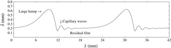
We consider a Newtonian viscous liquid film flowing down a vertical wall due to the action of gravity in a two-dimensional setting. As shown in figure 1 and famously in the seminal experiments of Kapitza (Reference Kapitza1948), the free surface of such a film may deform into a train of solitary pulses, travelling at constant celerity (Pumir, Manneville & Pomeau Reference Pumir, Manneville and Pomeau1983) and displaying a very distinct shape. This consists of a large-amplitude asymmetric main hump in the form of a tear, which is preceded by a number of small ripples, typically designated as ‘capillary waves’, that form on the residual film separating subsequent wave trains. In this manuscript, we set out to answer a number of fundamental questions regarding this generic wave shape. (i) By what mechanism do the precursory ripples form? (ii) How can they travel at the same celerity as the large-amplitude main humps? (iii) Why are they designated as ‘capillary waves’? (iv) What determines their wavelength and number and why do they attenuate in space? First, we provide a short literature overview in order to put the objective of our manuscript into context.
Fully-developed travelling free-surface profile of a vertically-falling wavy liquid film:
 $\mathit{Re}=\tilde{q}/{\it\nu}=15$
,
 $\tilde{f}=16$
Hz,
 ${\it\Lambda}=20.8$
mm,
 $Ka={\it\sigma}/({\it\rho}\,g^{1/3}\,{\it\nu}^{4/3})=509.5$
. Large non-symmetric wave humps form due to the Kapitza instability (Kapitza Reference Kapitza1948) and are preceded by so-called ‘capillary waves’. How do these precursory waves form, how can they keep up with the large humps, why are they called ‘capillary waves’ and what determines their wavelength and number?

Recent reviews on falling liquid films can be found in the monographs of Alekseenko, Nakoryakov & Pokusaev (Reference Alekseenko, Nakoryakov and Pokusaev1994), Chang & Demekhin (Reference Chang and Demekhin2002), and Kalliadasis et al. (Reference Kalliadasis, Ruyer-Quil, Scheid and Velarde2012) and the articles by Chang (Reference Chang1994) and Craster & Matar (Reference Craster and Matar2009). Early works elucidated the linear stability behaviour of this flow (Brooke Benjamin Reference Brooke Benjamin1957; Yih Reference Yih1963), showing the instability to be of the long-wave type at low Reynolds number values (
 $\mathit{Re}=\tilde{q}_{0}/{\it\nu}$
,
 $\tilde{q}_{0}$
and
 ${\it\nu}$
designating the dimensional flow rate per unit width of the unperturbed film and kinematic viscosity, respectively), the stability cutoff being determined by surface tension, expressed through the Kapitza number (
 $Ka={\it\sigma}/({\it\rho}\,g^{1/3}\,{\it\nu}^{4/3})$
,
 ${\it\sigma}$
,
 ${\it\rho}$
and
 $g$
denoting surface tension, density and gravity), and streamwise viscous diffusion (Ruyer-Quil & Manneville Reference Ruyer-Quil and Manneville1998). At large
 $\mathit{Re}$
, short-wave shear modes were shown to occur (Floryan, Davis & Kelly Reference Floryan, Davis and Kelly1987).
Later, numerical simulations based on the Navier–Stokes equations (Salamon, Armstrong & Brown Reference Salamon, Armstrong and Brown1994; Ramaswamy, Chippada & Joo Reference Ramaswamy, Chippada and Joo1996; Miyara Reference Miyara1999; Malamataris, Vlachogiannis & Bontozoglou Reference Malamataris, Vlachogiannis and Bontozoglou2002; Gao, Morley & Dhir Reference Gao, Morley and Dhir2003; Nosoko & Miyara Reference Nosoko and Miyara2004; Trifonov Reference Trifonov2008) and experiments using optical measuring techniques (Liu & Gollub Reference Liu and Gollub1994; Lel et al. Reference Lel, Al-Sibai, Leefken and Renz2005; Tihon et al. Reference Tihon, Serifi, Argyriadi and Bontozoglou2006; Dietze, Al-Sibai & Kneer Reference Dietze, Al-Sibai and Kneer2009) focussed intensively on elucidating the kinematics of surface waves and the flow field they generate. This was complemented by the development of low-dimensional models (Benney Reference Benney1966; Shkadov Reference Shkadov1967; Gjevik Reference Gjevik1970; Ruyer-Quil & Manneville Reference Ruyer-Quil and Manneville2000), which enable physically-consistent simulations on very long domains. Such simulations have represented the full transition of a wavy liquid film from its smooth-surface state at the inlet to interfacial spatio-temporal chaos several meters downstream (Chang et al. Reference Chang, Demekhin, Kalaidin and Ye1996). This evolution is associated with a number of secondary instabilities (Liu, Paul & Gollub Reference Liu, Paul and Gollub1993) as well as interaction and coalescence events between nonlinear surface waves (Malamataris et al. Reference Malamataris, Vlachogiannis and Bontozoglou2002; Pradas, Tseluiko & Kalliadasis Reference Pradas, Tseluiko and Kalliadasis2011). For brevity, we have focused here on two-dimensional studies and merely point out a number of works devoted to the more complicated three-dimensional problem (Joo & Davis Reference Joo and Davis1992; Chang, Demekhin & Kopelevich Reference Chang, Demekhin and Kopelevich1993; Park & Nosoko Reference Park and Nosoko2003; Demekhin et al. Reference Demekhin, Kalaidin, Kalliadasis and Vlaskin2007a ,Reference Demekhin, Kalaidin, Kalliadasis and Vlaskin b , Reference Demekhin, Kalaidin, Kalliadasis and Vlaskin2010; Dietze et al. Reference Dietze, Rohlfs, Nährich, Kneer and Scheid2014; Kofman, Mergui & Ruyer-Qui Reference Kofman, Mergui and Ruyer-Qui2014).
In reviewing the above literature, we have found that questions (i)–(iv), relating to precursory capillary waves on falling liquid films, have, to the best of our knowledge, not been answered. Meanwhile, capillary waves play an important role for the dynamics of these wavy flows and a number of works have highlighted this point. For instance, Malamataris et al. (Reference Malamataris, Vlachogiannis and Bontozoglou2002) have shown that capillary waves may prevent the coalescence of neighbouring large humps of moderately disparate amplitude and Pradas et al. (Reference Pradas, Kalliadasis, Nguyen and Bontozoglou2013) discovered that self-sustained oscillations between large humps of same amplitude may occur when the latter are initially placed at a short distance from one another. Understanding how capillary waves form on wavy falling liquid films and under what circumstances they are most pronounced and greatest in number, may help to elucidate the mechanisms underlying such interactions.
On the other hand, capillary waves generate adverse pressure gradients sufficiently strong to overcome gravity and cause local flow reversal. This was, in principle, already conjectured by Kapitza (Reference Kapitza1948) based on his low-dimensional model and later confirmed by simulations based on the Navier–Stokes equations (Salamon et al. Reference Salamon, Armstrong and Brown1994; Miyara Reference Miyara1999; Malamataris et al. Reference Malamataris, Vlachogiannis and Bontozoglou2002), while the governing mechanism was elucidated by Dietze, Leefken & Kneer (Reference Dietze, Leefken and Kneer2008) and experimental proof was provided by Tihon et al. (Reference Tihon, Serifi, Argyriadi and Bontozoglou2006) and Dietze et al. (Reference Dietze, Al-Sibai and Kneer2009). Meanwhile, Malamataris & Balakotaiah (Reference Malamataris and Balakotaiah2008) showed the existence of multiple flow-reversal regions when several strongly-pronounced capillary waves are present and Dietze et al. (Reference Dietze, Rohlfs, Nährich, Kneer and Scheid2014) identified regions of three-dimensional flow reversal. More recently, Doro & Aidun (Reference Doro and Aidun2013), confirmed by direct numerical simulation (DNS) that flow reversal may also form for sinusoidal surface waves. The authors deduce from this that backflow ‘is not dependent on the presence of capillary waves’. However, the wavelength of their sinusoidal waves is short and not very far from that of typical capillary ripples preceding the asymmetric large hump in figure 1. By understanding the nature of capillary waves on falling liquid films, our manuscript will help to establish whether it is necessary to distinguish these two wave types. Finally, a phase diagram for the onset of flow reversal was recently constructed by Rohlfs & Scheid (Reference Rohlfs and Scheid2015). Bearing in mind the controlling relevance of capillary waves for the onset of flow reversal, the current manuscript may help to provide a physical basis for such correlations.
In summary, despite a number of studies focussing on the effects of capillary waves on falling liquid films, the mechanisms governing their inception, growth and final state as well as the matching of their celerity to that of the large humps, i.e. issues raised in (i)–(iv), seem not to have been understood yet. Nonetheless, a number of interesting indications toward answering these questions can be found in the literature. For instance, Ruyer-Quil & Manneville (Reference Ruyer-Quil and Manneville2000), based on their weighted-residual integral boundary-layer (WRIBL) model, found that streamwise viscous diffusion plays an important role in shaping capillary waves. Also, two intriguing remarks were made by Chang (Reference Chang1994), who, referring to the wavelength of capillary waves, suggested ‘These humps have steep fronts which are relaxed by a series of front-running bow waves whose wavelength is close to the monochromatic waves at inception’ and ‘the bow waves have a wavenumber close to the neutral wavenumber
 ${\it\alpha}_{0}$
which is in excellent agreement with experimental observation.’ A fundamental question then is whether the wavelength of the ‘bow waves’ is smaller or greater than the neutral stability cutoff, i.e. whether they are stable or unstable in terms of the primary Kapitza instability. In § 5, we provide an answer to this question. On a more general note, the wave profile in figure 1 is distinctly reminiscent of ripples forming around objects travelling on deep water. By elucidating the underlying mechanisms of capillary waves on falling liquid films, our manuscript will help judge if these two situations are indeed comparable.
The manuscript is structured as follows. In the first part, § 2, we discuss the mechanics of single-peaked surface waves occurring on an initially smooth falling liquid film due to the Kapitza instability. Such waves appear at low
 $\mathit{Re}$
and can be described with the so-called Benney equation (Benney Reference Benney1966; Gjevik Reference Gjevik1970), which we use to obtain analytic expressions for growth rate and celerity contributions resulting from different physical effects, linking the latter to the shape of the free surface (through the film thickness
 ${\it\delta}$
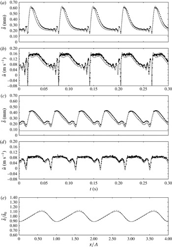
and its derivatives). This part complements the qualitative description of the primary-instability mechanism in Kalliadasis et al. (Reference Kalliadasis, Ruyer-Quil, Scheid and Velarde2012). It will serve in the second part of the manuscript, §§ 3–5 devoted to the precursory capillary waves, which evolve from single-peaked solutions once the main hump amplitude becomes large. In part two, we use DNS of the Navier–Stokes equations, combined with the physical insight gained in the first part, to answer questions (i)–(iii) based on the flow conditions shown in figure 1 (which are outside the validity domain of the Benney equation). In the last part, § 6, we use the low-dimensional WRIBL model of Ruyer-Quil & Manneville (Reference Ruyer-Quil and Manneville2000) to perform extensive parameter variations and answer question (iv). In the conclusion, § 7, we summarize the principal results of the manuscript by succinctly answering the four questions we have posed at the onset. Appendix A contains two figures showing additional simulation data, which will be relevant in § 3, and a third figure validating all employed simulation methods (based on the Benney, integral boundary layer, and Navier–Stokes equations, respectively) with experiments of Dietze et al. (Reference Dietze, Al-Sibai and Kneer2009). Also, the coefficients of the second-order Benney equation, which is used in § 2, are written out there.
2. Mechanics of single-peaked Kapitza waves
The occurrence of capillary waves on falling liquid films is inherently linked to conditions in the large humps that they precede. In fact, capillary waves evolve from single-peaked travelling wave solutions (consisting of a single hump and trough) once the amplitude of the main hump becomes large. Consequently, we start in this section by explaining the mechanics of single-peaked surface waves, developing on an initially smooth falling liquid film due to the Kapitza instability. In this limit, surface waves are of moderate amplitude and long length and can be described by asymptotic expansion (Oron, Davis & Bankoff Reference Oron, Davis and Bankoff1997) around the smooth film base flow, which results from an equilibrium between gravity and viscous stresses and is given by the dimensionless streamwise velocity profile:
 $$\begin{eqnarray}u_{0}(y)=3\left[y-\frac{y^{2}}{2}\right]\end{eqnarray}$$
(
 $y$
is the wall normal or crosswise coordinate), where the length scale was chosen as the unperturbed film thickness
 $L=\tilde{{\it\delta}}_{0}=(3\,\tilde{q}_{0}\,({\it\mu}/{\it\rho})/g)^{1/3}$
(
 ${\it\mu}$
denotes dynamic viscosity and
 $\tilde{q}_{0}$
dimensional flow rate per unit width), and the velocity scales as the corresponding mean velocity
 $U=\tilde{q}_{0}/\tilde{{\it\delta}}_{0}$
(the time scale is
 $L/U$
). Asymptotic expansion truncated at first order in the long-wave parameter
 ${\it\epsilon}=\tilde{{\it\delta}}_{0}/{\it\Lambda}$
(where
 ${\it\Lambda}$
denotes the wavelength) yields the so-called Benney equation (Benney Reference Benney1966; Gjevik Reference Gjevik1970):
 $$\begin{eqnarray}\partial _{t}{\it\delta}=-3{\it\delta}^{2}\,\partial _{x}{\it\delta}-\frac{3}{5}\mathit{Re}[12{\it\delta}^{5}\,(\partial _{x}{\it\delta})^{2}+2{\it\delta}^{6}\,\partial _{xx}{\it\delta}]-\frac{1}{\mathit{Bo}}{\it\delta}^{2}[3\,\partial _{x}{\it\delta}\partial _{xxx}{\it\delta}+{\it\delta}\partial _{xxxx}{\it\delta}],\end{eqnarray}$$
written here in non-conservative form, which describes the evolution of the film thickness
 ${\it\delta}$
. On the right-hand side of (2.2), the first term expresses the balance between gravity and crosswise viscous diffusion, the second, scaled by the Reynolds number
 $\mathit{Re}=\tilde{q}_{0}\,{\it\rho}/{\it\mu}$
, the effect of inertia and the third, scaled by the inverse Bond number
 $\mathit{Bo}=3/(\mathit{Re}\mathit{We})={\it\rho}\,g\,L^{2}/{\it\sigma}$
(where
 $\mathit{We}={\it\sigma}/({\it\rho}\,U^{2}\,L)$
denotes the Weber number), the effect of surface tension
 ${\it\sigma}$
.
In addition, by taking into account the integral continuity equation:
 $$\begin{eqnarray}\partial _{t}{\it\delta}+\partial _{x}q=0\end{eqnarray}$$
(derived using the kinematic condition
 $v|_{y={\it\delta}}=\text{d}{\it\delta}/\text{d}t$
), a relation for the celerity of travelling waves (
 $\text{d}{\it\delta}=0$
) can be obtained:
 $$\begin{eqnarray}c=\partial _{{\it\delta}}q.\end{eqnarray}$$
Employing the flow rate to film-thickness relation underlying (2.2):
 $$\begin{eqnarray}q={\it\delta}^{3}\left[1+\frac{6}{5}\mathit{Re}{\it\delta}^{3}\partial _{x}{\it\delta}+\frac{1}{\mathit{Bo}}\,\partial _{xxx}{\it\delta}\right],\end{eqnarray}$$
one then obtains from (2.4):
 $$\begin{eqnarray}c=3{\it\delta}^{2}+\frac{36}{5}\mathit{Re}{\it\delta}^{5}\partial _{x}{\it\delta}+\frac{3}{\mathit{Bo}}{\it\delta}^{2}\partial _{xxx}{\it\delta}+\frac{{\it\Psi}}{\partial _{x}{\it\delta}},\end{eqnarray}$$
with
 $$\begin{eqnarray}{\it\Psi}=\frac{6}{5}\mathit{Re}{\it\delta}^{6}\partial _{xx}{\it\delta}+\frac{1}{\mathit{Bo}}{\it\delta}^{3}\partial _{xxxx}{\it\delta}.\end{eqnarray}$$
Equations (2.2) and (2.6a
) will be used to highlight different mechanisms governing the growth rate and celerity of single-peaked waves. We will loosely refer to
 $\partial _{t}{\it\delta}$
as the ‘growth rate’, although the proper form of a growth rate requires
 ${\it\delta}^{-1}\partial _{t}{\it\delta}$
. Also, the local ‘growth rate’
 $\partial _{t}{\it\delta}$
is different from the total ‘growth rate’
 $\text{d}{\it\delta}/\text{d}t=\partial _{t}{\it\delta}+u|_{{\it\delta}}\partial _{x}{\it\delta}$
, but the dynamics are contained in
 $\partial _{t}{\it\delta}$
and
 $\partial _{t}{\it\delta}=\text{d}{\it\delta}/\text{d}t$
at the wave extrema.
In the limit of inertialess flow without surface tension (
 $\mathit{Re}\rightarrow 0$
,
 $1/\mathit{Bo}\rightarrow 0$
):
 $$\begin{eqnarray}\partial _{t}{\it\delta}=-3{\it\delta}^{2}\,\partial _{x}{\it\delta},\quad c=3{\it\delta}^{2},\quad q={\it\delta}^{3},\end{eqnarray}$$
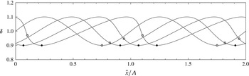
which describes so-called kinematic waves (Brooke Benjamin Reference Brooke Benjamin1957) depicted in figure 2 for a representative set of parameter values. We may discern two key features from this (see Kalliadasis et al.
Reference Kalliadasis, Ruyer-Quil, Scheid and Velarde2012): (i) The wave humps travel faster than the troughs (
 $c=3{\it\delta}^{2}$
), leading to a compression of the wave fronts and an elongation of the wave tails into a non-symmetric waveforms. This development is never arrested, eventually leading to a shock (not shown in the graph); (ii) the growth rate at the extrema is zero and the wave amplitude imposed by the initial condition remains unchanged over time. From a physical point of view, kinematic waves occur because the flow rate
 $q$
is greater in thicker than in thinner regions of the film, which, by mass conservation, drains regions of increasing and inflates regions of decreasing film thickness.
Kinematic wave governed by (2.7):
 $\tilde{{\it\delta}}_{0}=0.1$
mm,
 $g=9.81$
m s
 $^{-2}$
,
 ${\it\mu}=0.001$
Pa s,
 ${\it\rho}=1000$
kg m
 $^{-3}$
,
 ${\it\Lambda}=100\tilde{{\it\delta}}_{0}$
. Starting from a harmonic initial condition, the wave moves from left to right at times
 $\tilde{t}=0$
, 0.02, 0.04 and 0.06 s, steepening without growing in amplitude. Filled/open circles mark loci of minimal
 ${\it\delta}/$
maximal
 $\partial _{xx}{\it\delta}$
(at
 $\tilde{t}=0$
, these points coincide).

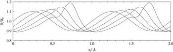
Dynamic wave governed by (2.8a
):
 $\tilde{{\it\delta}}_{0}=0.1$
mm,
 $g=9.81$
m s
 $^{-2}$
,
 ${\it\mu}=0.001$
Pa s,
 ${\it\rho}=1000$
kg m
 $^{-3}$
,
 ${\it\Lambda}=100{\it\delta}_{0}$
. Starting from a harmonic initial condition, the wave moves from left to right at times
 $t=0$
, 0.01, 0.02, 0.03 and 0.04 s, growing in amplitude due to the effect of inertia.

The cause for the growth of Kapitza waves is inertia. For this, we consider (2.2) and (2.5) at finite Reynolds number and in the limit
 $1/\mathit{Bo}\rightarrow 0$
:
 $$\begin{eqnarray}\displaystyle & \partial _{t}{\it\delta}=-3{\it\delta}^{2}\,\partial _{x}{\it\delta}-{\textstyle \frac{3}{5}}\mathit{Re}[12{\it\delta}^{5}\,(\partial _{x}{\it\delta})^{2}+2{\it\delta}^{6}\,\partial _{xx}{\it\delta}], & \displaystyle\end{eqnarray}$$
 $$\begin{eqnarray}\displaystyle & q={\it\delta}^{3}\left[1+{\textstyle \frac{6}{5}}\mathit{Re}{\it\delta}^{3}\partial _{x}{\it\delta}\right]\!. & \displaystyle\end{eqnarray}$$
 $\partial _{xx}{\it\delta}$
in (2.8a
). This causes wave humps, where
 $\partial _{xx}{\it\delta}<0$
, to grow in height and troughs, where
 $\partial _{xx}{\it\delta}>0$
, to grow in depth. The effect is scaled by
 ${\it\delta}^{6}$
so that humps grow faster than troughs deepen. These features are illustrated in figure 3, plotting the solution of (2.8a
) for the same parameters as figure 2. Because (2.8a
) contains no attenuating terms, the amplitude of the waves in figure 3 eventually diverges, which is unphysical.
Mechanically, the effect of inertia can be explained as follows. Lack of it means that flow-rate variations adapt infinitely fast to film-thickness variations. In that case, considering two points either side of and infinitely close to an extremum, e.g. a wave crest, the associated film thicknesses are the same, and consequently, the flow rate in (2.7) does not vary. According to (2.3), the growth rate must thus be null. However, if inertia is present, the film-thickness history, resulting from the passage of surface waves at the two points, must be taken into account. Indeed, the downstream point has just increased its film thickness (as
 $\partial _{x}{\it\delta}<0$
). Considering that the corresponding flow rate needs a finite time to react to this change, its value (2.8b
) is thus slightly too low. Conversely, at the upstream point (where
 $\partial _{x}{\it\delta}<0$
), the flow rate is slightly too high. This leads to a negative
 $\partial _{x}q$
and thus a positive growth rate
 $\partial _{t}{\it\delta}$
at any wave hump. The contrary is true at a wave trough, where the free-surface curvature
 $\partial _{xx}{\it\delta}>0$
. Throughout this manuscript, we will refer to
 $\partial _{xx}{\it\delta}$
as the free-surface curvature although the precise formulation is
 $\partial _{xx}{\it\delta}/(1+\partial _{x}{\it\delta})^{3/2}$
. This is convenient and tenable, as the correction involving
 $\partial _{x}{\it\delta}$
vanishes at extrema, is negligible for long surface waves, and does not influence the sign of the curvature. Meanwhile, the inertia effect in (2.8) is scaled by powers of
 ${\it\delta}$
, because the flow rate adapts to film-thickness variations by way of momentum diffusion in y-direction.
The second term in (2.8a
), although it vanishes at the extrema, does play a role in the wave front and back, where it always (by being proportional to
 $(\partial _{x}{\it\delta})^{2}$
) decreases the growth rate. This again results from the inertia-induced lag (relative to the kinematic waves) of the flow rate in adapting to a time-varying film thickness and, in particular, the increase of lag magnitude with increasing film thickness. In the wave front,
 $\partial _{x}{\it\delta}<0$
and the flow-rate lag is decreasingly negative as
 ${\it\delta}$
decreases, causing a negative growth-rate contribution:
 $\partial _{x}q>0\rightarrow \partial _{t}{\it\delta}<0$
. In the wave back,
 $\partial _{x}{\it\delta}>0$
but the flow-rate lag there is positive and increases with
 ${\it\delta}$
so that once again:
 $\partial _{x}q>0\rightarrow \partial _{t}{\it\delta}<0$
.
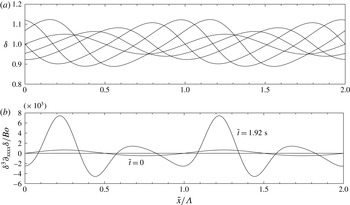
The saturation of Kapitza waves to a finite amplitude is caused by surface tension forces and their effect on the streamwise pressure gradient. For this, we consider the full form of (2.2), the solution of which is shown in figure 4(a) for the same parameters as in figures 2 and 3, additionally setting the surface tension to the value of water
 ${\it\sigma}=0.072$
N m
 $^{-1}$
. This surface tension evidently causes the wave amplitude to saturate, creating a travelling wave of fixed shape in its own reference frame. The arrest of growth at the extrema is caused by the last term in (2.2) and determined by the sign of the fourth derivative
 $\partial _{xxxx}{\it\delta}$
. Figure 4(b) plots this term for the initial (sinusoidal) profile and that of the final travelling wave. We see that
 $\partial _{xxxx}{\it\delta}$
is always negative at the troughs, increasing
 $\partial _{t}{\it\delta}$
according to (2.2), and positive at the humps, decreasing
 $\partial _{t}{\it\delta}$
there.
Physically, this can be explained by considering that
 $\partial _{xxx}{\it\delta}$
imposes the streamwise pressure gradient
 $\partial _{x}p=-\mathit{We}\,\partial _{xxx}{\it\delta}$
through the effect of surface tension forces. Indeed, when moving from a wave trough toward a hump, the free-surface curvature decreases (
 $\partial _{xxx}{\it\delta}<0$
) and surface tension forces create a pressure gradient directed from the hump to the trough, which in simple terms tends to equalize film thickness variations. To be more accurate, the effect of this pressure gradient on the flow rate (2.5) must be considered. A pressure gradient directed counter to the flow will tend to reduce
 $q$
and vice-versa. Spatial flow-rate variations (which through (2.3) impose the local growth rate) can thus be generated by a change in pressure gradient, i.e.
 $\partial _{xx}p=-\mathit{We}\partial _{xxxx}{\it\delta}\neq 0$
. This introduces the fourth film-thickness derivative, which, even for a sinusoidal profile (figure 4
b), is positive at the humps (
 $\partial _{xx}p<0\rightarrow \partial _{x}q>0\rightarrow \partial _{t}{\it\delta}<0$
) and negative at the troughs (
 $\partial _{xx}p>0\rightarrow \partial _{x}q<0\rightarrow \partial _{t}{\it\delta}>0$
). Meanwhile, the effect scales with
 ${\it\delta}^{3}$
in (2.2), so that it is stronger (and increasingly so with increasing
 ${\it\delta}$
) at the humps than at the troughs, nicely balancing the inertia-induced growth disparity between extrema. Physically, this scaling results from the sensitivity of the flow rate (2.5) to the pressure gradient, which accelerates/decelerates the flow over the entire film thickness.
Saturating wave governed by (2.2):
 $\tilde{{\it\delta}}_{0}=0.1$
mm,
 $g=9.81$
m s
 $^{-2}$
,
 ${\it\mu}=0.001$
Pa s,
 ${\it\rho}=1000$
kg m
 $^{-3}$
,
 ${\it\sigma}=0.072$
N m
 $^{-1}$
,
 ${\it\Lambda}=100\tilde{{\it\delta}}_{0}$
,
 $\mathit{Re}=3.27$
. Starting from a harmonic initial condition, the wave moves from left to right at times
 $\tilde{t}=0$
, 0.22, 0.54, 1.07, 1.8 and 1.92 s, growing initially and saturating to a constant amplitude due to the effect of surface tension forces. (a) Film-thickness profile; (b) profile of
 ${\it\delta}^{3}\partial _{xxxx}{\it\delta}/\mathit{Bo}$
in (2.2) evaluated at
 $\tilde{t}=0$
, 1.92 s.

In preparation of the second part of the manuscript, we seek to identify what mechanisms allow the trough and hump of the travelling wave in figure 4(a) to eventually propagate at the same celerity. The local celerity is given by (2.6a
). At the extrema
 $x=x_{E}$
, both
 $\partial _{x}{\it\delta}$
and
 ${\it\Psi}$
tend to zero (
 $\lim _{x\rightarrow x_{E}}({\it\Psi})=0$
follows from requiring a finite celerity), so that l’Hôpital’s rule needs to be applied to the last term in (2.6a
):
 $$\begin{eqnarray}{\it\Xi}=\lim _{x\rightarrow x_{E}}\frac{{\it\Psi}}{\partial _{x}{\it\delta}}=\frac{6}{5}\mathit{Re}{\it\delta}^{6}\frac{\partial _{xxx}{\it\delta}}{\partial _{xx}{\it\delta}}+\frac{1}{\mathit{Bo}}{\it\delta}^{3}\frac{\partial _{xxxxx}{\it\delta}}{\partial _{xx}{\it\delta}},\end{eqnarray}$$
which yields:
 $$\begin{eqnarray}c|_{x=x_{E}}=3{\it\delta}^{2}+\frac{3}{\mathit{Bo}}{\it\delta}^{2}\partial _{xxx}{\it\delta}+{\it\Xi}.\end{eqnarray}$$
Evaluating this relation for the profile at
 $t=1.92$
s in figure 4(a), led to the following observations. The first term of (2.9b
) is proportional to
 ${\it\delta}^{2}$
and causes the wave hump to travel faster than the wave trough. This effect is amplified by the inertial term in (2.9a
) because
 $\partial _{xxx}{\it\delta}<0$
and the free-surface curvature is negative at the hump (
 $\partial _{xx}{\it\delta}<0$
) and positive at the trough (
 $\partial _{xx}{\it\delta}>0$
). Conversely (because
 $\partial _{xxxxx}{\it\delta}>0$
), this change in curvature between hump and trough tends to slow down the former and speed up the latter through the capillary term in (2.9a
). It is thus the effect of surface tension, through the last term in (2.9a
), that arrests the celerity disparity between humps and troughs.
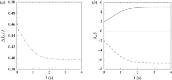
Figure 5 plots the time evolution of the streamwise separation between wave hump and trough from figure 4 as well as the free-surface curvature at these positions. The initial celerity difference between the extrema causes a compression of the wave front (decreasing
 ${\rm\Delta}x_{E}$
) that is at first rapid and subsequently slower and degressive as the celerities converge. In the process, the magnitude of the free-surface curvature increases, whereby
 $|\partial _{xx}{\it\delta}|$
attains a greater value at the trough than at the hump.
Free-surface evolution according to (2.2) as wave hump and trough converge in celerity. (a) Streamwise distance between trough and hump; (b) free-surface curvature at the hump (dashed line) and trough (solid line). Celerity matching is accompanied/generated by a streamwise compression of the hump–trough separation, increasing the curvature magnitudes.

We conclude by discussing the effect of streamwise viscous diffusion, which we will later show to play a role in shaping capillary waves. This effect enters asymptotic expansion at higher order and we must consider the Benney equation truncated at
 ${\it\epsilon}^{2}$
(Lin Reference Lin1974):
 $$\begin{eqnarray}\partial _{t}{\it\delta}={\partial _{t}{\it\delta}}_{(2.2)}-\partial _{x}[D(\partial _{x}{\it\delta})^{2}+E\,\partial _{xx}{\it\delta}+F\,\partial _{xxxx}{\it\delta}+G\,\partial _{x}{\it\delta}\,\partial _{xxx}{\it\delta}+H(\partial _{xx}{\it\delta})^{2}{\it\delta}+I(\partial _{x}{\it\delta})^{2}\partial _{xx}{\it\delta}],\end{eqnarray}$$
where the coefficients
 $D$
to
 $I$
are all functions of
 ${\it\delta}$
and are given in (A 1), whereas the underlying relation for the flow rate is:
 $$\begin{eqnarray}q=q_{(2.5)}+D(\partial _{x}{\it\delta})^{2}+E\,\partial _{xx}{\it\delta}+F\,\partial _{xxxx}{\it\delta}+G\,\partial _{x}{\it\delta}\,\partial _{xxx}{\it\delta}+H(\partial _{xx}{\it\delta})^{2}{\it\delta}+I(\partial _{x}{\it\delta})^{2}\partial _{xx}{\it\delta}.\end{eqnarray}$$
The contributions related to streamwise viscous diffusion are:
 $$\begin{eqnarray}{\partial _{t}{\it\delta}}_{{\it\mu}}=-\partial _{x}[7{\it\delta}^{3}\partial _{x}{\it\delta}^{2}+3{\it\delta}^{4}\partial _{xx}{\it\delta}]\quad \text{and}\quad q_{{\it\mu}}=7{\it\delta}^{3}\partial _{x}{\it\delta}^{2}+3{\it\delta}^{4}\partial _{xx}{\it\delta}.\end{eqnarray}$$
In the first equation, only the term
 $-3{\it\delta}^{4}\partial _{xxx}{\it\delta}$
is non-zero at the extrema and thus the growth rate there is prescribed by the third film-thickness derivative
 $\partial _{xxx}{\it\delta}$
. Physically, this can be understood as follows. At zeroth order, the local instantaneous velocity profile is
 $u=3{\it\delta}y-(3/2)y^{2}$
and so
 $\partial _{xx}u\approx 3y\partial _{xx}{\it\delta}$
. This means that, at a wave hump (
 $\partial _{xx}{\it\delta}<0$
), fluid elements are subjected to an upstream-resulting streamwise viscous stress, while the contrary is true at a wave trough (
 $\partial _{xx}{\it\delta}>0$
). This effect tends to reduce the flow rate at the hump and increase it at the trough (2.12). The corresponding streamwise change in flow rate
 $\partial _{x}q$
is then given by the change in free-surface curvature, i.e.
 $\partial _{xxx}{\it\delta}$
, which is negative at both the wave hump and trough. Consequently, streamwise viscous diffusion increases the growth rate at both extrema
 ${\partial _{t}{\it\delta}}_{{\it\mu}}=-{\partial _{x}q}_{{\it\mu}}>0$
. Of course, for the trough,
 ${\partial _{t}{\it\delta}}_{{\it\mu}}>0$
means that it grows less deep. As opposed to surface tension, the effect of streamwise viscous diffusion is thus ‘non-symmetrical’.
Finally, let us consider how this affects the celerity at the extrema. Differentiating (2.11) with respect to
 ${\it\delta}$
, considering the limit
 $x=x_{E}$
, and retaining only terms related to streamwise viscous diffusion, yields:
 $$\begin{eqnarray}c_{{\it\mu}}|_{x=x_{E}}=26{\it\delta}^{3}\,\partial _{xx}{\it\delta}+3{\it\delta}^{4}\,\frac{\partial _{xxxx}{\it\delta}}{\partial _{xx}{\it\delta}}.\end{eqnarray}$$
It turns out that both terms on the right-hand side of (2.13) counteract the celerity difference between maxima and minima resulting from (2.7). Indeed, the first term is proportional to the free-surface curvature, which tends to slow down the hump (
 $\partial _{xx}{\it\delta}<0$
) and speed up the trough (
 $\partial _{xx}{\it\delta}>0$
). The second term needs to be evaluated numerically. A calculation based on (2.10) for the same parameters as in figure 4 showed that
 $\partial _{xxxx}{\it\delta}>0$
at the hump and
 $\partial _{xxxx}{\it\delta}<0$
at the trough, which tends to further counteract celerity differences.
3. How are capillary waves generated?
Capillary waves evolve from single-peaked wave solutions once the wave amplitude becomes large. This happens at greater Reynolds number values than considered up until now, when the solution of (2.2) diverges due to the strong nonlinearities contained therein (Pumir et al. Reference Pumir, Manneville and Pomeau1983). Consequently, we will base our analysis in §§ 3–5 on DNS of the Navier–Stokes equations using the volume-of-fluid/continuum-surface-force code Gerris (Popinet Reference Popinet2009). Nonetheless, the basic relationships identified in § 2 between governing mechanisms of wave-growth/celerity and free-surface kinematics will help in identifying plausible physical mechanisms surrounding the inception and dynamics of capillary waves, which we will subsequently verify with our DNS data.
Parameters for the DNS in § 3. The Kapitza number
 $Ka={\it\sigma}/({\it\rho}\,g^{1/3}\,{\it\nu}^{4/3})=509.5$
for both cases and ‘
 $\infty$
’ denotes the hydrodynamically developed state. See appendix A for validation of the two simulations with experiments by Dietze et al. (Reference Dietze, Al-Sibai and Kneer2009).

DNS of two representative flow scenarios (table 1) have been performed. These two simulations, cases 1 and 2, have been validated in appendix A with appropriate experiments (Dietze et al.
Reference Dietze, Al-Sibai and Kneer2009; Dietze Reference Dietze2010). They were conducted on a domain of length
 ${\it\Lambda}$
using a periodic boundary condition in the streamwise direction and starting from a sinusoidal film-thickness perturbation about a flat film:
 $$\begin{eqnarray}{\it\delta}|_{t=0}=\bar{{\it\delta}}\,[1+{\it\epsilon}\cos (2{\rm\pi}\,\tilde{x}/{\it\Lambda})],\end{eqnarray}$$
where the mean film thickness
 $\bar{{\it\delta}}$
and the domain length
 ${\it\Lambda}$
represent the actual control parameters, which fix the Reynolds number
 $Re^{\infty }$
and wave frequency
 $f^{\infty }$
of the developed state (denoted by ‘
 $\infty$
’). The perturbation amplitude
 ${\it\epsilon}=0.4$
and the initial streamwise velocity
 $u|_{t=0}=3{\it\delta}|_{t=0}y-(3/2)y^{2}$
. We point out that the use of periodic boundary conditions fixes the volume of the liquid film to a constant throughout the simulation. Thus, it is the Reynolds number
 $\mathit{Re}=({\it\rho}/({\it\Lambda}\,{\it\mu}))\int _{0}^{{\it\Lambda}}\int _{0}^{\tilde{{\it\delta}}}\tilde{u} \,\text{d}{\tilde{y}}\,\text{d}\tilde{x}$
and wave frequency that vary over time, starting from a value set by the initial conditions and converging toward the fully-developed values
 $\mathit{Re}^{\infty }$
and
 $f^{\infty }$
. Though DNS studies showing the time evolution of surface waves have been performed before (Malamataris et al.
Reference Malamataris, Vlachogiannis and Bontozoglou2002; Dietze et al.
Reference Dietze, Leefken and Kneer2008; Doro & Aidun Reference Doro and Aidun2013), these have not focussed on explaining the inception of capillary waves.
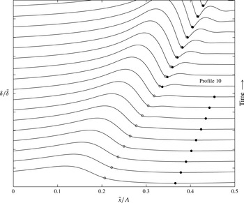
DNS of a vertically falling film:
 $\bar{\tilde{{\it\delta}}}=302~{\rm\mu}$
m,
 $\mathit{Re}^{\infty }=15$
,
 $\tilde{f}^{\infty }=16$
Hz,
 $Ka=509.5$
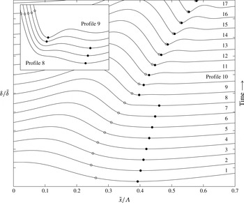
(see appendix A for validation with experiments). Time evolution of the free-surface profile over the timespan
 $t=\tilde{t}/{\it\tau}\in [0.75:0.2:4.15]$
(time scale:
 ${\it\tau}=(H^{3}{\it\rho}/{\it\sigma})^{1/2}$
, with
 $H=1.5$
mm denoting the height of the DNS domain). Profiles in the main graph are represented over the film-thickness interval
 ${\it\delta}/\bar{{\it\delta}}\in [0.4,2.4]$
and those in the blown-up inset over
 ${\it\delta}/\bar{{\it\delta}}\in [0.6,0.9]$
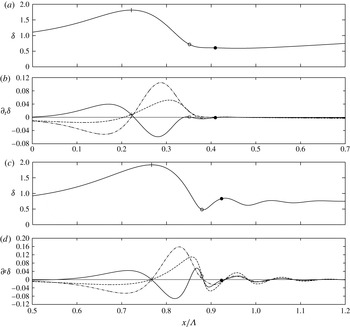
. In the initial stages, as the main wave front steepens, a maximum of free-surface curvature (open circle) is established at its ‘foot’ and not at the global wave trough (filled circle). According to (2.8a
), this locally increases the magnitude of the (negative) growth rate there, eventually producing a new global film-thickness minimum (see evolution between profiles 8 and 9 in inset), and, as a result, the first capillary wave, ‘sandwiched’ between the former and actual global minimum.

The inception of capillary waves is a direct consequence of the primary Kapitza instability discussed in § 2 and the non-symmetric surface waves it generates. This is shown for case 1 in figure 6, depicting free-surface profiles evolving over time during growth of a large wave hump (see figure 8 for later times). The earliest, i.e. bottommost, profile displays a large asymmetric wave hump preceded by a single wave trough. It is similar to those plotted in figure 4(a) as it exhibits a single maximum and a single minimum. This remains so over roughly the next five profiles while growth of the wave hump increasingly compresses/steepens the wave front. However, from the eighth profile onwards, a new local wave trough, which we will call ‘capillary trough’, develops near the foot of the wave front and increases in depth as time goes on, eventually undercutting the erstwhile global wave trough. This is highlighted by the inset in figure 6, showing a blown-up view of the free-surface profile in finer time resolution.
Profiles of the free-surface curvature
 $\partial _{xx}{\it\delta}$
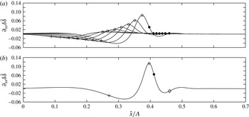
corresponding to the third to ninth (a) and the tenth (b) profile in figure 6. The locus of the wave hump is marked with a plus sign, that of the wave trough with a filled circle, and that of the precursory capillary hump by a diamond (b), while the open circle marks the curvature maximum. (a) Shows that this curvature maximum occurs between the main hump and trough, causing the inertia-driven inception of a capillary trough at the foot of the wave front (figure 6). Because the depth of this trough increases, the associated curvature magnitude becomes very large (b).

The underlying mechanism can be inferred as a first approximation by going back to the growth-rate expression (2.2) (see discussion surrounding (3.2) for confirmation with DNS), where we had established the importance of free-surface curvature
 $\partial _{xx}{\it\delta}$
in driving inertia-induced growth. According to this, we conjecture that the capillary trough develops within the wave front of the main hump due to large positive curvature and associated inertia-induced negative growth there. The locus of maximal
 $\partial _{xx}{\it\delta}$
is highlighted with an open circle for each profile in figure 6. Interestingly, in the early stages, it does not correspond to the global film-thickness minimum (filled circles). Rather, the maximum of
 $\partial _{xx}{\it\delta}$
occurs near the foot of the wave front, close to where the capillary trough eventually develops (onwards from profile 8). Growth in depth of this local trough further increases the related free-surface curvature and thus amplifies itself, causing it to become the new global film-thickness minimum from the ninth profile onwards. This self-amplification of the growth mechanism is demonstrated in figure 7, representing free-surface curvature profiles corresponding to the third to ninth (a) and the tenth (b) film-thickness profiles in figure 6. Indeed, the curvature maximum therein (open circle) significantly increases during the development of the capillary trough (filled circle).
We point out that the capillary trough does not occur exactly at the free-surface curvature maximum, as can be seen in figures 6 and 7. This is because the curvature maximum appears within the wave front, where
 $\partial _{x}{\it\delta}<0$
and the kinematic growth-rate contribution (2.7) is positive (and dominates the slope-related inertial contribution in (2.8a
)). Consequently, the total (negative) growth-rate maximum is moved toward a position of lesser
 $|\partial _{x}{\it\delta}|$
, i.e. slightly downstream. This kinematic retardation effect weakens with increasing Reynolds number (increasing relevance of inertia). We have verified this with an additional simulation that is almost identical to case 1, but starts from a greater initial Reynolds number value. Figure 20 in appendix A shows this simulation and may be directly compared to figure 6. For comparison, the instantaneous Reynolds number for the tenth profile is
 $\mathit{Re}=13.5$
in figure 6 while it is
 $\mathit{Re}=38$
in figure 20. Once the capillary trough has formed,
 $\partial _{x}{\it\delta}=0$
and the kinematic growth-rate contribution vanishes.
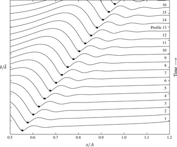
Capillary wave evolution following early events in figure 6. The timespan is
 $t^{\ast }=\tilde{t}/{\it\tau}\in [3.95:0.2:7.15]$
(time scale
 ${\it\tau}$
as in figure 6). Growth of the first capillary trough kicks off the creation of additional capillary humps/troughs of decreasing curvature magnitude.

Emergence of a capillary trough at the foot of the main wave front thus requires that the locus of the free-surface curvature maximum separates from that of the global wave trough. These loci coincide for the harmonic perturbation to which the film is initially subjected, and their separation is caused by the non-symmetric growth of the main hump. This ingredient is already contained in the kinematic waves plotted in figure 2, where open circles mark the curvature maximum and filled circles the film-thickness minimum.
A consequence of the growing capillary wave trough in figure 6 is that it produces a local maximum of negative curvature slightly further downstream (figure 7), owing to the necessity to ‘reconnect’ the free surface to the predominantly flat film separating neighbouring large wave humps. This negative curvature generates the capillary hump seen to emerge from the tenth profile onwards in figure 6. Figure 7(b), where the locus of the capillary hump is highlighted with a diamond, suggests that this is again caused by the curvature-related inertial growth mechanism. Because this mechanism is self-amplifying, the capillary hump, just as the capillary trough, quickly grows as time progresses (figure 6). Figure 8 shows this evolution at later times. Therein, we see that growth of the first capillary hump eventually generates a second capillary trough further downstream, which itself produces another capillary hump and so on and so forth. This series of capillary humps, ‘sandwiched’ between capillary troughs, are what we call ‘capillary waves’.
Given that the physical explanations presented above are based on equation (2.2), which, strictly speaking, is not valid for wave regimes deviating substantially from the primary flow, we check them against the Navier–Stokes equations. We will show that the latter confirm the main physical mechanisms identified with (2.2). For this, we focus on two of the profiles in figures 6 and 8: (i) the eighth profile in figure 6 (
 $t^{\ast }=2.15$
) where the capillary trough is just about to appear, and (ii) the thirteenth profile in figure 8 (
 $t^{\ast }=6.55$
) where the capillary waves are much closer to saturation.
To untangle the different mechanisms governing
 $\partial _{t}{\it\delta}$
, we derive a similar expression to (2.2) based on the Navier–Stokes equations. This is done in three steps successively applied to the differential
 $x$
-momentum balance. First, isolate
 $\partial _{yy}u$
(crosswise viscous-diffusion term) and integrate in
 $y$
direction twice to isolate the streamwise velocity
 $u(y)$
(using
 $u|_{y=0}=0$
and
 $\partial _{y}u|_{y={\it\delta}}=0$
in the process). Second, integrate across the film thickness to isolate the flow rate
 $q=\int _{0}^{{\it\delta}}u(y)\,\text{d}y$
:
 $$\begin{eqnarray}\displaystyle q & = & \displaystyle \underbrace{\mathit{Re}\int _{0}^{{\it\delta}}\int _{0}^{y}\int _{y}^{{\it\delta}}-\frac{\text{d}u}{\text{d}t}\,\text{d}^{3}y}_{T_{i}}+\underbrace{\mathit{Re}\int _{0}^{{\it\delta}}\int _{0}^{y}\int _{y}^{{\it\delta}}-\partial _{x}p\,\text{d}^{3}y}_{T_{p}}\nonumber\\ \displaystyle & & \displaystyle +\,\underbrace{3\int _{0}^{{\it\delta}}\int _{0}^{y}\int _{y}^{{\it\delta}}\text{d}^{3}y}_{T_{g}}+\underbrace{\int _{0}^{{\it\delta}}\int _{0}^{y}\int _{y}^{{\it\delta}}\partial _{xx}u\,\text{d}^{3}y}_{T_{{\it\mu}}}.\end{eqnarray}$$
Third, differentiate in the streamwise direction to isolate
 $\partial _{t}{\it\delta}=-\partial _{x}q$
:
 $$\begin{eqnarray}\partial _{t}{\it\delta}=-\partial _{x}q=-\partial _{x}T_{i}-\partial _{x}T_{p}-\partial _{x}T_{g}-\partial _{x}T_{{\it\mu}}.\end{eqnarray}$$
This equation can be applied to the DNS data to quantify the growth-rate contributions of inertia, pressure, gravity and streamwise viscous diffusion (
 $T_{i}$
,
 $T_{p}$
,
 $T_{g}$
, and
 $T_{{\it\mu}}$
). Figure 9 represents profiles of the dominant terms in (3.2b
) (figure 9
b,d) as well as the corresponding free-surface profiles (figure 9
a,c) at the two above-mentioned time points. Plus signs mark the locus of the main wave maximum, open circles that of the curvature maximum (roughly where the first capillary trough appears), and filled circles that of the adjacent local-curvature minimum (roughly where the first capillary hump appears). Dashed lines in figure 9(b,d) represent the growth rate
 $\partial _{t}{\it\delta}$
. The contribution of gravity, just as for kinematic waves (2.7), can be evaluated to
 $-\partial _{x}T_{g}=-3\partial _{x}{\it\delta}$
and is plotted with dot-dashed lines. It is null at extrema and cannot explain the growth nor decay of capillary humps and troughs. Rather, this growth is governed by a balance between the destabilizing effect of inertia
 $-\partial _{x}T_{i}$
and the stabilizing effects of capillary-induced pressure gradients
 $-\partial _{x}T_{p}$
and streamwise viscous diffusion
 $-\partial _{x}T_{{\it\mu}}$
. Solid lines in figure 9(b,d) represent this balance, i.e.
 $-\partial _{x}(T_{i}+T_{p}+T_{{\it\mu}})$
.
Different contributions to the growth rate
 $\partial _{t}{\it\delta}$
in the region of the capillary waves for two different time points. (a,b) Early stage (eighth profile in figure 6,
 $t^{\ast }=2.15$
); (c,d) wave structure closer to saturation (thirteenth profile in figure 8,
 $t^{\ast }=6.55$
). (a,b) Depict film-thickness profiles, and (c,d) profiles of different contributions to the growth rate according to (3.2b
). Dashed lines:
 $\partial _{t}{\it\delta}$
; dot-dashed lines:
 $-\partial _{x}T_{g}=-3\partial _{x}{\it\delta}$
; solid lines:
 $-\partial _{x}(T_{i}+T_{p}+T_{{\it\mu}})$
; open circles: curvature maximum; filled circles: local curvature minimum.

Starting with the earlier time point (figure 9
a,b), we see that the kinematic growth-rate contribution (dot-dashed line in figure 9
b) follows the gradient of the wave profile, assuming negative values in the wave back, positive values in the wave front and zero at the extrema. The growth rate
 $\partial _{t}{\it\delta}$
(dashed line) roughly follows this evolution with two exceptions:
 $\partial _{t}{\it\delta}$
is positive at the main wave hump (plus sign), which is thus growing, and negative at the position where the first capillary trough is about to appear (slightly downstream of the open circle). Inspecting the profile of
 $-\partial _{x}(T_{i}+T_{p}+T_{{\it\mu}})$
(solid line in figure 9
b), which is positive at the first and negative at the second position, we deduce that this growth follows from an excess in the destabilizing inertial contribution
 $-\partial _{x}T_{i}$
. Our qualitative statements based on (2.2) are thus confirmed.
As the capillary waves approach saturation, we expect the stabilizing growth-rate contributions
 $-\partial _{x}T_{p}$
and
 $-\partial _{x}T_{{\it\mu}}$
to play an increasing role. This is confirmed by figure 9(c,d). Therein, we observe that
 $-\partial _{x}T_{p}$
and
 $-\partial _{x}T_{{\it\mu}}$
have taken the upper hand at both the capillary trough (open circle) and hump (filled circle), causing a slight reversal of growth rates there. Incidentally, these stabilizing contributions already play a role at the earlier time point (figure 9
b) as they significantly counteract the inertial effect at the curvature maximum (open circle), which contributes to moving the point where the first capillary trough will appear slightly downstream.
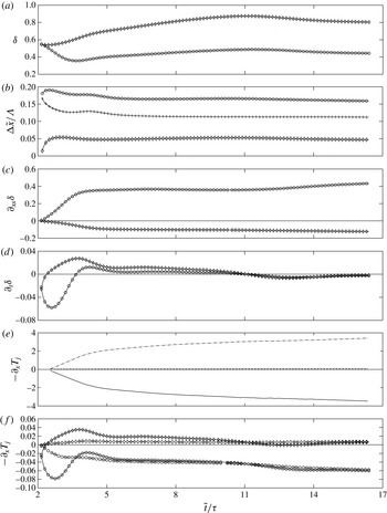
Figure 10 shows the time evolution of the mechanisms at play during inception, growth and attenuation of the first capillary trough and hump. It represents time traces of the film thickness (figure 10
a), free-surface curvature (figure 10
c) and growth rate
 $\partial _{t}{\it\delta}$
(figure 10
d), as well as individual contributions
 $-\partial _{x}T_{i}$
,
 $-\partial _{x}T_{p}$
, and
 $+\partial _{x}T_{{\it\mu}}$
(figure 10
e,f). Thereby,
 $T_{{\it\mu}}$
was approximated with
 $\partial _{xx}(q/{\it\delta}){\it\delta}^{3}/3$
to avoid excessive error amplification when differentiating the numerical data. In addition, figure 10(b) depicts time traces of the streamwise separation
 ${\rm\Delta}x$
between main-hump/capillary-trough (plus signs), capillary-trough/capillary-hump (diamonds) and main-hump/capillary-hump (circles).
Figure 10(a) shows that the capillary trough (circles) increasingly deepens in the early stages, reaches a minimum, and then slowly approaches its saturated depth. The corresponding free-surface curvature (figure 10
c) is correlated quite well with the depth of the trough but it is also affected by its width (figure 10
b). Reciprocal observations apply to the first capillary hump (diamonds). In terms of the mechanisms underlying these kinematics, figure 10(e) confirms our prior assumption that the growth-rate contribution of inertia
 $-\partial _{x}T_{i}$
(solid line) is destabilizing, while those of pressure
 $-\partial _{x}T_{p}$
(dot-dashed line) and streamwise viscous diffusion
 $-\partial _{x}T_{{\it\mu}}$
(dashed line) are stabilizing. Indeed, at the capillary trough,
 $-\partial _{x}T_{i}$
is negative while the other terms are positive (the opposite applies to the capillary hump, which is not shown here). We point out that
 $-\partial _{x}T_{i}$
and
 $-\partial _{x}T_{p}$
in the earliest stages are exceedingly small and could not be (individually) evaluated reliably due to numerical errors. These data were omitted from figure 10(e).
Of course, the growth rate
 $\partial _{t}{\it\delta}$
is finally determined by a balance of the three effects. Although the inertial and pressure terms are far greater in magnitude than the viscous term, the latter still plays an important role as the former partially cancel each other. This is shown in figure 10(f), which compares
 $-\partial _{x}T_{i}-\partial _{x}T_{p}$
to
 $+\partial _{x}T_{{\it\mu}}$
at the capillary trough (circles) and hump (diamonds), respectively (note that
 $+\partial _{x}T_{{\it\mu}}$
and not
 $-\partial _{x}T_{{\it\mu}}$
is plotted here to better compare magnitudes of same-symbol curves). We see that
 $-\partial _{x}T_{i}-\partial _{x}T_{p}$
and
 $-\partial _{x}T_{{\it\mu}}$
are comparable in magnitude, meaning that streamwise viscous diffusion significantly shapes capillary waves in falling liquid films. This is in line with Ruyer-Quil & Manneville (Reference Ruyer-Quil and Manneville2000), who showed that taking it into account in their model significantly damped the capillary waves (see figure 5 in that reference). The destabilizing effect of inertia
 $-\partial _{x}T_{i}$
by and large surmounts the stabilizing effect of pressure
 $-\partial _{x}T_{p}$
, meaning that variations of
 $-\partial _{x}T_{i}-\partial _{x}T_{p}$
in magnitude (as compared to
 $-\partial _{x}T_{{\it\mu}}$
) and not in sign dictate whether the capillary waves grow or decay. This is confirmed by the strong correlation between
 $\partial _{t}{\it\delta}$
(figure 10
d) and
 $|-\partial _{x}T_{i}-\partial _{x}T_{p}|$
(figure 10
f).
Dynamics of capillary ripples. Time traces at the first capillary trough (circles) and hump (diamonds). (a,c,d) Film thickness, free-surface curvature and growth rate; (b) distance between main-hump/capillary-trough (plus signs), capillary-trough/capillary-hump (diamonds), and capillary-hump/main-hump (circles); (e) different growth-rate contributions at the first capillary trough according to (3.2b
): inertia
 $-\partial _{x}T_{i}$
(solid line), pressure
 $-\partial _{x}T_{p}$
(dot-dashed line) and streamwise viscous diffusion
 $-\partial _{x}T_{{\it\mu}}$
(dashed line); (f) comparison of
 $-\partial _{x}T_{i}-\partial _{x}T_{p}$
(solid line) and
 $+\partial _{x}T_{{\it\mu}}$
(dashed line). Inertia drives growth of the capillary trough and hump against the stabilizing effects of capillary-induced pressure gradients and streamwise viscous diffusion.

By comparing the mechanical contributions plotted in figure 10(e,f) with the kinematic quantities plotted in figure 10(a–d), we may draw the following main conclusions. Inertia is indeed responsible for the inception and growth of the first capillary trough. This growth is arrested by capillary-induced pressure gradients and streamwise viscous diffusion once the local film thickness (figure 10 a) and the width of the capillary trough (figure 10 b) have become sufficiently small, while the local curvature (figure 10 c) has become large. Indeed, increasingly compressing the deepening capillary trough between the main and capillary humps creates large gradients of curvature (augmenting capillary-induced pressure gradients) and film thickness (augmenting streamwise velocity gradients and viscous stresses). Reciprocal observations apply to the first capillary hump, which saturates at a much smaller amplitude than the main hump because the short wavelength imposed by the capillary trough immediately produces large curvature gradients. The smaller capillary hump in turn produces a less pronounced second capillary trough and so on and so forth. Precursory capillary ripples, which are initiated in the most curved portion of the steepening front of a single-peaked wave hump, thus come to their saturation in the form of a compressed (and attenuating) capillary wave train, exhibiting large gradients in free-surface curvature and film thickness.
4. Celerity matching: how do capillary waves keep up?
In this section, we investigate through what mechanism capillary waves eventually adjust their celerity to that of the much greater main humps. Evaluating
 $c=\partial _{x}q/\partial _{x}{\it\delta}$
at extremal points using l’Hôpital’s rule (
 $\partial _{x}{\it\delta}=0$
and, if
 $c$
is assumed to be finite,
 $\partial _{x}q$
must also tend to zero), yields the celerity
 $c|_{x=x_{E}}=\partial _{xx}q/\partial _{xx}{\it\delta}|_{x=x_{E}}$
there, which may be decomposed into its respective dynamic contributions based on (3.2a
):
 $$\begin{eqnarray}c=\frac{\partial _{xx}q}{\partial _{xx}{\it\delta}}=\underbrace{\partial _{xx}T_{i}/\partial _{xx}{\it\delta}}_{c_{i}}+\underbrace{\partial _{xx}T_{p}/\partial _{xx}{\it\delta}}_{c_{p}}+\underbrace{\partial _{xx}T_{g}/\partial _{xx}{\it\delta}}_{c_{g}}+\underbrace{\partial _{xx}T_{{\it\mu}}/\partial _{xx}{\it\delta}}_{c_{{\it\mu}}},\end{eqnarray}$$
where the subscript
 $x=x_{E}$
was omitted for convenience. The contribution of gravity can be evaluated to
 $c_{g}=3{\it\delta}^{2}$
and corresponds to the celerity of kinematic waves (2.7). Strictly speaking, (4.1) only holds for waves of constant amplitude, i.e. when
 $\text{d}{\it\delta}=0$
, but we will nonetheless apply it to characterize conditions prior to saturation. This amounts to a quasi-stationary treatment of the celerity evolution.
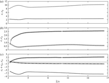
Time evolution (
 ${\it\tau}$
as in figure 8) of different contributions to the wave celerity according to (4.1) evaluated at the main hump (plus signs) and capillary trough (open circles). (a,b) Full celerity
 $c$
(solid lines) and contribution of gravity
 $c_{g}$
(symbols only); (c) resulting contribution of inertia and pressure
 $c_{i}+c_{p}$
(solid line) and contribution of streamwise viscous diffusion
 $c_{{\it\mu}}$
(dashed line). At the hump,
 $c_{{\it\mu}}$
is noisy but negligibly small and thus not shown.

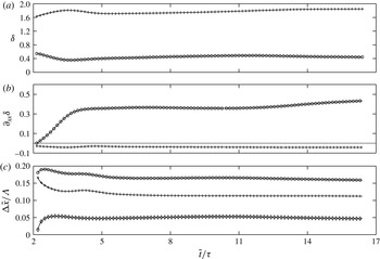
Evolution (
 ${\it\tau}$
as in figure 8) of the shape of the main hump (plus signs) and capillary trough (open circles) over the time span in figure 11. (a) Film thickness
 ${\it\delta}$
; (b) free-surface curvature
 $\partial _{xx}{\it\delta}$
; (c) streamwise separation between main-hump/capillary-hump (open circles), main-hump/capillary-trough (plus signs) and capillary-trough/capillary-hump (diamonds).

The different celerity contributions in (4.1) are plotted in figure 11 (over the same timespan as figure 10) at the main hump (plus signs) and capillary trough (open circles), respectively, while figure 12 plots the corresponding film thickness, curvature and streamwise separation. Figure 11(a,b) show that the kinematic contribution
 $c_{g}$
(symbol-only curves) tends to impose a much greater celerity at the main hump than at the capillary trough, owing to the considerable difference in film thickness between these locations. Nonetheless, the full celerity
 $c$
(solid lines) at the two extrema is eventually matched at
 $c\approx 2.5$
. In the process, the celerity of the main hump drops much more significantly with respect to
 $c_{g}$
than that of the capillary trough rises. This is driven by the interplay between the contributions of capillary-induced pressure variations
 $c_{p}$
and inertia
 $c_{i}$
.
Separate evaluation of these contributions proved problematic due to amplification of numerical errors that withstood the good spatio-temporal resolution of our simulation (the time increment was
 ${\rm\Delta}\tilde{t}=10^{-8}$
s and the minimal film thickness
 $\tilde{{\it\delta}}_{\text{min}}\approx 150\,{\rm\mu}\text{m}$
was resolved with about 25 grid points). However, for the larger
 $\mathit{Re}$
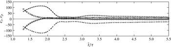
simulation in figure 20, the problem is lesser. We thus refer to figure 21 in appendix A, which plots separate time traces of
 $c_{p}$
and
 $c_{i}$
for that very similar simulation. These show that the celerity of the capillary trough is increased by capillary-induced pressure gradients (
 $c_{p}>0$
, dot-dashed lines) and decreased by inertia (
 $c_{i}<0$
, solid lines), while the opposite holds at the main hump (
 $c_{p}<0,\,c_{i}>0$
). The sum of the two celerity contributions
 $c_{i}+c_{p}$
is plotted in figure 11(c) (solid lines), showing that
 $c_{p}$
dominates
 $c_{i}$
, which increases the celerity of the capillary trough and decreases that of the main hump. Meanwhile, the contribution of streamwise viscous diffusion
 $c_{{\it\mu}}$
is considerable at the capillary trough (dashed line), decreasing its speed, and negligibly small at the hump (data not plotted).
Comparing solid lines in figure 11(a,b), we see that the capillary trough initially travels much (two times) slower than the main hump and then speeds up significantly, while the main hump slows down only slightly. The acceleration of the capillary trough is driven by the streamwise separation between main hump and capillary trough/hump. Indeed, in the early stages, the fast-approaching main hump increasingly compresses the capillary trough (figure 12
c), while increasing its curvature (figure 12
b). This in turn causes
 $|c_{p}|$
to rise with respect to
 $|c_{i}|$
(figure 11
c) and thus speeds up the capillary trough. We point out that similar mechanics govern the evolution of all subsequent capillary humps and troughs, until all celerities are matched and all amplitudes are saturated.
The main hump’s celerity (figure 11
a) and amplitude (figure 12
a) are arrested when the leading wave front steepens (figure 12
c) while coming up on the initially slow capillary trough, increasing
 $|\partial _{xx}{\it\delta}|$
at the wave maximum (figure 12
b). In this sense, we may also conclude that capillary waves limit the celerity and amplitude of the main humps.
In summary, celerity matching between main humps and capillary waves is achieved when these structures are compressed into a wave train of sufficiently large free-surface curvature magnitudes at the extrema, allowing capillary-induced pressure gradients
 $c_{p}$
(and streamwise viscous diffusion
 $c_{{\it\mu}}$
) to slow down the main hump and speed up the capillary trough. We observed in § 2 that these mechanisms strongly scale with
 ${\it\delta}$
. Assuming this holds qualitatively in figure 12, it explains why
 $|\partial _{xx}{\it\delta}|$
at the capillary trough is much greater than at the main hump (figure 12
c).
Wavenumber of first capillary wave
 ${\it\alpha}_{c}=2{\rm\pi}\tilde{{\it\delta}}_{0}/{\it\Lambda}_{c}$
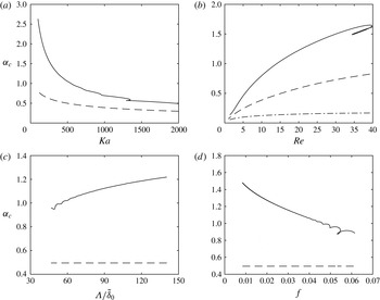
(solid lines) compared to visco-capillary cutoff of the Kapitza instability (dashed lines). Solid lines: simplified second-order WRIBL model (Ruyer-Quil & Manneville Reference Ruyer-Quil and Manneville2000); dashed lines: Orr–Sommerfeld temporal linear stability analysis (Brooke Benjamin Reference Brooke Benjamin1957). Parameters vary about case 1 in table 1: (a) influence of the Kapitza number
 $Ka={\it\sigma}/({\it\rho}\,g^{1/3}\,{\it\nu}^{4/3})$
; (b) influence of the Reynolds number
 $\mathit{Re}$
; (c) influence of the large hump wavelength
 ${\it\Lambda}$
; (d) influence of the large hump frequency
 $f$
. All quantities are non-dimensionalized with primary flow scales except for the dot-dashed line in (b) which rescales the dashed-line data using
 $\tilde{{\it\delta}}_{{\it\nu}}=({\it\mu}/{\it\rho})^{2/3}g^{-1/3}=93.9~{\rm\mu}$
m. The wave number of capillary waves is systematically greater than the visco-capillary cutoff. Thus, these waves are stable in terms of the primary Kapitza instability and justly designated as ‘capillary waves’.

5. Why are they called ‘capillary waves’?
Throughout this manuscript, we have used the words ‘capillary waves’ to designate the small ripples preceding the large wave humps in figure 1. However, we have not explained the capillary nature of these ripples. We have shown that their growth is arrested by surface tension forces (as well as streamwise viscous diffusion), but this is also true for the main wave humps. Something else must thus be at play.
It turns out that the wavelength of capillary waves on falling liquid films is systematically shorter than the visco-capillary cutoff wavelength of the Kapitza instability. Figure 13 shows this for a large variety of wave trains (see figures 17–19 for profiles) computed using the simplified second-order WRIBL model of Ruyer-Quil & Manneville (Reference Ruyer-Quil and Manneville2000), which has been validated against experiments and DNS in appendix A. This model, coupled with the continuation software Auto07P (Doedel Reference Doedel2007), allowed parameter sweeps at moderate computational cost. Solid lines in figure 13(a–d) represent the dimensionless wavenumber of the first capillary wave
 ${\it\alpha}_{c}=2{\rm\pi}\tilde{{\it\delta}}_{0}/{\it\Lambda}_{c}$
, where
 ${\it\Lambda}_{c}$
is the streamwise distance between the first and second capillary trough, as a function of the Kapitza number
 $Ka$
, Reynolds number
 $\mathit{Re}$
, wavelength
 ${\it\Lambda}$
and frequency
 $f$
, respectively. We use the Kapitza number
 $Ka={\it\sigma}/({\it\rho}\,g^{1/3}\,{\it\nu}^{4/3})$
here instead of the Bond number because it contains only fluid properties.
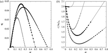
Temporal linear stability data obtained from Orr–Sommerfeld solution. (a) Growth rate
 ${\it\Psi}$
(non-dimensionalized with
 $\tilde{{\it\delta}}_{0}/\tilde{u} _{0}|_{\tilde{{\it\delta}}_{0}}$
) versus wave number; (b) celerity versus wavenumber. Parameters vary about case 1 (filled circles) in table 1. ●:
 $\mathit{Re}=15$
,
 $Ka=509.5$
; ▾:
 $\mathit{Re}=1$
,
 $Ka=509.5$
; ♦:
 $\mathit{Re}=30$
,
 $Ka=509.5$
;
 $+$
:
 $\mathit{Re}=15$
,
 $Ka=2000$
. The visco-capillary cutoff wavenumber (a) decreases with decreasing Reynolds number and increasing Kapitza number. Celerity-matched waves of increasingly disparate wave number are possible beyond the unstable branch (highlighted by symbols in (b)), especially at large
 $\mathit{Re}$
and low
 $Ka$
.

Dashed lines in figure 13(a–d) represent the visco-capillary cutoff wavenumber of the primary Kapitza instability, which was obtained by linear stability analysis of the Navier–Stokes equations (Brooke Benjamin Reference Brooke Benjamin1957; Yih Reference Yih1963). It is apparent in figure 14(a), plotting linear temporal growth rate versus wavenumber for selected parameter combinations. The cutoff wavenumber is the short-wave intersection with the
 ${\it\alpha}$
-axis and decreases with decreasing Reynolds number/increasing Kapitza number. It is of visco-capillary nature because both surface tension and streamwise viscous diffusion (see figure 3 in Ruyer-Quil & Manneville (Reference Ruyer-Quil and Manneville1998)) stabilize the inertia-driven Kapitza instability.
Comparing solid and dashed lines in figure 13, we may thus conclude: capillary waves on falling liquid films are systematically shorter than the visco-capillary cutoff wavelength of the Kapitza instability, are thus dominated by (visco–)capillary forces, and justly designated as ‘capillary waves’. Regarding the earlier cited statements of Chang (Reference Chang1994), we may observe that, although the trend of the capillary wavenumber in terms of the control parameters (except for frequency) is roughly in agreement with that of the linear cutoff wavenumber, there is a significant disagreement between the actual values.
Comparing the wavenumber of the nonlinear capillary waves with the linear cutoff wavenumber for the primary flow is not precisely adequate because the local Reynolds number in the capillary wave region is smaller. However, taking into account a lower Reynolds number, would yield an even lower linear cutoff wavenumber (dot-dashed line in figure 13 b). Meanwhile, the ‘wiggles’ of the solid curves in figure 13(c,d) appear at small wavelengths and large frequencies when the capillary waves directly interact with the back of the next main hump. Each ‘wiggle’ is associated with the addition/subtraction of a capillary hump to/from the train of capillary waves.
We add an observation regarding the linear celerity curves plotted in figure 14(b). These curves are composed of a branch that decreases and one that increases with wavenumber. Thus, the linear behaviour of falling liquid films already allows waves of different wavelength to be matched in celerity. To accommodate considerably disparate wavelengths, the short waves (large wavenumber) must exit the unstable part of the celerity curve (highlighted by symbols), i.e. transcend the visco-capillary cutoff.
The above conclusions imply that capillary waves on falling liquid films are linearly stable in terms of the Kapitza instability and should attenuate if they were travelling on their own. How is it then possible that they nonetheless attain/maintain a finite amplitude? This could not work if they would behave like capillary waves in the sense of Whitham (Reference Whitham1974), the celerity of which depends only on their wavenumber:
 $$\begin{eqnarray}\tilde{c}=[({\it\sigma}\,\tilde{{\it\alpha}}/{\it\rho})\tanh (\tilde{{\it\alpha}}\,\tilde{{\it\delta}})]^{1/2}.\end{eqnarray}$$
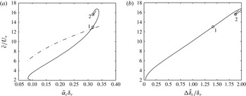
Figure 15(a) compares this relation (dot-dashed line) with the celerity of the nonlinear capillary waves (solid line), showing a clear discrepancy. Indeed, the nonlinear celerity curve shows that capillary waves of the same wavenumber may travel at different celerities (e.g. points 1 and 2), which is not compatible with (5.1). This is because their celerity also depends on their amplitude, as shown in figure 15(b). More specifically, the capillary wave celerity increases with amplitude. Consequently, considering a capillary wave travelling in front of a main wave hump, it will tend to attenuate due to its linear stability, but this would reduce its celerity, causing the main hump to catch up and compress/speed-up the capillary wave once again (§ 4). We can thus conclude that large wave humps travelling on falling liquid films continuously transfer energy to the precursory capillary ripples for these to maintain a finite amplitude. This is comparable to capillary wakes of objects travelling on liquid surfaces (Raphaël & de Gennes Reference Raphaël and de Gennes1996; Moisy & Rabaud Reference Moisy and Rabaud2014).
Celerity of capillary waves. (a) Influence of the wavenumber. Solid line: nonlinear waves from figure 13(a); dot-dashed line: conventional capillary waves in the sense of Whitham (Reference Whitham1974)
 $\tilde{c}=[({\it\sigma}\,\tilde{{\it\alpha}}/{\it\rho})\tanh (\tilde{{\it\alpha}}\,\tilde{{\it\delta}})]^{1/2}$
; (b) influence of the wave amplitude (nonlinear waves), i.e. the height difference between first capillary trough and hump
 ${\rm\Delta}\tilde{{\it\delta}}$
. Here, natural scales are used for non-dimensionalization:
 ${\it\delta}_{{\it\nu}}=({\it\mu}/{\it\rho})^{2/3}g^{-1/3}$
and
 $U_{{\it\nu}}=({\it\mu}\,g/{\it\rho})^{1/3}$
. Contrary to conventional capillary waves, the celerity of capillary waves on falling liquid films depends on their amplitude.

6. Capillary waves in fully-developed wave trains
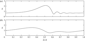
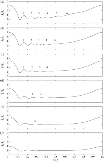
Once the mechanisms governing the amplitude and celerity of main humps and capillary ripples have settled into an equilibrium, the final wave shape in figure 16 is obtained. Figure 16(a) represents case 1 and figure 16(b) case 2, which has a different Reynolds number and wavelength (see table 1). Comparing the two panels, we see that the capillary ripples are significantly altered by changing the wavelength and amplitude of the main humps. We proceed by explaining how this relation is natured based on physical insights from the previous sections. To do so, we again consider the parameter variations performed for figure 13 using the WRIBL model of Ruyer-Quil & Manneville (Reference Ruyer-Quil and Manneville2000).
We start by varying the Reynolds number
 $\mathit{Re}$
around the WRIBL simulation of case 1, while maintaining the Kapitza number and wavelength constant. Figure 17 shows wave profiles obtained this way, with
 $\mathit{Re}$
decreasing from (a) to (f). The amplitude of the main humps increases with the Reynolds number due to the mounting relevance of inertia (
 $T_{i}$
in (3.2)) and also increases their celerity. This compresses the precursory capillary waves more and more into a train of increasing curvatures
 $|\partial _{xx}{\it\delta}|$
and decreasing wavelength, so that capillary and viscous effects (
 $T_{p}$
,
 $T_{{\it\mu}}$
and
 $c_{p}$
,
 $c_{{\it\mu}}$
in (3.2) and (4.1)) may arrest the rising inertial contributions and produce a saturated and phase-locked solution. Meanwhile, the number of precursory capillary waves rises with increasing
 $\mathit{Re}$
, which results from the increasing curvature
 $\partial _{xx}{\it\delta}$
of the first capillary trough. Indeed, the number of capillary waves is fixed by the condition that the last of the spatially-attenuating capillary troughs must transition smoothly to the back of the next main hump. Consequently, when the curvature of the first capillary trough is greater, additional spatially-attenuating ripples are needed to sufficiently reduce
 $\partial _{xx}{\it\delta}$
.
Saturated shape of a train of solitary pulses on a falling liquid film, consisting of a main hump and precursory capillary waves, obtained from DNS for cases 1 and 2 in table 1. (a) Case 1:
 $\mathit{Re}=15$
,
 $f=16$
Hz; (b) case 2:
 $\mathit{Re}=10.7$
,
 $f=20$
Hz. Capillary waves are strongly modified by changing the wavelength and amplitude of the large wave humps.

Influence of Reynolds number on amplitude, wavelength and number of capillary waves:
 $Ka=509.5$
;
 ${\it\Lambda}/\tilde{{\it\delta}}_{{\it\nu}}=226$
, fluid properties according to table 1. Length scale:
 $\tilde{{\it\delta}}_{{\it\nu}}=({\it\mu}/{\it\rho})^{2/3}g^{-1/3}$
. (a)
 $\mathit{Re}=40$
,
 $\tilde{c}=0.497$
m s
 $^{-1}$
; (b)
 $\mathit{Re}=30$
,
 $\tilde{c}=0.450$
m s
 $^{-1}$
; (c)
 $\mathit{Re}=20$
,
 $\tilde{c}=0.384$
m s
 $^{-1}$
; (d)
 $\mathit{Re}=15$
(case 1, table 1),
 $\tilde{c}=0.342$
m s
 $^{-1}$
; (e)
 $\mathit{Re}=10$
,
 $\tilde{c}=0.288$
m s
 $^{-1}$
; (f)
 $\mathit{Re}=5$
,
 $\tilde{c}=0.202$
m s
 $^{-1}$
. Simulations with simplified second-order WRIBL model (Ruyer-Quil & Manneville Reference Ruyer-Quil and Manneville2000). Increasing
 $\mathit{Re}$
increases amplitude of main humps, increasingly compressing capillary waves.

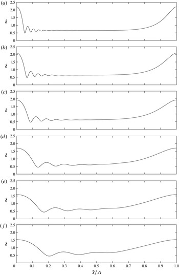
Influence of large hump wavelength
 ${\it\Lambda}$
on amplitude, wavelength and number of capillary waves:
 $Ka=509.5$
;
 $\mathit{Re}=15$
, fluid properties according to table 1. (a)
 ${\it\Lambda}/\tilde{{\it\delta}}_{0}=140$
,
 $\tilde{c}=0.438$
m s
 $^{-1}$
; (b)
 ${\it\Lambda}/\tilde{{\it\delta}}_{0}=112$
,
 $\tilde{c}=0.410$
m s
 $^{-1}$
; (c)
 ${\it\Lambda}/{\it\delta}_{0}=84$
,
 $\tilde{c}=0.375$
m s
 $^{-1}$
; (d)
 ${\it\Lambda}/\tilde{{\it\delta}}_{0}=56$
,
 $\tilde{c}=0.330$
m s
 $^{-1}$
; (e)
 ${\it\Lambda}/\tilde{{\it\delta}}_{0}=45$
,
 $\tilde{c}=0.308$
m s
 $^{-1}$
; (f)
 ${\it\Lambda}/\tilde{{\it\delta}}_{0}=38$
,
 $\tilde{c}=0.293$
m s
 $^{-1}$
. Simulations with simplified second-order WRIBL model (Ruyer-Quil & Manneville Reference Ruyer-Quil and Manneville2000). Increasing
 ${\it\Lambda}$
increases the amplitude of main humps, increasingly compressing capillary waves.

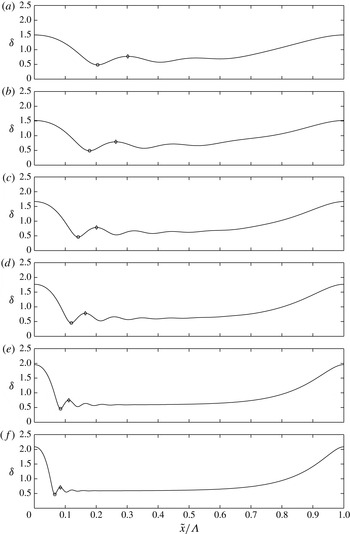
Influence of Kapitza number
 $Ka={\it\sigma}/({\it\rho}\,g^{1/3}\,{\it\nu}^{4/3})$
on amplitude, wavelength and number of capillary waves:
 $\mathit{Re}=15$
;
 ${\it\Lambda}/\tilde{{\it\delta}}_{0}=63.4$
, fluid properties (except
 ${\it\sigma}$
) according to table 1. (a)
 $Ka=2000$
,
 $\tilde{c}=0.322$
m s
 $^{-1}$
; (b)
 $Ka=1400$
,
 $\tilde{c}=0.318$
m s
 $^{-1}$
; (c)
 $Ka=800$
,
 $\tilde{c}=0.333$
m s
 $^{-1}$
; (d)
 $Ka=510$
(case 1, table 1),
 $\tilde{c}=0.343$
m s
 $^{-1}$
; (e)
 $Ka=200$
,
 $\tilde{c}=0.358$
m s
 $^{-1}$
; (f)
 $Ka=100$
,
 $\tilde{c}=0.366$
m s
 $^{-1}$
. Simulations with simplified second-order WRIBL model (Ruyer-Quil & Manneville Reference Ruyer-Quil and Manneville2000). Decreasing
 $Ka$
increases curvature
 $\partial _{xx}{\it\delta}|_{\circ }$
by compression of the capillary wave train, until streamwise viscous diffusion becomes strong and dampens the capillary amplitude.
 $\partial _{t}{\it\delta}_{{\it\mu}}|_{\circ }=-0.68$
(a),
 $-$
0.95 (b),
 $-$
2.16 (c),
 $-$
3.65 (d),
 $-$
8.91 (e),
 $-$
15.19 (f);
 $\partial _{t}{\it\delta}_{p}|_{\circ }=-2.73$
(a),
 $-$
2.95 (b),
 $-$
4.83 (c),
 $-$
6.88 (d),
 $-$
13.19 (e),
 $-$
20.63 (f);
 $(\partial _{t}{\it\delta}_{{\it\mu}}/\partial _{t}{\it\delta}_{p})|_{\circ }=0.25$
(a), 0.32 (b), 0.45 (c), 0.53 (d), 0.68 (e), 0.74 (f);
 $\partial _{xx}|_{\circ }=0.067$
(a), 0.093 (b), 0.210 (c), 0.359 (d), 0.928 (e), 1.667 (f);
 ${\it\delta}_{\diamond }-{\it\delta}|_{\circ }=0.29$
(a), 0.30 (b), 0.32 (c), 0.33 (d), 0.29 (e), 0.23 (f).

Figure 18 shows the effect of the large-hump wavelength
 ${\it\Lambda}$
. Increasing
 ${\it\Lambda}$
(from (f) to (a)) while maintaining the Reynolds and Kapitza numbers constant, increases the linear growth rate of the primary Kapitza instability and, consequently, the amplitude of the large humps. Similarly to the previous figure, this creates increasingly compressed capillary waves of rising number. In contrast to figure 17, the three cases with largest amplitude (figure 18
a–c) develop a flat residual film. This results from the way in which the increase in height of the main humps is sustained in figures 18 and 17, respectively. In figure 18, the Reynolds number and thus the mean film thickness are constant so that the region between two subsequent main humps must increasingly drain in order to sustain their growth. Conversely, in figure 17, the increase in wave height is in part sustained by increasing the mean film thickness, which increases with
 $\mathit{Re}$
.
Once this flat residual film has formed, the last capillary hump/trough can always smoothly connect to it (as
 $\partial _{x}{\it\delta}=0$
there) and so the number of capillary ripples ceases to increase. Instead, the length of the capillary wave train is simply shortened. Incidentally, transition from capillary waves interacting with the back of the next main hump to formation of a flat residual film coincides with the ‘wiggles’ in figure 13(c,d).
Figure 19 shows the effect of reducing the Kapitza number
 $Ka={\it\sigma}/({\it\rho}\,g^{1/3}\,{\it\nu}^{4/3})$
(from (a) to (f)), which can be achieved e.g. by reducing the surface tension. On the one hand, this directly affects the capillary waves, which increase their curvature magnitude (see
 $\partial _{xx}{\it\delta}$
in figure 19) and decrease their wavelength so that capillary-induced growth rate and celerity contributions (
 $T_{p}$
,
 $c_{p}$
in (3.2) and (4.1)) can be maintained in the face of weakening
 ${\it\sigma}$
, in order to counter inertial contributions (
 $T_{i}$
,
 $c_{i}$
in (3.2) and (4.1)). On the other hand, reducing surface tension means that the main humps saturate at a greater amplitude and thus travel faster, compressing the capillary wave train even further. This indirect
 $Ka$
-effect is comparable to figures 17 and 18.
The amplitude of capillary waves in figure 19(a–d) (see
 ${\it\delta}|_{\diamond }-{\it\delta}|_{\circ }$
in lower right-hand corner) varies very little. Their speed-up mechanism in the face of diminishing
 $Ka$
mainly consists in reducing their wavelength, which is a capacity already exhibited by the linear celerity curves of figure 14(b) (therein, capillary waves are situated beyond the symbol-marked unstable branches). Nonetheless, when the capillary wavelength becomes very small (figure 19
e,f), the capillary amplitude starts to decrease noticeably. This is due to streamwise viscous diffusion (
 $T_{{\it\mu}}$
,
 $c_{{\it\mu}}$
in (3.2), (4.1)), which increases its relative importance as
 $Ka$
diminishes and streamwise velocity gradients between capillary troughs and humps become strong. In this low
 $Ka$
limit, the capillary waves still significantly increase their curvature
 $|\partial _{xx}{\it\delta}|$
with decreasing
 $Ka$
but they do this while reducing both their wavelength and their amplitude. This is in agreement with Ruyer-Quil & Manneville (Reference Ruyer-Quil and Manneville2000) (see figure 5 there), who observed that ‘switching on’ streamwise viscous diffusion in their WRIBL model reduces the capillary amplitude and wavelength.
To explain this intricate effect, we extract the growth-rate contribution of streamwise viscous diffusion
 $\partial _{t}{\it\delta}_{{\it\mu}}$
from the WRIBL model, i.e. equation (41) in Ruyer-Quil & Manneville (Reference Ruyer-Quil and Manneville2000). This is possible in the case of travelling waves, where we may employ
 $q=q_{MF}+c{\it\delta}$
to express the flow rate in terms of the film thickness and the moving-frame flow-rate
 $q_{MF}=q_{0}-c\,\bar{{\it\delta}}<0$
:
 $$\begin{eqnarray}\partial _{t}{\it\delta}_{{\it\mu}}=\frac{1}{\mathit{Re}}\left[4\frac{q_{MF}}{c{\it\delta}^{2}}-\frac{1}{2{\it\delta}}\right](\partial _{x}{\it\delta})^{2}-\frac{1}{\mathit{Re}}\left[6\frac{q_{MF}}{c{\it\delta}}+\frac{3}{2}\right]\partial _{xx}{\it\delta},\end{eqnarray}$$
whereas the capillary contribution
 $\partial _{t}{\it\delta}_{p}=-\partial _{x}T_{p}$
is given by:
 $$\begin{eqnarray}\partial _{t}{\it\delta}_{p}=\frac{5}{2\,c}\frac{1}{\mathit{Bo}\,\mathit{Re}}{\it\delta}\partial _{xxx}{\it\delta}.\end{eqnarray}$$
These two quantities as well as
 $\partial _{t}{\it\delta}_{{\it\mu}}/\partial _{t}{\it\delta}_{p}$
are quantified in figure 19(a–f), confirming that the relative importance of
 $\partial _{t}{\it\delta}_{{\it\mu}}$
rises significantly with decreasing
 $Ka$
.
Inspecting (6.1a
), we see that the right-hand side consists of two terms, one that is proportional to
 $(\partial _{x}{\it\delta})^{2}$
and always negative, and another that is proportional to
 $\partial _{xx}{\it\delta}$
. The second term is active at the capillary humps and troughs, while the first is active in the flanks separating these extrema and does not differentiate between ascending (
 $\partial _{x}{\it\delta}>0$
) and descending (
 $\partial _{x}{\it\delta}<0$
) flanks. Both terms react differently to changes in the wavelength of the capillary waves and this explains how the latter are modified between figure 19(e,f). We have established that the capillary wave train needs to be compressed from figure 19(e,f) to compensate for the loss in surface tension. This compression increases the curvature magnitude at the extrema and thus the magnitude of
 $\partial _{t}{\it\delta}_{{\it\mu}}$
there. However, if the compression were realized at constant amplitude, the increase in slope of the capillary flanks would be too great, producing a too negative
 $\partial _{t}{\it\delta}_{{\it\mu}}$
there. Consequently, this slope is reduced by decreasing the height difference between capillary humps and troughs.
In summary, when streamwise viscous diffusion becomes a coequal stabilizing mechanism (at low
 $Ka$
), capillary waves are, as usual, compressed, producing large curvature magnitudes at the capillary extrema. But, this compression is done at diminishing amplitude in order to reduce the slope of the capillary flanks compared to a constant-amplitude compression. Decreasing the Kapitza number beyond its value in figure 19(f), further reduces the capillary wave amplitude, yet an increasingly curved capillary trough always remains, until the limiting case of a shock (where
 $\partial _{xx}{\it\delta}$
is infinite) is reached at
 ${\it\sigma}=0$
.
7. Conclusion
The typical shape of a fully-developed train of solitary pulses travelling on a vertically falling liquid film is represented in figures 1 and 16. It consists of a large-amplitude asymmetrical (tear-shaped) main hump of long wavelength, which is preceded by a number of small-amplitude small-wavelength ripples, travelling in phase lock. We have investigated these precursory ripples based on direct numerical simulations (§§ 3–5) as well as low-dimensional models (§§ 2 and 6) in order to answer the following questions.
(i) How do precursory ripples form on wavy falling liquid films? Precursory ripples evolve from single-peaked wave solutions once the amplitude of the main hump becomes large and its leading front sufficiently steepens. The first ripple trough does not emerge from the global trough of the single-peaked wave but forms within the leading wave front (figure 6), close to the locus where the free-surface curvature is positively maximal (figure 7). There, the inertia-induced growth-rate contribution (
 $-\partial _{x}T_{i}$
in (3.2b
) and figure 10
f) is dominantly negative, causing a new global trough to form. Thereby, occurrence of a curvature maximum within the leading wave front is a property already exhibited by kinematic waves (figure 2). Growth of the first ripple trough (figure 6) produces a local negative curvature maximum slightly downstream (figure 7), which generates a corresponding ripple-hump and so on and so forth (figure 8) until a train of ripples covers the residual film separating subsequent large humps (figure 16).
(ii) How can capillary waves travel at the same celerity as the main humps? Linear stability analysis (figure 14
b) already shows that waves of disparate wavelengths can travel at the same speed on falling liquid films. Physically, it is the effect of surface-tension forces (as well as streamwise viscous diffusion) that allows large humps and precursory ripples to match their respective celerities. The capillary-induced contribution to the nonlinear wave celerity (
 $c_{p}$
in (4.1) and figure 21) is negative at the main hump, thus slowing it down, and positive at the ripple trough, thus speeding it up. The magnitude of this term in relation to the opposite-sign inertial contribution (
 $c_{i}$
in (4.1) and figure 21) rises when the main hump and ripple trough are increasingly compressed (figures 11 and 12), as the initially fast-travelling main wave catches up with the initially slow-travelling precursory ripple, until phase lock is eventually achieved.
(iii) Why are the precursory ripples designated as ‘capillary waves’? Precursory ripples are justly designated as ‘capillary waves’, because their wavelength is systematically shorter than the visco-capillary cutoff wavelength of the Kapitza instability (figure 13). They are thus stable and would attenuate if they were travelling on their own. That they nonetheless reach a finite amplitude results from a nonlinear effect, namely that their celerity decreases with amplitude (figure 15 b). This tends to slow down decaying capillary waves relative to the pursuing main hump and causes the latter to reapproach and recompress the capillary waves into a faster-travelling shape (see (ii) above). Capillary waves are thus sustained at finite amplitude by the main hump, which constantly transfers energy to compensate dissipation. This is similar to capillary wakes around objects travelling on a liquid surface (Raphaël & de Gennes Reference Raphaël and de Gennes1996; Moisy & Rabaud Reference Moisy and Rabaud2014).
(iv) Under what conditions do many/few strongly/weekly-pronounced capillary waves occur? The number and degree of compression of capillary waves is governed by the amplitude of the main wave humps as well as the Kapitza number. Large-amplitude main humps travel fast and strongly compress the capillary waves in order for these to speed up sufficiently (figure 18). This also affects the number of capillary waves, because the more pronounced the first capillary wave becomes, the more (spatially attenuating) capillary waves are needed to allow a smooth transition to the back of the next main hump. This is shown in figures 17–19, where the main hump amplitude was increased trough increasing the Reynolds-number/main-wavelength and decreasing the Kapitza number, respectively. There is also a strong direct Kapitza number effect. Decreasing
 $Ka$
, significantly increases the curvature magnitude at the capillary trough (figure 19) in order for capillary growth rate and celerity contributions to remain sufficiently strong to compensate inertial contributions in the face of diminishing surface tension. Then, once the Kapitza number is very small, streamwise viscous diffusion becomes increasingly important. This effect tends to decrease the amplitude of capillary waves while their curvature magnitude is increased, until the limiting case of a shock is reached at
 ${\it\sigma}=0$
.
Acknowledgements
The author thanks M. Zeller, C. Tropea, M. Dreyer, and J. Porter for their questions, which were the motivation behind this work. Also, financial support from CNRS institute INSIS is gratefully acknowledged.
Appendix A
Direct numerical simulation corresponding almost exactly to the one presented in figure 6:
 $\bar{\tilde{{\it\delta}}}=302~{\rm\mu}$
m,
 $\mathit{Re}^{\infty }=15$
,
 $\tilde{f}^{\infty }=16$
Hz,
 $Ka=509.5$
. The only difference here is that a greater initial Reynolds number is imposed (for the tenth profile,
 $\mathit{Re}=38$
compared to
 $\mathit{Re}=13.5$
in figure 6), producing a more pronounced sequence of the events surrounding the inception of the first capillary wave in figure 6. This Reynolds number effect confirms our finding that an inertia-based mechanism produces the first capillary trough. The timespan represented is
 $t=\tilde{t}/{\it\tau}\in [1:0.05:1.8]$
(time scale:
 ${\it\tau}=(H^{3}{\it\rho}/{\it\sigma})^{1/2}$
, with
 $H=1.5$
mm denoting the height of the DNS domain). Profiles are each represented over a film thickness interval of
 ${\it\delta}/\bar{{\it\delta}}\in [0.4,2.4]$
.


Validation of model simulations (based on (2.2) and the WRIBL model of Ruyer-Quil & Manneville (Reference Ruyer-Quil and Manneville2000), respectively) and DNS with experimental data of Dietze et al. (Reference Dietze, Al-Sibai and Kneer2009). (a–d) Film thickness (a,c) and streamwise velocity (b,d) time traces from experiment (filled circles), DNS (solid lines), and WRIBL simulations (dashed lines), respectively (velocity data are evaluated at
 $y=120~{\rm\mu}$
m (b) and
 $y=80~{\rm\mu}$
m (d), respectively): cases 1 (a,b) and 2 (b,d) from table 1. (e) Spatial film thickness profile obtained from the WRIBL model (solid lines) and (2.2) (dashed lines), respectively: conditions according to figure 4.

Figures 20 and 21 show results of a simulation almost identical to case 1 in table 1 and are to be compared with figures 6 and 11. The difference between the two simulations is that a greater initial Reynolds number is imposed in figures 20 and 21. This increases the relevance of inertia, amplifying the sequence of events producing the first capillary trough. Figure 21 shows that the capillary celerity contribution
 $c_{p}$
(see (4.1)) speeds up the capillary trough and slows down the hump, while the inertial contribution
 $c_{i}$
slows down the trough and speeds up the hump. Figure 22 compares data obtained by different numerical simulation methods throughout this manuscript (DNS, simulations based on (2.2), and WRIBL simulations) with experimental data of Dietze et al. (Reference Dietze, Al-Sibai and Kneer2009). The coefficients of the second-order Benney equation (2.10) used in § 2 are:
 $$\begin{eqnarray}\left.\begin{array}{@{}c@{}}\displaystyle D({\it\delta})=7{\it\delta}^{3}+\frac{381}{35}\mathit{Re}^{2}{\it\delta}^{9},\quad E({\it\delta})=3{\it\delta}^{4}+\frac{12}{7}\mathit{Re}^{2}{\it\delta}^{10},\quad F({\it\delta})=\frac{10}{7}\frac{\mathit{Re}}{\mathit{Bo}}{\it\delta}^{7},\\ \displaystyle G({\it\delta})=12\frac{\mathit{Re}}{\mathit{Bo}}{\it\delta}^{6},\quad H({\it\delta})=\frac{36}{5}\frac{\mathit{Re}}{\mathit{Bo}}{\it\delta}^{6},\quad I({\it\delta})=\frac{72}{5}\frac{\mathit{Re}}{\mathit{Bo}}{\it\delta}^{5}.\end{array}\right\}\end{eqnarray}$$