1. Introduction
The modelling of dispersed fluid–fluid flow systems is of prior importance in a large number of domains such as breaking waves (Deike, Melville & Popinet Reference Deike, Melville and Popinet2016), gas–liquid reactors (Gemello et al. Reference Gemello, Cappello, Augier, Marchisio and Plais2018) or rocket propulsion (Davis et al. Reference Davis, Dittmann, Jacobs and Don2013). The common point between the applications mentioned is the multiphase nature of the flow and the wide spectrum of spatial scales ranging from the dispersed phase elements to the large structures of the flow that is most often turbulent. The primary focus of this work is on liquid–liquid extraction, a process used to separate species based on their relative solubilities in two immiscible liquids. The size of the inclusion plays a critical role in this process, as it directly influences the transfer of species between the two phases (Weatherley Reference Weatherley2020). Various technologies are employed to perform liquid–liquid extraction, with agitated columns being the preferred choice at our institute. These columns enhance mass transfer efficiency by introducing controlled agitation through rotating turbines at multiple locations. The flow within such systems is affected by factors such as the design of the agitator and vessel geometry. In the case of a Rushton turbine in a stirred tank, the turbulence dissipation rate near the blade is generally an order of magnitude higher than in regions farther from the blade (Escudié & Liné Reference Escudié and Liné2003). Consequently, coalescence and breakage rates are spatially non-uniform: droplet breakup predominantly occurs near the impeller, where the turbulence dissipation rate is significantly higher, while coalescence is more likely in areas farther from the impeller, where turbulence dissipation is much lower (Sprow Reference Sprow1967). In this paper we focus on the latter region where coalescence events are more likely to occur than breakup events.
In agitated liquid–liquid columns for fluids with viscosities close to that of water and impeller speeds ranging from
 $200$
to
 $500$
r.p.m., the Kolmogorov length scale
 $\eta$
is typically around 10
 $\unicode{x03BC}$
m. In comparison, the average droplet size generally falls between
 $100$
and
 $300$
 $\unicode{x03BC}$
m (Shinnar Reference Shinnar1961; Sprow Reference Sprow1967; Coulaloglou & Tavlarides Reference Coulaloglou and Tavlarides1977), making the droplets significantly larger than the smallest eddies. The density ratio is close to one while the viscosity ratio may vary depending on the cases (Shinnar Reference Shinnar1961). The dispersed phase typically occupies a volume fraction ranging from a few per cent up to
 $20 \,\%$
. Significant hydrodynamic interactions between droplets and the surrounding fluid, as well as important droplet–droplet interactions, are expected.
In practical scenarios with numerous inclusions, tracking each inclusion is unfeasible. Instead, a probabilistic approach is typically adopted, where the droplet size distribution is modelled and governed by the population balance equation (PBE). While droplet populations are commonly characterised by size, additional properties such as velocity (Heylmun, Fox & Passalacqua Reference Heylmun, Fox and Passalacqua2021; Chapman & Cowling Reference Chapman and Cowling1990) or internal energy (Marchisio & Fox Reference Marchisio and Fox2013) can also be considered, which is not the scope of this paper. In the PBE, coalescence events appear as source or sink terms in the size space and require closure for the coalescence rate. According to Liao & Lucas (Reference Liao and Lucas2010), two main categories of coalescence rate models are identified in the literature: empirical models and physically grounded models. In physically grounded models, the coalescence rate is expressed as the product of two terms: the collision rate (how often do droplets collide?) and the coalescence efficiency (does the collision result in coalescence?). Although this paper focuses on the collision rate, it is worthwhile to review some models of coalescence efficiency to better understand the relevance of the numerical configuration presented here. The coalescence efficiency is defined as the probability that a given collision between a pair of droplets leads to coalescence. This probability may be obtained by various considerations including balance of energy or critical approach velocity. However, the more sophisticated model to date is the film drainage model introduced in the pioneering work of Seymour Ross (Ross Reference Ross1971; Chesters Reference Chesters1991; Liao & Lucas Reference Liao and Lucas2010). Ross (Reference Ross1971), where two random variables were defined: the drainage time, which is the duration needed for the film between two droplets to reach a critical thickness at which it ruptures; and the contact time, which refers to the time that elapses during a collision, assuming coalescence is prevented. The probability of coalescence is then defined as the probability of having the drainage time smaller than the contact time.
Considering the droplet to be identical and spherical the collision rate may be written as a function of the droplet diameter
 $d$
and a characteristic relative velocity (Chesters Reference Chesters1991; Pumir & Wilkinson Reference Pumir and Wilkinson2016). The characteristic relative velocity depends on the nature of the flow; for turbulent flows, it is determined by the ratio between the droplet size and the size of the smallest eddies characterised by the Kolmogorov length scale (Chesters Reference Chesters1991; Zaichik, Simonin & Alipchenkov Reference Zaichik, Simonin and Alipchenkov2010). For droplets much smaller than the Kolmogorov length scale, Saffman & Turner (Reference Saffman and Turner1956) developed a theory to calculate the collision rate of zero-inertia particles, which are particles whose response times are much shorter than the Kolmogorov time scale. They also extended this theory to account for finite inertia effects; however, this extension relied on a cylindrical formulation of the collision rate inspired by kinetic gas theory. Subsequent studies by Wang et al. (Reference Wang, Wexler and Zhou1998b
, Reference Wang, Wexler and Zhou2000) demonstrated that the cylindrical formulation was less accurate than the spherical formulation. The same author introduced an ad-hoc modification to the cylindrical formulation, which led to identical results with the spherical formulation in the limiting case of zero-inertia particles (Wang, Ayala & Xue Reference Wang, Ayala and Xue2005). One of the objectives of this paper is to reconcile the spherical and cylindrical formulations definitively, as both approaches are equivalent.
The opposite asymptotic behaviour is described by Abrahamson (Reference Abrahamson1975) who derived the collision rate of small particles with very large inertia, also using kinetic theory. In this regime, particles behave as statistically independent entities, with a relative motion entirely uncorrelated, as the chaotic motion of molecules described in the kinetic theory of gases (Chapman & Cowling Reference Chapman and Cowling1990). In both the zero-inertia and high-inertia cases, particles are distributed independently and randomly, with uniform probability. Consequently, the preferential concentration effect on the collision rate may be neglected (Zaichik et al. Reference Zaichik, Simonin and Alipchenkov2010). However, the situation changes dramatically for small particles with moderate inertia (Reade & Collins Reference Reade and Collins2000; Wang, Wexler & Zhou Reference Wang, Wexler and Zhou2000; Pumir & Wilkinson Reference Pumir and Wilkinson2016). With small inertia, particles are expected to be expelled from vortices by centrifugal force as described by Maxey (Reference Maxey1987). This preferential concentration of particles in regions of low vorticity can result in a collision rate that is enhanced by one or two orders of magnitude (Reade & Collins Reference Reade and Collins2000). Furthermore, particles with moderate inertia can move independently of the fluid flow, leading to collisions at high relative velocities. This can give rise to complex phenomena, such as caustics, as highlighted by Pumir & Wilkinson (Reference Pumir and Wilkinson2016). Consequently, the modelling of relative velocities between moderately inertial particles has been the focus of numerous studies (see Bragg & Collins Reference Bragg and Collins2014 for a comprehensive review).
Compared with the above picture, results on the collision rate between particles larger than the Kolmogorov length scale are much less mature, to say the least. Kuboi, Komasawa & Otake (Reference Kuboi, Komasawa and Otake1972) developed a formula for the collision rate using scaling laws for the relative velocity of fluid particles within the inertial range of turbulence. Their formula showed good agreement with their experimental observations obtained through high-speed photography. However, as noted by Tobin et al. (Reference Tobin, Muralidhar, Wright and Ramkrishna1990), while this experimental approach has the potential to provide accurate estimates of collision frequency at very low volume fractions, it is difficult to obtain a sufficient number of collision events to derive reliable frequency estimates. The theoretical model of Kuboi et al. (Reference Kuboi, Komasawa and Otake1972) was subsequently applied in several studies, including analyses of breakup and coalescence in stirred tanks (Coulaloglou & Tavlarides Reference Coulaloglou and Tavlarides1977) and bubble column modelling (Prince & Blanch Reference Prince and Blanch1990). It was also revisited in the theoretical work of Zaichik et al. (Reference Zaichik, Simonin and Alipchenkov2010). While the scaling in their models matches that proposed by Kuboi et al. (Reference Kuboi, Komasawa and Otake1972), the numerical prefactors differ. Most of these studies assume that the relative velocity of the dispersed phase can be accurately predicted using results from single-phase turbulence. However, Kamp et al. (Reference Kamp, Chesters, Colin and Fabre2001), who investigated bubble coalescence in microgravity, accounts for bubble deceleration upon collision by incorporating an increase of added mass coefficient in the kinetic energy balance. However, this effect does not change the scaling law proposed by Kuboi et al. (Reference Kuboi, Komasawa and Otake1972), it changes only the numerical prefactor. In the pioneering study of Cate et al. (Reference Cate, Andreas, Jos, Portela, Van Den and Harry2004), particle-resolved direct numerical simulations (PR-DNS) was employed to investigate the collision rate of large particles (
 $d/\eta \approx 7$
) in forced homogeneous turbulence. Their findings revealed that the radial component of the relative velocity in single-phase turbulence significantly differs from the radial relative velocity observed between particles at small distances close to the diameter. In this case, the radial velocity is defined as the projection of the relative velocity onto the unit vector connecting the centres of any two particles.
When considering droplets instead of particles, portraying collision and potentially coalescence events through DNS presents considerable challenges due to the singular nature of film drainage and rupture. By using sophisticated methods based on elliptic meshes to fit the free surfaces (Christodoulou & Scriven Reference Christodoulou and Scriven1992) combined with a finite-element discretisation, the numerical study of breakup and coalescence can be performed accurately (Anthony et al. Reference Anthony2023). However, this method cannot be extended easily to a population of droplets where remeshing time would be prohibitive. More standard numerical methods lead to the so-called ‘numerical coalescence’ or ‘numerical breakup’ events that are driven by the mesh size. In particular, numerical simulations employing interface-capturing methods tend to overestimate the occurrence of coalescence (Soligo, Roccon & Soldati Reference Soligo, Roccon and Soldati2019) while using interface-tracking methods (Lu & Tryggvason Reference Lu and Tryggvason2018; Razizadeh, Mortazavi & Shahin Reference Razizadeh, Mortazavi and Shahin2018), the accuracy is contingent upon the judicious selection of parameters activating coalescence (i.e. restructuring the interface element connectivity). Despite the limitations of interface-capturing methods for the representation of coalescence and breakup events, the simulations of turbulent emulsions are usually based on volume of fluid (VOF) (Crialesi-Esposito et al. Reference Crialesi-Esposito, Rosti, Chibbaro and Brandt2022; Trummler et al. Reference Trummler, Begemann, Trautner and Klein2022), phase field (Soligo et al. Reference Soligo, Roccon and Soldati2019) or pseudopotential lattice Boltzmann (Perlekar et al. Reference Perlekar, Biferale, Sbragaglia, Srivastava and Toschi2012; Mukherjee et al. Reference Mukherjee, Safdari, Shardt, Kenjereš and Van den Akker2019). These simulations bring a lot of insights on turbulent flows laden with droplets or bubbles (Elghobashi Reference Elghobashi2019). However, it is challenging to extract detailed coalescence statistics from these simulations because of the complex flow topology produced by the turbulent mixing and the difficult convergence of the statistics for each range of droplets size. In this case, the coalescence rate is often measured indirectly by relying on the evolution in time of the droplet size distribution (Dodd & Ferrante Reference Dodd and Ferrante2016; Soligo et al. Reference Soligo, Roccon and Soldati2019).
This work aims to enhance the modelling of PBE source terms by focusing on the collision rate and the contact time, as defined by Ross (Reference Ross1971). A tailored numerical set-up is employed to achieve statistically converged data for the collision of a monodisperse suspension of non-coalescing droplets. Furthermore, our algorithm enables the study of droplet collisions (excluding breakup) without relying on the assumptions typically required by point-particle methods such as
 $d\ll \eta$
and very low volume fraction. This is particularly important because the parameters involved in liquid–liquid extraction deviate substantially from the limitations of point-particle methods. The simulations are performed with the Basilisk solver (Popinet Reference Popinet2009) where a geometric VOF method is employed to capture the interface (Hirt & Nichols Reference Hirt and Nichols1981). It has been used successfully for the study of complex turbulent multiphase flows such as bubble-induced turbulence (Innocenti et al. Reference Innocenti, Jaccod, Popinet and Chibbaro2021), droplet deformation (Perrard et al. Reference Perrard, Rivière, Mostert and Deike2021) and droplet breakup (Riviere et al. Reference Riviere, Mostert, Perrard and Deike2021) in turbulence. Here, the numerical coalescence is avoided by using a multi-VOF approach where droplets do not share the same volume fraction field (Fintzi, Pierson & Popinet Reference Fintzi, Pierson and Popinet2024). This idea is similar to the marker level-set method of Balcázar et al. (Reference Balcázar, Lehmkuhl, Rigola and Oliva2015), with the difference that the number of volume fraction fields transported is reduced by assigning a new volume fraction field to a droplet only if necessary (i.e. only if it is too close to another droplet sharing the same volume fraction field). This addition allows us to keep a constant number of monodisperse droplets during the simulation. This could not be ensured in previous VOF simulations of droplet populations where numerical coalescence was observed (Dodd & Ferrante Reference Dodd and Ferrante2016).
The paper is organised as follows. Section 2 introduces the theoretical model used to calculate the collision rate and establishes the equivalence between the cylindrical and spherical formulations. Then, the core numerical treatments for imposing a turbulent intensity in the domain, preventing coalescence and post-processing droplets are given in § 3. The results are presented in § 4 with details on turbulent flow, non-binary contacts, droplet shape, contact time, radial distribution function (RDF), radial velocity and collision rate. Finally, the paper ends with the main conclusions and perspectives.
2. Theory
We analyse the collision rate of
 $N_d$
identical droplets confined within a tri-periodic box of volume
 $V_\varOmega$
. To proceed, we have to define what constitutes a collisional event. For the purposes of this study, a collisional event occurs when two droplets come into contact. While the precise definition of contact will be detailed in a subsequent section, we preliminarily specify that two droplets are considered in contact when the minimum distance between them approaches their size
 $d$
. In defining a collisional event, we assume that collisions are two-particle events. This does not prevent droplets from being in simultaneous contact with multiple neighbours; however, the method of counting collisions is binary, treating each pairwise interaction independently.
The calculation of the collision rate relies on the droplet pair probability distribution function,
 $p^{(2)}$
, and the collision geometry (Sundaram & Collins Reference Sundaram and Collins1997; Reeks Reference Reeks2021). However, defining these quantities for solids with complex shapes already presents significant challenges. Unlike spherical particles, non-spherical particles require consideration of their orientation, characterised by the Euler angles and their angular velocity (Curtiss Reference Curtiss1956). As a result, even determining the collision geometry for relatively simple non-spherical shapes, such as sphero-cylinders, is difficult (Curtiss & Muckenfuss Reference Curtiss and Muckenfuss1957; Chapman & Cowling Reference Chapman and Cowling1990). The situation is even worse for droplets of arbitrary shapes that are characterised by an infinite number of mass moments describing their geometry (Fintzi & Pierson Reference Fintzi and Pierson2026). This complexity becomes evident in the context of spherical harmonic decomposition, where an infinite number of eigenmodes is theoretically required to represent the arbitrary deformations of a bubble or droplet, although a limited number of modes often suffices in practice to approximatively describe the shape of a bubble in a turbulent flow (Risso & Fabre Reference Risso and Fabre1998). Finally, in contrast to solid particles the shape of the droplets is an unknown of the problem, determined by the jump of normal stress at their surface. This jump is influenced by the internal flow within the droplet, surface tension and the surrounding fluid flow (Fintzi Reference Fintzi2025). Previous attempts have been made to incorporate the fluid velocity experienced by the particles into models of the particle pair distribution function (Lavieville Reference Lavieville1997; Zaichik et al. Reference Zaichik, Simonin and Alipchenkov2010). This approach successfully accounts for the impact of particle inertia on the collision rate. However, the deformation of particle shapes is primarily governed by the symmetric part of the first moment of the stress on the droplet, known as the stresslet (Dolata & Zia Reference Dolata and Zia2021). Estimating the stresslet in complex flows, such as turbulent flows, requires not only computing the fluid velocity experienced by the particle but also calculating the gradient of the fluid velocity seen by the particle. Indeed, the straining component of the surrounding fluid velocity gradient plays a critical role in determining the stresslet and, consequently, the deformation of viscous droplets (Kim & Karrila Reference Kim and Karrila2013).
For the above reasons, incorporating internal variables such as orientations, angular velocity and the properties of the surrounding fluid into a theoretical framework significantly complicates the analysis. Addressing these complexities is beyond the scope of this study, so we instead adopt an approach inspired by the philosophy of the kinetic theory of gases (Chapman & Cowling Reference Chapman and Cowling1990). In classical kinetic theory, gas molecules are modelled as spherical particles. While this assumption is valid for monoatomic gases, polyatomic gases deviate more significantly from this assumption. However, although the results for monoatomic gases do not strictly apply to polyatomic gases, the classical approach is to consider that the molecules are spherical and only characterised by their size, centre of mass position and velocity. Within the framework of kinetic theory, this can be interpreted as averaging over all possible orientations and angular velocities of particle pairs (Chapman & Cowling Reference Chapman and Cowling1990). Hence, when referring to the droplet size in this paper, it will correspond to the equivalent diameter given by the volume of the droplets
 $V_D$
that remains constant such that
 $d=(6V_D/\pi )^{1/3}$
. In the following, we consider this simplified theoretical framework by disregarding particle orientation and angular velocity in the pair distribution function. It will be shown that it can still predict the collision rate with reasonable accuracy.
In this study we focus on a constant number of monodisperse droplets to ensure statistically converged results. To achieve this, fragmentation events must be avoided. This condition requires the capillary pressure to be larger than the stress exerted by the surrounding fluid. The capillary pressure scales as
 $\sigma /d$
, where
 $\sigma$
is the surface tension and
 $d$
is the droplet diameter. For droplets within the inertial subrange of turbulence, the inertial stresses caused by pressure fluctuations scale as
 $\rho _c (\epsilon d)^{2/3}$
(Pope Reference Pope2000), where
 $\epsilon$
is the energy dissipation rate and
 $\rho _c$
is the density of the surrounding fluid. Equating the capillary pressure with these inertial stresses leads to the Kolmogorov–Hinze scale (Kolmogorov Reference Kolmogorov1949; Hinze Reference Hinze1955)
 \begin{equation} d_{\textit{KH}} = \left (\frac {\sigma {\textit{We}}}{\rho _c\epsilon ^{2/3}}\right )^{3/5}. \end{equation}
For the droplet to remain spherical, its diameter must be much smaller than
 $d_{\textit{KH}}$
, which corresponds to
 ${\textit{We}} \ll 1$
, where
 ${\textit{We}}$
is the Weber number defined as
 ${\textit{We}} = \rho _c \epsilon ^{2/3}d^{5/3}/\sigma$
. However, as discussed by Risso & Fabre (Reference Risso and Fabre1998), there is no universal critical Weber number below which a fluid inclusion will not fragment. In practice, an empirical critical Weber number of 0.8 agrees with the experimental fragmentation results reported by Hinze (Reference Hinze1955). Here, we have set
 ${\textit{We}}=0.25$
for the monodisperse droplets in our numerical experiments. This choice prevents fragmentation events while ensuring that the droplet remains approximately spherical. This assumption is verified in § 4.4 for all the simulations.
2.1. Theoretical definition of the collision rate between spherical particles: reconsidering the cylindrical formulation
As highlighted in the introduction, the computation of the collision rate for small particles in homogeneous isotropic turbulence (HIT) has long been a topic of debate. This debate originated with the seminal work of Saffman & Turner (Reference Saffman and Turner1956), where two distinct approaches for defining the collision rate were proposed: the spherical formulation, which calculates the collision rate based on the inward flux of particles across a collision sphere; and the cylindrical kernel, derived using kinetic theory. In a series of studies, Wang and colleagues demonstrated that the spherical formulation was the most suitable method for calculating the collision rate of small particles in HIT (Wang et al. Reference Wang, Wexler and Zhou1998b , Reference Wang, Wexler and Zhou2000). The same author additionally introduced an ad-hoc modification to the cylindrical kernel, enabling the reconciliation of the spherical and cylindrical formulations (Wang et al. Reference Wang, Ayala and Xue2005). Since then, the spherical formulation has become the standard approach for determining collision rates between spherical particles in various flow conditions (Reade & Collins Reference Reade and Collins2000; Cate et al. Reference Cate, Andreas, Jos, Portela, Van Den and Harry2004). This section aims to revisit and re-evaluate the cylindrical formulation.
Scheme of a binary encounter between two spherical particles, labelled as
 $1$
and
 $2$
, viewed in the reference frame of particle
 $2$
.

We consider a binary collision between two spherical particles of diameter
 $d$
: particle 1, with coordinates
 $ (\boldsymbol x_1, \boldsymbol v_1)$
, and particle 2, with coordinates
 $ (\boldsymbol x_2, \boldsymbol v_2)$
. Our description of the collision process and the adopted notation closely follow the approach presented by Andreotti, Forterre & Pouliquen (Reference Andreotti, Forterre and Pouliquen2013). Let
 $\boldsymbol k$
denote the unit vector pointing from the centre of particle 2 to the centre of particle 1 as depicted in figure 1. Accordingly, the coordinates of particle 2 can be expressed as
 $(\boldsymbol x_1 - \boldsymbol k d, \boldsymbol v_2)$
. The particles that collide with particle
 $1$
during the time interval
 ${\textrm{d}}t$
, having a collision vector
 $\boldsymbol k$
within the solid angle
 ${\textrm{d}} \boldsymbol k$
 $= \sin \theta {\textrm{d}} \theta {\textrm{d}} \phi$
, are located within a cylindrical volume
 $\delta v = \delta l\delta s$
. The number of collisions in a time frame
 ${\textrm{d}}t$
per unit of volume is defined with respect to the probability density function (PDF)
 $f^{(2)}_{12}(\boldsymbol x_1, \boldsymbol v_1,\boldsymbol x_1 - \boldsymbol k d, \boldsymbol v_2)$
by
 \begin{equation} {\mathcal{N}}_c = \frac {1}{2}\int \!\! \int \!\!\int f^{(2)}_{12}(\boldsymbol x_1, \boldsymbol v_1,\boldsymbol x_1 - \boldsymbol k d, \boldsymbol v_2)\, {\textrm{d}} v {\textrm{d}} \boldsymbol v_1 {\textrm{d}}\boldsymbol v_2, \end{equation}
with the factor
 $1/2$
, avoiding double counting of the collisions given that particles are indistinguishable.The subscript
 $12$
in
 $f_{12}^{(2)}$
indicates that the PDF depends on 12 scalar variables (four vectors
 $\boldsymbol x_1$
,
 $\boldsymbol v_1$
,
 $\boldsymbol k$
and
 $\boldsymbol v_2$
). Given that
 $\delta l = |\boldsymbol w| {\textrm{d}} t$
and
 $\delta s = d^2{\textrm{d}} \boldsymbol k \cos \theta$
with
 $\cos \theta = \boldsymbol k \boldsymbol{\cdot }(\boldsymbol w/|\boldsymbol w|)$
, the number of collisions per unit of volume and time is
 \begin{equation} \dot {\mathcal{N}}_c = \frac {{d}^{2}}{2} \int \!\! \int \!\!\int _{\boldsymbol w \boldsymbol{\cdot }\boldsymbol k \gt 0} \boldsymbol w \boldsymbol{\cdot }\boldsymbol k f_{12}^{(2)}(\boldsymbol x_1, \boldsymbol v_1,\boldsymbol x_1 - \boldsymbol k d, \boldsymbol v_2)\, {\textrm{d}}\boldsymbol k {\textrm{d}} \boldsymbol v_1 {\textrm{d}}\boldsymbol v_2. \end{equation}
We proceed by making a substitution within the integral, transforming the variables
 $(\boldsymbol v_1, \boldsymbol v_2)$
to
 $(\boldsymbol w, \boldsymbol G)$
where
 $\boldsymbol G = (\boldsymbol v_1+ \boldsymbol v_2)/2$
is the mean velocity. As demonstrated in Chapman & Cowling (Reference Chapman and Cowling1990), the Jacobian determinant of this transformation is unity, which ensures that
 ${\textrm{d}} \boldsymbol w {\textrm{d}} \boldsymbol G = {\textrm{d}}\boldsymbol v_1 {\textrm{d}} \boldsymbol v_2$
. Consequently, the integral can be expressed as
 \begin{equation} \dot {\mathcal{N}}_c = \frac {{d}^{2}}{2}\int \!\! \int \!\!\int _{\boldsymbol w \boldsymbol{\cdot }\boldsymbol k \gt 0} \boldsymbol w \boldsymbol{\cdot }\boldsymbol k f^{(2)}_{12}(\boldsymbol x_1,\boldsymbol w,\boldsymbol x_1 - \boldsymbol k d, \boldsymbol G)\, {\textrm{d}}\boldsymbol k {\textrm{d}} \boldsymbol w {\textrm{d}}\boldsymbol G. \end{equation}
We then define the reduced PDF, denoted with the subscript
 $9$
for the number of variables
 $f^{(2)}_{9}$
, as
 $f^{(2)}_{9}(\boldsymbol x_1, \boldsymbol w, \boldsymbol x_1 - \boldsymbol k d)=\int f_{12}^{(2)}(\boldsymbol x_1,\boldsymbol w,\boldsymbol x_1 - \boldsymbol k d, \boldsymbol G){\textrm{d}}\boldsymbol G$
. It is worth noting that we could assume statistical independence between the relative velocity and the mean velocity (Saffman & Turner Reference Saffman and Turner1956). This assumption requires the mean velocity of the particles to be determined by large-scale motion and the relative velocity to be governed by small-scale motion. Then, in isotropic turbulence, the universal behaviour of small-scale eddies ensures the statistical independence (Pope Reference Pope2000). However, this assumption may not be valid for other types of flows. Consequently, we prefer to define a reduced PDF as the result of integrating over all possible values of the mean velocity. This yields
 \begin{equation} \dot {\mathcal{N}}_c = \frac {{d}^{2}}{2}\int \!\!\int _{\boldsymbol w \boldsymbol{\cdot }\boldsymbol k \gt 0} \boldsymbol w \boldsymbol{\cdot }\boldsymbol k f^{(2)}_{9}(\boldsymbol x_1,\boldsymbol w,\boldsymbol x_1 - \boldsymbol k d)\, {\textrm{d}}\boldsymbol k {\textrm{d}} \boldsymbol w. \end{equation}
We then assume that the suspension is statistically homogeneous, meaning that
 $f^{(2)}_{9}(\boldsymbol x_1,\boldsymbol w,\boldsymbol x_1 - \boldsymbol k d) = f_{6}^{(2)}(\boldsymbol w,- \boldsymbol k d)$
is independent of
 $\boldsymbol x_1$
resulting in
 \begin{equation} \dot {\mathcal{N}}_c = \frac {{d}^{2}}{2}\int \!\!\int _{\boldsymbol w \boldsymbol{\cdot }\boldsymbol k \gt 0} \boldsymbol w \boldsymbol{\cdot }\boldsymbol k f_{6}^{(2)}(\boldsymbol w,- \boldsymbol k d)\, {\textrm{d}}\boldsymbol k {\textrm{d}} \boldsymbol w. \end{equation}
We now use a spherical coordinate system
 $(r,\theta ,\phi )$
(defined in figure 1) where
 $r$
is the radial distance. In this coordinate system, the velocity components may be written as
 $(w_r,w_\theta ,w_\phi )$
. Using this system of coordinates (2.6) reads
 \begin{equation} \dot {\mathcal{N}}_c = \frac {{d}^{2}}{2} \int \!\!\int \!\!\int \!\!\int _{ w_r \lt 0} -w_rf_{6}^{(2)}(w_r,w_\theta ,w_\phi ,-\boldsymbol kd)\, {\textrm{d}} w_r {\textrm{d}} w_\theta {\textrm{d}} w_\phi {\textrm{d}} \boldsymbol k. \end{equation}
Then defining the reduced probability
 $f_{4}^{(2)}(w_r,-\boldsymbol kd) = \int \!\!\int f_6^{(2)}(w_r,w_\theta ,w_\phi ,-\boldsymbol kd) {\textrm{d}} w_\theta {\textrm{d}} w_\phi$
we get
 \begin{equation} \dot {\mathcal{N}}_c = \frac {{d}^{2}}{2} \!\!\int _0^{\pi } \!\!\int _0^{2\pi } \!\!\int _{-\infty }^{0}-w_r f_4^{(2)}(w_r,d, \theta , \phi ) \sin \theta {\textrm{d}} w_r{\textrm{d}}\phi {\textrm{d}}\theta, \end{equation}
where we have expressed
 ${\textrm{d}}\boldsymbol k$
in spherical coordinates. It is important to note that, unlike the classical results in kinetic theory (Chapman & Cowling Reference Chapman and Cowling1990; Andreotti et al. Reference Andreotti, Forterre and Pouliquen2013), the integral over
 $\theta$
spans from
 $0$
to
 $\pi$
instead of
 $0$
to
 $\pi /2$
. This is because we have already integrated over negative radial relative velocity by explicitly considering
 $w_r\lt 0$
. Then, we define the reduced probability density as
 $f^{(2)}(w_r,d) = 1/(4\pi ) \!\!\int _0^{\pi } \!\!\int _0^{2\pi } f_4^{(2)}(w_r,d, \theta , \phi ) \sin \theta {\textrm{d}}\phi {\textrm{d}}\theta$
. Note that if the suspension velocity field is isotropic – as confirmed in Appendix B.4 for the numerical simulations conducted in this work – then
 $f(w_r,d, \theta , \phi )$
is independent of
 $\theta$
and
 $\phi$
. However, we prefer to define a reduced probability as the results apply to any velocity field. In the case of a general flow,
 $f^{(2)}(w_r,d)$
is an orientation-averaged distribution of
 $f(w_r,d, \theta , \phi )$
. This yields
 \begin{equation} \dot {\mathcal{N}}_c = 2\pi d^2 \int _{-\infty }^{0}-w_r f^{(2)}(w_r,d)\, {\textrm{d}} w_r. \end{equation}
We define the two-particle distribution function at a distance
 $d$
,
 $n^{(2)}(d)$
as
 $f^{(2)}(w_r,d) = f^{(2)}(w_r|d) n^{(2)}(d)$
with
 $f^{(2)}(w_r|d)$
the conditional pair distribution separated by distance
 $d$
. Furthermore, using
 $n^{(2)}(d) = n^2\textit {g}(d)$
with the RDF
 $\textit {g}(d)$
and the particle number concentration
 $n=N_d/V_\varOmega$
, we obtain the spherical formulation of the collision rate
 \begin{equation} \dot {\mathcal{N}}_c = 2\pi n^2d^2g(d)\int _{-\infty }^{0}-w_rf^{(2)}(w_r|d)\,{\textrm{d}}w_r. \end{equation}
The previous expression, known as the spherical formulation, can be derived using arguments similar to those employed by Saffman & Turner (Reference Saffman and Turner1956). The key idea in Saffman & Turner (Reference Saffman and Turner1956) derivation is recognising that the mean fluid flux into a sphere of radius
 $d$
surrounding a drop is
 \begin{equation} {\mathcal{F}} = 4\pi \int _{-\infty }^{0}-w_r f^{(2)}(w_r|d)\, {\textrm{d}} w_r. \end{equation}
Given that the collision rate, including spatial correlations, is expressed as
 $\dot {\mathcal{N}}_c = ({1}/{2}) n^2g(d){\mathcal{F}}$
, we arrive at (2.10). Equation (2.10) was derived by (Wang et al. Reference Wang, Wexler and Zhou2000; Reade & Collins Reference Reade and Collins2000), building upon an earlier derivation by Sundaram & Collins (Reference Sundaram and Collins1997). Here, we have demonstrated that this formulation can be directly derived using arguments based on kinetic theory called the cylindrical formulation. The longstanding controversy regarding the accuracy of the cylindrical formulation likely stems from an error in the definition of the cylindrical volume enclosing particle 2 in the original work by Saffman & Turner (Reference Saffman and Turner1956). In that paper, the volume element is given as
 $\delta v = \pi d^2 w {\textrm{d}}t$
, whereas in our formulation it is
 $\delta v =- \pi d^2 {\textrm{d}}\boldsymbol k w_r{\textrm{d}}t$
. Further progress can be made by assuming that the suspension is in equilibrium, i.e. the statistics are steady. To proceed, we define the mean of the absolute value of the radial velocity
 $\langle \vert w_r(d)\vert \rangle$
as (Wang et al. Reference Wang, Wexler and Zhou2000),
 \begin{align} \left \langle \left \vert w_r(d)\right \vert \right \rangle &= \int _{-\infty }^{0}-w_rf^{(2)}(w_r|d){\textrm{d}}w_r + \int _{0}^{\infty }w_rf^{(2)}(w_r|d)\,{\textrm{d}}w_r \end{align}
 \begin{align} &= P(w_r\lt 0) \langle w_r^{-} \rangle +(1-P(w_r\lt 0)) \langle w_r^+ \rangle, \\[9pt] \nonumber \end{align}
where
 $P(w_r\lt 0)=\int _{-\infty }^{0}f^{(2)}(w_r|d){\textrm{d}}w_r$
is the probability of observing
 $w_r\lt 0$
at distance
 $d$
,
 $w_r^{-}$
is the average magnitude of negative radial velocity at a distance
 $d$
and
 $w_r^{+}$
is the average magnitude of positive radial velocity at a distance
 $d$
. We also define the ratio between inward and outward particle fluxes as
 \begin{equation} C_p = \frac {P(w_r\lt 0)w_r^-}{(1-P(w_r\lt 0))w_r^+}. \end{equation}
The assumption of statistical steadiness implies that
 $\int _{-\infty }^{0}-w_rf^{(2)}(w_r|d){\textrm{d}}w_r = \int _{0}^{\infty }w_rf^{(2)}(w_r|d){\textrm{d}}w_r$
, i.e.
 $C_p=1$
ensuring equilibrium between inward and outward particle fluxes. Under this assumption, which is verified in Appendix B.3 for the numerical simulations of this work, we obtain the expression (Wang et al. Reference Wang, Wexler and Zhou2000)
 \begin{equation} \varGamma = 2 \pi d^2 \textit {g}(d)\left \langle \left \vert w_r(d)\right \vert \right \rangle\!, \end{equation}
where
 $\varGamma = 2\dot {\mathcal{N}}_c/n^2$
is the collision kernel with the factor 2 accounting for double counting in monodisperse populations of particles. The collision kernel depends on the modelling of the RDF
 $\textit {g}(d)$
and the mean relative velocity of droplets
 $\langle \vert w_r(d)\vert \rangle$
, which are detailed hereafter.
2.2. Radial distribution function at contact
Modelling the RDF is particularly challenging for three reasons: (i) the volume fraction is moderate (up to
 $20\,\%$
), meaning the suspensions cannot be treated as dilute; (ii) the particles undergo significant deformation upon contact even at low Weber numbers (Chesters & Hofman Reference Chesters and Hofman1982; Tsao & Koch Reference Tsao and Koch1994); (iii) in contrast to kinetic theory, the droplets have a density ratio comparable to the carrier fluid, so they do not move ballistically (Homann & Bec Reference Homann and Bec2010). However, while a kinetic theory-like model seems inappropriate with the realistic behaviour of droplets in turbulence, they serve as a starting point for modelling. For the evolution of the RDF with respect to the separating distance
 $r$
, a simple relation exists between
 $\textit {g}(r)$
and the pair potential
 $V(r)$
(Chandler Reference Chandler1987) assuming that the suspension is dilute, i.e.
 \begin{equation} \textit {g}(r) = \exp {\left (-\beta V(r)\right )}, \end{equation}
with
 $\beta$
a coefficient depending on the temperature (or particle agitation) of the system. For hard spheres, the pair potential is an infinite repulsion potential
 $V^{hs}(r)$
defined as
 \begin{equation} V^{hs}(r) = \begin{cases} \infty & \text{if $r\lt d$}, \\ 0 & \text{if $r \geqslant d$.} \end{cases} \end{equation}
By substituting (2.17) in (2.16),
 $\textit {g}(r)$
does not depend on the temperature and takes values of
 $0$
or
 $1$
depending on
 $r$
. For higher volume fractions, (2.16) needs corrections to include the indirect interactions with other droplets in their neighbourhood. This usually requires computing a so-called bridge function, which consists of an infinite sum of terms that can be approximated through integral equations (Caccamo Reference Caccamo1996). An analytical expression can be derived for hard spheres based on the Percus & Yevick (Reference Percus and Yevick1958) approximation relying on the Ornstein (Reference Ornstein1914) equation. In this work, the approximation of Liu (Reference Liu2024), relying on polynomials of
 $\alpha$
and
 $\textit {g}(d)$
, is used for its simplicity. A frequently used expression for the RDF evaluated at a distance
 $d$
in moderately dense suspension is Carnahan & Starling (Reference Carnahan and Starling1969)
 \begin{equation} \textit {g}(d) = \frac {2 - \alpha }{2(1-\alpha )^3}. \end{equation}
In dense regimes,
 $\textit {g}(d)$
should diverge before reaching the limit
 $\alpha \to 1$
, due to the random packing constraint of hard spheres, for which
 $\alpha _{{\textit{max}}} \approx 0.64$
. Other formulations, such as those proposed by Ogawa, Umemura & Oshima (Reference Ogawa, Umemura and Oshima1980) and Ma & Ahmadi (Reference Ma and Ahmadi1986), account for this upper bound by explicitly including
 $\alpha _{{\textit{max}}}$
in the expression of
 $\textit {g}(d)$
.
Even if developing a theory to predict the RDF of deformable droplets is beyond the scope of this work, we propose an analogy between soft spheres and droplets, as the hard-sphere model is unsuitable due to the ability of droplets to deform and interpenetrate. Therefore, we propose the use of a soft-sphere model to provide a more accurate approximation of the RDF for droplet suspension. For soft spheres, the potential
 $V(r)$
is finite and usually evolves as a power law of
 $r$
. The work of Khrapak, Klumov & Couëdel (Reference Khrapak, Klumov and Couëdel2017) propose the use of an inverse-power-law potential, i.e.
 \begin{equation} V(r) = V_0\left ( \frac {d}{r}\right )^n, \end{equation}
with
 $V_0$
the amplitude of the potential. The potential law tends to the hard-sphere potential (2.17) when
 $n \to \infty$
. By substituting (2.19) in (2.16), an approximation of
 $\textit {g}(r)$
in dilute regimes is retrieved:
 \begin{equation} \textit {g}(r) = \exp {\left (-\beta V_0\left (\frac {d}{r}\right )^{\! n}\right )}. \end{equation}
As for hard spheres, a bridge function needs to be computed to account for the indirect interactions when higher volume fractions are considered. In this work, a simplified version of the functional provided by Brańka & Heyes (Reference Brańka and Heyes2011) is used as an analogous model, i.e.
 \begin{equation} \textit {g}(r) = \exp {\left (-c_1\left (\frac {d}{r}\right )^{\! n}\right )}\left (1 + \frac {c_2}{r} \exp {\left (-c_3 r \right )}\sin {\left (c_4 r + c_5 \right )}\right )\! , \end{equation}
with
 $c_i$
and
 $n$
parameters that will be fitted with the RDF obtained from the simulations in § 4.5. The expression of soft spheres provide a lower value of
 $\textit {g}(d)$
and is non-zero for
 $r\lt d$
. In the limit
 $n \to \infty$
, (2.19) tends to (2.17) and soft spheres retrieve the behaviour of hard spheres.
2.3. Modelling the relative velocity in HIT
To model
 $\langle \vert w_r(d)\vert \rangle$
, the first necessary assumption is the form of the particle relative radial velocity distribution function at a given distance
 $d$
, denoted as
 $p(w_r|d)$
. In studies involving point-like particles, most authors have assumed this PDF to be Gaussian (Saffman & Turner Reference Saffman and Turner1956; Wang et al. Reference Wang, Wexler and Zhou1998b
; Zaichik et al. Reference Zaichik, Simonin and Alipchenkov2010). However, in HIT, the assumption of Gaussianity is known to be inaccurate. In particular, the skewness of the relative velocity distribution function is non-zero (Orszag Reference Orszag1973) for distances less than the integral scale. Moreover, Cate et al. (Reference Cate, Andreas, Jos, Portela, Van Den and Harry2004) demonstrated that at small separation distances, the distribution of the particle radial relative velocity component is highly asymmetric and exhibits a negative skew. Despite this limitation, theoretical predictions based on the Gaussian assumption have shown good agreement with DNS results for point-like particles (Zaichik et al. Reference Zaichik, Simonin and Alipchenkov2003, Reference Zaichik, Simonin and Alipchenkov2010). Therefore, we also adopt this assumption in our analysis, which leads to
 \begin{equation} \left \langle \left \vert w_r(d)\right \vert \right \rangle = \sqrt {\frac {2}{\pi }}\sigma _{w_r}(d), \end{equation}
where
 $\sigma _{w_r}^2$
is the variance of
 $w_r$
. Assuming that the particles behave as tracer particles, the variance
 $\sigma _{w_r}^2$
is directly related to
 $S_{ll}(d)$
through
 $\sigma _{w_r}^2 = S_{ll}(d)$
, where
 $S_{ll}(d)$
is the second-order longitudinal structure function of the flow at a separation distance
 $d$
. Substituting this approximation into (2.22) , the collision kernel (2.15) simplifies to
 \begin{equation} \varGamma = g(d)\sqrt {8\pi S_{ll}(d)} d^2. \end{equation}
Finally, a closure is needed for the structure function to obtain a model. Assuming the droplets behave as a scalar field, the closure depends on the size of the particle with respect to the Kolmogorov length scale. For a droplet diameter within the inertial range of turbulence (
 $d \gg \eta$
), the structure function reads
 \begin{equation} S_{ll}(d) = C_2(\epsilon d)^{2/3}, \end{equation}
where
 $C_2$
is the Kolmogorov constant for the second-order structure function. This constant depends on
 ${\textit{Re}}_\lambda$
which is the Reynolds based on the Taylor microscale. Here
 $C_2$
tends to a value of approximately
 $2$
in the limit of large
 ${\textit{Re}}_\lambda$
(Ni & Xia Reference Ni and Xia2013). For
 ${\textit{Re}}_\lambda \approx 50$
, its value is expected to be around 1.5. As shown in § 4.1,
 $C_2 \approx 1.3$
in our single-phase and two-phase flow simulations. The collision kernel given by (2.23) is then written as
 \begin{equation} \varGamma = g(d)\sqrt {8C_2\pi } \epsilon ^{1/3} d^{7/3}. \end{equation}
The numerical prefactor in (2.25) matches that of Zaichik et al. (Reference Zaichik, Simonin and Alipchenkov2010) but differs from those of Kuboi et al. (Reference Kuboi, Komasawa and Otake1972) and Prince & Blanch (Reference Prince and Blanch1990). The expression of Saffman & Turner (Reference Saffman and Turner1956) is retrieved by considering the viscous range of turbulence
 $(d \ll \eta )$
where
 $S_{ll}(d) = \epsilon d^2 / (15\nu _c)$
.
2.4. Scaling analysis
Equation (2.25) was derived under the assumption of single-phase, homogeneous, isotropic turbulence, where the particles are treated as a scalar field. It is therefore worth investigating under what conditions this simplifying assumption might apply to inertial droplets. As before, we assume that the Weber number is much less than one, allowing us to neglect the effects of surface tension and treat the droplet as having a fixed, constant diameter
 $d$
. Additionally, we consider collisions to be instantaneous, an assumption that will be verified in § 2.6. Then, the collision kernel (in steady state) can be expressed as
 \begin{equation} \varGamma = f(\epsilon , d,\rho _c,\rho _d, \mu _c,\mu _d, \varPhi ), \end{equation}
where
 $\rho$
is the fluid density,
 $\mu$
is the fluid viscosity and
 $\varPhi$
the droplet volume fraction. The subscripts
 $c$
and
 $d$
refer to carrier and dispersed phases, respectively. As the droplet diameters considered here fall within the inertial range of turbulence, we assume that viscous forces are negligible. Expression (2.26) yields
 \begin{equation} \varGamma = f(\epsilon , d,\rho _c,\rho _d, \varPhi ). \end{equation}
Note that the viscosity ratio has not been retained in the analysis because we neglect viscous forces. However, the viscosity ratio influences the boundary conditions at the droplet surface and, in particular, the vorticity production (Dandy & Leal Reference Dandy and Leal1989). Since mass does not enter in the dimension of the collision kernel, (2.27) gives
 \begin{equation} \varGamma = f\left (\rho _r, \varPhi \right )\epsilon ^{1/3} d^{7/3}, \end{equation}
where
 $\rho _r = \rho _d/\rho _c$
is the density ratio between the two phases. Equation (2.28) extends the range of validity of the simpler law derived in (2.25), assuming that droplets behave as scalar fields. However, (2.28) is probably not valid in the limit of very high-inertia particles, that is, when the density ratio approaches infinity or for very large particles. In this situation, the motion of two particles becomes uncorrelated (Zaichik et al. Reference Zaichik, Simonin and Alipchenkov2010). Nevertheless, for droplets in a liquid, we expect (2.28) to give a reasonable prediction. Another noteworthy aspect of (2.28) is that the collision rate is independent of
 $d/\eta$
. This result stems from our assumption of considering only the inertial range of turbulence, thereby neglecting any viscous effects. While this assumption is well established over a broad range of length scales in high-Reynolds-number single-phase flows (Pope Reference Pope2000), its applicability to two-phase flows will be further examined in § 4.6.
2.5. Potential flow interactions between colliding droplets
The primary shortcoming of (2.25) likely arises from the omission of short-range interactions. To address this issue, Kamp et al. (Reference Kamp, Chesters, Colin and Fabre2001) proposed to account for bubble deceleration as they approach each other by incorporating the increase in the added mass coefficient. In this work we extend the approach of Kamp et al. (Reference Kamp, Chesters, Colin and Fabre2001) to droplets and examine the assumptions required to construct this simplified model. First, as in the previous section, we assume that interactions between droplets are inviscid. Potential flow theory has been shown to provide a reasonable approximation for bubble bouncing in the high-Reynolds-number regime (Tsao & Koch Reference Tsao and Koch1994), which is the relevant limit here. Moreover, potential interactions are short ranged, as the perturbed potential velocity field around a sphere decays with the inverse cube of the distance to the sphere. Additionally, the kinetic energy of the continuous phase around two spheres approaching each other with the same velocity is only
 $10\,\%$
higher at a centre-of-mass separation of
 $2d$
compared with infinity (Miloh Reference Miloh1977). Consequently, inviscid interactions can be neglected when droplets are sufficiently far apart, allowing us to approximate their mean relative velocity as
 $\langle \vert w_r^{\infty }\vert \rangle \approx (2/\pi )^{1/2}C_2^{1/2}(\epsilon d)^{1/3}$
, as derived in § 2.3. Second, we assume that droplet collisions are axisymmetric and neglect their tangential velocity relative to their line of centres. This is a strong assumption, as particles in turbulent flows do not interact solely through axisymmetric collisions (de Motta et al. Reference de Motta, Estivalezes, Climent and Vincent2016). Third, we assume that droplets maintain their approximate spherical shape during their approach (Tsao & Koch Reference Tsao and Koch1994). This condition is met when the Weber number is sufficiently small, ensuring that the dynamic pressure within the film remains lower than the capillary pressure. This assumption will be further verified in § 3.1.3. Fourth, both droplets have equal and opposite velocities, which implies that the reference frame centred at the collision point is an inertial frame of reference. Under these assumptions, the conservation of kinetic energy during the approach leads to (Kamp et al. Reference Kamp, Chesters, Colin and Fabre2001)
 \begin{equation} \big(C_a^{d}\rho _c + \rho _d\big) w_r^2(d) = \left(C_a^\infty \rho _c + \rho _d\right) \left(w_r^\infty \right)^2, \end{equation}
where
 $ C_a^d$
is the added mass coefficient when the two spheres are in contact,
 $ C_a^\infty$
is the added mass coefficient when the spheres are far apart and
 $ w_r^{\infty }$
represents the relative velocity when the two spherical particles are far apart. Miloh (Reference Miloh1977) has demonstrated that
 $ C_a^d$
 $\approx 0.803$
while
 $ C_a^\infty$
 $= 0.5$
. Using (2.29), we obtain
 \begin{equation} w_r(d) = w_r^\infty \left (\frac {C_a^\infty + \rho _r}{C_a^{d} + \rho _r}\right )^{1/2}. \end{equation}
Equation (2.30) predicts that the relative velocity decreases as the droplets approach. This effect is more pronounced for a bubble in a liquid, where
 $ w_r(d)/w_r^\infty = (C_a^\infty /C_a^{d})^{1/2} \approx 0.789$
, compared with a solid particle in a gas, where no reduction in velocity is observed. Here, we consider nearly neutrally buoyant droplets, then the relative velocity ratio is given by
 $ w_r(d)/w_r^\infty \approx 0.912$
for
 $\rho _r=1$
and
 $ w_r(d)/w_r^\infty \approx 0.944$
for
 $\rho _r=2$
, corresponding to a decrease of slightly less than
 $10\,\%$
and slightly more than
 $5\,\%$
, respectively. Finally, the expression for the collision rate including this decrease of the relative velocity may be written as
 \begin{equation} \varGamma = g(d)\sqrt {8C_2\pi }\left (\frac {C_a^\infty + \rho _r}{C_a^{d} + \rho _r}\right )^{1/2} \epsilon ^{1/3} d^{7/3}. \end{equation}
This is the final expression used in this work. Notably, (2.31) represents an improvement over (2.25) by incorporating the density ratio in accordance with (2.28), although its effect remains weak. Additionally, it is important to note that although (2.30) does not account for the influence of the solid volume fraction in the hydrodynamic interactions (2.31) does through
 $g(d)$
.
2.6. Discussion
Several assumptions are involved in deriving (2.31), including the assumption of a spherical shape and inviscid interactions, both of which warrant discussion. However, one particular assumption was made implicitly during the derivation and deserves further examination as it may represent the primary limitation of the theoretical model. When using the relative velocity distribution function to compute the collision rate, we have assumed that collisions occur instantaneously (Andreotti et al. Reference Andreotti, Forterre and Pouliquen2013). Indeed, when the collision duration is long, the relative velocity at a distance
 $d$
not only characterises the velocity just before impact but also the velocity throughout the collision process. While the assumption of instantaneous collisions is valid for low density molecular gases undergoing elastic collisions (Chapman & Cowling Reference Chapman and Cowling1990), its applicability to droplet flows requires further examination. A collision can be considered instantaneous if the mean contact time (
 $t_c$
) is significantly shorter than the mean time between successive collisions (
 $t_m$
). The latter is given by
 $t_m = 2/(n\varGamma )$
(Chapman & Cowling Reference Chapman and Cowling1990), which leads to
 \begin{equation} t_m = \frac {\pi }{3}\frac {d^3}{\varPhi \varGamma }, \end{equation}
since
 $n = 6 \varPhi / (\pi d^3)$
. Inserting (2.31) into (2.32) we get
 \begin{align} t_m &= \frac {\pi ^{1/2}}{6\sqrt {2}}C_2^{-1/2}\frac {1}{g(d)}\left (\frac {C_a^\infty + \rho _r}{C_a^{d} + \rho _r}\right )^{-1/2}d^{2/3}\epsilon ^{-1/3}\varPhi ^{-1}, \end{align}
 \begin{align} &\quad\sim d^{2/3}\epsilon ^{-1/3}\varPhi ^{-1}. \end{align}
To the best of the authors’ knowledge, the contact time in turbulent droplet suspensions has not yet been measured, although several theoretical models exist in the literature. The simplest model, initially proposed by Ross (Reference Ross1971), assumes that the contact time corresponds to the turnover time of eddies of size
 $d$
, yielding
 $t_c \sim d^{2/3}\epsilon ^{-1/3}$
. However, this model does not account for surface tension effects. A refinement of this approach was proposed by Chesters & Hofman (Reference Chesters and Hofman1982) and Chesters (Reference Chesters1991), who considered an abrupt and inviscid deformation process. Assuming that the fluid and droplet kinetic energy is converted into surface energy, they derived an estimate for the contact time,
 \begin{equation} t_c = \frac {1}{4}\sqrt {\frac {4}{3}\left (\rho _r+ C_a^d\right )}{\textit{We}}^{1/2}d^{2/3}\epsilon ^{-1/3}. \end{equation}
By assuming that
 ${\textit{We}} \ll 1$
or
 $\varPhi \ll 1$
the ratio between
 $t_c$
and
 $t_m$
becomes asymptotically small, and we can, therefore, assume that the collisions are instantaneous. This assumption will be verified in §§ 4.3 and 4.7.
3. Methodology
3.1. Governing equations and numerical methods
The fluids are considered incompressible and isothermal in both phases. Then the one-fluid formulation of the incompressible Navier–Stokes equations reads
 \begin{align} \boldsymbol{\nabla }\boldsymbol{\cdot }\boldsymbol{u} & = 0,\nonumber \\ \rho \left (\frac {\partial \boldsymbol{u}}{\partial t} + \boldsymbol{\nabla }\boldsymbol{\cdot }\left (\boldsymbol{u} \otimes \boldsymbol{u} \right ) \right ) & = -\boldsymbol{\nabla }p + \boldsymbol{\nabla }\boldsymbol{\cdot }\big ( \mu \boldsymbol{\nabla }\big(\boldsymbol{u} + \boldsymbol{u}^T\big)\big ) + \boldsymbol{f}_{\kern-1pt \sigma} + \boldsymbol{f}_{\!T}, \end{align}
where
 $\boldsymbol{u}$
is the fluid velocity,
 $p$
the fluid pressure,
 $\rho$
the fluid density,
 $\mu$
the fluid viscosity,
 $\boldsymbol{f}_{\kern-1pt \sigma}$
the capillary force,
 $\boldsymbol{f}_{\!T}$
the turbulence forcing term and
 $t$
the time. The numerical simulations are performed with the Basilisk solver of Popinet (Reference Popinet2009, Reference Popinet2015) that makes use of a second-order projection method in space and time (Bell, Colella & Glaz Reference Bell, Colella and Glaz1989) on a Cartesian grid to solve (3.1). The capture of the interface relies on the transport of the volume fraction
 $\alpha$
defined by
 \begin{equation} \frac {\partial \alpha }{\partial t} + \boldsymbol{u} \boldsymbol{\cdot }\boldsymbol{\nabla }\alpha = 0. \end{equation}
The flux is approximated by the geometric VOF (Hirt & Nichols Reference Hirt and Nichols1981) with a piecewise linear interface calculation (PLIC) reconstruction (Rider & Kothe Reference Rider and Kothe1998) and the time integration is based on the conservative directional-splitting algorithm of Weymouth & Yue (Reference Weymouth and Yue2010). The fluid properties
 $\rho$
and
 $\mu$
are defined using the one-field formulation of Brackbill, Kothe & Zemach (Reference Brackbill, Kothe and Zemach1992) such that
 \begin{equation} \rho = \rho _d + \alpha \left ( \rho _c - \rho _d\right ), \quad \mu = \mu _d + \alpha \left ( \mu _c - \mu _d\right ). \end{equation}
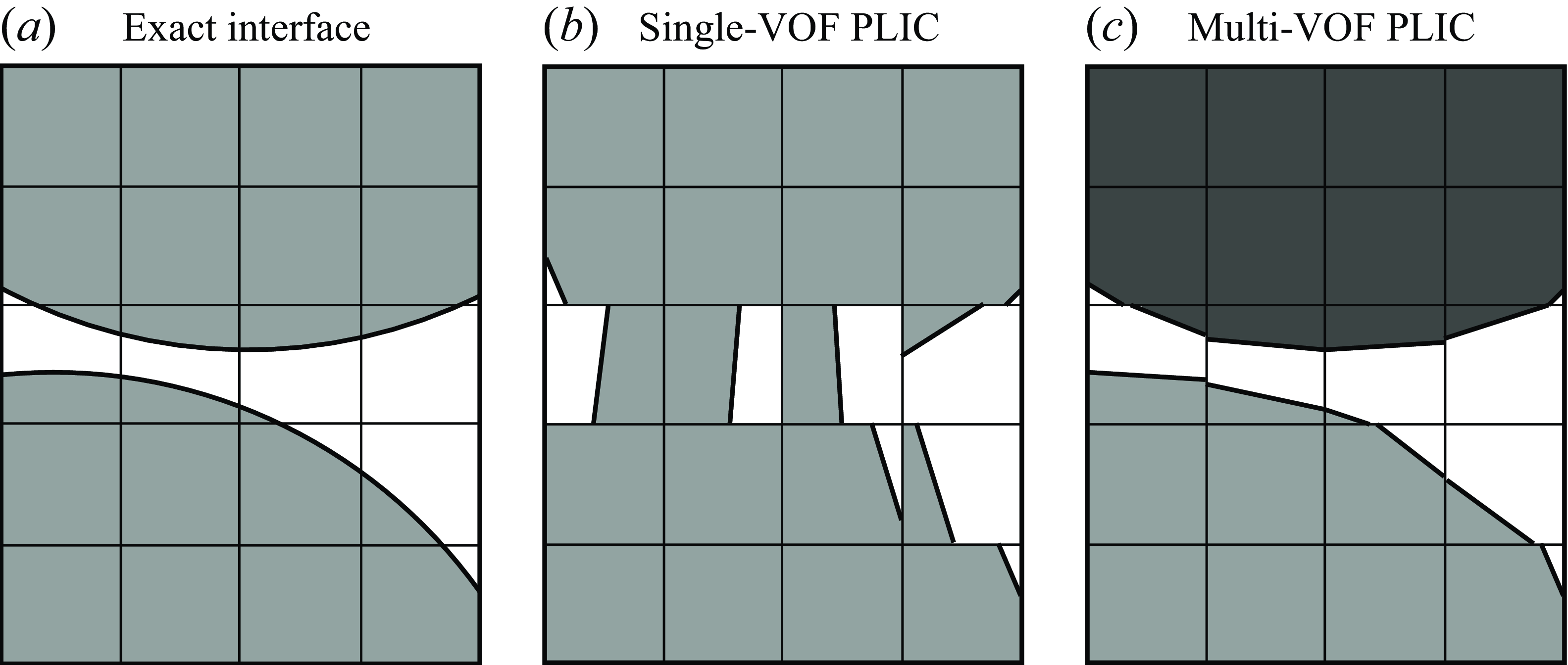
Illustration of numerical coalescence. (a) The exact interface of two close droplets is represented. (b) The PLIC reconstruction obtained from a single volume fraction field is illustrated. It is clear that the interfaces are not properly reconstructed and that PLIC can not allow two interface fragments in the same cell. (c) A PLIC reconstruction based on multi-VOF is shown where the interface is correctly reconstructed for both droplets.

3.1.1. Multi-VOF method
When using VOF to capture the interface, coalescence can be induced by numerical errors or lack of an appropriate subcell reconstruction of the interface. Usually, the merging of several interfaces occur when the resolution becomes too small (Boniou, Schmitt & Vié Reference Boniou, Schmitt and Vié2022) as illustrated in figure 2(b). Soligo et al. (Reference Soligo, Roccon and Soldati2019) demonstrated that this behaviour leads to an over-prediction of coalescence driven by the mesh size. In previous works on emulsions (Crialesi-Esposito et al. Reference Crialesi-Esposito, Rosti, Chibbaro and Brandt2022) and droplet-laden turbulence (Dodd & Ferrante Reference Dodd and Ferrante2016), the interface-capturing method was used without additional treatment and topology changes such as breakup and coalescence were allowed. In this work, it is more convenient to perform simulations at a fixed number of droplets of constant size for accumulating collision statistics. Hence, the topology change driven by the mesh becomes an undesirable feature that cannot be avoided without adding a numerical treatment to prevent interface merging. One solution would be to use an adaptive mesh refinement to better capture the interfaces and avoid such situations. However, physical coalescence usually occurs at the molecular scale (several mean-free paths) and the required level of refinement would be prohibitive to simulate a large number of droplets. A more pragmatic approach is to introduce a multi-VOF method where each droplet is represented by its own colour function. An analogous methodology has been applied successfully for the simulation of bouncing droplets using the context of a conservative level-set method (Balcázar et al. Reference Balcázar, Lehmkuhl, Rigola and Oliva2015), called the multiple marker level-set method. With multi-VOF, a list of volume fraction fields
 ${\mathcal{F}}= \{ f_1, f_2, \ldots , f_{N_{\kern-1pt f}} \}$
is transported using the conservative algorithm of Weymouth & Yue (Reference Weymouth and Yue2010). The capillary force
 $\boldsymbol{f}_{\kern-1pt \sigma}$
is modelled by a balanced-force continuum-surface-force formulation (Francois et al. Reference Francois, Cummins, Dendy, Kothe, Sicilian and Williams2006) adapted to the multi-VOF method by summing the force computed from each individual field
 \begin{equation} \boldsymbol{f}_{\!\sigma} = \sigma \sum _{i=1}^{N_{\!f}}\kappa _i \boldsymbol{\nabla }f_i, \end{equation}
with
 $\kappa _i$
the curvature computed from the volume fraction field
 $f_i$
and
 $\kappa$
the curvature estimated from height functions (Popinet Reference Popinet2009). This capillary force has been validated against numerical simulations and experiments by Fintzi et al. (Reference Fintzi, Pierson and Popinet2024) for the case of a droplet impact on a liquid–liquid interface. In practice, the multi-VOF dynamically adjusts the number of volume fraction fields
 $N_{\kern-1pt f}$
at each time step to optimise the computational cost associated to their transport. This is done by employing connected component analysis (CCA) as detailed by Herrmann (Reference Herrmann2010), which corresponds to the tag.h algorithm of Basilisk (Tomar et al. Reference Tomar, Fuster, Zaleski and Popinet2010). The tag field obtained from this algorithm is then used to detect overlapping droplets and to associate them to different volume fraction field. In two dimensions, the maximum number of fields is four to avoid overlapping droplets according to the four colour map theorem (Appel & Haken Reference Appel and Haken1977). In three dimensions, it was found in the numerical simulations presented in this work that this number never exceeds six (see Appendix A for details). Hence,
 $N_{\kern-1pt f}$
does not generally coincide with the number of droplets in the simulation which limits the over-cost of multi-VOF compared with the standard VOF algorithm.
3.1.2. Turbulence forcing
The turbulence is injected and maintained in the simulation by the volume force
 $\boldsymbol{f}_{\!T}$
. In this work a linear forcing in the fashion of Lundgren (Reference Lundgren2003) is used. In the recent study of Boniou et al. (Reference Boniou, Jay, Vinay and Pierson2025), it was shown that constant-energetics linear forcing methods of Bassenne et al. (Reference Bassenne, Urzay, Park and Moin2016) extended to two-phase flows allows us to recover the expected energy cascade of droplet-laden turbulence. It reads
 \begin{equation} \boldsymbol{f}_{\!T} = A\rho \boldsymbol{u}^{\prime} - \langle \boldsymbol{f}_{\kern-1pt \sigma} \rangle, \end{equation}
with
 $A$
the forcing magnitude defined by the constant-
 $k\epsilon$
method of Boniou et al. (Reference Boniou, Jay, Vinay and Pierson2025) and
 $\boldsymbol{u}^{\prime}=\boldsymbol{u}-\langle \boldsymbol{u}\rangle$
the fluctuating velocity vector in the one-fluid formulation. Hence,
 $\boldsymbol{f}_{\!T}$
is applied to the whole domain (both in carrier and dispersed phases). The mean part of the capillary force
 $\langle \boldsymbol{f}_{\kern-1pt \sigma} \rangle$
is removed in the fashion of Yao & Capecelatro (Reference Yao and Capecelatro2021) to prevent deviations of the mean flow and avoid exponential growth of kinetic energy observed in previous works (Naso & Prosperetti Reference Naso and Prosperetti2010; Chouippe & Uhlmann Reference Chouippe and Uhlmann2015). A comparison with an Arnold–Beltrami–Childress (ABC) forcing is presented in Appendix B.1 to study the impact of this turbulence forcing method on the collision statistics.
3.1.3. Should subgrid modelling of the lubrication force be included in the present simulations?
In this paper we do not include any subgrid lubrication model beyond the dynamics resolved on the current computational grid. While lubrication forces are known to play a significant role in the motion of solid particles in the Stokes flow regime (Durlofsky, Brady & Bossis Reference Durlofsky, Brady and Bossis1987), their applicability to inertial collision dynamics is debatable. Lubrication theory assumes that the collisional Reynolds number is much smaller than the ratio of particle diameter to film thickness (Leal Reference Leal2007). Under such conditions, inertia can be neglected, but this requires an accurate resolution of the thin-film flow up to the point where viscous forces begin to dominate. Moreover, when inertia dominates within the thin film, the lubrication singularity is likely to be much weaker than in the viscous-dominated case, further questioning the relevance of viscous-dominated lubrication models for inertia-dominated collisions (Miloh Reference Miloh1977; Pierson Reference Pierson2025).
The situation is qualitatively different for fluid particles. First, the force singularity during viscous droplet collisions is weaker than that for solid spheres (Davis, Schonberg & Rallison Reference Davis, Schonberg and Rallison1989). More importantly, fluid particles are deformable. When the pressure in the thin film approaches the capillary pressure, deformation is expected to occur. As a result, no true lubrication force singularity arises – instead, capillary forces become dominant. We now proceed to a more quantitative description of this behaviour. Assuming a high collisional Reynolds number – which is typically the case when
 $d \gg \eta$
– the pressure within the thin film between two colliding spherical droplets scales as
 $p \sim \rho _c w_r^2 d / h$
, where
 $h$
is the film thickness at the centreline between the droplets centres of mass (Pierson Reference Pierson2025). Although pressure is inversely proportional to the film thickness, the velocity of the droplets changes slightly during the initial stages of the collision, while they remain approximately spherical (see § 2.5). Given that the relative velocity scales as
 $w_r \sim (d\epsilon )^{1/3}$
, inserting this estimate into the pressure expression yields
 $p \sim \rho _c \epsilon ^{2/3} d^{5/3} / h$
. Assuming significant deformation occurs when the pressure in the thin film becomes comparable to the capillary pressure
 $\sigma / d$
, one obtains
 \begin{equation} \frac {h_c}{d} \sim {\textit{We}}, \end{equation}
where
 $h_c$
denotes the critical film thickness beyond which significant deformation is expected. Then, deformation becomes relevant when the film thickness is of the order of the Weber number. In the present case, significant deformation is expected for
 $h_c/d\sim 0.25$
, a thickness that is already well resolved by the current computational mesh (note that there are at least 30 cells per droplet diameter). Therefore, it is not necessary to include a subgrid lubrication force. (In this analysis, viscous effects within the film have been neglected. This assumption holds as long as the collisional Reynolds number, defined as
 ${\textit{Re}}_c = \rho _c d w_r/\mu$
is much smaller than
 $d/h$
(Leal Reference Leal2007). Then, when
 ${\textit{Re}}_c = \rho _c d w_r/\mu \sim d/h$
, viscous effects become significant. Using an inertial scaling for the relative velocity, the collisional Reynolds number may be expressed as
 ${\textit{Re}}_c \sim (d/\eta )^{4/3}$
. Then, within the current parameter range (see § 3.3), the film thickness at which viscous effects become non-negligible is
 $h/d \sim (d/\eta )^{-4/3} \approx 0.02$
, which is well below the deformation threshold. Thus, under these conditions, viscous effects can be safely neglected. However, at very low Weber numbers and for moderately high inertial collisions, a crossover between inertial and viscous scaling for the lubrication force may occur.) However, the question is whether the current simulation framework accurately predicts the capillary force between two droplets even when the intervening film is not resolved. The answer is yes – it does capture the capillary force correctly (Fintzi et al. Reference Fintzi, Pierson and Popinet2024), although there are certain effects not accounted for in the present analysis. Specifically, the film drainage process induces internal flow within the droplets (Davis et al. Reference Davis, Schonberg and Rallison1989), which cannot occur even when the film is not resolved. We believe that this internal flow is not sufficient to produce significant droplet deformation (i.e. normal stress differences), as long as
 ${\textit{We}} \ll 1$
. However, it alters the tangential boundary condition at the droplet interface. This effect could become relevant in dense droplet clusters, although it warrants further investigation.
3.2. Droplet post-processing
3.2.1. Droplet list from Eulerian fields
The collection of droplet statistics requires the explicit definition of a list of
 $N_d$
discrete droplet elements
 $\mathcal{D}= \{ D_1, D_2, \ldots , D_{N_d} \}$
as illustrated in figure 3(c). In point-particle and PR-DNS, the droplet population
 $\mathcal{D}$
is known a priori and the equations solved for the dispersed phase directly transport each droplet
 $D_i$
with position
 $\boldsymbol{y}_i$
and velocity
 $\boldsymbol{v}_i$
in a Lagrangian fashion (Wang et al. Reference Wang, Wexler and Zhou1998a
; Cate et al. Reference Cate, Andreas, Jos, Portela, Van Den and Harry2004). An interface-capturing method does not explicitly transport the list of droplets but a list of volume fraction fields, which is indirect information on the droplet positions. Hence, a detection procedure is required to convert the continuous representation of the dispersed phase into a list of discrete elements
 $\mathcal{D}$
.
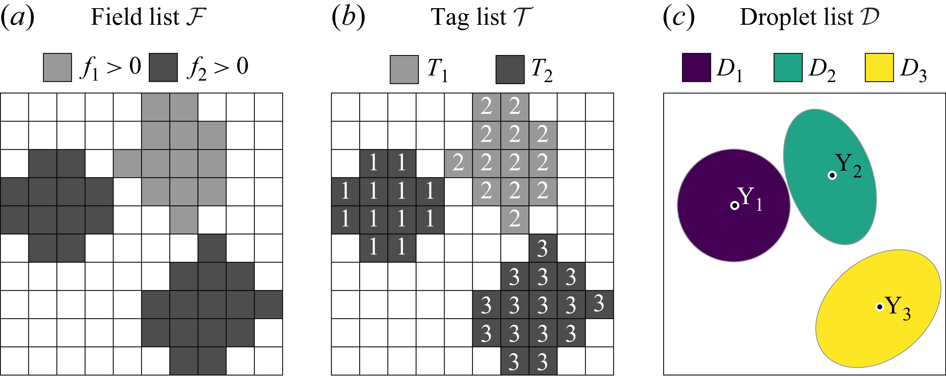
Illustration of (a) the field list
 ${\mathcal{F}}$
, (b) the tag list
 $\mathcal{T}$
and (c) the droplet list
 $\mathcal{D}$
on a minimal case in two dimensions. The values of the tag fields are written directly in the corresponding cells in panel (b) and the droplet centres
 $\boldsymbol{y}_i$
are represented in panel (c).

Sampling discrete droplet elements from an Eulerian field is a classic procedure in various applications such as atomisation (Desjardins et al. Reference Desjardins, McCaslin, Owkes and Brady2013), emulsion (Crialesi-Esposito, Chibbaro & Brandt Reference Crialesi-Esposito, Chibbaro and Brandt2023) or wave breaking (Riviere et al. Reference Riviere, Mostert, Perrard and Deike2021). The CCA algorithm evoked in § 3.1.1 is used to obtain a tag field
 $T$
that attributes to each computational cell a number that corresponds to the discrete element it belongs to. In the specific case of multi-VOF, a list of volume fraction fields
 ${\mathcal{F}}$
needs to be treated instead of a single field. Then, the CCA algorithm needs to be applied on each volume fraction field
 $f_i$
to obtain an intermediate list of tag fields
 $\mathcal{T}= \{ T_1, T_2, \ldots , T_{N_{\kern-1pt f}} \}$
of size
 $N_{\kern-1pt f}$
. These two lists are illustrated in figures 3(a) and 3(b) where a minimal example is provided. The tag list is used to define a Dirac function
 $\delta ^T_{{\textit{i},\textit{j},\textit{k}}}$
that is only
 $1$
when the computational cell
 $k$
containing a part of droplet
 $D_i$
is accounted for in the integration, i.e.
 \begin{equation} \delta ^T_{{\textit{i},\textit{j},\textit{k}}} = \begin{cases} 1, & \text{if $i = T_{j,k}$},\\ 0, & \text{otherwise}, \end{cases} \end{equation}
with
 $T_{j,k}$
the tag field computed from the VOF field
 $f_j$
at cell
 $k$
.
The last step is to compute the quantities associated to each droplet in the droplet list. The position
 $\boldsymbol{y}_i$
and velocity
 $\boldsymbol{v}_i$
for the
 $i$
th droplet are retrieved by volume integration on the droplet volume
 $V_i$
:
 \begin{equation} \boldsymbol{y}_i = \int _{V_i} \boldsymbol{x} {\textrm{d}}v, \quad \boldsymbol{v}_i = \int _{V_i} \boldsymbol{u} {\textrm{d}}v. \end{equation}
In opposition to point-particle and PR-DNS approaches, the simulations performed in this work also capture the internal flow in the droplet and the deformation of the interface. Hence, it is useful to introduce a general quantity of interest
 $q$
obtained from volume or surface integration on the droplet
 $D_i$
:
 \begin{align} q^v_i = \int _{V_i} q {\textrm{d}}V &= \sum _{j=0}^{N_{\kern-1pt f}} \sum _{k=0}^{N_\varDelta } \delta ^T_{{\textit{i},\textit{j},\textit{k}}}f_{j,k}q_{k}\Delta v_{k}, \end{align}
 \begin{align} q^s_i = \int _{S_i} q {\textrm{d}}S &= \sum _{j=0}^{N_{\kern-1pt f}} \sum _{k=0}^{N_\varDelta } \delta ^T_{{\textit{i},\textit{j},\textit{k}}}\varSigma _{j,k}q_{k}\Delta v_{k}. \end{align}
Here
 $S_i$
is the the surface associated to droplet
 $D_i$
,
 $N_\varDelta$
is the number of cells in the computational domain,
 $\Delta v_{k}$
is the volume of cell
 $k$
,
 $\varSigma _{j,k}$
is the surface density of the interface computed from
 $f_j$
in cell
 $k^{\prime}$
.
The collision detection not only requires the knowledge of the droplet properties at the current time
 $t^n$
but also the history of the droplet in previous times. This is done using an algorithm detailed in Appendix A to obtain a list of droplets
 $\mathcal{D}^n$
for each time frame with corresponding position, velocity and additional properties if required (surface, hydrodynamic forces, kinetic energy, etc.).
3.2.2. Contact definition
When deformable droplets are involved, contact cannot be defined by the separating distance between droplet centroid. In such a case, two droplets separated by a distance
 $d$
, or smaller, are not necessarily in contact depending on their deformation. In the simulations, the droplets are never spherical due to the flow–droplet and droplet–droplet interactions as demonstrated in § 4.4. Also, droplets can still be in contact even though the distance between their centre of mass is higher than
 $d$
. In the simulations, the contact criterion is based on the PLIC reconstruction that provides the barycentre
 $\boldsymbol{x}_{\varGamma ,k,i}$
and surface
 $S_{\varGamma ,k,i}$
of an interface fragment
 $k$
belonging to droplet
 $D_i$
. The contact surface
 $S_{{\textit{c},\textit{ij}}}$
of droplet
 $D_i$
with droplet
 $D_j$
is computed as
 \begin{equation} S_{{\textit{c},\textit{ij}}} = \sum _{k}^{N_{\varGamma ,i}} \chi _{k,\textit{ij}}S_{\varGamma ,k,i}, \end{equation}
with
 $\chi _{k,\textit{ij}}$
an indicator function that is only
 $1$
when the distance between the interface of droplets
 $D_i$
and
 $D_j$
is smaller than the mesh size
 $\Delta x$
: i.e. a fragment of interface with barycentre
 $\boldsymbol{x}_{\varGamma ,k,i}$
, belonging to
 $D_i$
, has at least one fragment of interface with barycentre
 $\boldsymbol{x}_{\varGamma ,l,j}$
, belonging to droplet
 $D_j$
, such that
 $\lvert \boldsymbol{x}_{\varGamma ,k,i} - \boldsymbol{x}_{\varGamma ,l,j} \rvert \lt \Delta x$
. Note that discretely
 $S_{{\textit{c},\textit{ij}}}$
does not necessarily correspond to
 $S_{c,ji}$
and the contact criterion is then defined as
 $\min (S_{{\textit{c},\textit{ij}}},S_{c,ji}) \gt \Delta x^2$
with
 $\Delta x^2$
a small threshold to remove parasitic contact. Even if this criterion depends on
 $\Delta x$
, it is demonstrated in Appendix B.2 that the mesh size does not impact the results of the simulations.
3.2.3. Collision detection
We define a collision event as an event in which a pair of droplets start to touch each other and separate after a contact time. To avoid keeping track of the history of each pair of droplets, the number of collisions can rely on the number of simultaneous contacts. The number of simultaneous contacts
 $N_{sc,i}^n$
of each droplet
 $D_i$
at a time
 $t^n$
is computed as
 \begin{equation} N_{sc,i}^n = \sum _{j\neq i}^{N_d} H\big(S_{{\textit{c},\textit{ij}}}^n\big), \end{equation}
with
 $H$
the Heaviside function. The collision event is composed of two steps: first the droplets are in contact and then they come apart. From this observation, a collision can be recorded when
 $N_{sc,i}$
changes value during a time step
 $\Delta t$
. If the sampling frequency is small enough, this method can capture all the collision events. Hence, the total number of collisions for
 $N_d$
droplets during
 $N_t$
time steps of a simulation is
 \begin{equation} N_c = \frac {1}{2}\sum _{n=1}^{N_t}\sum _{i=1}^{N_d}\max {\left (0,\Delta N_{sc,i}^n\right )}, \end{equation}
with
 $\Delta N_{sc,i}^n = N_{sc,i}^n - N_{sc,i}^{n-1}$
the instantaneous variation of
 $N_\textit{sc}$
for droplet
 $i$
at time
 $t^n$
. The result is divided by two in order to cancel the double counting of collisions for each pair.
The dynamic collision kernel is then computed as (Zhou, Wexler & Wang Reference Zhou, Wexler and Wang1998)
 \begin{equation} \varGamma = \frac {2V_\varOmega N_c}{t_f N_d^2}, \end{equation}
with
 $t_f$
the final time of the simulation.
3.2.4. Sampling frequency
Collision events happen during a finite time (Chesters Reference Chesters1991) approximated by (2.35). By injecting the definition of
 ${\textit{We}}=\rho _c\epsilon ^{2/3}d^{5/3}/\sigma$
in (2.35) with
 $\rho _r=1$
we obtain
 $t_c \sim \sqrt {{\rho _c d^3}/{\sigma }}$
. This estimate can be compared with the capillary time-step constraint used in the simulations
 $\Delta t = \sqrt {{\rho _c \Delta x^3}/{\sigma }}$
, ensuring that the capillary waves of size
 $\Delta x$
are temporally captured, which gives
 $t_c/\Delta t \sim (d/\Delta x)^{3/2}\sim 30^{3/2} \gt 10^2$
.
The main part of the collisions should happen in a time interval larger than
 $\Delta \tau$
to ensure the temporal resolution of collision events in post-processing. As droplet sampling is expensive, the sampling frequency of droplet lists
 $1/\Delta \tau$
should be as small as possible. Hence,
 $\Delta \tau$
might be chosen small enough such that it captures collisions but large enough so that the simulation is not slowed down by on-the-fly post-processing:
 $\Delta t\lt \Delta \tau \lt t_c$
. In this work, numerical experiments showed that
 $\Delta \tau = t_c/50$
achieved temporal convergence.
3.3. Flow configuration
The numerical simulations presented in this work consist of a periodic box of length
 $\mathcal{L}=2\pi$
filled with droplets in a turbulent flow to mimic a liquid–liquid emulsion. The turbulent carrier phase is characterised by the root-mean-square fluctuation velocity
 $u^{\prime}$
, the dissipation rate
 $\epsilon$
and the integral length scale
 $\ell$
. The turbulent flow is defined by the Reynolds number
 ${\textit{Re}}_\lambda = u^{\prime}\lambda /\nu _c$
based on the Taylor microscale
 $\lambda =\sqrt {15\nu _c/\epsilon }\,u^{\prime}$
and the kinematic viscosity
 $\nu _c=\mu _c/\rho _c$
. The particularity of the numerical set-up is the direct relation
 $\ell \sim 0.19\mathcal{L}$
resulting from the linear forcing of turbulence (Rosales & Meneveau Reference Rosales and Meneveau2005). The integral length is then fixed by the domain size and will remain the same for all simulations even with droplets.
For the dispersed phase, the droplet population is monodisperse with diameter
 $d$
and volume fraction (hold-up)
 $\varPhi$
. The dynamic of the dispersed phase is driven by the Weber number
 ${\textit{We}}$
that is fixed to 0.25 to prevent droplet breakup and keep a population with constant numbers and size. This feature remains true only if the coalescence is prevented numerically by the multi-VOF algorithm presented in § 3.1. The droplet size relevant to our application lies in the inertial regime of turbulence where
 $d/\eta \gt 1$
with the Kolmogorov length scale
 $\eta = (\nu _c^3/\epsilon )^{1/4}$
. The problem is also governed by the density ratio
 $\rho _r$
and the viscosity ratio
 $\mu _r$
. The choice of these physical parameters is constrained by the resolution requirements from turbulence and droplet scales. The first mesh criterion is based on the Kolmogorov scale
 $\eta$
that gives
 $\Delta x \lt 1.5\eta$
(Eswaran & Pope Reference Eswaran and Pope1988). The second mesh criterion is the required number of cells in the diameter of a droplet to capture the interface. Usually, the minimum number of cells in the diameter is around
 $30$
to provide an acceptable interface dynamic. In the work of Dodd & Ferrante (Reference Dodd and Ferrante2016) who investigated Taylor-size droplets in turbulence,
 $32$
cells in the droplet diameter appears to be a good compromise between accuracy and computational cost. In this work, all the calculations are conducted on a uniform grid of
 $512^3$
cells such that
 $\kappa _{\textit{max}}\gt 1.5\eta$
and the droplet resolution is
 $d \gt 32\Delta x$
for the worst case
 $d=15\eta$
. A simulation with
 $256^3$
cells is also presented in Appendix B.2 to verify mesh convergence of the simulations.
The simulations are setup as follows: (i) first, a baseline single-phase HIT simulation S0 is run for a sufficiently long time,
 $50\tau _\ell$
with
 $\tau _\ell = u^{{\prime}2}/\epsilon$
the integral time scale such that the flow is statistically converged; (ii) next, the droplet-laden HIT simulation is initialised by restarting from S0, replacing the carrier phase at random locations with the droplet phase, but keeping the velocity field unchanged; (iii) finally, the simulation undergoes a transient period where kinetic energy is exchanged between the phases, eventually reaching a stationary regime in which statistically converged data can be collected. The two-phase simulations are run during
 $25\tau _\ell$
and we start computing statistics after
 $5\tau _\ell$
. Statistical convergence of the baseline two-phase simulation S1 is assessed in Appendix B.3.
The numerical simulations used in the result section are summed up in table 1 and illustrated in figure 4. The main parameters are
 ${\textit{We}} = 0.25$
,
 ${\textit{Re}}_\lambda = 48.6$
,
 $\nu _c =0.005$
,
 $\rho _r = 1$
and
 $\mu _r = 1$
with varying droplet size (
 $d/\eta = \{15,20,25\}$
) and volume fraction (
 $\varPhi = \{6\,\%,18\,\%\}$
). Additionally, two simulations are run with modified droplet properties: one with more viscous droplets (
 $\mu _r = 10$
) and another with denser droplets (
 $\rho _r = 2$
). Finally, a simulation with
 ${\textit{Re}}_\lambda = 80.1$
is also included to verify generality of the results with varying
 $\epsilon$
.
Physical set-up for the cases studied in this paper.

Snapshots for each simulation run of table 1. The droplets appear in colours that correspond to their number of simultaneous contacts
 $N_\textit{sc}$
defined by (3.12). The
 $\lambda _2$
criterion of Jeong & Hussain (Reference Jeong and Hussain1995) is also displayed on planes.

4. Results
4.1. Eulerian turbulent statistics
In two-phase flows the turbulence is modulated by droplets and it is interesting to study the averaged quantities in the simulations
 $\overline {k}$
,
 $\overline {\epsilon }$
and
 $\overline {S}_{ll}$
, which are defined as
 \begin{equation} \overline {k} = \frac {1}{2}\overline {\int _\varOmega \boldsymbol{u} \boldsymbol{\cdot }\boldsymbol{u} {\textrm{d}}V}, \quad \overline {\epsilon } = \overline {\int _\varOmega \nu \boldsymbol{\nabla }\boldsymbol{u} : \boldsymbol{\nabla }\boldsymbol{u} {\textrm{d}}V}, \quad \overline {S}_{ll}(r) = \overline {\left \langle \delta u_r^2\right \rangle }, \end{equation}
with
 $\int _\varOmega$
the spatial integral over the domain
 $\varOmega$
,
 $\overline { \;\boldsymbol{\cdot }\;}$
the temporal average and
 $\langle \delta u_r^2\rangle$
the longitudinal increment of
 $\boldsymbol{u}$
at an interval
 $r$
averaged over all fluid particles:
 \begin{align} \big\langle \delta u_r^2 \big\rangle = \frac {1}{3} &\big \langle \left (u_x(x+r,y,z) - u_x(x,y,z)\right )^2 \nonumber\\ + &\;\left (u_y(x,y+r,z) - u_y(x,y,z)\right )^2 \nonumber\\ + &\; \left (u_z(x,y,z+r) - u_z(x,y,z)\right )^2\big \rangle. \end{align}
As the modelling is based on the turbulent flow in the carrier phase, an additional analysis is performed by discriminating the carrier phase in the averages:
 \begin{equation} \overline {k}_c = \frac {1}{2}\overline {\int _{\varOmega _c} \boldsymbol{u} \boldsymbol{\cdot }\boldsymbol{u} {\textrm{d}}V}, \,\, \overline {\epsilon }_c = \overline {\int _{\varOmega _c}\nu \boldsymbol{\nabla }\boldsymbol{u} : \boldsymbol{\nabla }\boldsymbol{u} {\textrm{d}}V}, \,\, \overline {S}_{ll,c}(r) = \overline {\left \langle \delta u_{r,c}^2\right\rangle }.\end{equation}
Here
 $\int _{\varOmega _c}$
is the spatial integral over the carrier phase
 $\varOmega _c$
and
 $\overline {\langle \delta u_{r,c}^2\rangle }$
is the squared longitudinal increment of
 $\boldsymbol{u}$
at an interval
 $r$
averaged over fluid particles belonging to the carrier phase.
These quantities, normalised by the target values
 $k$
,
 $\epsilon$
and
 $({\textrm{d}}\epsilon )^{2/3}$
from the linear forcing technique, are provided in table 2 for all simulations. The mean Kolmogorov constants
 $\overline {C}_2$
and
 $\overline {C}_{2,c}$
are determined at a separation distance of
 $r=d$
(
 $r=20\eta$
for S0) using the values of the normalised longitudinal structure functions
 $\overline {S}_{ll}(d)/({\textrm{d}}\epsilon )^{2/3}$
and
 $\overline {S}_{ll,c}/({\textrm{d}}\epsilon )^{2/3}$
, respectively. It appears that the linear forcing can impose the target quantities
 $k$
and
 $\epsilon$
for all the simulations with deviations of about
 $5\,\%$
at maximum. In table 2 we can also observe that the difference between carrier-averaged and domain-averaged quantities is relatively small. Many studies on finite-size particles in turbulence examine the difference between the particle (here, droplet) velocity variance and the continuous phase velocity variance, expressed as
 $(\overline {k}_c-\overline {k}_d)/\overline {k}_c$
. This difference is expected to increase with increasing diameter and vanish in the tracer limit. Homann & Bec (Reference Homann and Bec2010) introduced a scaling law in
 $(d/\eta )^{2/3}$
for this velocity variance difference within the inertial range of turbulence. In figure 5 the literature data compiled by Uhlmann & Chouippe (Reference Uhlmann and Chouippe2017) is supplemented with the results from the present study and the particle simulations of de Motta et al. (Reference de Motta, Estivalezes, Climent and Vincent2016). As noted by Homann & Bec (Reference Homann and Bec2010) and Uhlmann & Chouippe (Reference Uhlmann and Chouippe2017), although the scaling law cannot be strictly satisfied at low Reynolds numbers due to the limited extent of the inertial range, it is, nevertheless, recovered. Our simulation results appear to be consistent with other particle-laden turbulence simulations, confirming the robustness of this trend across a broad range of flow conditions. These include cases spanning from a single neutrally buoyant (
 $\rho _r=1$
) particle at low Reynolds number (
 ${\textit{Re}}_\lambda =32$
) studied by Homann & Bec (Reference Homann and Bec2010), to more complex scenarios such as moderately dense (
 $\varPhi =6\,\%$
) suspensions of neutrally buoyant (
 $\rho _r=1$
) or denser (
 $\rho _r=1.4$
) particles at higher Reynolds number (
 ${\textit{Re}}_\lambda =60$
) investigated by Yeo et al. (Reference Yeo, Dong, Climent and Maxey2010). Further supporting this trend are studies on dilute suspensions (
 $\varPhi =0.5\,\%$
) of neutrally buoyant (
 $\rho _r=1$
) or denser (
 $\rho _r=1.5$
) particles at
 ${\textit{Re}}_\lambda \approx 60$
by Chouippe & Uhlmann (Reference Chouippe and Uhlmann2015) and Uhlmann & Chouippe (Reference Uhlmann and Chouippe2017), as well as moderately dense (
 $\varPhi =3\,\%$
) suspensions of neutrally buoyant (
 $\rho _r=1$
) or heavier (
 $\rho _r=2$
) particles at
 ${\textit{Re}}_\lambda = 73$
from de Motta et al. (Reference de Motta, Estivalezes, Climent and Vincent2016). Additionally, it aligns with the results for neutrally buoyant (
 $\rho _r=1$
) particles at
 ${\textit{Re}}_\lambda \approx 130$
studied by Cisse, Homann & Bec (Reference Cisse, Homann and Bec2013).
Temporal mean of turbulent quantities measured from the simulations. Here
 $\overline {C}_2$
is computed as
 $\overline {S}_{ll}/(r\epsilon )^{2/3}$
at the distance
 $r=20\eta$
for S0, S1, S2, S3 and S4,
 $r=15\eta$
for S5 and
 $r=25\eta$
for S0’, S6 and S6’ corresponding to the diameter of the droplets.

Difference between the variance of the fluid velocity and the particle velocity (
 $(\overline {k}_c-\overline {k}_d)/\overline {k}_c$
). The symbols correspond to: Homann & Bec (Reference Homann and Bec2010) (
 , blue); Yeo et al. (Reference Yeo, Dong, Climent and Maxey2010) (
 , blue for
 $\rho _r=1$
and orange for
 $\rho _r=1.4$
); Chouippe & Uhlmann (Reference Chouippe and Uhlmann2015) (
 , blue); Uhlmann & Chouippe (Reference Uhlmann and Chouippe2017) (
 , orange); de Motta et al. (Reference de Motta, Estivalezes, Climent and Vincent2016) (
 , blue for
 $\rho _r=1$
and orange for
 $\rho _r=2$
); Cisse et al. (Reference Cisse, Homann and Bec2013) (
 ); present simulations (
 ). The scaling
 $\propto d^{2/3}$
is also included (
 ).

Longitudinal structure function
 $\overline {S}_{ll}$
for the single-phase and droplet-laden case and
 $\overline {S}_{ll,c}$
for the droplet-laden case for S0/S1 (
 ${\textit{Re}}_\lambda = 48.6$
) (a) and S0’/S6’ (
 ${\textit{Re}}_\lambda = 80.1$
) (b). The inset figures show a close-up of the structure function in the range
 $r=[10\eta ,30\eta ]$
.

Regarding the scale-by-scale characteristic of the turbulence, it is clear in figure 6 that the Kolmogorov constant
 $C_2$
is lower than the asymptotic value at infinite Reynolds numbers (approximately 2) and depends on
 ${\textit{Re}}_\lambda$
. It is important to note that for the small Reynolds number considered here, the inertial subrange of turbulence is relatively narrow, and a long plateau cannot be observed in the structure function as evidenced in the inset graph of figures 6(a) and 6(b), even if a longer plateau is observed for
 ${\textit{Re}}_\lambda =80.1$
. Hence, a difference of
 $5\,\%\!-\!10\,\%$
is observed for S1, S5 and S6 in terms of
 $\overline {C}_2$
as they are computed from
 $\overline {S}_{ll}/(r\epsilon )^{2/3}$
at different
 $r=20\eta$
,
 $15\eta$
and
 $25\eta$
, respectively. For the variation with
 ${\textit{Re}}_\lambda$
, an increase of about
 $20\,\%$
is observed from
 ${\textit{Re}}_\lambda =48.6$
to
 ${\textit{Re}}_\lambda =80.1$
. Note that the resulting scaling of
 $C_2$
in
 $\epsilon$
is quite small as
 ${\textit{Re}}_\lambda =48.6 \rightarrow \epsilon =0.24$
and
 ${\textit{Re}}_\lambda =80.1 \rightarrow \epsilon =4.8$
, which leads to the power law
 $\varLambda =\log ({1.5/1.3})/\log ({4.8/0.24})\approx 0.05$
based on the two points tested here. This result is in accordance with the experimental study of Ni & Xia (Reference Ni and Xia2013). For the remaining part of the results,
 $\overline {C}_2=1.3$
is used as a reference for simulations with
 ${\textit{Re}}_\lambda =48.6$
and
 $\overline {C}_2=1.5$
for simulations with
 ${\textit{Re}}_\lambda =80.1$
. We also observe that the longitudinal structure function exhibits little difference between the single-phase flow simulation and the two-phase flow simulation. Furthermore, its values remain largely unaffected by the computation method, whether evaluated over both phases or exclusively within the continuous phase. Hence, as assumed in §§ 2.4–2.6, we may expect the same properties of the inertial range of turbulence, i.e. negligible viscous effects in both single-phase and two-phase flow simulations.
4.2. Non-binary contacts
A key assumption in deriving the collision rate in § 2 is that collisions are instantaneous and binary. This requires the mean contact time to be much shorter than the mean time between successive collisions. Under this assumption, pairwise interactions are the most likely to occur and are considered to be the main statistical collision events. As the mean-free time, which is the inverse of the collision rate, scales as
 $\varPhi ^{-1}$
(see (2.34)), we can expect this assumption to be true only in the dilute regime.
Effect of droplet volume fraction on non-binary contacts.

In simulations involving finite-size droplets with a moderate volume fraction (ranging between
 $1\,\%$
and
 $20\,\%$
), the regime is no longer considered dilute (Sommerfeld Reference Sommerfeld2017), and interactions may involve more than two droplets. An indicator of such multi-droplet interactions is the number of simultaneous contacts on a droplet, as defined in (3.12). From the list of droplets in contact, it is also possible to define aggregates of
 $m$
droplets in connected contact. By recursively seeking droplets in contact with each other, it is possible to reconstitute all aggregates at a given time. From an ensemble perspective, an aggregate list of
 $m$
connected droplets
 $\mathcal{A}= \{A_1,\ldots ,A_{N_A} \}$
is then defined.
In the dilute regime, we may expect the aggregates
 $A_i$
to be only single droplets (
 $m=1$
and
 $N_\textit{sc}=0$
) or pairs of droplets (
 $m=2$
and
 $N_\textit{sc}=1$
). In figure 7(a) the probability
 $P(N_\textit{sc})$
of having
 $N_\textit{sc}$
over all time and droplets is given. Even for S1 (
 $\varPhi =6\,\%$
),
 $P(N_\textit{sc}=2)$
is higher than
 $1\,\%$
. For S4 (
 $\varPhi =18\,\%$
), the probability for a droplet to be in contact is higher than being single and
 $P(N_\textit{sc}=5)\gt 0$
. In figure 7(b) the probability
 $P(m)$
of having aggregates of size
 $m$
over all time is also provided. Aggregates of size
 $7$
for S1 (
 $\varPhi =6\,\%$
) and more than
 $20$
for S4 (
 $\varPhi =18\,\%$
) can be reached. Hence, many droplets can be simultaneously interconnected. The results for other simulations at
 $\varPhi =6\,\%$
show a similar trend.
4.3. Contact time
As discussed in § 2.6, the contact time is expected to be finite in the simulations. The dimensionless mean contact time
 $t_c$
is displayed as a function of
 $d/\eta$
for all the simulations in figure 8. In the simulations the mean contact time remains approximately constant as a function of
 $d/\eta$
for S5, S1 and S6 (
 $d/\eta =15,20,25$
). This confirms that with a fixed Weber number, the eddy turnover time is a reliable scaling law for the mean contact time, as predicted by (2.35). However, the measured contact time is greater than the theoretical prediction. This discrepancy can be explained by the various assumptions made in the model: instantaneous deformation and inviscid collision. Simulation S2 (
 $\rho _r=2$
) also shows an increase in the contact time in agreement with (2.35). Finally, the effect of viscosity and volume fraction also increases the contact time. These observations would suggest that a complete model for the contact time during a collision should also include both
 $\varPhi$
and
 $\mu _r$
, although the effect of those parameters is small.
Mean contact time
 $t_c$
normalised with the turnover eddy time
 $d^{2/3}\epsilon ^{-1/3}$
as a function of
 $d/\eta$
for all the simulations. The value corresponding to (2.35) with
 $\rho _r=1$
(
 ) and
 $\rho _r=2$
(
 ) is also provided as a reference.

4.4. Droplet shape
In § 2 we assume that the droplets are spherical, which requires the Weber number to be much smaller than one. We compute the sphericity
 $\mathcal{S}_p$
and aspect ratio
 $\chi$
of the droplets to verify this approximation. The definitions of the sphericity and aspect ratio are taken from the work of Cannon, Soligo & Rosti (Reference Cannon, Soligo and Rosti2024). The sphericity
 $\mathcal{S}_p$
is defined as the ratio between the volume-equivalent diameter
 $d$
and the surface-based diameter
 $d_S=\sqrt {S/\pi }$
. The aspect ratio is based on the inertia tensor, such that
 \begin{equation} \boldsymbol{I} = \int _{V_d} \big(r_c^2\boldsymbol{\delta } - \boldsymbol{r}_c \otimes \boldsymbol{r}_c \big)\, {\textrm{d}}v, \end{equation}
where
 $V_d$
is the droplet volume,
 $\boldsymbol{\delta }$
the identity tensor and
 $\boldsymbol{r}_c = \boldsymbol{x}-\boldsymbol{y}$
the distance to the centroid of the droplet
 $\boldsymbol{y}$
defined by (3.8). Eigenvalues
 $\lambda _1,\lambda _2,\lambda _3$
of
 $\boldsymbol{I}$
provides the three semi-axes of an ellipsoid
 $a_1$
,
 $a_2$
,
 $a_3$
. For a perfect sphere,
 $a_i=d/2$
and eigenvalues
 $\lambda _i$
are related to
 $a_i$
with the expression
 $\lambda _i=2a_i^2/5$
. An example of evolution of the three eigenvalues
 $\lambda _i$
is given for a droplet during
 $10\tau _\ell$
in figure 9. It clearly shows that the droplet deforms with a variation of
 $\pm 5\,\%$
around the equivalent sphere diameter
 $d$
. The aspect ratio is defined as
 $\chi =\sqrt {\lambda _{\textit{min}}/\lambda _{{\textit{max}}}}$
such that both metrics
 $\mathcal{S}_p$
and
 $\chi$
take values in the range
 $[0,1]$
with
 $1$
being the value for a perfect sphere.
Evolution of the three eigenvalues
 $\lambda _i$
normalised by
 $\sqrt {10}/d$
for a single droplet during a time frame of
 $10\tau _\ell$
for simulation S1.

In figure 10 the average over all droplets and all time of sphericity
 $\langle \mathcal{S}_p\rangle$
with respect to the aspect ratio
 $\langle \chi \rangle$
is given for all the simulations with an ellipse representing the standard deviation around the mean. None of the mean droplet shapes observed in the simulations follow the ellipsoidal description, as their sphericity is lower than that of an ellipsoid. This suggests that the droplet areas are increased due to small-scale perturbations of the interface. Overall, the deformation of the drops from their spherical shape remains limited, with aspect ratio variations below
 $10\,\%$
and sphericity deviations under
 $1 \,\%$
.
Mean sphericity
 $\langle \mathcal{S}_p\rangle$
with respect to the mean aspect ratio
 $\langle \chi \rangle$
for all the simulations. The analytical relation between sphericity and aspect ratio of an ellipsoid is also included (
). The marker’s size in (b) is proportional to the diameter (small:
 $d/\eta =15$
, medium:
 $d/\eta =20$
and large:
 $d/\eta =25$
).

Near the critical Weber number predicted by KH theory, deformations arise from both turbulence-induced pressure on the droplet and interactions between droplets. For S4 with a high volume fraction (
 $\varPhi =18\,\%$
), the droplet–droplet interactions are dominant, which increase the mean deformation of the droplets compared with S1 (
 $\varPhi =6\,\%$
). Simulation S3 with viscous droplets (
 $\mu _r=10$
) shows a decrease in deformation, most probably due to the increase of droplet energy dissipation during contact with less kinetic energy transferred into surface energy. Another possible explanation comes from the viscous normal stress within the droplet, which could resist deformation upon contact. To test this hypothesis, we calculate the Capillary number,
 ${\textit{Ca}} = \mu _d (\epsilon d)^{1/3}\gamma$
, using the droplet internal viscosity and inertial velocity scales. Since the droplet Reynolds number is approximately
 $d/\eta$
(with the Reynolds number for Kolmogorov eddies being close to one), we find that
 ${\textit{Ca}} \sim {\textit{We}} \mu _r \eta /d = 0.125$
. The normal stress during contact can be considered negligible for this viscosity ratio, though it may become significant for a larger viscosity ratio. For S2, characterised by denser droplets (
 $\rho _r=2$
), a significant increase in deformation is observed. This finding aligns with expectations due to the greater inertia of the droplets. Indeed, in the original model of Chesters & Hofman (Reference Chesters and Hofman1982), Chesters (Reference Chesters1991), the energy of the droplet and continuous phase is converted exclusively into capillary energy. Consequently, a higher droplet density ratio results in greater kinetic energy upon collision (assuming the droplet velocity remains given by the eddy velocity of size
 $d$
), thereby enhancing the deformation during the collision. The effect of droplet properties are even more visible in figure 11 where points are way more scattered far from the spherical shape for S2 than S1 while points are more concentrated around the spherical shape for S3. For S6’, deformation is increasing with the Reynolds number (
 ${\textit{Re}}_\lambda =80.1$
), which reinforced the idea of small-scale perturbations increasing the area of the droplets. Finally, the droplet size does not have a strong impact on deformation even if the deformation seems to increase with droplet size.
Effect of droplet properties – S1 (a), S2 (b) and S3 (c) – on the scatter plot of mean sphericity
 $\langle \mathcal{S}_p\rangle$
with respect to the mean aspect ratio
 $\langle \chi \rangle$
. Each point corresponds to a droplet
 $D_i$
at an instant
 $t$
.

4.5. Radial distribution function
In § 2 we presented two models for the RDF corresponding to hard spheres and soft spheres governed by an inverse-power-law potential. They should both depend on
 $\varPhi$
in moderately dense regimes where geometric effects act on the value of RDF with a peak close to
 $r=d$
.
In figure 12 the RDF obtained from S1 (
 $\varPhi =6\,\%$
) and S4 (
 $\varPhi =18\,\%$
) are compared with the hard-sphere model and the soft-sphere model with
 $n=4$
(2.21). Due to deformation, the RDF takes finite positive values for
 $r\lt d$
and increases with
 $r$
, suggesting that smaller separation distances – corresponding to higher deformations – are less likely to occur. In the range
 $r\gt d$
, the RDF increases up to approximately
 $1$
with a bump at
 $r=d$
similar to hard spheres. However, this local maximum remains below the analytical value predicted by the hard-sphere model (2.18) even if the value of this maxima increases slightly with the volume fraction in figure 12(b). Additionally, the RDFs for droplets in contact and those without contact are shown as inset graphs in figures 12(a) and 12(b). These RDFs are defined based on the probability of a droplet pair being in contact (
 $P(S_c\gt 0)$
) as
 $\textit {g}^{c+}(r) = P(N_\textit{sc}\gt 0,r)\textit {g}(r)$
and
 $\textit {g}^{c-}(r) = (1-P(N_\textit{sc}\gt 0,r))\textit {g}(r)$
such that
 $\textit {g}(r) = \textit {g}^{c-}(r) + \textit {g}^{c+}(r)$
. The RDF for a droplet in contact increases up to
 $r \approx 0.9d$
before decreasing. At
 $r=d$
, the RDF of droplets in contact is equal to that of droplets without contact. This observation holds for both volume fractions, indicating that the underlying physical mechanism is driven by local droplet–droplet interactions – specifically, capillary forces – which remain unaffected by the volume fraction.
Evolution of the RDF for S1 (a) and S4 (b) with the separating distance
 $r$
. The analytical solution of Liu (Reference Liu2024) for hard spheres (
) and (2.21) with
 $n=4$
for soft spheres (
) are also included for comparison. The fitted constants of (2.21) for S1 and S4 are
 $c_i=\{0.72,12.1,2.4,1.9\times 10^{-4},\pi /2\}$
and
 $c_i=\{0.75,21.4,2.8,-1.6\times10^{-4},\pi /2\}$
, respectively. The inset figure gives details on the small
 $r$
with the RDF for pairs in contact
 $\textit {g}^{c+}(r)$
and not in contact
 $\textit {g}^{c-}(r)$
.

Next, the influence of droplet properties
 $d/\eta$
and
 ${\textit{Re}}_\lambda$
are analysed in figure 13. In figure 13(a), S3 (
 $\mu _r = 10$
) exhibits behaviour slightly closer to that of hard spheres, with reduced penetration in the range
 $r \lt d$
. For S2 (
 $\rho _r = 2$
), the increased density ratio leads to higher droplet inertia, allowing greater interpenetration compared with the case of equal densities. This is evident in figure 13(a), where
 $\textit {g}(r)$
is higher for
 $r \lt d$
. At larger distances, all three simulations show similar trends. Finally, in figure 13(b) the RDF remains nearly identical for the three considered diameters (S1, S5 and S6) and the two different Reynolds numbers (S6 and S6’). Only small differences are observed due to the statistical convergence that is better for cases with a higher number of droplets (S5 and S6’ have
 $N_d\gt 400$
while S1 and S6 have
 $N_d\lt 200$
).
Effect of droplet properties (a) and a combination of droplet diameter and Reynolds number (b) on the RDF. The analytical solution of Liu (Reference Liu2024) for hard spheres (
 ) and (2.21) with
 $c_i$
fitted and
 $n=4$
for soft spheres (
 ) are also included for comparison. The inset figure gives details on the small
 $r$
.

The results presented in this section clearly show the discrepancy between the RDF of ballistically moving hard spheres and droplets in turbulence. We would also like to highlight that in contrast to point-like particles, no significant increases of the radial distribution at contact are encountered here. Hence, the approximation
 $\textit {g}(d)=1$
seems appropriate for all simulations, even if the highest volume fraction (
 $\varPhi =18\,\%$
) shows a small increase of about
 $10\,\%$
.
4.6. Mean radial velocity
Following the derivation of (2.15), the second quantity of interest in the simulations is the mean radial velocity (MRV) designated by
 $\langle \vert w_r(r)\vert \rangle$
. As discussed in § 2.3, it is usually modelled by the longitudinal structure function
 $S_{ll}(r)$
, which is in turn related to
 $(r\epsilon )^{2/3}$
. In figure 14(a) the MRV for varying volume fraction (S1 and S4) is displayed. Notably, for separation distances
 $r \geqslant 2.5d$
, the particle MRV closely follows the behaviour of the characteristic relative velocity of the continuous phase, given by
 $\sqrt {2\overline {S}_{ll,c}/\pi }(r\epsilon )^{1/3}$
, although its magnitude is lower. Specifically, the ratio between the continuous phase relative velocity and the particle radial velocity remains approximately constant at 1.15 for
 $r \geqslant 2.5d$
. However, the behaviour changes significantly at smaller separations (
 $r \lt 2.5d$
), where the droplet relative velocity decreases more rapidly than that of the continuous phase. This indicates a stronger influence of hydrodynamic interactions at close range. While the characteristic relative velocity of the continuous phase is slightly reduced for S4 (
 $\varPhi =18\,\%$
) compared with S1 (
 $\varPhi =6\,\%$
), the overall trends remain similar. These observations suggest that hydrodynamic interactions between neutrally buoyant droplets are short ranged. At large separations, droplets behave similarly to passive scalars with a slightly reduced relative velocity. In contrast, at short distances, hydrodynamic interactions become significant and lead to a larger decay of the relative velocity.
In figure 14(b) the MRV for two Reynolds numbers (S6 and S6’) is also studied. As the relative velocity follows the structure function, the Reynolds number has an impact on the MRV with an increase of
 $w_r(d)$
with increasing Reynolds number. This increase corresponds to that of
 $C_2$
already observed in § 4.1.
We also included the ratio
 $\langle w_r^-(r)\rangle / \langle w_r^+(r)\rangle$
in figure 14 such that
 \begin{align} &\left \langle w_r^-(r)\right \rangle =\frac {\int _{-\infty }^0 -w_r f^{(2)}(w_r|r)\, {\textrm{d}}w_r}{\int _{-\infty }^0 f^{(2)}(w_r|r) \,{\textrm{d}}w_r}, \end{align}
 \begin{align} &\left \langle w_r^+(r)\right \rangle =\frac {\int _{0}^\infty w_r f^{(2)}(w_r|r)\, {\textrm{d}}w_r}{\int _{0}^\infty f^{(2)}(w_r|r) \,{\textrm{d}}w_r}. \\[9pt] \nonumber \end{align}
Although this ratio has previously been interpreted as a crude measure of droplet velocity compressibility in the study by Wang et al. (Reference Wang, Wexler and Zhou2000), it appears to more accurately reflect the skewness of the droplet velocity PDF. This ratio can be written as
 $(1-P(w_r\lt 0))/P(w_r\lt 0)$
given that inward and outward droplet fluxes are balanced (Cate et al. Reference Cate, Andreas, Jos, Portela, Van Den and Harry2004), which is verified in Appendix B.3. In the PR-DNS simulations of Cate et al. (Reference Cate, Andreas, Jos, Portela, Van Den and Harry2004), this ratio increases exponentially with decreasing
 $r$
with a maximum value of
 $1.75$
at
 $r=d$
. This increase is also observed in the inset graphs of figures 14 and 16 but with a smaller peak at about
 $1.2$
at
 $r=d$
. The skewness of the PDF of
 $w_r$
at
 $r=d$
is observed in figures 15(a) and 15(b) with an expected positiveness (
 $(1-P(w_r\lt 0))/P(w_r\lt 0) \gt 1$
). This skewness is a known result of monophasic HIT (Orszag Reference Orszag1973), which is also retrieved in the PDF of the velocity increment of fluid particles in the carrier phase
 $\delta u_{r,c}$
at
 $r=d$
presented in figure 15. We can also observe that increasing the Reynolds number enlarges the tails of the PDF for both
 $\delta u_{r,c}$
and
 $w_r$
. This is a direct measure of the larger inertial range for S6’, which increases intermittency.
Effect of the volume fraction (a) and the Reynolds number (b) on the MRV. The evolution of
 $\sqrt {2\overline {S}_{ll,c}/\pi }$
is also included to verify the relation
 $\langle \vert w_r(r)\vert \rangle \approx \sqrt {2S_{ll}/\pi } \propto (r\epsilon )^{1/3}$
. The inset figure gives the evolution of
 $\langle w_r^-(r)\rangle / \langle w_r^+(r)\rangle$
with the separating distance
 $r$
.

Effect of the volume fraction (a) and the Reynolds number (b) on the PDF of
 $w_r$
at
 $r=d$
. The PDF of the velocity increment of fluid particles in the carrier phase (
 $\delta u_{r,c}$
) and the relative velocity at first instant of collision
 $w_r^c$
are also included for comparison.

Finally, the PDF of the approaching velocity at the first instant of contact for all collisions,
 $w_r^c$
, is shown in figure 15. This highlights the discrepancy between
 $w_r$
at the distance
 $r=d$
and
 $w_r^c$
. While
 $ w_r$
must be negative for hard spheres to collide, some values of
 $ w_r^c$
are positive, suggesting that certain collisions are driven primarily by droplet deformation rather than purely translational motion. As a result, the spherical formulation, which assumes collisions occur only at
 $ r = d$
with negative relative velocities, omits the complexity of droplet interactions. In reality, collisions can also occur at
 $ r \lt d$
, as discussed in § 4.5, and even when
 $ w_r \gt 0$
.
We also analyse the impact of droplet properties and diameter on the MRV in figure 16. As shown in figure 16(a), the MRV decreases for S3 (
 $\mu _r=10$
), whereas S2 (
 $\rho _r=2$
) exhibits an increase in MRV for distances
 $r\lt 2d$
. However, at larger separation distances, the MRV values for all three simulations match. The observed increase in MRV for S2 (
 $\rho _r=2$
) can be attributed to the enhanced droplet inertia, which leads to a higher relative velocity when the droplets are in close proximity. On the other hand, the noticeable decrease in the MRV at higher viscosity ratios may be attributed to stronger hydrodynamic interactions and the breakdown of purely inviscid assumptions. As observed by Cate et al. (Reference Cate, Andreas, Jos, Portela, Van Den and Harry2004) for solid particles, there is a reduction in relative velocities due to the action of lubrication forces. Therefore, for large viscosity ratios, viscous-dominated lubrication interactions may be more relevant than those based on inviscid assumptions. For the PDF of
 $ w_r$
, this leads to wider tails for S2 (
 $\rho _r=2$
) and narrower tails for S3 (
 $\mu _r=10$
), although the difference is not significant (figure 17). Similar wider tails have been observed in previous studies, such as Wang et al. (Reference Wang, Wexler and Zhou2000) with point particles and Cate et al. (Reference Cate, Andreas, Jos, Portela, Van Den and Harry2004) with PR-DNS at
 $ d \approx 7\eta$
. Furthermore, the droplet diameter does not appear to influence the MRV, which exhibits the same evolution as the structure function in the continuous phase (see figure 16
b). Additionally, the PDF of
 $ w_r$
at
 $ r = d$
remains unaffected by the droplet diameter.
Effect of droplet properties (a) and droplet diameter (b) on the MRV. The evolution of
 $\sqrt {2\overline {S}_{ll,c}/\pi }$
is also included to verify
 $\langle \vert w_r(r)\vert \rangle \sim \sqrt {2S_{ll}/\pi } \propto (r\epsilon )^{1/3}$
. The inset figure gives the evolution of
 $\langle w_r^-(r)\rangle / \langle w_r^+(r)\rangle$
with the separating distance
 $r$
.

Effect of droplet properties (a) and droplet diameter (b) on the PDF of
 $w_r$
at
 $r=d$
. The PDF of
 $\delta _c u_r$
is also included for comparison.

4.7. Collision rate
Finally, the collision rate is studied for the different simulations. A first collision kernel
 $\varGamma _D$
is obtained from direct counting of collisions with (3.14). Then, the collision kernel
 $\varGamma _K$
is defined following the spherical formulation (2.15) and is computed from the measure of RDF and MRV at distance
 $d$
and then averaged in time. Here,
 $\textit {g}(d)$
and
 $\langle \vert w_r(d)\vert \rangle$
are collected for
 $r \in [d - \Delta x,d+\Delta x]$
.
Collision kernel computed by direct counting
 $\varGamma _D$
with respect to
 $d/\eta$
(a) and a comparison of direct counting
 $\varGamma _D$
with the spherical formulation
 $\varGamma _K$
(b). The PR-DNS points of (Cate et al. Reference Cate, Andreas, Jos, Portela, Van Den and Harry2004) (
 , blue for
 $\rho _r=1.146$
and orange for
 $\rho _r=1.728$
) and (de Motta et al. Reference de Motta, Estivalezes, Climent and Vincent2016) (
 , blue for
 $\rho _r=1$
and orange for
 $\rho _r=2$
) are compared with the simulations (
 ). The collision kernel model (2.31) using
 $\overline {C}_2=1.3$
is also provided with
 $\rho _r=1$
(
 ),
 $\rho _r=2$
(
 ). Here
 $\varGamma _K$
is defined using formulation (2.15) and is computed from simulation results using the measure of RDF and MRV at distance
 $d$
and then averaged in time. The marker’s size in (b) is proportional to the diameter (small:
 $d/\eta =15$
, medium:
 $d/\eta =20$
and large:
 $d/\eta =25$
).

In figure 18(a) the results of the collision kernel based on direct counting for all simulations are displayed. From § 4.3, the contact time is given by
 $ t_c \approx 0.55\, d^{2/3} \epsilon ^{-1/3}$
. Based on the results shown in figure 18, we find that
 $ \varGamma \approx 5\, d^{7/3} \epsilon ^{1/3}$
holds for all cases except the one with a large viscosity ratio. Using (2.32), we then obtain
 $ t_m \approx ({\pi }/{15}) \varPhi ^{-1} d^{2/3} \epsilon ^{-1/3}$
and
 \begin{equation} \frac {t_c}{t_m} \approx 2.6 \varPhi. \end{equation}
Thus, for
 $\varPhi = 6\,\%$
, the contact time between droplets is almost one order of magnitude smaller than the average time between collisions. In contrast, at
 $\varPhi = 18\,\%$
, the two time scales are of comparable magnitude, making the theoretical formulation questionable. Figure 18(a) also shows that the collision rate increases with rising
 $\rho _r$
, as accurately predicted by (2.31) and with
 ${\textit{Re}}_\lambda$
traducing the increase of
 $C_2$
observed in § 4.1. Additionally, the case with
 $\mu _r = 10$
exhibits a smaller collision rate compared with other cases, highlighting the influence of this parameter on the collision kernel. This also suggests that the inviscid assumption becomes inadequate for large viscosity ratios and solid particles. Then, the collision kernel from direct counting and spherical-based formulation are compared in figure 18(b). Interestingly, both the direct counting
 $\varGamma _D$
method and the spherical-based formulation
 $\varGamma _K$
yield a comparable collision rate with an overall under-prediction from
 $\varGamma _K$
. This lack of agreement between
 $\varGamma _D$
and
 $\varGamma _K$
might come from the discrepancies between simulations and the spherical model – particularly the non-sphericity of droplets, which can allow contact even for
 $w_r \gt 0$
, and the finite contact time during collisions, likely making the measured relative velocity not representative of the pre-collision velocity.
5. Conclusions and perpectives
In this study we examined the collision statistics of droplets within the inertial subrange of turbulence. As shown in § 4, droplets undergo deformation throughout their lifetime significantly affecting the measurement of the RDF. Notably, the RDF,
 $\textit {g}(r)$
, can be approximated using a soft-sphere model that accounts for droplet interpenetration and slight oscillations around
 $r = d$
– a consequence of geometric constraints in non-dilute regimes. When the droplets collide, they exhibit finite contact times. These findings challenge the conventional kernel formulation, which evaluates relative velocities strictly at
 $r = d$
. Moreover, there are two key issues in the theoretical formulation highlighted by our simulations: it includes velocities of droplets already in contact and omits collision events occurring at
 $r \lt d$
or
 $r \gt d$
. Our results suggest that a more accurate theoretical collision kernel should include the range of separation distances
 $r$
at which contact occurs, rather than conditioning the statistics solely at
 $r = d$
. A refined formulation may follow the framework of Sundaram & Collins (Reference Sundaram and Collins1997), where collision kernels are derived from a collision operator. Despite these limitations the theoretical formulation was shown to give surprisingly good agreement with the numerical results.
It is also interesting to draw a comparison with earlier studies that investigated finite-sized solid particles suspended in HIT. In Cate et al. (Reference Cate, Andreas, Jos, Portela, Van Den and Harry2004) the particles had a smaller diameter (
 $d/\eta \approx 7$
), low density ratios (
 $\rho _r = 1.1$
and
 $\rho _r = 1.7$
), a moderate volume fraction (
 $\varPhi = 6\,\%$
) and a higher Reynolds number (
 ${\textit{Re}}_\lambda = 61$
). Similarly, in de Motta et al. (Reference de Motta, Estivalezes, Climent and Vincent2016) the particle size matched that used in our simulations (
 $d/\eta = 20$
), with low density ratios (
 $\rho _r = 1$
and
 $\rho _r = 2$
), a lower volume fraction (
 $\varPhi = 3\,\%$
), and again, a higher Reynolds number (
 ${\textit{Re}}_\lambda = 73$
). While both studies reported complex collision dynamics – including secondary collisions that increased the overall collision rate – neither observed non-binary contacts. Given that the mean-free time between successive collisions in Cate et al. (Reference Cate, Andreas, Jos, Portela, Van Den and Harry2004) is comparable to that in our case (see figure 18), the most likely explanation for the increased number of simultaneous contacts lies in the contact duration itself. For solid particles, the contact force – governed by Young’s modulus (Andreotti et al. Reference Andreotti, Forterre and Pouliquen2013) – is much larger than capillary forces, resulting in much shorter collision times.
Additionally, in the PR-DNS simulations by Cate et al. (Reference Cate, Andreas, Jos, Portela, Van Den and Harry2004) involving hard spheres at
 $\varPhi = 6\,\%$
and
 $d/\eta \approx 7$
, the RDF at contact (
 $r = d$
) reaches a value of 3. In contrast, de Motta et al. (Reference de Motta, Estivalezes, Climent and Vincent2016) reported an RDF close to 1 at
 $r = d$
for hard spheres at a lower volume fraction of
 $\varPhi = 3\,\%$
and a larger size ratio of
 $d/\eta = 20$
. In our case, we observe that the RDF of droplets at
 $r = d$
remains close to unity. Finally, the collision rates predicted by the present simulations are lower than those reported for solid particles in both references, as shown by the direct counting results in figure 18(a). Interestingly, the model given by (2.25) with
 $C_2 = 1.3$
, such that
 $\varGamma /d^{7/3}\epsilon ^{2/3} \approx \sqrt {10.4\pi }$
, slightly overestimates the collision rates from the simulations but underestimates those reported for solid particles. This discrepancy may be attributed to the significantly higher RDF at contact observed in the solid particle cases. Hence, the investigations of droplet collision rates warrant dedicated studies. Future work will specifically focus on examining the influence of the Weber number.
The collision rate is most probably the easiest part of determining the coalescence kernel. The more challenging task lies in evaluating the probability of coalescence. This requires knowledge of the PDF of the contact time – which can already be obtained from the current simulations – but more critically, an estimate of the PDF of the drainage time (Ross Reference Ross1971). Obtaining the latter is much more complex as it involves solving the film drainage equation while accounting for colloidal forces and applying appropriate initial and boundary conditions that represent droplet collisions in turbulent flows. This aspect warrants further investigation, as many existing models for film drainage (see Chesters Reference Chesters1991 for a review) assume a constant force between droplets and neglect droplet inertia – an assumption that becomes invalid for droplets within the inertial range of turbulence. Therefore, further studies are needed to address these topics.
Acknowledgments
It is a pleasure to thank Aurore Naso, Gautier Verhille and all the members of the CoDyPat project for their valuable feedback throughout this work. JLP and VB also wish to thank Olivier Simonin and Nicolas Fintzi for several discussions that were instrumental in the development of the theoretical model. Finally, JLP thanks Romain Volk and Mickael Bourgoin for sharing their expertise on the motion of inertial particles.
Declaration of interests
The authors report no conflict of interest.
Appendix A. Technical aspects of multi-VOF approach
A.1. Some multi-VOF metrics
Verifications of the multi-VOF approach to compute the dynamics of colliding droplets can be found in the work of Fintzi et al. (Reference Fintzi, Pierson and Popinet2024) in the context of buoyancy-driven droplets. Yet, it is useful to show that this method is still accurate and efficient in turbulent flows. First, the evolution of the number of VOF fields
 $N_{\kern-1pt f}$
is studied to verify that the algorithm is still efficient for the high number of droplets/high volume fraction. It is clear in figure 19(a) that
 $N_{\kern-1pt f}$
never exceeds
 $6$
in the simulations of this work even if the volume fraction is high (
 $N_d = 540$
) or the droplets are small (
 $N_d = 434$
). Moreover, the maximum value of
 $N_{\kern-1pt f}$
is quickly reached and remains the same during the whole simulation. It is also interesting to verify that droplets do not overlap too much. This can be verified by computing the overshoot of volume fraction
 $f^0=\sum _{i=0}^{N_{\kern-1pt f}}f_i$
integrated over each droplet. Then, the overlapping error
 $E_V$
is defined as the percentage of the maximum overshoot value integrated over a single droplet such that
 \begin{equation} E_V = 100\frac {\max \limits _{i \in N_d}\left (\sum _{j=0}^{N_{\kern-1pt f}}\sum _{k=0}^{N_\varDelta }\delta _{{\textit{i},\textit{j},\textit{k}}}^T\max \left (f^0_k - 1,0\right )\Delta v_k\right )}{V_d}, \end{equation}
with
 $\max \limits _{i \in N_d}$
the maximum value over all (
 $N_d$
) droplets,
 $\sum _{j=0}^{N_{\kern-1pt f}}$
the sum of all (
 $N_{\kern-1pt f}$
) fields (due to the multi-field approach),
 $\sum _{k=0}^{N_\varDelta }$
the sum over all (
 $N_\varDelta$
) numerical cells and
 $\Delta v_k$
the volume of the numerical cell
 $k$
. In figure 19(b) the maximum overlapping error never exceeds
 $0.1 \,\%$
even for the smallest droplets with the lowest mesh resolution. This error decreases with mesh resolution.
Evolution in time of the number of VOF fields (a) and overlapping error (b) for the different simulations.

A.2. Keeping track of droplet objects
As the multi-VOF algorithm dynamically attributes a new VOF field to a given droplet, the index of a droplet might change from time
 $n-1$
to time
 $n$
. To make sure that a droplet conserves the same index during the whole simulation,
 $\mathcal{D}^n$
should be compared with
 $\mathcal{D}^{n-1}$
and rearranged so that indices match with droplet history. The rearrangement is based on the trajectory of the droplets at time
 $n-1$
. The droplet position at time
 $n$
can be approximated as in figure 20(a) with the following expression:
 \begin{equation} \boldsymbol{y}_i^\star = \boldsymbol{y}_i^{n-1} + \Delta \tau \boldsymbol{v}_i^{n-1}. \end{equation}
Here,
 $\Delta \tau$
is the time frame between the sampling of droplet lists. The approximation of the position
 $\boldsymbol{y}_i^\star$
is then compared with the positions
 $\boldsymbol{y}_j^n$
of droplets in list
 $\mathcal{D}^n$
. If the distance
 $r^\star _{\textit{ij}}$
between positions is smaller than a threshold
 $d/4$
, then droplet
 $i$
at time
 $n-1$
matches with the droplet
 $j$
at time
 $n$
and
 $j$
needs to be replaced by
 $i$
to conserve the correct index in time. As an example, in figure 20(b),
 $r^\star _{13}\lt d/4$
, which allows us to change the index of the droplet from
 $3$
in
 $\mathcal{D}^n$
to its corresponding index
 $1$
in
 $\mathcal{D}^{n-1}$
. In figure 20(c) the correct indexing of all three droplets is retrieved thanks to this systematic procedure. As this procedure can be costly and does not participate to the simulation,
 $\Delta \tau$
can be higher than
 $\Delta t$
. However, if
 $\Delta \tau \gt d/4\Vert \boldsymbol{v}\Vert$
, several droplets might simultaneously correspond to the matching criterion and the rearrangement becomes ambiguous. In a turbulent flow, an upper bound for the droplet velocity is the root-mean-square fluctuation of fluid velocity
 $u^{\prime}$
, leading to the constraint
 $\Delta \tau \lt d/4u^{\prime}$
.
Illustration of droplet list rearrangement on a minimal case in two dimensions. First, the droplet positions
 $\boldsymbol{y}_i^\star$
are approximated from (A2) in panel (a). Then, the distance
 $r^\star _{\textit{ij}}$
between droplet positions
 $\boldsymbol{y}_i^\star$
and
 $\boldsymbol{y}_j^n$
is compared with the distance threshold
 $d/4$
(area of the green circles in panel (b)). Finally, the matching droplets are detected and indices are rearranged to produce the droplets list
 $\mathcal{D}^n$
in panel (c).

The global algorithm to translate Eulerian fields into discrete droplet elements can be summarised as follows.
-
(i) Compute the tag list
 $\mathcal{T}$
from the field list
${\mathcal{F}}$
with the CCA algorithm tag.h.
-
(ii) Compute the position
$\boldsymbol{y}_i$
and
$\boldsymbol{U}_i$
of each droplet by volume integration from (3.9) to obtain the droplet list
$\mathcal{D}^\dagger$
. -
(iii) Reorganise
$\mathcal{D}^\dagger$
to
$\mathcal{D}^n$
by matching droplet indices with the previous list
$\mathcal{D}^{n-1}$
. -
(iv) Compute additional droplet properties of interest from (3.9) and (3.10).


Appendix B. Numerical verifications
B.1. Linear forcing approach
The choice of a forcing technique for droplet-laden turbulence does not have consensus in the literature. A thorough study of the linear forcing used in this work can be found in a previous work of Boniou et al. (Reference Boniou, Jay, Vinay and Pierson2025). However, this section aims to show that the collision statistics do not depend on the forcing method. To verify this important feature of the proposed framework, a simulation using an ABC forcing (Mininni, Alexakis & Pouquet Reference Mininni, Alexakis and Pouquet2006) is compared with the S1 simulation. This type of force has been employed in the works of Crialesi-Esposito et al. (Reference Crialesi-Esposito, Rosti, Chibbaro and Brandt2022) with success in studying turbulent emulsions. While linear forcing injects energy for all wavenumbers and spectral forcing injects energy on a selected range of small wavenumbers, the ABC forcing only injects energy at a single wavenumber
 $\kappa _f$
with the form
 \begin{equation} \boldsymbol{f}_{\!T} = \begin{pmatrix} A_f[\cos (\kappa _fy) + \sin (\kappa _fz)] \\[1.5pt] A_f[\cos (\kappa _fz) + \sin (\kappa _fx)] \\[1.5pt] A_f[\cos (\kappa _fx) + \sin (\kappa _fy)] \end{pmatrix}\!, \end{equation}
with
 $A_f$
an amplitude of forcing. The main drawback of the ABC forcing is the lack of apriori control on the turbulence of the flow. After some tuning, taking
 $A_f = u_0/3$
and
 $\kappa _f = 3$
allows us to have comparable turbulence with the linear forcing case. In figure 21 the two forcing methods appear to prescribe the same integral quantities
 $k$
and
 $\epsilon$
in the domain for both single-phase (S0) and two-phase (S1) simulations.
Evolution in time of the kinetic energy
 $k$
(a) and dissipation rate
 $\epsilon$
(b) for S0 and S1 using the linear forcing (LF) and ABC forcing.

Even if these quantities give a global picture of the turbulent flow, it is also important to compare the longitudinal structure functions
 $S_{ll}$
obtained as they are the basis of the modelling of droplet relative velocities. It appears that the ABC forcing prescribes a higher value of
 $S_{ll}$
in the inertial range in figure 22. This might be related to the single scale at which energy is injected in comparison to the linear forcing method, which injects energy at all scales.
Longitudinal structure function
 $S_{ll}$
with respect to the distance
 $r$
between fluid particles for S0 (a) and S1 (b) using the LF and ABC forcing. The separating length
 $r=2\pi /\kappa _f$
is also added as a vertical line (
 ).

This difference in the multi-scale aspect of the flow might have an impact on the collision kernel. This is not an issue as long as
 $S_{ll}$
can be measured a posteriori. The crucial point is to verify if this increase in
 $S_{ll}$
at scale
 $d$
is consistent with a potential increase in collision rate. Figure 23(a), in which the normalised collision kernels
 $\varGamma /d^{7/3}\epsilon ^{1/3}$
are represented such that
 $\varGamma$
is computed from direct counting, shows a discrepancy between the collision rates. If instead the measured structure function is used for normalisation
 $\sqrt {8\pi \overline {S}_{ll}(d)}d^2$
, as shown in figure 23(b), the discrepancy is reduced and both simulations predict slightly the same compensated collision kernel. Hence, it can be concluded that the linear forcing used in this study does not induce a significant bias to the droplet statistics compared with another forcing, as long as the collision kernel is compensated by the measured
 $S_{ll}$
instead of
 $({\textrm{d}}\epsilon )^{2/3}$
. This is an important result for the validity of the methodology to provide droplet statistics independent of the turbulent forcing method.
Evolution of the collision kernel computed by direct counting using the LF and ABC forcing. The collision kernel is compensated with expected scaling
 $d^{7/3}\epsilon ^{1/3}$
(a) and measured structure function
 $\sqrt {8\pi \overline {S}_{ll}(d)}d^2$
(b).

B.2. Mesh convergence
To ensure that the mesh size does not impact the presented result, a coarser simulation has been performed with
 $256^3$
cells for S1.
The turbulent quantities
 $k$
,
 $\epsilon$
,
 $S_{ll}$
associated with S0 and S1 are not affected by the mesh size as can be seen in figures 24 and 25. For the collision rate, the direct counting of droplet collisions shows a small discrepancy smaller than
 $3\,\%$
, which is solid proof of the mesh independence of the results presented in this paper with
 $512^3$
cells.
Evolution in time of the kinetic energy
 $k$
(a) and dissipation rate
 $\epsilon$
(b) for S0 and S1 using
 $N_x=256$
or
 $N_x=512$
.

Longitudinal structure function
 $S_{ll}$
with respect to the distance
 $r$
between fluid particles for S0 (a) and S1 (b) using
 $N_x=256$
or
 $N_x=512$
.

B.3. Statistical convergence
In this section, two indicators are used to characterise the convergence of our droplet statistics. As we are mostly interested in droplets in collisions, the first criterion is based on the
 $C_p$
ratio between the inward and outward flux of droplets Cate et al. (Reference Cate, Andreas, Jos, Portela, Van Den and Harry2004) defined by (2.14). An imbalance in the fluxes would be an indicator of segregation that has not yet reached a steady state. In figure 26(a) the cumulative mean of
 $C_p$
is represented in time and reaches
 $1$
meaning that there are as many droplets approaching each other as departing from each other.
The other criterion for statistical convergence is the collision rate
 $\dot {\mathcal{N}}_c$
. In figure 26(b),
 $\dot {N}_c$
reaches an approximately constant value quickly, which means that the collision events reached the statistical convergence.
Evolution in time of the cumulative mean of
 $C_p$
(a) and the collision rate
 $\dot {\mathcal{N}}_c$
(b) for S1.

Radial distribution function from S1 with respect to the spherical coordinate
 $\theta$
and
 $\phi$
.

Mean radial velocity from S1 with respect to the spherical coordinate
 $\theta$
and
 $\phi$
.

Probability density function of the radial component of the relative velocity
 $w_r$
from S1 with respect to the spherical coordinate
 $\theta$
and
 $\phi$
.

For both metrics, the transient part duration is approximately
 $5\tau _\ell$
.
B.4. Isotropy
While isotropy of the quantities related to the droplets is assumed in the whole paper, it needs to be verified in the simulations. The lack of isotropy would be an indicator of the poor statistical convergence of some of the quantities related to droplets. As a verification, the RDF and PDF of radial velocity are evaluated for different
 $\theta$
and
 $\phi$
in figures 27, 28 and 29, respectively. From the simulation, it appears that isotropy of
 $\textit {g}(r)$
and
 $w_r(d)$
is retrieved with small discrepancies.