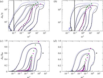
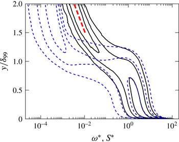
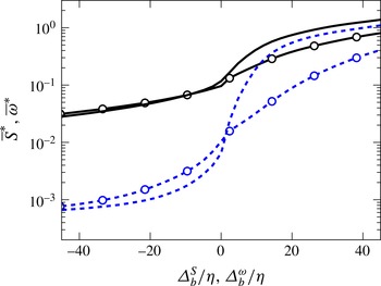
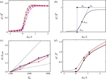
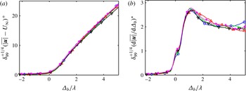
1 Introduction
It has been known since the early days of turbulence research that the near-wall region of boundary layers follows the law of the wall, but that the outer region is influenced by the interaction between turbulence and the free stream (Klebanoff Reference Klebanoff1955), whose most obvious manifestation is the ‘wake’ component of the mean velocity profile (Coles Reference Coles1956; Jiménez et al. Reference Jiménez, Hoyas, Simens and Mizuno2010). Early work by Corrsin (Reference Corrsin1943) revealed the presence of a sharp but irregular boundary between turbulent and non-turbulent flow, and the intermittent character of the flow near that boundary. It is also known that, although the outer part of boundary layers has some similarities to a wake (Coles Reference Coles1956), intermittency does not behave identically in different flows (Gartshore Reference Gartshore1966). This is true even if the extent of the intermittent region, quantified by Townsend (Reference Townsend1948) in terms of the fraction of time during which a given point is turbulent, is found to be similar in many flows.
Much of the research on the turbulent/non-turbulent (T/NT) interface has dealt with the entrainment process by which the irrotational flow acquires vorticity. An important early result was that the surface area of the T/NT interface is much larger than its projected area in the direction normal to the wall, and that it is intensely folded (Fiedler & Head Reference Fiedler and Head1966). This observation was the origin of two conjectures summarised by Townsend (Reference Townsend1976). The first one is that the interface itself has similar mass transfer per unit area in all turbulent flows, and that the different entrainment rates (stronger in jets and wakes, weaker in boundary layers and in plane mixing layers) are due to different folding intensities. The second conjecture has to do with the details of the entrainment mechanism. It is clear that irrotational fluid can only acquire vorticity by viscous diffusion (Corrsin & Kistler Reference Corrsin and Kistler1955). However, if the interface is sufficiently folded, large pockets of irrotational flow can be trapped by large coherent structures and driven deep into the turbulent region before acquiring vorticity. To add some nomenclature, small-scale entrainment is called nibbling, while the process by which large blobs of irrotational fluid are swallowed by the turbulent flow before becoming vortical is called engulfment (Mathew & Basu Reference Mathew and Basu2002). The ongoing discussion on the relative importance of the two entrainment mechanisms hinges in part on the understanding of the geometry of the T/NT interface.
It is challenging to capture this geometry in both experiments and simulations, partly because of its complexity. The thickness of the intermittent zone is comparable to the boundary-layer thickness,
 ${\it\delta}_{99}$
(Corrsin & Kistler Reference Corrsin and Kistler1955), while we will see that the strong gradients present in the interface contain some of the shortest scales in the flow. The interface inherits the fractal-like properties of the underlying turbulent flow (Sreenivasan, Ramshankar & Meneveau Reference Sreenivasan, Ramshankar and Meneveau1989), and, since turbulent flows typically contain eddies of all possible sizes between the smallest and largest scales, all of them have to be considered when the interface geometry is studied. As a result, important questions about entrainment in turbulent flows had to wait for the necessary data to be available.
Some experimental techniques are able to capture the interface with considerable detail, and the methods described in Prasad & Sreenivasan (Reference Prasad and Sreenivasan1989) are still used today. The properties of the flow surrounding the interface could not be measured until the advent of particle image velocimetry (Westerweel et al. Reference Westerweel, Hofmann, Fukushima and Hunt2002) and particle tracking velocimetry (Holzner et al. Reference Holzner, Liberzon, Nikitin, Lüthi, Kinzelbach and Tsinober2008). However, experiments are typically restricted to two-dimensional sections of the flow, and the three-dimensional description of the field requires direct numerical simulations (DNS).
Just like experiments, simulations have limitations. The range of available scales is the most obvious, and is crucial if the scaling properties of a phenomenon are to be studied. Direct numerical simulations at Reynolds numbers large enough to observe a reasonable scale separation are a recent achievement. While there have been boundary-layer simulations at moderate Reynolds numbers for some time (Jiménez et al. Reference Jiménez, Hoyas, Simens and Mizuno2010; Schlatter & Örlü Reference Schlatter and Örlü2010; Lee & Sung Reference Lee and Sung2013), a domain size sufficiently large to obtain a deep T/NT interface requires state-of-the-art DNS (Pirozzoli & Bernardini Reference Pirozzoli and Bernardini2013; Sillero, Jiménez & Moser Reference Sillero, Jiménez and Moser2013). The Reynolds numbers of these newer simulations are comparable to those of most experiments for which the interface has been analysed in any detail.
These larger and more accurate representations of the flow field, and better analysis tools, have called into question the consensus of what the dominant mechanism of entrainment is. Dahm & Dimotakis (Reference Dahm and Dimotakis1987), Ferre et al. (Reference Ferre, Mumford, Savill and Giralt1990), Mungal, Karasso & Lozano (Reference Mungal, Karasso and Lozano1991) and Dimotakis (Reference Dimotakis2000) suggested that engulfment is the dominant process, but later works like Mathew & Basu (Reference Mathew and Basu2002) and Westerweel et al. (Reference Westerweel, Fukushima, Pedersen and Hunt2005) emphasise again the importance of nibbling. The dichotomy may have something to do with the level of description desired, since it is clear that viscosity is the ultimate mechanism for vorticity diffusion, but it is equally clear that the complex geometry of the interface has to be taken into account in determining the rate of diffusion.
Determination of which scales are most relevant to entrainment requires the study of the turbulent structures in the vicinity of the interface, which implies the analysis of the properties of the flow in a reference frame linked to the interface itself. Fiedler & Head (Reference Fiedler and Head1966) presented results obtained from hot wires, but it was not until the work of Bisset, Hunt & Rogers (Reference Bisset, Hunt and Rogers2002), Westerweel et al. (Reference Westerweel, Hofmann, Fukushima and Hunt2002), da Silva, dos Reis & Pereira (Reference da Silva, dos Reis and Pereira2011) and van Reeuwijk & Holzner (Reference van Reeuwijk and Holzner2014) that conditional profiles relevant to the scaling of the interface were shown. Bisset et al. (Reference Bisset, Hunt and Rogers2002) mentioned that the T/NT interface could contain at least two layers with possibly different scaling properties: a turbulent region where the major exchanges between the irrotational fluid and the fully turbulent core occur, and a thinner viscous superlayer at its outer boundary, already conjectured by Corrsin & Kistler (Reference Corrsin and Kistler1955). A similar observation was made recently by Ishihara, Ogasawara & Hunt (Reference Ishihara, Ogasawara and Hunt2015) for a boundary layer. A recent review of the state of the art is given in da Silva et al. (Reference da Silva, Hunt, Eames and Westerweel2014a ).
The length scales of the interface provide information about the configuration of the nearby eddies, and about how they are affected by the irrotational flow. We define in this paper the T/NT interface as the region in which the properties of the flow are neither fully turbulent nor completely irrotational, and we are interested in describing how this transition is structured. Two important questions concern the thickness of the transition layer, and whether it can be further subdivided into distinct sublayers. The main candidates for the scaling of the T/NT interface are the Kolmogorov viscous length
 ${\it\eta}$
and the Taylor microscale
 ${\it\lambda}$
. The thickness of the vorticity interface of a DNS temporal jet was computed by da Silva & Taveira (Reference da Silva and Taveira2010) and found to be of the order of the Taylor microscale, and Gampert et al. (Reference Gampert, Narayanaswamy, Schaefer and Peters2013) were able to scale quite accurately with
 ${\it\lambda}$
the average thickness of the interface of a passive scalar in a jet over the Reynolds number range
 $Re_{{\it\lambda}}=61{-}141$
. This would agree with the theory described in Hunt & Durbin (Reference Hunt and Durbin1999) who, on the assumption that the interface is subject to a relatively strong local shear, noted that eddies would be blocked and squeezed instead of escaping to the irrotational side. Such an interface would have different dynamics from the rest of the flow and a characteristic thickness of
 $O({\it\lambda})$
.
The goal of this paper is to study the properties of the T/NT interface in a turbulent boundary layer, with emphasis on the relatively large-scale interactions across the fractal intermittent layer, rather than on the thinner viscous superlayer. We also analyse the consequences of the threshold used for interface detection. New methods are developed for the geometric characterisation of surfaces of arbitrary complexity in three-dimensional space, and for the conditional analysis of scalar fields with respect to those surfaces. These methods are used to describe the properties of the flow depending on its position relative to the T/NT interface, and to determine the characteristic thickness of the interface layer. The choice of the identification threshold is given special attention, as well as the choice of the variable being thresholded.
The paper is organised as follows. The next section is a short description of the data used in this research. The characteristics of the intermittent zone that are relevant to the detection of a T/NT interface based on a vorticity isocontour are presented in § 3, followed in § 4 by a quantitative analysis of the geometrical properties of the interface and its dependence on the threshold. Section 5 presents the conditional analysis of the flow using the interface as a reference frame. In particular, §§ 5.5 and 5.6 describe the structure of the vorticity and of other velocity gradients within the T/NT interface layer, and § 5.7 discusses the determination of its thickness. Finally, § 6 explores the behaviour of the velocity magnitude across the interface, and § 7 concludes.
2 Description of the data
The boundary layer is simulated in a rectangular box over a no-slip smooth wall. The spanwise boundary conditions are periodic, and inflow and outflow conditions are imposed in the streamwise direction. A transpiration velocity in the boundary opposite to the wall keeps the pressure gradient very close to zero. The simulation code and its implementation are thoroughly explained in Simens et al. (Reference Simens, Jiménez, Hoyas and Mizuno2009), and the modifications to achieve higher Reynolds numbers are presented in Borrell, Sillero & Jiménez (Reference Borrell, Sillero and Jiménez2013). The axes in the streamwise, wall-normal and spanwise directions are
 $x$
,
 $y$
and
 $z$
respectively. The total velocity vector is
 $\boldsymbol{u}$
, with components along each axis
 $u$
,
 $v$
and
 $w$
respectively. Wall units are defined in terms of the friction velocity
 $u_{{\it\tau}}$
and of the kinematic viscosity
 ${\it\nu}$
, and are denoted by a ‘
 $+$
’ superscript. The brackets
 $\langle \cdot \rangle$
denote the ensemble average at a given wall-normal location, and primes denote root-mean-squared values. Both are functions of
 $x$
and
 $y$
, and are obtained from field snapshots sufficiently separated in time (approximately 0.2 flow turnovers) to discard spurious correlations between the samples. The boundary-layer thickness is
 ${\it\delta}_{99}$
, defined as the distance to the wall at which
 $\langle u\rangle$
is 99 % of the free-stream velocity. The Kolmogorov length is
 ${\it\eta}=({\it\nu}^{3}/\langle {\it\varepsilon}\rangle )^{1/4}$
, where
 $$\begin{eqnarray}\langle {\it\varepsilon}\rangle ={\it\nu}[\langle |\boldsymbol{{\rm\nabla}}(\boldsymbol{u}-\langle \boldsymbol{u}\rangle )|^{2}\rangle ]\end{eqnarray}$$
is the turbulent kinetic-energy pseudo-dissipation rate. A third relevant length is the Taylor microscale
 $$\begin{eqnarray}{\it\lambda}=\sqrt{\frac{15{\it\nu}u^{\prime 2}}{\langle {\it\varepsilon}\rangle }},\end{eqnarray}$$
where
 $u^{\prime 2}=[\langle |\boldsymbol{u}|^{2}\rangle -|\langle \boldsymbol{u}\rangle |^{2}]/3$
is the one-component velocity fluctuation intensity computed under the assumption of isotropy. Table 1 and figure 1 summarise the important parameters and characteristics of the simulation, which was designed to achieve convergence of all of the scales of the flow in the domain labelled
 $BL$
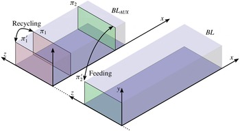
, over a range of Reynolds numbers as wide as possible. Two simulations are run simultaneously with a synchronised time step, but the purpose of the auxiliary simulation
 $BL_{AUX}$
is just to provide inflow boundary conditions for
 $BL$
. Only data from
 $BL$
are used in this paper. A detailed discussion of the effects of the inflow and of the evolution with
 $x$
of the flow properties towards their asymptotic behaviour can be found in Sillero et al. (Reference Sillero, Jiménez and Moser2013).
Sketch of the simulation and the boundary conditions. The inflow boundary conditions for
 $BL$
are obtained from
 $BL_{AUX}$
, copying the plane
 ${\it\pi}_{2}$
to the first plane of
 $BL$
at
 ${\it\pi}_{2}^{\prime }$
. The streamwise location of
 ${\it\pi}_{2}$
is chosen so that the flow has recovered from the recycling scheme (
 ${\it\pi}_{1}$
is recycled to
 ${\it\pi}_{1}^{\prime }$
) used to start
 $BL_{AUX}$
from a turbulent inflow condition.

Summary of important parameters of the simulation. Here,
 $N_{x}$
,
 $N_{y}$
and
 $N_{z}$
are the size of the computational grid. The Taylor-microscale Reynolds number
 $Re_{{\it\lambda}}$
, the Kolmogorov length
 ${\it\eta}$
and the Taylor microscale
 ${\it\lambda}$
are estimated at
 $y=0.6{\it\delta}_{99}$
. The running time
 $T$
is normalised with properties at the middle of the
 $BL$
box.

Because both
 ${\it\lambda}$
and
 ${\it\eta}$
depend on the distance to the wall, especially in the intermittent region, the values used below to normalise lengths are taken at
 $y=0.6{\it\delta}_{99}$
. This is the point farthest from the wall that can be assumed to be roughly free of intermittency corrections. We will see below that the dissipation decays in the turbulent parts of the layer approximately as in non-intermittent internal turbulent flows (see figure 3
a), so that
 ${\it\lambda}\propto y^{1/2}$
and
 ${\it\eta}\propto y^{1/4}$
(Tennekes & Lumley Reference Tennekes and Lumley1972). As a consequence, the reference values used below are proportional to ‘notional’ values at the edge of the layer,
 ${\it\eta}(0.6{\it\delta}_{99})/{\it\eta}({\it\delta}_{99})\approx 0.6^{1/4}=0.88$
and
 ${\it\lambda}(0.6{\it\delta}_{99})/{\it\lambda}({\it\delta}_{99})\approx 0.77$
, and the scaling properties with respect to the mid-layer values are the same as those with respect to the boundary-layer edge.
The simulation agrees excellently with previous experiments and DNS (Sillero et al.
Reference Sillero, Jiménez and Moser2013; Sillero, Jiménez & Moser Reference Sillero, Jiménez and Moser2014). The Taylor-microscale Reynolds number,
 $Re_{{\it\lambda}}={\it\lambda}u^{\prime }/{\it\nu}\simeq O(100)$
, is comparable to those of most experiments and simulations used in the analysis of the T/NT interface in free shear flows, and higher than those in the boundary layers previously used for that purpose. The microscale Reynolds numbers in table 1 are evaluated at
 $y=0.6{\it\delta}_{99}$
, but they vary little in the range
 $y/{\it\delta}_{99}=0.3$
–
 $0.6$
and only start to decrease where the flow intermittency becomes important. They can be taken as representative of the ‘turbulent’
 $Re_{{\it\lambda}}$
near the T/NT interface. The friction Reynolds number
 ${\it\delta}_{99}^{+}$
ranges over a factor of two (see table 1), allowing it to be used as a parameter in the analysis. The resulting ratio of
 ${\it\delta}_{99}/{\it\eta}$
ranges over a factor of 1.8, easily allowing the distinction between outer
 $({\it\delta}_{99})$
and viscous
 $({\it\eta})$
scaling. The corresponding range of
 ${\it\lambda}/{\it\eta}$
is only approximately 1.2, but is still sufficient to distinguish between scalings with the two quantities. The averaged properties of the data set have been accumulated over the complete history of the simulation after discarding the initial transient. Some of the more detailed results have been obtained from at least eight flow snapshots, sufficiently separated to ensure statistical independence.
3 The interface detection criterion
The first step to study the T/NT interface is to define the criterion that discriminates between turbulent and non-turbulent flow. Unfortunately, different methods produce different interfaces, and the criteria found in the literature are variable enough to be difficult to compare consistently. Historically, the first interface detections were based on a cutoff frequency for the one-point streamwise-velocity signal, in the expectation that turbulent fluctuations could be easily distinguished by their faster time scales. As better descriptions of the flow became available, the interface came to be defined by an indicator function with two components: a scalar field related to the turbulent fluctuations, and a threshold. Prasad & Sreenivasan (Reference Prasad and Sreenivasan1989) use the concentration of a passive scalar injected in the turbulent side, and threshold it at the least probable value of the concentration. da Silva et al. (Reference da Silva, dos Reis and Pereira2011), in jets, and Bisset et al. (Reference Bisset, Hunt and Rogers2002), in wakes, use the vorticity magnitude as indicator, and a particularly low vorticity value as the threshold. In boundary layers, Jiménez et al. (Reference Jiménez, Hoyas, Simens and Mizuno2010) also use the vorticity magnitude, and a threshold based on a sharp jump in its probability density function (PDF) at
 $y={\it\delta}_{99}$
. Chauhan et al. (Reference Chauhan, Philip, de Silva, Hutchins and Marusic2014) use a measure of the kinetic-energy fluctuations as their scalar, and choose the highest threshold for which the PDF of the height of the interface above the wall can be fitted by a Gaussian.
Our criterion is based on the magnitude of the total vorticity,
 ${\it\omega}=|{\bf\omega}|=|\boldsymbol{{\rm\nabla}}\wedge \boldsymbol{u}|$
, which has several desirable properties as a turbulence indicator and can easily be obtained from DNS. In the first place, the incompressible identity
 ${\rm\nabla}^{2}\boldsymbol{u}=-\boldsymbol{{\rm\nabla}}\wedge {\bf\omega}$
implies that the characteristic turbulent dissipation of energy requires vorticity. Second, while velocity gradients can be created by pressure fluctuations in potential flow, there is no inviscid mechanism to create vorticity fluctuations. As a consequence, even if vorticity is not conserved, any vorticity in the boundary layer is ultimately linked to the wall. It should be noted that some of these desirable properties of the vorticity magnitude do not extend to its individual components. For example, there can be energy dissipation in the absence of one vorticity component, and any component can easily appear or disappear by simple rotation. More significantly, although vorticity is very approximately isotropic away from the wall (Jiménez Reference Jiménez2013), the solenoidality of the curl requires that the vorticity vector should be roughly parallel to any surface across which its magnitude drops or increases sharply. The geometry of the vorticity magnitude and of any one of its component cannot be assumed to be similar.
We thus define a point as turbulent if
 $$\begin{eqnarray}{\it\omega}(x,y,z,t)>{\it\omega}_{0},\end{eqnarray}$$
and the T/NT interface by
 ${\it\omega}={\it\omega}_{0}$
, and turn our attention to determining the threshold
 ${\it\omega}_{0}$
, either from the properties of the resulting interface or from comparisons with previous investigations.
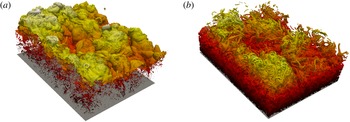
The simplest tool is three-dimensional visualisation, preferably of a relatively large part of the interface. Figure 2(a,b) shows the interface in a domain whose wall-parallel size is several boundary-layer thicknesses, for two thresholds separated by an order of magnitude. The two panels are different. Figure 2(a) can be described as a moderately complex envelope with scattered small regions of low vorticity within the turbulent side, while figure 2(b) has a large number of handles and contortions which span a significant fraction of the boundary-layer thickness.
Vorticity magnitude isosurfaces of the same region of the present data at
 ${\it\delta}_{99}^{+}\simeq 2000$
, of size
 $3{\it\delta}_{99}\times 2{\it\delta}_{99}$
in the streamwise and spanwise directions respectively: (a)
 ${\it\omega}_{0}^{+}=5\times 10^{-4}$
(
 ${\it\omega}_{0}^{\ast }=0.022$
), (b)
 ${\it\omega}_{0}^{+}=5\times 10^{-3}$
(
 ${\it\omega}_{0}^{\ast }=0.22$
). For the definition of
 ${\it\omega}^{\ast }$
, see (3.4). The flow is from top left to bottom right, but note that the spanwise and streamwise directions are barely distinguishable.

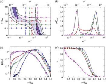
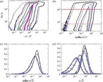
Another useful tool is the joint PDF of the vorticity magnitude and of the vertical distance to the wall, which is presented in figure 3(a) as a premultiplied PDF,
 ${\it\omega}{\it\Gamma}_{{\it\omega},y}$
, to account for the logarithmic scale of the vorticity. It has two well-defined regions. The high-vorticity near-wall points of the turbulent core of the boundary layer are in the lower right-hand corner. Points far from the wall with very low vorticity, representing the ideally irrotational non-turbulent free stream, are in the top-left corner. Their residual vorticity is due to the finite accuracy of the inflow condition, but it is approximately four orders of magnitude weaker than the turbulent values, and easily distinguished from them. In the present data set, the details of the joint PDF depend only weakly on the Reynolds number.
The quantity
 ${\it\omega}{\it\Gamma}_{{\it\omega},y}$
was also obtained by da Silva, Taveira & Borrell (Reference da Silva, Taveira and Borrell2014b
) for other external turbulent flows, showing that the intermittent region is comparable in all the tested cases. There is always a sharp jump in vorticity, and a relatively wide range of choices for the threshold.
(a) Premultiplied joint PDF,
 ${\it\omega}{\it\Gamma}_{{\it\omega},y}$
, of the wall-normal distance and the vorticity magnitude. The contours contain 50 %, 90 % and 99 % of points. Two vorticity scales are provided, wall units
 ${\it\omega}^{+}$
, and the
 ${\it\omega}^{\ast }$
defined in (3.4). The line with open circles is
 ${\it\omega}^{+}=(y^{+})^{-1/2}$
. The horizontal and vertical lines correspond to the one-dimensional sections in (b,c), using the same markers. (b) Sections of
 ${\it\omega}{\it\Gamma}_{{\it\omega},y}$
at four different distances to the wall: ♢,
 $y/{\it\delta}_{99}=0.5$
; ▵, 0.75; ▿, 1; ▫, 1.25. (c) One-dimensional PDF,
 $Q(y_{I})$
, of the vertical position of the interface when its average position is ♢,
 $\langle y_{I}\rangle /{\it\delta}_{99}=1$
 $({\it\omega}_{0}^{\ast }=0.022)$
; ▵, 0.9
 $({\it\omega}_{0}^{\ast }=0.09)$
; ▿, 0.8
 $({\it\omega}_{0}^{\ast }=0.2)$
; ▫,
 ${\it\omega}_{0}^{\ast }=2.0$
. The vorticity thresholds of the first and third curves are those of the isosurfaces in figures 2(a) and 2(b) respectively. The dashed line fitting each curve is the Gaussian distribution with the same mean and standard deviation. (d) Intermittency factor for the four thresholds in (c). In all cases,
 ${\it\delta}_{99}^{+}\simeq 1500$
.

On the turbulent side of the PDF, the mode of the vorticity distribution follows closely the expected
 $y$
-dependence of its root-mean-squared value,
 ${\it\omega}^{\prime }$
, which can be estimated from the approximate balance between the production and the pseudo-dissipation of the turbulent kinetic energy,
 $$\begin{eqnarray}{\it\nu}{\it\omega}^{\prime 2}\simeq -\langle uv\rangle \frac{\partial \langle u\rangle }{\partial y}\simeq \frac{u_{{\it\tau}}^{3}}{{\it\kappa}y},\end{eqnarray}$$
where
 ${\it\kappa}\simeq 0.4$
is the von Kármán constant. Equation (3.2) holds above
 $y^{+}\simeq 50$
(Jiménez Reference Jiménez2013), and provides a characteristic magnitude for the vorticity fluctuations,
 $$\begin{eqnarray}\langle {\it\omega}^{+}\rangle \simeq ({\it\kappa}y^{+})^{-1/2}.\end{eqnarray}$$
We will use this dependence, particularised at the edge of the boundary layer, to define dimensionless star units for the vorticity,
 $$\begin{eqnarray}{\it\omega}^{\ast }={\it\omega}({\it\delta}_{99}^{+})^{1/2}({\it\nu}/u_{{\it\tau}}^{2}),\end{eqnarray}$$
which are linked to the interface. The usual scaling
 ${\it\omega}^{+}={\it\omega}{\it\nu}/u_{{\it\tau}}^{2}$
is linked to the wall. The ratio
 ${\it\omega}^{\ast }/{\it\omega}^{+}$
varies by a factor of 1.4 in our range of Reynolds numbers, and we will see below that star units collapse most properties of the interface substantially better than wall units.
The definition of
 ${\it\omega}^{\ast }$
can be adapted to flows other than the boundary layer by normalising the vorticity with the root-mean-squared value of the enstrophy fluctuations of the turbulent fluid close to the interface. We will occasionally do this for the purpose of comparison.
There is a band connecting the turbulent and non-turbulent regions of figure 3(a) which spans several orders of magnitude of the vorticity and extends over
 $y/{\it\delta}_{99}=0.3{-}1.5$
. Four sections of the premultiplied PDF at different
 $y$
are presented in figure 3(b). The one at
 $y={\it\delta}_{99}$
is particularly interesting, because it shows the separation between the two regions of the flow. Its two mild peaks bracket a plateau three orders of magnitude wide, from the expected turbulent value
 ${\it\omega}^{\ast }\simeq {\it\kappa}^{-1/2}=1.6$
on the right to the free-stream residual vorticity on the left. Any vorticity within this plateau could, in principle, be used as a threshold for the interface, but, even with generous safety margins at both ends, this leaves a full order of magnitude of possible choices. This would not be a problem if thresholds within this range produced similar results, but they do not. The two isosurfaces in figure 2 are obtained with thresholds within the plateau. They correspond to the first and third leftmost vertical lines in figure 3(a).
Other quantities frequently used to analyse the properties of the edge of boundary layers can be obtained from
 ${\it\Gamma}_{{\it\omega},y}$
. The intermittency parameter
 $$\begin{eqnarray}{\it\gamma}(y;{\it\omega}_{0})=\left.\int _{{\it\omega}_{0}}^{\infty }{\it\Gamma}_{{\it\omega},y}\,\text{d}{\it\omega}\right/\int _{0}^{\infty }{\it\Gamma}_{{\it\omega},y}\,\text{d}{\it\omega}\end{eqnarray}$$
is the probability that a point at a given distance from the wall is turbulent according to (3.1). The sections of
 ${\it\Gamma}_{{\it\omega},y}$
at constant
 ${\it\omega}$
provide the marginal probability distribution of the distance,
 $y_{I}$
, to the wall of the interface defined as a vorticity isocontour,
 $$\begin{eqnarray}Q(y_{I};{\it\omega}_{0})=-\partial {\it\gamma}/\partial {\it\omega}_{0}={\it\Gamma}_{{\it\omega}_{0},y}\left/\int _{0}^{\infty }{\it\Gamma}_{{\it\omega}_{0},y}\,\text{d}y.\right.\end{eqnarray}$$
It should be noted that, because of several approximations analysed in detail below, the effective definition of the interface does not usually exactly coincide with this vorticity isosurface. Four examples of
 $Q(y_{I})$
and
 ${\it\gamma}(y)$
are presented in figure 3(c,d). The thresholds of the first three are chosen so that the average height of the T/NT interface is
 $\langle y_{I}\rangle /{\it\delta}_{99}=1$
, 0.9 and 0.8 respectively, and are within the plateau in figure 3(a). The first and third ones are used in figure 2. This confirms that the threshold has an important effect on the geometry of the T/NT interface, even for properties that are easily measurable. It should be noted that, although
 $Q(y_{I})$
and
 ${\it\gamma}(y)$
are linked by the first equality in (3.6),
 ${\it\gamma}$
is not very sensitive to the changes in
 $Q$
, and always tends to look approximately Gaussian. The fourth line in figure 3(c,d), marked with open squares, is
 ${\it\omega}_{0}^{\ast }=1.6$
and corresponds to the rightmost end of the plateau in figure 3(a). It behaves differently from the other three PDFs, and neither
 $Q(y_{I})$
nor
 ${\it\gamma}(y)$
can be approximated as Gaussian. This threshold does not represent the interface any more, and can best be understood as describing the internal structure of the turbulent vorticity.
The mean,
 $\langle y_{I}\rangle$
, and standard deviation,
 ${\it\sigma}(y_{I})$
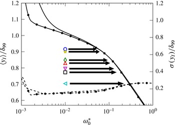
, of the interface height are presented in figure 4 as functions of
 ${\it\omega}_{0}$
. Three regimes can be distinguished. The first one, below
 ${\it\omega}_{0}^{\ast }=2\times 10^{-3}$
, reflects the vorticity fluctuations in the free stream, and therefore is basically a numerical artefact. In the second one, between
 ${\it\omega}_{0}^{\ast }=2\times 10^{-3}$
and
 ${\it\omega}_{0}^{\ast }=0.1$
, the average position of the interface is
 $\langle y_{I}\rangle \simeq {\it\delta}_{99}$
, and
 $Q(y_{I})$
is well approximated by a normal distribution with symmetric tails (figure 3
c). Above
 ${\it\omega}_{0}^{\ast }=0.1$
, the left tail of
 $Q(y_{I})$
begins to penetrate the turbulent core,
 $\langle y_{I}\rangle$
drops faster with the threshold, and the standard deviation increases slightly. It should be noted that figure 4 includes the two extreme Reynolds numbers in our simulation, which agree well except for thresholds low enough to represent the free stream. This good collapse with the Reynolds number suggests that the extent of the intermittent region is not expected to change significantly with increasing
 ${\it\delta}_{99}^{+}$
.
The solid lines and left vertical axis are the average,
 $\langle y_{I}\rangle$
, of the height of the vorticity isosurface, and the dashed lines and right vertical axis are its standard deviation, both as functions of
 ${\it\omega}_{0}^{\ast }$
. The values of
 $\langle y_{I}\rangle$
in table 2 are marked by their corresponding symbols, with an arrow pointing to the matching
 ${\it\omega}_{0}^{\ast }$
. Lines without symbols are
 ${\it\delta}_{99}^{+}=1100$
; those with symbols are
 ${\it\delta}_{99}^{+}=1900$
.

Properties of
 $Q(y_{I})$
for the different values of
 $\langle y_{I}\rangle$
found in the literature. The standard deviation
 ${\it\sigma}(y_{I})$
and the threshold
 ${\it\omega}_{0}^{\ast }$
are obtained from the present data set, and correspond to the threshold required to match
 $\langle y_{I}\rangle$
for each entry.
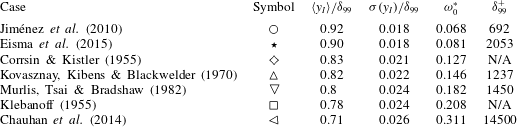
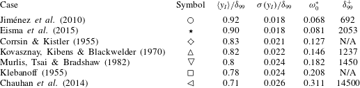
The values of
 $\langle y_{I}\rangle$
available in the literature are compiled in table 2 and marked with their corresponding symbols in figure 4. They can be used as guides in choosing our threshold. It should be noted that there is a fairly large spread between the choices of Jiménez et al. (Reference Jiménez, Hoyas, Simens and Mizuno2010) and of Chauhan et al. (Reference Chauhan, Philip, de Silva, Hutchins and Marusic2014), which, if translated to vorticity thresholds using figure 4, would imply half an order of magnitude in
 ${\it\omega}_{0}^{\ast }$
. The thresholds in figures 2(a) and 2(b) correspond to
 $\langle y_{I}\rangle \approx {\it\delta}_{99}$
and
 $0.8{\it\delta}_{99}$
respectively.
Figure 3(b) suggests that
 ${\it\omega}_{0}^{\ast }=0.022$
, for which
 $\langle y_{I}\rangle ={\it\delta}_{99}$
, should be a reasonable threshold, since it is at this height that the vorticity PDF is widest and bimodal. However, figure 4 and table 2 show that this threshold is an order of magnitude lower than most values used in previous works.
The definition in Prasad & Sreenivasan (Reference Prasad and Sreenivasan1989) can be adapted to cases without a passive scalar, using the vorticity magnitude as a tracer (Gampert et al.
Reference Gampert, Boschung, Hennig, Gauding and Peters2014; da Silva et al.
Reference da Silva, Taveira and Borrell2014b
). Applying this criterion to the present data would imply
 ${\it\omega}_{0}^{\ast }=0.05$
and
 $\langle y_{I}\rangle =0.95{\it\delta}_{99}$
, which is comparable to figure 2(a), and again lower than the values found in the literature. On the other hand, da Silva et al. (Reference da Silva, Taveira and Borrell2014b
) found that
 ${\it\omega}^{\ast }=0.01$
, corresponding to roughly
 ${\it\omega}/{\it\omega}^{\prime }=0.1$
, is a reasonable choice in jets and shear-free turbulence, and it can be shown that there is very little difference in our case between this choice and the value
 ${\it\omega}^{\ast }=0.022$
suggested above. da Silva et al. (Reference da Silva, Taveira and Borrell2014b
) also include a proof that this definition is related to the one used by Watanabe et al. (Reference Watanabe, Sakai, Nagata, Ito and Hayase2015) to detect their irrotational boundary.
If we try to apply the criterion of Chauhan et al. (Reference Chauhan, Philip, de Silva, Hutchins and Marusic2014) to the vorticity field, we find that
 $Q(y_{I})$
is approximately Gaussian for
 ${\it\omega}_{0}^{\ast }\in (2\times 10^{-3}{-}0.1)$
. This corresponds to
 $\langle y_{I}\rangle /{\it\delta}_{99}\in (1.1{-}0.9)$
. Although the lowest end of this range agrees with the mean interface height in Jiménez et al. (Reference Jiménez, Hoyas, Simens and Mizuno2010), it is very far from the value
 $\langle y_{I}\rangle /{\it\delta}_{99}=0.71$
obtained by Chauhan et al. (Reference Chauhan, Philip, de Silva, Hutchins and Marusic2014). This shows that the vorticity and velocity interfaces are different, and that the criterion in Chauhan et al. (Reference Chauhan, Philip, de Silva, Hutchins and Marusic2014) should not be used for the vorticity.
In summary, since neither the intermittency properties of the interface nor previous studies provide guidance on a unique vorticity threshold, we defer our decision until we study the evolution of the interface over the rather wide range
 ${\it\omega}_{0}^{\ast }\in (0.001{-}10)$
.
4 The geometry of the T/NT interface
In this section we study the geometry of the T/NT interface defined as an isosurface separating vortical from irrotational fluid. As such, we can use its dependence on
 ${\it\omega}_{0}$
to explore the geometry of the two flow regimes as the isosurface moves from one to the other. This will also help us to decide which threshold is best suited for each particular purpose. For example, figure 2(a) appears to represent the free stream better, while figure 2(b) is more representative of the interior of turbulence.
4.1 Bubbles and drops
The first step is to define the interface separating the flow into turbulent and non-turbulent regions. This is not as straightforward as the previous section may suggest. Figure 2(b) shows that the vorticity isocontour is not usually a singly connected surface. Depending on the threshold, there may be a few or several thousands of disconnected components of the isosurface, but one of them is typically much larger than the rest and divides the computational box into two large disjoint regions. The remaining isosurface components can be classified as envelopes of low-vorticity bubbles within the turbulent region (figure 5 c), or of high-vorticity drops in the free stream. It will be shown in § 5 that, although there can be a large number of bubbles, they are usually too small to contribute significantly to most quantities related to the T/NT interface. There are generally very few drops. In consequence, the rest of this paper defines the interface as the largest singly connected component of the vorticity isosurface that separates ‘smoothed’ irrotational and vortical regions from which drops and bubbles have been eliminated.
Sketch of the three basic geometrical features in the vorticity isosurface: (a) handles, (b) pockets and (c) bubbles.

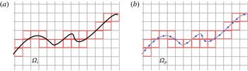
The algorithm to obtain this largest component is sketched in figure 6. We first decompose the computational domain into computational cells (voxels). The flow properties are defined at their vertices. We next obtain the set
 ${\it\Omega}_{{\it\omega}>}$
of voxels for which at least one vertex has a vorticity higher than the threshold (figure 6
a). This set contains the drops and the bulk of the turbulent flow. Similarly, we obtain the set
 ${\it\Omega}_{{\it\omega}<}$
for which at least one vertex has a vorticity lower than the threshold, containing the bubbles and the bulk of non-turbulent flow (figure 6
b). Each of these sets has a connected component many times larger than the rest (approximately seven orders of magnitude in our case). In the case of
 ${\it\Omega}_{{\it\omega}>}$
, this set represents the bulk of the turbulent flow,
 ${\it\Omega}_{t}$
, while in the case of
 ${\it\Omega}_{{\it\omega}<}$
it represents the bulk of the free stream,
 ${\it\Omega}_{n}$
. The sets of voxels containing the drops,
 ${\it\Omega}_{d}$
, and the bubbles,
 ${\it\Omega}_{b}$
, are obtained by subtracting these largest components from their respective sets. Thus,
 ${\it\Omega}_{d}={\it\Omega}_{{\it\omega}>}-{\it\Omega}_{t}$
and
 ${\it\Omega}_{b}={\it\Omega}_{{\it\omega}<}-{\it\Omega}_{n}$
. The final step is to define the set of voxels of the cleaned T/NT interface as (figure 6
c)
 $$\begin{eqnarray}{\it\Omega}_{i}=\underbrace{({\it\Omega}_{t}\cup {\it\Omega}_{b})}_{\text{Turbulent side}}\cap \underbrace{({\it\Omega}_{n}\cup {\it\Omega}_{d})}_{\text{Non\text{-}turbulent side}}.\end{eqnarray}$$
It should be noted that the two terms of this equation are effective definitions of the smoothed turbulent region (the bulk of the turbulent flow plus the bubbles) and the smoothed non-turbulent region (the bulk of the non-turbulent flow plus the drops).
(a) The set
 ${\it\Omega}_{{\it\omega}>}$
of voxels in which at least one vertex is
 ${\it\omega}>{\it\omega}_{0}$
. (b) The set
 ${\it\Omega}_{{\it\omega}<}$
of voxels where
 ${\it\omega}<{\it\omega}_{0}$
. (c) The set
 ${\it\Omega}_{i}$
of voxels that contain the interface, from (4.1).

Drops and bubbles should not be confused with other complications of the interface, such as the handles and overhangs or ‘pockets’ represented in figure 5(a,b). The former complicate the topology of the flow and cannot be eliminated. The latter are topologically neutral, but may be important from the experimental or dynamical point of view. They hide part of the surface to some observational procedures, and may be precursors of large-scale engulfing. At this point, the interface is still a set of voxels that has to be converted into a surface, but this representation is sufficient for the analysis in the next two sections.
4.2 Fractal dimension
Mandelbrot (Reference Mandelbrot1975) was the first to suggest that the hierarchy of turbulent eddies can be approximated by a fractal when the Reynolds number is large enough. This was first verified by Sreenivasan & Meneveau (Reference Sreenivasan and Meneveau1986) for the bulk of the flow, and by Sreenivasan et al. (Reference Sreenivasan, Ramshankar and Meneveau1989) for the T/NT interface. The latter also proposed a simple theory to relate the two results. The fractal dimension of the vorticity isosurface measures how contorted it is, and is a useful statistical measure of its complexity. The most widely used definition is the box-counting Kolmogorov capacity: if
 $N_{b}$
is the number of boxes of size
 $r$
required to cover a set
 ${\it\Omega}$
, such as the interface, the fractal dimension
 $D$
is defined by
 $N_{b}\propto r^{D}$
.
In practice, the computation of fractal dimensions is complicated because turbulence is only self-similar in a limited range of scales. Vorticity is smooth at scales of the order of the Kolmogorov microscale, and the largest eddies responsible for the energy input are not self-similar. In cases in which an extended power law is not immediately obvious, a reasonable redefinition of the box-counting dimension is
 $$\begin{eqnarray}\dim _{b}=-\lim _{r\rightarrow {\it\varsigma}}\frac{\log N_{b}}{\log r},\end{eqnarray}$$
where
 ${\it\varsigma}$
stands for the smallest possible box size at which the data set remains self-similar, or, in the present case, for the size of the computational voxels. This requirement is difficult to define, and it is hard to speak of a fractal unless the self-similar range extends over a reasonably wide range.
Sreenivasan et al. (Reference Sreenivasan, Ramshankar and Meneveau1989) found a clear power law from two-dimensional sections of the interface, and measured a constant dimension
 $D$
away from the saturation caused by the shortest and longest scales. They concluded that the interface is a monofractal in that range. Moisy & Jiménez (Reference Moisy and Jiménez2004) computed the fractal dimension of three-dimensional enstrophy isosurfaces in homogeneous turbulence, using the full three-dimensional field instead of cross-sections, and three-dimensional boxes instead of two-dimensional ones. They found that the self-similar range observed by Sreenivasan et al. (Reference Sreenivasan, Ramshankar and Meneveau1989) is only an approximation, and defined a local dimensional exponent to account for the dependence on the box size,
 $$\begin{eqnarray}D_{b}(r)=-\frac{\text{d}\log N_{b}}{\text{d}\log r}.\end{eqnarray}$$
This definition includes the previous two. If
 $D_{b}(r)$
is constant and the T/NT interface is a monofractal,
 $\dim _{b}=D=D_{b}(r)$
.
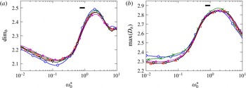
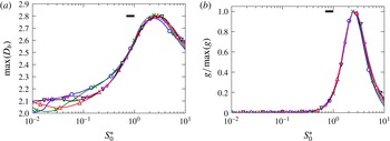
The local exponent (4.3) of our ‘cleaned’ interface is presented in figure 7 as a function of
 ${\it\omega}_{0}^{\ast }$
for several Reynolds numbers. Figure 7(a) plots
 $D_{b}$
for the smallest possible value of
 $r$
, and tries to approximate (4.2). Figure 7(b) plots the maximum value
 $D_{b}$
over the whole range of
 $r$
. The differences between the two figures quantify how far from a monofractal the T/NT interface is. The good collapse of the different Reynolds numbers when parametrised with
 ${\it\omega}_{0}^{\ast }$
should be noted. The black horizontal bar near the peaks of both figures is the variation of
 ${\it\omega}^{\ast }/{\it\omega}^{+}$
in our range of Reynolds number. A similar bar is included in all later figures that make a Reynolds number comparison, and measures how much the collapse of the different curves would deteriorate if the data had been normalised with
 ${\it\omega}_{0}^{+}$
instead of with
 ${\it\omega}_{0}^{\ast }$
.
Estimation of the box-counting fractal dimension, obtained in (a) from the local fractal exponent in the limit of small box size, and in (b) from the maximum of the local exponent over
 $r$
. The symbols represent different values of
 ${\it\delta}_{99}^{+}$
: ○, 1100;
 $\times$
, 1300; ▿, 1500; ▵, 1700;
 $\star$
, 1900. The horizontal bar is the variation of
 ${\it\omega}^{\ast }/{\it\omega}^{+}$
in our range of
 ${\it\delta}_{99}^{+}$
.

The dependence of
 $D_{b}$
on
 ${\it\omega}_{0}^{\ast }$
confirms the visual impression from figure 2 that the threshold has a dramatic effect on the interface. At low thresholds, the dimension approaches the smooth limit
 $D=2$
, but, at higher ones, the T/NT interface is significantly more convoluted. Sreenivasan et al. (Reference Sreenivasan, Ramshankar and Meneveau1989) predicted
 $D=7/3$
for the T/NT interface, precisely the value observed by de Silva et al. (Reference de Silva, Philip, Chauhan, Meneveau and Marusic2013) in a more recent experiment, which is within the range of the present results. It would correspond to
 ${\it\omega}_{0}^{\ast }\simeq 1$
in figure 7(a), and to the lowest possible dimension in figure 7(b).
Regardless of the differences in their absolute values, the two estimations of the fractal dimension in figure 7 behave similarly with respect to
 ${\it\omega}_{0}^{\ast }$
. There is a transition between
 ${\it\omega}_{0}^{\ast }\simeq 0.2$
and
 ${\it\omega}_{0}^{\ast }\simeq 2$
, across which the geometrical complexity of the interface increases significantly. This suggests that across this range the isosurface moves inside the turbulent core, where it reflects the geometrical features of the turbulent vorticity itself. It also follows from figure 4 that
 ${\it\omega}_{0}^{\ast }\simeq 0.2$
corresponds to the threshold for which the average location of the interface
 $\langle y_{I}\rangle$
decreases fastest as the threshold increases.
The decrease of the dimension beyond
 ${\it\omega}_{0}^{\ast }\simeq 2$
was already observed by Moisy & Jiménez (Reference Moisy and Jiménez2004), who used thresholds equivalent to
 ${\it\omega}_{0}^{\ast }\simeq 2{-}12$
to study the geometry of the volume of the vorticity in isotropic turbulence. There is no simple relation between the fractal dimensions of a set and of its surface, but Moisy & Jiménez (Reference Moisy and Jiménez2004) noted that in the limit of very high thresholds the vorticity would be reduced to a discrete cloud of points for which
 $D\simeq 0$
. A similar argument can be applied to the interface.
4.3 Genus
The geometric complexity of an object can also be characterised by its topological properties. The genus
 $g$
is a topological invariant of any connected orientable surface, and measures the number of its ‘handles’ (figure 5
a). A sphere has genus zero, a torus has genus one, and two connected tori have genus two. To the best of our knowledge, the genus was first used to characterise turbulent structures in homogeneous turbulence by Leung, Swaminathan & Davidson (Reference Leung, Swaminathan and Davidson2012), who cite instances of its earlier use in disciplines such as astrophysics. In most of those cases, the genus is obtained by integrating the mean and Gaussian curvatures over the interface, which requires a careful triangulation of the surface. This step is time consuming and prone to errors, and we bypass it by computing the genus directly from the Euler characteristic
 ${\it\chi}$
of the numerically defined contour. The algorithm is described in Lozano-Durán & Borrell (Reference Lozano-Durán and Borrell2016), and is optimised to exploit discrete data in structured grids.
Briefly, any numerical isosurface in a Cartesian grid is a polyhedron of stacked parallelepipeds. If
 $V$
is the number of vertices,
 $E$
is the number of edges and
 $F$
is the number of faces, its Euler characteristic is given by the Euler–Poincaré formula,
 $$\begin{eqnarray}{\it\chi}=V-E+F,\end{eqnarray}$$
and the genus is
 $$\begin{eqnarray}g=1-\frac{{\it\chi}}{2}.\end{eqnarray}$$
The genus is a measure of complexity, like the fractal dimension, but the two are not equivalent. A wrinkled piece of paper has genus zero, independently of the amount of wrinkling. A regular Brownian surface is defined as a fractal single-valued map on the real plane. Its fractal dimension is
 $D=2.5$
, but it has no handles (Russ Reference Russ1994).
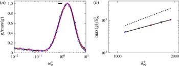
(a) Genus normalised with its maximum over
 ${\it\omega}_{0}$
. The horizontal bar is the variation of
 ${\it\omega}^{\ast }/{\it\omega}^{+}$
in our range of
 ${\it\delta}_{99}^{+}$
. The horizontal bar is the ratio of
 ${\it\omega}^{\ast }/{\it\omega}^{+}$
over the present range of
 ${\it\delta}_{99}^{+}$
. (b) Maximum genus per cubic boundary-layer thickness, occurring in all cases at
 ${\it\omega}_{0}^{\ast }\simeq 2$
. Both axes are logarithmic. The solid line is a power law fit,
 $\max (g)/{{\it\delta}_{99}^{+}}^{3}\propto {{\it\delta}_{99}^{+}}^{1.6}$
. The dashed one is the Kolmogorov limit,
 $\max (g)/{{\it\delta}_{99}^{+}}^{3}\propto {{\it\delta}_{99}^{+}}^{9/4}$
. The symbols represent values of
 ${\it\delta}_{99}^{+}$
, as in figure 7.

As in the previous section, we compute the genus for the largest connected component of the vorticity isosurface, which is shown in figure 8(a) normalised by its maximum over
 ${\it\omega}_{0}$
. There is a topological transition in which handles begin to appear over roughly the same range,
 ${\it\omega}_{0}^{\ast }\simeq (0.2{-}2)$
, as the growth of the fractal dimension. Around
 ${\it\omega}_{0}^{\ast }\simeq 1$
, handles are the dominant feature of the surface, and there are hundreds or thousands of them in a volume
 $O({\it\delta}_{99}^{3})$
. We suggested in the discussion of the fractal dimension that the T/NT interface at these high thresholds is basically a reflection of the internal geometry of the turbulent vorticity, and the reasons for the decrease of the dimension beyond the end of the transition also apply here. Some turbulent features disappear for very large thresholds, causing the genus to decrease. The maximum genus occurs at the end of the topological transition
 ${\it\omega}_{0}^{\ast }\simeq 2$
, and figure 8(b) shows that it increases with the Reynolds number as
 $\max (g)/{{\it\delta}_{99}^{+}}^{3}\propto {{\it\delta}_{99}^{+}}^{1.6}$
. This exponent is somewhat lower than that for the number of Kolmogorov-size structures per cubic integral scale
 ${{\it\delta}_{99}^{+}}^{9/4}$
, which sets an upper bound for the scaling of the possible complexity. It is tantalisingly close to the corresponding number of
 ${\it\lambda}$
-sized structures,
 ${{\it\delta}_{99}^{+}}^{3/2}$
. One should note again the good collapse provided by
 ${\it\omega}_{0}^{\ast }$
for the Reynolds number dependence of the genus.
This proliferation of handles will become important for the conditional analysis of the flow in the next section. When the analysis of a surface with handles is carried out using a lower-dimensional section, such as a two-dimensional plane or a line, the results can be subject to interpretation artefacts. For example, the planar section of a torus across its principal axis is two circles, giving the impression of two disconnected geometrical objects. Up to a point, the same is true for pockets such as those in figure 5(b). For example, the interface shown below in figure 12(b) is a section of a singly connected isosurface, although it appears to contain many unconnected irrotational bubbles within the turbulent region. Another effect of the handles has to do with values conditioned to the direction normal to the interface. The usual assumption in this case is that a normal defined from high towards low values of the vorticity points into the free stream. In a handle, or in a narrow pocket, this is only true over distances of the order of the feature thickness, and becomes an issue if handles and pockets are dominant. The problem is less pressing when the threshold is chosen below
 ${\it\omega}_{0}^{\ast }\simeq 0.2$
, where the T/NT interface is smoother, but figure 4 shows that a great deal of the published work uses thresholds within the topological transition, characterised by non-trivial fractal dimensions and, presumably, large genera.
The main conclusion from this section is that the properties of the fully turbulent flow appear gradually in the geometry of the interface as the threshold traverses the topological transition, and that the handles, folds and high fractal dimensions are probably the reflection of the internal structure of the flow.
5 Conditional analysis of the vorticity field
In this section we study the properties of the vorticity field as a function of the distance to the T/NT interface. Given the geometrical complexity of the interface, it is to be expected that different definitions of distance produce different conditional results. To allow us to differentiate between genuine flow properties and possible measurement artefacts, we will pay special attention to the cases in which the results of two alternative distance definitions are not equivalent.
We consider first the vertical distance
 ${\it\Delta}_{v}$
. Given a surface
 ${\it\Omega}$
,
 ${\it\Delta}_{v}$
is the distance between a point
 $p$
and the topmost intersection with
 ${\it\Omega}$
of a line normal to the wall going through
 $p$
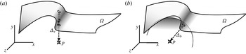
. A sketch is given in figure 9(a), emphasising that even if the line used to measure distance crosses the interface multiple times, only the highest intersection is used. It should be noted that discarding the lower intersections hides part of the complexity of the interface, and that most handles and pockets are not captured. This criterion has been used to study the T/NT interface in boundary layers by Chauhan et al. (Reference Chauhan, Philip, de Silva, Hutchins and Marusic2014) using normals to the wall, and in jets by Westerweel et al. (Reference Westerweel, Fukushima, Pedersen and Hunt2009) and da Silva & Taveira (Reference da Silva and Taveira2010) using normals to the symmetry plane.
Sketch of (a) the vertical distance
 ${\it\Delta}_{v}$
and (b) the ball distance
 ${\it\Delta}_{b}$
between a point
 $p$
and a surface
 ${\it\Omega}$
. In the case of
 ${\it\Delta}_{v}$
, the wall-normal line may intersect
 ${\it\Omega}$
multiple times, but only the top intersection is kept. Here, the surface has a pocket and the line crosses it three times. In the case of the ball distance, there is usually only one point where the sphere centred at
 $p$
with radius
 ${\it\Delta}_{b}$
is tangent to
 ${\it\Omega}$
, marked here with a small circle.

Our second definition of distance is the separation between the point
 $p$
and its closest point in
 ${\it\Omega}$
. We will call it the ball (or minimum) distance
 ${\it\Delta}_{b}$
, and it has a simple geometrical interpretation as the radius of the sphere tangent to the interface and centred at
 $p$
. It is sketched in figure 9(b). Some properties of this distance are particularly convenient for a conditional analysis. Regardless of the complexity of the surface, there is always a closest surface point to any point in space, and the ball distance is always uniquely defined. If the point
 $p$
is infinitesimally close to the interface,
 ${\it\Delta}_{b}$
is equivalent to the distance measured along the local normal. It also has a relatively simple mathematical formulation, since it satisfies the Eikonal equation
 $|\boldsymbol{{\rm\nabla}}({\it\Delta}_{b})|=1$
with
 ${\it\Delta}_{b}=0$
at the interface. This equation has a solution regardless of the complexity of the boundary condition, and can be integrated by several fast methods (Jones, Baerentzen & Sramek Reference Jones, Baerentzen and Sramek2006).
The relation between the two distance definitions depends on the local orientation and complexity of the surface. Referring to figure 10(a), when the T/NT interface is mostly horizontal, simple and smooth, the two definitions produce similar results. When the interface is more complex or is not parallel to the wall, as in figure 10(b), the two results are different. For example, point
 $p$
in figure 10(b) is very close to the interface in terms of
 ${\it\Delta}_{b}$
, but relatively deep into the turbulent side in terms of
 ${\it\Delta}_{v}$
.
Other authors have introduced alternative definitions of conditional distance. da Silva & Pereira (Reference da Silva and Pereira2008) and Watanabe et al. (Reference Watanabe, Sakai, Nagata, Ito and Hayase2015) use the local normal to the interface, obtained in two and three dimensions respectively. This is similar to the ball distance close to
 ${\it\Delta}=0$
, particularly in the three-dimensional case, but farther away normals may intersect each other, and the two definitions are not comparable. There have been efforts to study the conditional properties of the interface using Lagrangian trackers in jets (Holzner et al.
Reference Holzner, Liberzon, Nikitin, Lüthi, Kinzelbach and Tsinober2008; Taveira et al.
Reference Taveira, Diogo, Lopes and da Silva2013), but the trajectories soon get complicated away from the interface, and Atkinson et al. (Reference Atkinson, Hackl, Stegeman, Borrell and Soria2014) showed that tracking them close to the edge of the boundary layer is significantly more difficult than in jets, where the free-stream velocity is very low.
(a) Sketch of a simple almost horizontal surface for which
 ${\it\Delta}_{v}\simeq {\it\Delta}_{b}$
. (b) Example of a case in which the two distances are very different. Here, point
 $p$
is very close to the interface and
 ${\it\Delta}_{b}\simeq 0$
, but lies underneath a pocket and a handle, and
 ${\it\Delta}_{v}\gg {\it\Delta}_{b}$
.

Our algorithm to obtain the ball distance starts from the set
 ${\it\Omega}_{i}$
of interface voxels defined in (4.1). The vorticity within each voxel is approximated by a trilinear interpolation of the values at the vertices, so that the T/NT interface is approximated by a polyhedron of which each interface voxel contains a planar face. The interface is approximated by the set
 ${\it\Omega}_{p}$
of the points that are closest to the centre of the voxel in each of those faces. The sets
 ${\it\Omega}_{i}$
and
 ${\it\Omega}_{p}$
are illustrated in figure 11.
(a) The set
 ${\it\Omega}_{i}$
of voxels that contain the interface. (b) The set
 ${\it\Omega}_{p}$
of points used to approximate the T/NT interface.

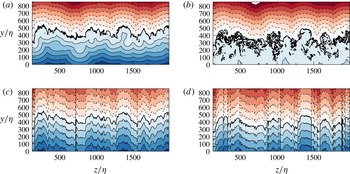
Cross-stream sections of the signed distance fields for the lowest and highest available thresholds, and for the two definitions of distance: (a)
 ${\it\Delta}_{b}$
and
 ${\it\omega}_{0}^{\ast }=0.01$
, (b)
 ${\it\Delta}_{b}$
and
 ${\it\omega}_{0}^{\ast }=0.5$
, (c)
 ${\it\Delta}_{v}$
and
 ${\it\omega}_{0}^{\ast }=0.01$
, (d)
 ${\it\Delta}_{v}$
and
 ${\it\omega}_{0}^{\ast }=0.5$
. All sections correspond to the same flow field at
 ${\it\delta}_{99}^{+}=1500$
. The thicker solid line represents the T/NT interface for each distance definition, and always corresponds to a single connected surface. The isolated spots are due to three-dimensional contortions. Other contour levels are separated by
 $50{\it\eta}$
for
 ${\it\Delta}_{b}$
and by
 $100{\it\eta}$
for
 ${\it\Delta}_{v}$
. Negative contours are dashed.

The ball distance between
 $p$
and
 ${\it\Omega}$
is approximated by the distance between
 $p$
and its nearest neighbour in
 ${\it\Omega}_{p}$
. The nearest-neighbour search (NNS) is a common problem in optimisation. If
 $N_{p}$
is the number of elements in the set
 ${\it\Omega}_{p}$
, a fast solution requiring
 $O(\log N_{p})$
computations was found by Arya et al. (Reference Arya, Mount, Netanyahu, Silverman and Wu1998). Most data analysis packages and toolkits provide implementations of some variant of NNS, and free libraries are available (Muja & Lowe Reference Muja and Lowe2014). By convention, the distance to the interface is defined as positive or negative depending on whether the point
 $p$
has been classified as being in the turbulent or the non-turbulent region. It should be noted that, because the distance is computed with respect to the cleaned interface defined in § 4.1, turbulent and non-turbulent points refer to the smoothed flow regions. Bubbles are counted as turbulent and drops as non-turbulent.
In our analysis, the ball distance is treated as a field and is computed for all the collocation points in the computational grid. Assuming a total number
 $N$
of grid points, obtaining the field of ball distances requires
 $O(N\log N_{p})$
operations. For our data,
 $N_{p}$
is of the order of
 $10^{8}$
, and
 $N$
is of the order of
 $10^{9}$
for each snapshot. The same procedure is followed for the vertical distance
 ${\it\Delta}_{v}$
, with a computational cost of
 $O(N)$
.
5.1 The signed distance field
The discrete fields obtained with the minimum and vertical distances are called the ball-distance field
 ${\it\Delta}_{b}(x,y,z)$
and the vertical-distance field
 ${\it\Delta}_{v}(x,y,z)$
respectively. The symbol
 ${\it\Delta}$
denotes distance regardless of the particular definition.
The concept of a distance field is also found in Mellado, Wang & Peters (Reference Mellado, Wang and Peters2009), who use the length of the trajectories along lines of maximum gradient of an advected scalar to measure the distance with respect to the interface. While their definition can also be used regardless of the complexity of the surface, the gradient lines of the vorticity magnitude become very contorted away from the interface on the turbulent side, and less suitable for conditional analysis than either of the two definitions mentioned above.
Sections of the two distance fields of the same snapshot of the flow are shown in figure 12, each computed for two different thresholds. The isosurface
 ${\it\Delta}=0$
is our effective definition of the interface, but note that the two distance definitions generate different surfaces. The first observation is that the two distances give fairly different results on the turbulent side, particularly for the higher vorticity thresholds. On the non-turbulent side, where the interface is more convex, the differences are not as important. When the threshold is within the topological transition, such as
 ${\it\omega}_{0}^{\ast }=0.5$
in figure 12(b,d), the contortions of the ‘ball’ interface are so intense that there are very few points on the turbulent side for which
 ${\it\Delta}_{b}>100{\it\eta}$
. We emphasise that
 ${\it\Delta}_{b}=0$
in figure 12(b) corresponds to a single connected surface from which bubbles have been removed, and that the apparently isolated contours within the turbulent side are artefacts of the two-dimensional section. Comparison of the results of the two thresholds for each distance definition shows that the vertical-distance field in figure 12(c,d) is less sensitive to the contortions than the ball distance in figure 12(a,b), and also less sensitive to the choice of the threshold. Because of this, it misses most of the interface complexity and the existence of the topological transition.
Away from the wall, the two distance definitions also behave differently. Because of its connection with the Eikonal, the ball distance can be visualised as a wavefront moving away from the interface at a uniform velocity. As is does, the interface irregularities are eliminated by successive mergings of caustics, and the
 ${\it\Delta}_{b}$
isosurface becomes smoother. Roughly speaking, a
 ${\it\Delta}_{b}$
isosurface only retains wavelengths larger than
 $O(|{\it\Delta}_{b}|)$
. The vertical distance does not share this smoothing property. Because the
 ${\it\Delta}_{v}$
isosurfaces are vertical translations of the interface, they retain its irregularities at all distances. It should be noted also that neither distance is additive. Because a
 ${\it\Delta}\neq 0$
isosurface is not an iso-vorticity surface, even if the
 ${\it\Delta}=0$
surface is defined as one, it is impossible to define a distance between interfaces with different thresholds such that
 ${\it\Delta}(p\rightarrow {\it\omega}_{0})={\it\Delta}(p\rightarrow {\it\omega}_{1})+{\it\Delta}({\it\omega}_{1}\rightarrow {\it\omega}_{0})$
. This will later lead to ambiguities in the definition of the thickness of the T/NT interface layer.
The angle
 ${\it\theta}$
between the normal to the
 ${\it\Delta}_{b}$
interface and the vertical can be estimated by
 $\text{d}{\it\Delta}_{v}/\text{d}{\it\Delta}_{b}|_{{\it\Delta}_{b}=0}=1/\cos {\it\theta}$
, but there is no simple way to evaluate the orientation of the
 ${\it\Delta}_{v}$
interface in this manner.
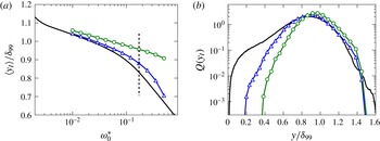
(a) Mean position of the T/NT interface as a function of the vorticity threshold. No symbols, vorticity isosurface as in figure 4; ▵, interface defined as
 ${\it\Delta}_{b}=0$
; ○,
 ${\it\Delta}_{v}=0$
. The threshold in (b) is the vertical dashed line. (b) The PDFs of the vertical positions of the three isosurfaces for
 ${\it\omega}_{0}^{\ast }=0.19$
. The lines are as in (a);
 ${\it\delta}^{+}=1500$
.

None of the interfaces defined by the above distance criteria exactly coincide with a vorticity isosurface. In the case of
 ${\it\Delta}_{b}$
the only difference is the absence of the bubbles and drops discarded in the smoothing step, and the deviations are relatively minor. The vertical distance misses substantial parts of the isosurface, and may deviate significantly from it. Figure 13(a) shows the mean positions of the two interfaces as a function of
 ${\it\omega}_{0}^{\ast }$
, compared with the mean position of the vorticity isosurface. The mean
 $\langle y_{I}({\it\Delta}_{b})\rangle$
deviates little from the position
 $\langle y_{I}\rangle$
of the vorticity isosurface (figure 4), but
 $\langle y_{I}({\it\Delta}_{v})\rangle$
remains close to the edge of the boundary layer even when the vorticity isosurface moves closer to the wall. This is confirmed by the PDFs of the heights of the three isosurfaces, given in figure 13(b). For low thresholds (not shown), the PDFs of the two interfaces and of the vorticity isosurface roughly coincide, and are approximately Gaussian (Corrsin & Kistler Reference Corrsin and Kistler1955). However, for the higher threshold in figure 13(b),
 $y_{I}({\it\Delta}_{b})$
follows the isosurface into the turbulent core of the boundary layer substantially better than
 $y_{I}({\it\Delta}_{v})$
. As a consequence,
 $y_{I}({\it\Delta}_{b})$
results in a much better representation of the intermittency parameters of the boundary layer, such as
 ${\it\gamma}$
. It should be noted that the vorticity threshold used in figure 13(b),
 ${\it\omega}_{0}^{\ast }=0.19$
, although relatively high, is below the topological transition, and in the range of most of the studies collected in table 2.
5.2 Conditional analysis of distance and vorticity
The properties of the vorticity conditioned to its position with respect to the interface can be analysed using the joint PDF of the vorticity magnitude and the distance,
 $F_{{\it\omega},{\it\Delta}}$
. Figure 14 shows four examples corresponding to the thresholds and distance definitions in figure 12. Similar PDFs were obtained by Taveira & da Silva (Reference Taveira and da Silva2014) using
 ${\it\Delta}_{v}$
in a planar jet, and by da Silva et al. (Reference da Silva, Taveira and Borrell2014b
) for jets, a shearless interface and a subset of the present boundary layer. The analysis in the present paper has been carried out for five Reynolds numbers in the range
 ${\it\delta}_{99}^{+}\in (1100{-}1900)$
, and 10 thresholds in
 ${\it\omega}_{0}^{\ast }\in (0.01{-}0.5)$
, each of them computed for the two distance definitions described above.
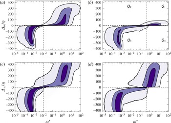
Premultiplied joint PDF of vorticity and distance,
 ${\it\omega}F_{{\it\omega},{\it\Delta}}$
. Each panel corresponds to the thresholds, Reynolds number and distance definitions in figure 12 ((a,b)
 ${\it\Delta}_{b}$
, (c,d)
 ${\it\Delta}_{v}$
, (a,c)
 ${\it\omega}_{0}^{\ast }=0.01$
, (b,d)
 ${\it\omega}_{0}^{\ast }=0.5$
). The contours contain 50 %, 90 % and 99 % of points.

The joint PDF can be divided into four quadrants (figure 14
b), separated by the axes
 ${\it\Delta}=0$
and
 ${\it\omega}={\it\omega}_{0}$
, marked with dashed lines in figure 14. Given that the flow field is the same in the four figures, the differences in the joint PDF are due to the different distance definitions and thresholds.
The first quadrant, which contains points classified as turbulent and with a relatively high vorticity, represents the core turbulent flow. As already seen in figure 12, the minimum and vertical distances behave similarly for low thresholds (figure 14
a,c), but very differently for thresholds within the topological transition. The field of vertical distances depends only slightly on the threshold (figure 14
c,d), but there are few points at distances beyond
 ${\it\Delta}_{b}=100{\it\eta}$
for the higher threshold in figure 14(b).
The second quadrant contains different geometrical objects depending on the distance definition. It contains bubbles for
 ${\it\Delta}_{b}$
, and bubbles, handles and pockets for
 ${\it\Delta}_{v}$
. For the ball distance, the weight of the second quadrant is always small compared with the first one, and contributes little to the averaged vorticity on the free-stream side of the interface (figure 14
a,b). This is not the case for the vertical distance, and it is clear from figure 14(c,d) that the weight of this quadrant increases as the interface becomes more complex at high thresholds. This quadrant, with special reference to the properties of the pockets, will be studied in more detail in § 5.4.
The third quadrant contains points of low vorticity classified as non-turbulent. It represents the bulk of the free stream which, in the case of
 ${\it\Delta}_{b}$
, also includes the irrotational pockets. It depends only weakly on the threshold and on the distance definition, except for
 ${\it\omega}\approx {\it\omega}_{0}$
.
The fourth quadrant, with
 ${\it\omega}>{\it\omega}_{0}$
and negative distances, corresponds to the objects defined in § 4.1 as drops. It is almost empty for all of the cases considered in this study, confirming that the smoothing of the free stream described in § 4.1 does not affect the results of the conditional analysis.
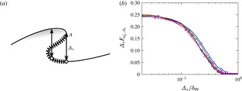
(a) Sketch of the discontinuity of the vertical distance at the edge of a pocket. The hatched line marks points where
 ${\it\omega}={\it\omega}_{0}$
and
 ${\it\Delta}_{b}=0$
, but
 ${\it\Delta}_{v}>0$
. The non-turbulent region just outside
 $A$
has
 ${\it\Delta}_{b}\simeq 0$
but
 ${\it\Delta}_{v}<0$
. (b) Premultiplied PDF,
 ${\it\Delta}_{v}F_{{\it\omega}_{0}^{-},{\it\Delta}_{v}}$
, of the vertical distance of the non-turbulent points with
 ${\it\omega}^{\ast }=0.25{-}0.5$
, whose vorticity is close to the threshold
 ${\it\omega}_{0}^{\ast }=0.5$
: ○ (blue),
 ${\it\delta}_{99}^{+}=1100$
;
 $\times$
(green), 1300; ▵ (red), 1500; ▿ (black), 1700;
 $\star$
(magenta), 1900.

The influence of the distance definition on the joint PDF is most visible far from the horizontal axis in the neighbourhood of
 ${\it\omega}={\it\omega}_{0}$
. These are points in which the vorticity is close to the identification isosurface, but which are incorrectly identified as being far from the interface. The range of possible ball distances for
 ${\it\omega}\simeq {\it\omega}_{0}$
(figure 14
a,b) is very narrow,
 $|{\it\Delta}_{b}|<100{\it\eta}$
, especially in the second quadrant, and can be interpreted as a typical distance to the interface of the irrotational bubbles that have been labelled as turbulent by the smoothing process. On the other hand, the vertical distances in the same region can be as large as
 $250{\it\eta}$
on both sides of the interface (figure 14
c,d). We denote by
 ${\it\omega}_{0}^{-}$
the vorticities just below the threshold. The wide
 ${\it\Delta}_{v}$
tails of
 $F_{{\it\omega}_{0}^{-},{\it\Delta}_{v}}$
have several causes, sketched in figure 15(a). On the positive side,
 ${\it\Delta}_{v}>0$
in
 $Q_{2}$
, all of the points represented with a hatched line in that figure are on the
 ${\it\omega}={\it\omega}_{0}$
and
 ${\it\Delta}_{b}=0$
isosurfaces, but not on the
 ${\it\Delta}_{v}$
interface, which is only the top of the overhang. Points near the hatched line have vorticities close to
 ${\it\omega}_{0}$
, but are counted as being deep within the turbulent region by
 ${\it\Delta}_{v}$
. The
 ${\it\Delta}_{v}<0$
tail of
 $F_{{\it\omega}_{0}^{-},{\it\Delta}_{v}}$
in
 $Q_{3}$
contains points whose vorticity is slightly below that of the threshold, but which are classified by
 ${\it\Delta}_{v}$
as being far within the irrotational region. They correspond to points such as
 $A$
in figure 15(a), where the orientation of the interface is vertical and induces a discontinuity in the height of the
 ${\it\Delta}_{v}$
interface. Such discontinuities are clearly visible in figure 12(c,d). These tangencies are less common than the overhung surfaces, and the mass in the negative tail of
 $F_{{\it\omega}_{0}^{-},{\it\Delta}_{v}}$
is typically smaller than in the positive one, especially in the convoluted interfaces at the higher thresholds (only 15 % as many in figure 12
d).
It is clear from figure 15(a) that the negative tail of
 $F_{{\it\omega}_{0}^{-},{\it\Delta}_{v}}$
contains information about the ‘depth’ of the pockets, rather than about the thickness of the interface. The premultiplied probability distribution
 ${\it\Delta}_{v}F_{{\it\omega}_{0}^{-},{\it\Delta}_{v}}$
, integrated over the band
 ${\it\omega}\in ({\it\omega}_{0}/2,{\it\omega}_{0})$
, is presented in figure 15(b) for a relatively high threshold. It is well approximated by a power law
 $F_{{\it\omega}_{0}^{-},{\it\Delta}_{v}}\propto {\it\Delta}_{v}^{-1}$
for
 ${\it\Delta}_{v}\lesssim 0.2{\it\delta}_{99}$
. Although the reason for this particular power is not completely clear, it suggests a regular structure for the
 ${\it\Delta}_{v}$
interface. That interface has no overhangs, and renders pockets as holes with steep sides. If we assume that the interface is covered with pockets of size
 ${\it\Delta}$
, the contribution of each hole to the PDF in figure 15(b) would be proportional to the
 $O({\it\Delta})$
length of its lip. Their number would be proportional to
 ${\it\Delta}^{-2}$
and the total lip length would be proportional to
 ${\it\Delta}^{-1}$
, as in the figure.
Even if this explanation turns out to be oversimplified, the fact that the distribution of pocket heights satisfies a power law is consistent with a fractal interface, and suggests that the discontinuities represent a self-similar hierarchy of overhangs. For the threshold in figure 15(b), the self-similar range ends around
 ${\it\Delta}_{v}\approx 0.2{\it\delta}_{99}$
, and the probability of finding pockets deeper than that limit is very low. This is approximately three times the standard deviation of the position of the vorticity isosurface for this threshold (figure 4). At lower thresholds such as those in figure 14(a,c), the self-similar range disappears, and the ‘pocket’ distribution is concentrated around
 ${\it\Delta}_{v}=10{\it\eta}$
.
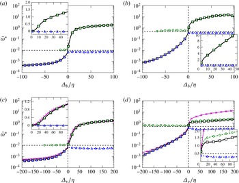
Conditional profiles: – –▫– –,
 $\overline{{\it\omega}}$
; – –○– –,
 $\overline{{\it\omega}_{1}}$
; – –▵– –,
 $\overline{{\it\omega}_{2}}$
. The figures follow the same arrangement as in figure 12 ((a,b)
 ${\it\Delta}_{b}$
, (c,d)
 ${\it\Delta}_{v}$
, (a,c)
 ${\it\omega}_{0}^{\ast }=0.01$
, (b,d)
 ${\it\omega}_{0}^{\ast }=0.5$
). The black dashed lines correspond to the values of the threshold (vertical) and zero distance (horizontal). The inset in each figure corresponds to the same plot, using linear coordinates for the vorticity magnitude. The two solid lines with crosses in (c) and (d) correspond to
 $\overline{{\it\omega}}(3.1{\it\Delta}_{b})$
(see § 5.3.1).

5.3 Conditional averages
The averaged vorticity conditioned to the distance to the interface can be computed from
 $F_{{\it\omega},{\it\Delta}}$
as
 $$\begin{eqnarray}\overline{{\it\omega}}({\it\Delta})=\frac{\displaystyle \int _{0}^{\infty }{\it\omega}F_{{\it\omega},{\it\Delta}}\,\text{d}{\it\omega}}{\displaystyle \int _{0}^{\infty }F_{{\it\omega},{\it\Delta}}\,\text{d}{\it\omega}}.\end{eqnarray}$$
It is given by the solid lines with squares in figure 16(a–d), and is equivalent to the conditional vorticity profiles in Westerweel et al. (Reference Westerweel, Hofmann, Fukushima and Hunt2002). One should note the use of the bar over the symbol to distinguish (5.1) from the more usual mean profile
 $\langle {\it\omega}\rangle$
at a given distance from the wall, defined as
 $$\begin{eqnarray}\langle {\it\omega}\rangle (y)=\frac{\displaystyle \int _{0}^{\infty }{\it\omega}{\it\Gamma}_{{\it\omega},y}\,\text{d}{\it\omega}}{\displaystyle \int _{0}^{\infty }{\it\Gamma}_{{\it\omega},y}\,\text{d}{\it\omega}}.\end{eqnarray}$$
We will use the notation
 $\overline{{\it\omega}}({\it\Delta}_{b})$
and
 $\overline{{\it\omega}}({\it\Delta}_{v})$
to distinguish between conditional profiles obtained with each definition of distance.
The conditional vorticity in all of the panels of figure 16 increases monotonically to its expected fully turbulent level,
 ${\it\omega}^{\ast }=O(1)$
, within a few Kolmogorov lengths from the interface, except for the plateau at
 ${\it\Delta}_{v}/{\it\eta}=15{-}40$
in figure 16(d).
The existence of a plateau or of a maximum in the conditional vorticity profile near the T/NT interface has been mentioned in wakes (Townsend Reference Townsend1976; Bisset et al.
Reference Bisset, Hunt and Rogers2002) and reported in jets (Westerweel et al.
Reference Westerweel, Fukushima, Pedersen and Hunt2009; da Silva et al.
Reference da Silva, dos Reis and Pereira2011). Its presence has sometimes been used to define the thickness of the interface layer (da Silva & Taveira Reference da Silva and Taveira2010), and taken as the basis for theoretical models in which the interface is maintained by the presence of a strong localised shear (Hunt & Durbin Reference Hunt and Durbin1999). Similar models have been used to suggest similarities between the T/NT interface in jets (Westerweel et al.
Reference Westerweel, Fukushima, Pedersen and Hunt2009) and strong internal vortex layers in homogeneous turbulence (Ishihara, Kaneda & Hunt Reference Ishihara, Kaneda and Hunt2013). Chauhan et al. (Reference Chauhan, Philip, de Silva, Hutchins and Marusic2014) report a strong conditional vorticity peak in boundary layers, but their interface is defined in terms of the velocity fluctuations, and we will argue below that it is probably different from the one discussed here. Moreover, not all of these papers use the same definition of the interface or even the same thresholded scalar. In fact, when da Silva et al. (Reference da Silva, Hunt, Eames and Westerweel2014a
) compiled conditional vorticity statistics for a variety of flows, the only obvious peak was found in the early stages of the evolution of a shearless mixing layer (da Silva & Taveira Reference da Silva and Taveira2010). Bisset et al. (Reference Bisset, Hunt and Rogers2002) also find strong-vorticity peaks for some high-vorticity thresholds in their wake, but attribute them to the presence of isolated vorticity patches, and discard them in favour of a lower threshold
 $({\it\omega}^{\ast }\approx 0.1)$
for which the maximum is barely noticeable. Although we will find and discuss below comparable peaks in other variables, we note at this stage that, if the vorticity magnitude were particularly intense close to the interface, a plateau analogous to the one in figure 16(d) should also appear in the
 $\overline{{\it\omega}}({\it\Delta}_{b})$
profile in figure 16(b), but this is not the case. An alternative explanation is that the vorticity close to the interface is not particularly intense, but that, when the conditional profiles are obtained as a function of
 ${\it\Delta}_{v}$
at a sufficiently high threshold, some non-turbulent flow is counted as being turbulent within the inner part of the interface, lowering the local average vorticity (Bisset et al.
Reference Bisset, Hunt and Rogers2002).
To differentiate between the two hypotheses we split the conditional profile
 $\overline{{\it\omega}}({\it\Delta}_{v})$
into contributions from the high-vorticity first quadrant,
 $Q_{1}$
, and the mislabelled non-turbulent points in
 $Q_{2}$
. Equation (5.1) is split into
 $$\begin{eqnarray}\overline{{\it\omega}}=W_{1}\overline{{\it\omega}}_{1}+W_{2}\overline{{\it\omega}}_{2},\end{eqnarray}$$
where
 $$\begin{eqnarray}\overline{{\it\omega}}_{1}=\frac{\displaystyle \int _{{\it\omega}_{0}}^{\infty }{\it\omega}F_{{\it\omega},{\it\Delta}}\,\text{d}{\it\omega}}{\displaystyle \int _{{\it\omega}_{0}}^{\infty }F_{{\it\omega},{\it\Delta}}\,\text{d}{\it\omega}},\quad \overline{{\it\omega}}_{2}=\frac{\displaystyle \int _{0}^{{\it\omega}_{0}}{\it\omega}F_{{\it\omega},{\it\Delta}}\,\text{d}{\it\omega}}{\displaystyle \int _{0}^{{\it\omega}_{0}}F_{{\it\omega},{\it\Delta}}\,\text{d}{\it\omega}}\end{eqnarray}$$
are the conditional averages for
 $Q_{1}$
and
 $Q_{2}$
, and
 $$\begin{eqnarray}W_{1}=\frac{\displaystyle \int _{{\it\omega}_{0}}^{\infty }F_{{\it\omega},{\it\Delta}}\,\text{d}{\it\omega}}{\displaystyle \int _{0}^{\infty }F_{{\it\omega},{\it\Delta}}\,\text{d}{\it\omega}},\quad W_{2}=\frac{\displaystyle \int _{0}^{{\it\omega}_{0}}F_{{\it\omega},{\it\Delta}}\,\text{d}{\it\omega}}{\displaystyle \int _{0}^{\infty }F_{{\it\omega},{\it\Delta}}\,\text{d}{\it\omega}}\end{eqnarray}$$
are the corresponding weights. The profiles of
 $\overline{{\it\omega}}$
,
 $\overline{{\it\omega}}_{1}$
and
 $\overline{{\it\omega}}_{2}$
are given in figure 16. In the case of low thresholds (a,c),
 $\overline{{\it\omega}}_{1}\simeq \overline{{\it\omega}}$
, and the contribution of the second quadrant is small, regardless of the distance definition.
The only case in which
 $\overline{{\it\omega}}_{1}$
is clearly different from the overall average is figure 16(d), in which the contribution of the handles and pockets is significant. In this figure, the maximum relative weight of
 $Q_{2}$
is
 $W_{2}\simeq W_{1}/4$
at
 ${\it\Delta}_{v}=20{\it\eta}$
. At the even higher thresholds at which the interface reaches its maximum geometrical complexity near the end of the topological transition, the weights of the two quadrants are comparable. This has a noticeable effect on the conditional profiles, and it is clear from figure 16(d) that the plateau is a consequence of the negative contribution from
 $\overline{{\it\omega}}_{2}$
. If we consider this contribution as a spurious effect of
 ${\it\Delta}_{v}$
, the ‘true’ conditional vorticity
 $\overline{{\it\omega}}_{1}$
in figure 16(d) increases monotonically near the interface. In essence, the conditional vorticity remains constant or decreases away from the interface because
 ${\it\Delta}_{v}$
misclassifies some weakly vortical pockets as part of the turbulent flow.
Conditional vorticity profiles for
 ${\it\delta}_{99}^{+}=1900$
, computed as in figure 16, as functions of the threshold: ○,
 ${\it\omega}_{0}^{\ast }=0.17$
; ▫, 0.29; ▵, 0.52; ▿, 0.88; (a)
 ${\it\Delta}_{v}$
, (b)
 ${\it\Delta}_{b}$
.

This effect is clearer in figure 17, which presents conditional vorticities for several interface thresholds. Figure 17(a) is computed with
 ${\it\Delta}_{v}$
, and develops a plateau and eventually a peak as the threshold increases. As in figure 16(d), it can be shown that this is a due to the increasingly negative contribution from the pockets as the complexity of the interface increases. Figure 17(b) presents the same cases computed for
 ${\it\Delta}_{b}$
, and shows no trace of an interface peak.
It should be noted that the distances in figure 17(b) are much lower than in figure 17(a), while the conditional vorticities are higher. In fact, similar conditional vorticities are found when the horizontal axis of figure 17(a) is extended to
 ${\it\Delta}_{v}\simeq 400$
, carrying the plot to the neighbourhood of the wall. The plot of
 $\overline{{\it\omega}}({\it\Delta}_{v})$
for these large distances is very similar to a shifted version of
 ${\it\omega}^{\prime }(y)$
(figure 3
a). The vorticity isosurface at these high thresholds permeates the whole boundary layer, and occasionally comes very close to the wall. The ball distance recognises this fact and brings the strong near-wall vorticity closer to the interface, while the vertical distance misses that complexity.
This discussion suggests that the apparent strongly vortical interface layer observed in some of the studies mentioned above either is an artefact of how a one-dimensional definition of distance interacts with a fully three-dimensional geometry or is only manifested in variables different from the vorticity magnitude. In the present case, the above arguments show that the interface peak is due to the neglect of the effect of irrotational pockets on the conditional quantities. We next discuss the relevance of these pockets in the entrainment process.
5.3.1 An approximate relation between
 ${\it\Delta}_{v}$
and
${\it\Delta}_{b}$


A property of the ball distance that can be used to approximately relate it to the more common vertical definition
 ${\it\Delta}_{v}$
is that, sufficiently close to the interface, it corresponds to the distance along the local normal. In consequence, both definitions are related by
 $$\begin{eqnarray}\lim _{{\it\Delta}_{b}\rightarrow 0}{\it\Delta}_{b}/{\it\Delta}_{v}=\cos {\it\theta},\end{eqnarray}$$
where
 ${\it\theta}$
is the angle between the local normal and the vertical direction. Equation (5.6) can be averaged, giving a quantitative relationship between the conditional profiles,
 $$\begin{eqnarray}\overline{\frac{{\it\Delta}_{b}}{{\it\Delta}_{v}}}\sim \overline{\cos {\it\theta}},\end{eqnarray}$$
showing that conditional profiles obtained in terms of the ball distance are
 $\overline{\cos {\it\theta}}$
narrower than those expressed in terms of the vertical distance. The profile
 $\overline{{\it\omega}}({\it\Delta}_{b}/\overline{\cos {\it\theta}})$
is represented in figure 16(c,d) as a magenta line with crosses. Whenever
 $\overline{{\it\omega}}({\it\Delta}_{b}/\overline{\cos {\it\theta}})\simeq \overline{{\it\omega}}({\it\Delta}_{v})$
, the projection of one distance onto the other is quantitatively valid. The results suggest that the two measures are comparable if the geometry of the interface is only moderately complex. For example, figure 16(c) shows that the range of validity of (5.6) for low vorticity thresholds extends to a substantial portion of the boundary-layer thickness, using
 $\overline{\cos {\it\theta}}=0.32$
. On the other hand, when the threshold approaches the topological transition, the two measurements are only comparable within a region very close to the interface (figure 16
d).
Although this relationship between
 ${\it\Delta}_{b}$
and
 ${\it\Delta}_{v}$
is only a gross approximation, it contains information about the shape of the interface. Lower values of
 $\overline{\cos {\it\theta}}$
imply that the interface is steeper on average, so that the local normal is less likely to be aligned with the vertical axis. To give some perspective on the empirical 0.32 factor mentioned above, the same result for a hemisphere yields
 $\overline{\cos {\it\theta}}=0.5$
.
5.4 The relevance of pockets
We saw in figure 15 that pockets form a self-similar hierarchy of many different sizes, and it has been conjectured that their formation signals the large-scale engulfment of irrotational fluid before it is finally entrained by small-scale ‘nibbling’. Their abundance has been used to quantify the relative importance of the two processes (Sandham et al. Reference Sandham, Mungal, Broadwell and Reynolds1988; Mathew & Basu Reference Mathew and Basu2002).
Flow within pockets of the interface at
 ${\it\omega}_{0}^{\ast }=0.5$
: – – –,
 ${\it\delta}_{99}^{+}=1100$
; ——,
 ${\it\delta}_{99}^{+}=1900$
. (a) Joint PDF of
 ${\it\Delta}_{v}$
and
 ${\it\Delta}_{b}$
within the region. The two contours for each Reynolds number contain 60 % and 98 % of the points. (b) Average vorticity within the pockets as a function
 ${\it\Delta}_{v}$
and
 ${\it\Delta}_{b}$
within the region that contains 98 % of the points. The contours are
 ${\it\omega}^{\ast }=0.15$
, 0.25, 0.35. The two red diagonals are
 ${\it\Delta}_{v}={\it\Delta}_{b}$
.

We can define pockets as regions identified by the ball distance as part of the free stream,
 ${\it\Delta}_{b}<0$
, and by the vertical distance as turbulent,
 ${\it\Delta}_{v}>0$
. For the purpose of this section, they include the undersides of handles as well as simple folds of the interface. Figure 18(a) shows the joint PDF of the two distances in the range corresponding to pockets. The figure is drawn for the relatively high vorticity threshold of figure 12(b,d), guaranteeing both the presence of abundant pockets and the possibility of observing how the vorticity diffuses into the irrotational flow. It includes the two extreme Reynolds numbers in our simulation, allowing some scaling comparisons. For instance, the agreement between the two profiles of
 $\langle y_{I}\rangle$
suggests that the thickness of the intermittent region is not expected to change substantially with higher Reynolds numbers. It turns out that the size of the pockets, as measured by the maximum
 ${\it\Delta}_{b}$
, scales best in terms of the Taylor microscale, while their depth within the layer, as measured by
 ${\it\Delta}_{v}$
, scales better with the boundary-layer thickness. The joint PDF is roughly triangular. It is bounded on the left by the trivial limit
 ${\it\Delta}_{b}\leqslant {\it\Delta}_{v}$
, plotted for each Reynolds number as a thick inclined straight line, and on the right by a roughly hyperbolic curve which can be interpreted to mean that deeper pockets (large
 ${\it\Delta}_{v}$
) tend to be smaller (small
 ${\it\Delta}_{b}$
), presumably because they have been broken down by the turbulence while being entrained.
The question of whether being entrained into a pocket also promotes the diffusion of vorticity is tested in figure 18(b), which shows the distribution of the conditionally averaged vorticity in the same parameter space as figure 18(a). It should be noted that all of the vorticity levels in this figure are below the interface threshold, so that the band of higher vorticities along the top of figure 18(b) portrays how vorticity diffuses into the irrotational fluid. It should be noticed that the size of the pockets in this figure is normalised with
 ${\it\eta}$
. Comparison with figure 18(a) shows that the difference between scaling it with
 ${\it\eta}$
or
 ${\it\lambda}$
is not great, but the collapse of the vorticity band at the top of figure 18(b) is considerably better with
 ${\it\eta}$
than with
 ${\it\lambda}$
. Its width, approximately
 $5{-}10{\it\eta}$
, strongly suggests a viscous origin (van Reeuwijk & Holzner Reference van Reeuwijk and Holzner2014), and it is clear from the figure that the vorticity is correlated with the ball distance, but not with the vertical position with respect to the interface. The only exceptions are points near the line
 ${\it\Delta}_{v}={\it\Delta}_{b}$
, where the two measures coincide.
The implication is that the fluid within pockets is sensitive to how close it is to the interface, but not to how deep it is within the turbulent layer. If engulfment were an important mechanism to promote the diffusion of vorticity into the irrotational fluid, for example by preferentially straining it, one would expect some correlation between
 ${\it\Delta}_{v}$
and the width of the diffusion band at the top of figure 18(b), but there is little evidence for that. Apparently, whether the fluid is within a pocket or not is immaterial to its behaviour, although the breakup of the deeper pockets into smaller sizes should enhance the overall effect of viscous diffusion. We will only use
 ${\it\Delta}_{b}$
from now on in our analysis.
Premultiplied joint PDF,
 ${\it\omega}F_{{\it\omega},{\it\Delta}_{b}}$
, of the vorticity and ball distance on the turbulent side of the interface for (a) a low threshold,
 ${\it\omega}_{0}^{\ast }=0.01$
, and (b) a moderate one at the beginning of the topological transition,
 ${\it\omega}_{0}^{\ast }=0.09$
. Two Reynolds numbers are presented in each panel,
 ${\it\delta}_{99}^{+}=1100$
(—— black) and
 ${\it\delta}_{99}^{+}=1900$
(– – – blue). The vertical solid line is
 ${\it\omega}_{0}^{\ast }$
. (c,d) Same as (a,b), but with the vorticity in wall units and the distance normalised with the boundary-layer thickness. The horizontal bar is the variation of
 ${\it\omega}^{\ast }/{\it\omega}^{+}$
in our range of
 ${\it\delta}_{99}^{+}$
. The curves with markers correspond to the average vorticity magnitudes for each Reynolds number,
 ${\it\delta}_{99}^{+}=1900$
(green ▵) and
 ${\it\delta}_{99}^{+}=1100$
(magenta ○). The contours contain 50 %, 90 % and 99 % of points.

5.5 The interface layer
While the previous sections deal with the properties of the interface surface, it is also interesting to characterise the properties of the interface layer, understood as the part of the turbulent flow that is directly influenced by its proximity to the free stream. As a first step, figure 19(a,b) reproduces the first and second (turbulent) quadrants of the joint PDFs of the vorticity and distance in figure 14(a,b). The distance axis is now logarithmic, to emphasise the region close to the interface, and each panel includes the two extreme Reynolds numbers in our data set.
Three regions can be distinguished in order of increasing distance from the interface. The first and closest to the interface contains the strongest vorticity gradients. A precise definition of the thickness of this layer will be given in § 5.7, but, if we define the limit of this layer by the intersection of two straight lines tangent to the probability isocontours near and far from the interface, its thickness is of the order of a few Kolmogorov units for the different Reynolds numbers, suggesting a viscous origin. However, this thickness depends on the identification threshold. It is approximately
 $10{\it\eta}$
in figure 19(a)
 $({\it\omega}_{0}^{\ast }=0.01)$
,
 $5{\it\eta}$
in figure 19(b)
 $({\it\omega}_{0}^{\ast }=0.09)$
, and almost vanishes at the beginning of the topological transition,
 ${\it\omega}_{0}^{\ast }=0.2$
(not shown). In the cases in which this region can be identified in the joint PDF, its limit is
 $\overline{{\it\omega}}^{\ast }\approx 1$
, which we have seen above to be the level of fully developed turbulence.
The viscosity-dominated region just outside the interface has been recently studied by van Reeuwijk & Holzner (Reference van Reeuwijk and Holzner2014) and Taveira & da Silva (Reference Taveira and da Silva2014) in temporally evolving turbulence fronts. They identify it with the ‘superlayer’ conjectured by Corrsin & Kistler (Reference Corrsin and Kistler1955), and find that its characteristic thickness is the Kolmogorov microscale computed with the energy dissipation rate of the core flow. The enstrophy level in this viscous layer depends somewhat on the definition, but is typically very low. The viscous region in figure 19 is probably not the superlayer, whose observation requires a higher numerical resolution and a quieter free stream than those in our simulation (van Reeuwijk & Holzner Reference van Reeuwijk and Holzner2014). We will see below that both the rate of strain and the vortex stretching remain high in the viscous layer of figure 19, and that this region is probably best interpreted as part of the ‘buffer layer’ defined by van Reeuwijk & Holzner (Reference van Reeuwijk and Holzner2014) in the range
 ${\it\omega}^{\ast }\in (0.1{-}1)$
. In analogy to the similarly named layer in wall-bounded turbulence, both nonlinear and viscous effects are important in this region. It is interesting that such a hybrid mechanism was proposed by Townsend (Reference Townsend1976), who noted that viscous diffusion of vorticity and its tangential transport should be comparable near the interface. On the assumption of homogeneity, the magnitude of the rate of strain is proportional to the enstrophy, and the predicted result of this mechanism is also a thickness of
 $O({\it\eta})$
.
The region beyond the buffer interface layer is self-similar, in the sense that both the conditionally averaged vorticity and the probability isocontours follow power laws in
 ${\it\Delta}_{b}$
. This implies that there is no intrinsic length or vorticity scale, which is consistent with the intuitive idea of an inertial layer but difficult to interpret dynamically. In the first place, different parts of the PDF scale differently. The strong-vorticity isocontours to the right of figure 19(a) are almost vertical
 $({\it\omega}\propto {\it\Delta}_{b}^{0})$
, but those corresponding to weak vorticity on the left of the figure follow
 ${\it\omega}\propto {\it\Delta}_{b}^{1}$
, and the conditional mean enstrophy approximately satisfies
 ${\it\omega}\propto {\it\Delta}_{b}^{1/2}$
. In the second place, these slopes change with the detection threshold, and it is hard to distinguish any power law in figure 19(b) or at higher thresholds. We mentioned with regard to (3.2)–(3.3) that
 $\langle {\it\omega}\rangle \propto y^{-1/2}$
is a consequence of the local energy equilibrium and the logarithmic profile in the logarithmic layer, but the same argument cannot be used here. The interface is not an impermeable boundary that limits the size of eddies as the wall does, although it could be argued that the size of the eddies defines the position of the interface. The trend in figure 19(a), that larger eddies have more intense vorticity, is contrary to the inertial relation of homogeneous turbulence,
 ${\it\omega}\propto {\it\Delta}^{-2/3}$
(Kolmogorov Reference Kolmogorov1941), and the most plausible explanation is that larger eddies reach closer to the wall and are therefore stronger. The apparent self-similarity in figure 19 may be coincidental.
The width of this intermediate region depends on the identification threshold, but scales with the boundary-layer thickness. It extends to the hockey stick at the top of the PDFs, which contains the points with the highest vorticity and farthest from the interface. This last region is mostly formed by points near the wall. When
 ${\it\omega}$
is scaled in wall units and
 ${\it\Delta}_{b}$
is normalised with the boundary-layer thickness, as in figure 19(c,d), the two Reynolds numbers collapse well for long distances and high vorticities. At the two Reynolds numbers in figure 19,
 ${\it\delta}_{99}/{\it\eta}\approx 250$
and 450.
5.6 Other velocity gradients
In the previous sections, we have discussed the properties of the vorticity field near a vorticity isosurface, and it is perhaps not surprising that they may be special. For example, an interesting question is whether the vorticity within the interface layer has different properties from the core of the turbulent flow, such as perhaps being weaker because it is less strained, but such questions are hard to answer if the interface is defined by the magnitude of the vorticity itself. It is useful for that purpose to determine the conditional properties of other quantities besides the one being thresholded. In this section we study the properties of the strain-rate tensor
 $\unicode[STIX]{x1D64E}$
in the neighbourhood of the vorticity interface, as well as the behaviour of the vorticity in the neighbourhood of an interface defined in terms of the strain. We define
 $S$
as the Euclidean norm of the rate-of-strain tensor,
 $S=\Vert \unicode[STIX]{x1D64E}\Vert$
. In analogy to (3.4), and taking into account that
 $$\begin{eqnarray}\langle {\it\omega}^{2}\rangle =2\langle S^{2}\rangle\end{eqnarray}$$
in homogeneous flows, the star units for
 $S$
are defined as
 $$\begin{eqnarray}S^{\ast }=S\frac{{\it\nu}\sqrt{2{\it\delta}_{99}^{+}}}{u_{{\it\tau}}^{2}}.\end{eqnarray}$$
Equation (5.8) then becomes
 $\langle {\it\omega}^{2}\rangle ^{\ast }=\langle S^{2}\rangle ^{\ast }$
, and suggests that
 ${\it\omega}^{\ast }$
and
 $S^{\ast }$
should be of the same order. The joint PDFs of
 $S$
and
 $y$
, and of
 ${\it\omega}$
and
 $y$
, are presented in figure 20.
Premultiplied joint PDFs: —— (black),
 $S{\it\Gamma}_{y,S}$
; – – – (blue),
 ${\it\omega}{\it\Gamma}_{y,{\it\omega}}$
. The contours contain 50 %, 90 % and 99 % of points. The dashed diagonal is the exponential decay of the Fourier modes of irrotational strain with a wall-parallel wavelength
 $2{\it\delta}_{99}$
.

Both PDFs agree within the turbulent region in the right-lower corner of figure 20, supporting the normalisation (5.9), but the vorticity in the free stream on the left-hand side of the figure is almost two orders of magnitude lower than the rate of strain. This is not unexpected in a nominally irrotational part of the flow but, since (5.8) is a kinematic relation whose only condition is spacial homogeneity, the mismatch between the two magnitudes implies that the strain in the free stream is an inhomogeneous residual effect of the vortical flow within the boundary layer.
Any solenoidal velocity field can be written as
 $$\begin{eqnarray}\boldsymbol{u}=\boldsymbol{{\rm\nabla}}\wedge \boldsymbol{B}+\boldsymbol{{\rm\nabla}}{\it\phi},\end{eqnarray}$$
where the potentials satisfy
 ${\rm\nabla}^{2}{\it\phi}=0$
and
 ${\rm\nabla}^{2}\boldsymbol{B}=-{\bf\omega}$
(Batchelor Reference Batchelor1967). In the irrotational free stream, both potentials satisfy Laplace’s equation and, if they are expanded in terms of wall-parallel Fourier harmonics, decay away from the wall as
 $\exp (-ky)$
, where
 $k^{2}=k_{x}^{2}+k_{z}^{2}$
is the magnitude of the wall-parallel wavevector. All of the velocity components and the rate-of-strain tensor decay exponentially at the same rate, and the slowest decay corresponds to the largest horizontal wavelengths. It is known that this results in an algebraic decay of the velocity fluctuations for
 $y\gg {\it\delta}_{99}$
, because different distances are dominated by different wavenumbers in the long-wavelength end of the spectrum (Phillips Reference Phillips1955; Stewart Reference Stewart1956), but the near field is controlled by the peak of the
 $v$
spectrum in the turbulent region. The thick dashed diagonal in figure 20 is
 $S\propto \exp (-{\rm\pi}y/{\it\delta}_{99})$
, corresponding to the decay of irrotational velocity fluctuations due to structures within the boundary layer whose shortest dimension is
 $O(2{\it\delta}_{99})$
. This is the order of magnitude of the largest structures in boundary layers (Sillero et al.
Reference Sillero, Jiménez and Moser2014).
The vorticity is unrelated to the velocity potentials, and decays much faster than the rate of strain as it enters the free stream. In fact, this was one of the reasons why we originally chose vorticity over other quantities to characterise the T/NT interface.
It should be noted that the vorticity also decays exponentially with
 $y$
in the free stream, although at a much lower absolute level than
 $S$
. This is not a kinematic result, but a consequence of the numerical inflow conditions, which determine the three velocities at the inflow but not their derivatives with respect to
 $x$
. The result is that there is a residual vorticity in the free stream due to terms like
 $\partial _{x}v$
, which inherits the exponential decay of the velocity potentials at the inflow plane.
(a) Fractal dimension and (b) genus of an interface defined by thresholding the norm of the strain-rate tensor: ○,
 ${\it\delta}_{99}^{+}=1100$
;
 $\times$
, 1300; ▿, 1500; ▵, 1700;
 $\star$
, 1900. The horizontal bar is the variation of
 ${\it\omega}^{\ast }/{\it\omega}^{+}$
in our range of
 ${\it\delta}_{99}^{+}$
.

A consequence of the relatively high strain levels in the free stream is that the separation between its characteristic values on the turbulent and non-turbulent sides is not as clear-cut as in the case of the vorticity. Even so, the complexity transition happens at comparable thresholds. The geometrical properties of the strain interface are presented in figure 21. The fractal dimension in figure 21(a) should be compared with figure 7(b) for the vorticity interface. The strain isosurface is smoother, with minimum values close to the non-fractal value,
 $D\approx 2$
. The maximum dimension is also somewhat lower than for the vorticity, in agreement with the observation by Moisy & Jiménez (Reference Moisy and Jiménez2004) that strong dissipation structures are less fractal (plate-like) than those of vorticity (string-like). The evolution of the genus in figure 21(b) is also similar to the case of the vorticity, although the maximum genus and fractal dimension are reached for slightly higher thresholds,
 $S_{0}^{\ast }\approx 2.5$
instead of
 ${\it\omega}_{0}^{\ast }\approx 1.5$
. The topological transition is also narrower for the strain interface, especially for the genus in figure 21(b), which starts to increase at
 $S_{0}^{\ast }\approx 1$
instead of at
 ${\it\omega}_{0}^{\ast }\approx 0.3$
, as it did in figure 8(a). The reason is probably that, while the maximum dimension and genus mark the threshold for which the interface has fully moved into the core turbulent flow, the slower decay of the strain fluctuations with
 $y$
means that low-strain isosurfaces are farther from the wall than for similar enstrophy thresholds, and the corresponding interface becomes regular much faster.
The evolutions of the conditional statistics of the flow across the vorticity and strain isosurfaces are compared in figure 22. The two thresholds chosen are
 $S_{0}^{\ast }=0.1$
and
 ${\it\omega}_{0}^{\ast }=0.01$
, both of which are within the plateau that separates the values of turbulent and non-turbulent flow in their joint PDFs, and well below the beginning of the respective topological transitions. The average height of the resulting interfaces is
 $\langle y_{I}\rangle \approx 1$
in both cases. Figure 22 shows the conditionally averaged enstrophy and strain for each of the two interfaces. They are plotted as functions of the respective ball distances, which are denoted by
 ${\it\Delta}_{b}^{{\it\omega}}$
and
 ${\it\Delta}_{b}^{S}$
respectively.
The interesting question to be answered is whether the sharp vorticity gradient across the vorticity interface is a statistical artefact of the thresholding procedure or a true physical effect. The former is a possibility, because enstrophy is fixed at the interface, and moving slightly away from the geometrically complex isosurface could sample flow regions that are unrelated to it and representative of the bulk of the turbulent and irrotational regions. In a related example, Chauhan et al. (Reference Chauhan, Philip, de Silva, Hutchins and Marusic2014) find a sharp velocity jump across an interface defined in terms of the velocity magnitude, raising similar questions. In both cases, the sharp jump at the interface is what makes the criterion useful, and the reason why an interface can be defined at all (Corrsin & Kistler Reference Corrsin and Kistler1955). The lines without symbols in figure 22 refer to the vorticity interface. Within
 ${\it\Delta}_{b}=O(10{\it\eta})$
of
 ${\it\Delta}_{b}^{{\it\omega}}=0$
the conditional vorticity (dashed) drops by three orders of magnitude, and a similarly sharp gradient is seen for the conditional strain (solid).
Conditional mean profiles of the vorticity and rate of strain, as functions of the distance
 ${\it\Delta}_{b}^{{\it\omega}}$
to the
 ${\it\omega}_{0}^{\ast }=0.01$
interface or of the distance
 ${\it\Delta}_{b}^{S}$
to
 $S_{0}^{\ast }=0.1$
for
 ${\it\delta}_{99}^{+}=1900$
: ——,
 $\overline{S}$
; – – –,
 $\overline{{\it\omega}}$
. Lines without symbols are with respect to
 ${\it\Delta}_{b}^{{\it\omega}}$
. Those with symbols are with respect to
 ${\it\Delta}_{b}^{S}$
.

The behaviour is different for the strain interface, represented by the lines with circles in figure 22, whose vorticity and strain cross the level
 ${\it\Delta}_{b}^{S}=0$
relatively smoothly. The difference between the two behaviours strongly suggests that while a sharp vorticity jump is a dynamically significant feature separating distinct regions of the flow, that of the strain is not.
We are now ready to define a ‘natural’ interface as an enstrophy isosurface below the topological transition, such as
 ${\it\omega}_{0}^{\ast }\approx 0.01$
. This threshold is somewhat lower than most of those compiled in table 2, with the result that the turbulent region contains part of the buffer and viscous superlayers defined by van Reeuwijk & Holzner (Reference van Reeuwijk and Holzner2014).
(a) Premultiplied joint PDFs at
 ${\it\delta}_{99}^{+}=1900$
, with respect to the interface
 ${\it\omega}_{0}^{\ast }=0.01$
: – – – (blue),
 ${\it\omega}F_{{\it\omega},{\it\Delta}_{b}}$
; —— (black),
 $SF_{S,{\it\Delta}_{b}}$
. Symbols: ○,
 $\overline{{\it\omega}}^{\ast }$
; ●,
 $\overline{S}^{\ast }$
. The vertical line is
 ${\it\omega}^{\ast }=S^{\ast }=1$
. (b) Premultiplied joint PDF of
 ${\it\Delta}_{b}$
and – – – (blue), vortex stretching; —— (black), vortex compression. The two horizontal lines ——,
 ${\it\Delta}_{b}=100{\it\eta}$
; – – –,
 ${\it\Delta}_{b}=7{\it\eta}$
are used in (c,d). The three contours in (a,b) contain 50 %, 90 % and 99 % of points. (c) Premultiplied PDF of ▵, normalised vortex stretching; ▫, compression. (d) Premultiplied PDFs of the absolute values of the normalised individual eigenvalues of the rate-of-strain tensor: ♢, most positive; ▿, most negative; ▵, positive intermediate; ▫, negative intermediate. The abscissae in (c,d) are normalised with
 $\overline{S}$
. In both cases, the PDFs are compiled at – – –,
 ${\it\Delta}_{b}=7{\it\eta}$
; ——,
 ${\it\Delta}_{b}=100{\it\eta}$
.

The structure of the flow with respect to this interface is displayed in figure 23. The joint PDFs of the vorticity and rate of strain with
 ${\it\Delta}_{b}$
are shown in figure 23(a). The sharp decay of the vorticity below
 $\overline{{\it\omega}}^{\ast }\approx 1$
is clearly visible, spanning a thickness of approximately
 $20{\it\eta}$
. The strain decays slowly as it gets closer to the interface and far from the wall, but shows no special behaviour within the buffer region. The vorticity in the buffer layer lives in essentially the same straining environment as in the core turbulent flow.
This is seen more clearly in figure 23(b), which shows the PDF of the vortex-stretching component of the strain,
 ${\bf\omega}\unicode[STIX]{x1D64E}{\bf\omega}/{\it\omega}^{2}$
. The positive (stretching) and negative (compression) PDFs are plotted separately to allow a logarithmic representation. Both decay slowly and apparently self-similarly as they approach the interface, but do not change appreciably as they enter the buffer layer. The different rates of decay of the vorticity and the strain rate was also mentioned by Holzner et al. (Reference Holzner, Liberzon, Nikitin, Kinzelbach and Tsinober2007). Figure 23(c) shows the same result in the form of one-dimensional PDFs of the vortex-stretching term at two distances from the interface, one within the buffer region and another one in the core of the flow. The normalisation with
 $\overline{S}$
absorbs most of the differences between the two levels. An even more detailed comparison is figure 23(d), which shows the PDFs of the individual eigenvalues of the rate-of-strain tensor. The PDFs at the two distances also collapse well. In both cases, the implication is that the straining environment within the buffer layer is essentially the same as in the core of the flow. Enstrophy is viscously diffused into the free stream, but it keeps being stretched as it does, in agreement with the model proposed in Townsend (Reference Townsend1976). It should be noted that the magnitude of the vorticity within this inhomogeneous region is of the order of the isosurfaces that were shown in § 4 to be within the topological transition, and that the geometry of the flow in this layer is therefore intermediate between the irrotational free stream and the turbulent core, but much more complex than the former.
Other authors have explored higher-order quantities close to the interface, such as the invariants of the velocity gradient tensor (da Silva & Pereira Reference da Silva and Pereira2008), and the different terms of the vorticity equation (Holzner et al. Reference Holzner, Liberzon, Nikitin, Kinzelbach and Tsinober2007, Reference Holzner, Liberzon, Nikitin, Lüthi, Kinzelbach and Tsinober2008). The study of these quantities for the present boundary layer is unfortunately beyond the scope of this study, but our data are openly accessible from our web site, and interested researchers are encouraged to use them to test their ideas.
5.7 The thickness of the interface layer
We have normalised our lengths up to now in terms of
 ${\it\eta}$
,
 ${\it\lambda}$
or
 ${\it\delta}_{99}$
, according to which of these scales appears to collapse better the different Reynolds numbers in each particular figure, or arbitrarily in figures involving a single Reynolds number. We saw in the introduction that the thickness of the T/NT interface layer has been the subject of much discussion, and we mentioned that comparisons are difficult because of the variety of definitions used by investigators. In general, there is some consensus that the properties of the flow change across the interface over distances of the order of the Taylor microscale, even if the narrow range of Reynolds numbers makes the scaling ambiguous in some cases. However, Gampert et al. (Reference Gampert, Narayanaswamy, Schaefer and Peters2013) showed that the thickness of the mixing interface of a passive scalar in a jet scales with
 ${\it\lambda}$
over a range of
 $Re_{{\it\lambda}}$
somewhat wider than ours. This result is surprising to us, because there are relatively few examples in which the Taylor microscale appears in fully developed turbulence (see, however, the correlation length along the strong vortices of isotropic turbulence in Jiménez & Wray Reference Jiménez and Wray1998). However, the T/NT interface is not fully developed turbulence, and Hunt & Durbin (Reference Hunt and Durbin1999) and Hunt, Eames & Westerweel (Reference Hunt, Eames and Westerweel2006) have given theoretical arguments as to why the thickness of strong vortex layers within a turbulent flow should scale with
 ${\it\lambda}$
. They propose that the interface is one such layer (see also Eisma et al.
Reference Eisma, Westerweel, Ooms and Elsinga2015). Here, we examine the scaling of the thickness of our interface, defined as a layer in which the enstrophy and rate of strain do not satisfy the homogeneity constraints. We will find that the thickness scales with the Taylor microscale, but it is unclear whether the reasons are those in Hunt & Durbin (Reference Hunt and Durbin1999). They argue that strong shear layers are only subject to the rate of strain of the largest turbulent scales because the smaller ones are excluded by the shear, and that their thickness is controlled by viscosity. The question of whether there is an effectively high shear at the interface will be discussed in the next section, but we have seen above that the rate of strain and the stretching eigenvalues within the interface layer are similar to those in the bulk of the flow, which would imply viscous lengths of the order of
 ${\it\eta}$
in an equilibrium flow. We also saw that the geometry of the vorticity within this layer is complex, and not immediately consistent with an equilibrium viscous process. Our interface layer is probably not the same one as analysed by Hunt & Durbin (Reference Hunt and Durbin1999). Other dynamical models reach different conclusions about the scaling of the thickness of the interface layer starting from different assumptions. For example, Teixeira & da Silva (Reference Teixeira and da Silva2012) show that the initial decay of a shear-free synthetic turbulent interface should have thickness of order
 ${\it\eta}$
.
(a) Ratio of the conditional vorticity and rate-of-strain magnitude as a function of the ball distance to the vorticity interface, normalised with the Taylor microscale at
 $y/{\it\delta}_{99}=0.6$
: ○,
 ${\it\omega}_{0}^{\ast }=0.01$
; ▿, 0.02; ▵, 0.04. (b) Sketch of the definition of the interface vorticity thickness,
 ${\it\Delta}_{{\it\omega}}$
. For other symbols, see text. (c) Length scales as functions of
 ${\it\delta}_{99}^{+}$
, normalised with respect to
 ${\it\delta}_{99}^{+}=1100$
. The lines with symbols are
 ${\it\Delta}_{{\it\omega}}$
for interface thresholds as in (a). The lines without symbols are flow length scales: – - – - –,
 ${\it\eta}$
; ——,
 ${\it\lambda}$
; – – –,
 ${\it\delta}_{99}$
. (d) Conditional profiles of ——,
 $\overline{{\it\omega}}$
; – – –,
 $\overline{S}$
; for
 ${\it\omega}_{0}^{\ast }=0.01$
and the two extreme Reynolds numbers. Open symbols are for
 ${\it\delta}_{99}^{+}=1100$
and closed ones are for
 ${\it\delta}_{99}^{+}=1900$
: ○,
 ${\it\Delta}_{out}$
in (b); ▵,
 ${\it\Delta}_{in}$
; ▿, position
 ${\it\Delta}_{u}$
of the maximum gradient of the velocity magnitude in figure 25(b).

Since we have defined the interface by the difference between the conditional vorticity and the rate of strain, the ratio
 ${\it\varpi}=\overline{{\it\omega}}^{\ast }/\overline{S^{\ast }}$
is a useful indicator of its location. It is shown in figure 24(a) for three different thresholds. Because the geometry of the interface changes with
 ${\it\omega}_{0}^{\ast }$
, the indicator also changes, but it always undergoes a smooth change between
 ${\it\varpi}\approx 1$
in the turbulent core and
 ${\it\varpi}\ll 1$
in the free stream. It is interesting that the limit at the turbulent end is
 ${\it\varpi}=0.9$
rather than the homogeneous result
 ${\it\varpi}=1$
, but conditional and volume averages are not equivalent, and the observed ratio is robust across thresholds and Reynolds number. The ratio eventually climbs to approximately unity at distances from the interface of the order of
 ${\it\delta}_{99}$
, probably because far from the interface the
 ${\it\Delta}_{b}$
isosurfaces become approximately flat, and
 $\overline{{\it\omega}}\approx \langle {\it\omega}\rangle$
. The mean enstrophy and dissipation agree very well at all of the wall distances within the boundary layer (Sillero et al.
Reference Sillero, Jiménez and Moser2013).
Our definition of thickness is sketched in figure 24(b) as the distance
 ${\it\Delta}_{{\it\omega}}$
between the intersections with
 ${\it\varpi}=0$
and
 ${\it\varpi}=1$
of a tangent drawn through the steepest point of the indicator. Because
 ${\it\Delta}_{b}$
is only defined with respect to a particular isosurface and is not an additive property (see § 5.1), any definition of thickness depends on the detection threshold, but
 ${\it\Delta}_{{\it\omega}}$
scales well the whole indicator profile for a given
 ${\it\omega}_{0}^{\ast }$
, as a function of the Reynolds number. The ratio of
 ${\it\Delta}_{{\it\omega}}({\it\delta}_{99})$
to its value at
 ${\it\delta}_{99}^{+}=1100$
is shown in figure 24(c). It should be noted that the Reynolds number dependence is the same for the three thresholds in the figure, even if the thickness at the highest threshold is approximately 1.5 times narrower than at the lowest one (not shown). The figure also includes the Reynolds number dependence of the three candidate length scales, and it is clear that the Taylor microscale is the best match.
The scaling with
 ${\it\lambda}$
extends to the conditional profiles of
 $\overline{{\it\omega}}$
and
 $\overline{S}$
, shown in figure 24(d) for our two extreme Reynolds numbers. This figure also displays the inner and outer limits of the vorticity interface layer, defined as in figure 24(b). They span a thickness
 ${\it\Delta}_{{\it\omega}}\approx 0.66{\it\lambda}$
for this particular
 ${\it\omega}_{0}^{\ast }$
. The peak of the velocity gradient interface discussed in the next section is included in figure 24(d) for reference. It is always deeper into the turbulent region than the vorticity interface.
6 The velocity interface
A model that has been extensively discussed in the literature is that the T/NT interface layer is an active region whose dynamics is dominated by a strong localised shear (Hunt & Durbin Reference Hunt and Durbin1999). We have already mentioned that peaks in the vorticity magnitude have been sought with uncertain success, but the two issues are different. Roughly speaking, the vorticity magnitude describes ‘how many’ vortices there are, while a localised shear measures how they are oriented. We have already seen that the vorticity magnitude changes rapidly near the interface, and it follows from the solenoidality of the vorticity field that the vortex lines at the edge of the potential region have to be roughly parallel to the interface. That, by itself, should lead to a reinforcement of the tangential versus the normal vorticity component at the interface, but whether the vortices organise themselves parallel to each other to produce a net velocity gradient depends on the details of the vorticity dynamics. At the moment, this can only be answered empirically, although linearised analysis suggests that they should (Hunt et al.
Reference Hunt, Eames and Westerweel2006). The experimental test is complicated by the tendency of different groups to define the interface by thresholding different quantities. For example, there is clear evidence of a strong interfacial shear
 $(\partial u/\partial y)$
in Chauhan et al. (Reference Chauhan, Philip, de Silva, Hutchins and Marusic2014), but their interface is defined by thresholding
 $u$
, and their velocity discontinuity is probably a similar phenomenon to the vorticity discontinuity found in the previous sections when thresholding the vorticity. In fact, a joint PDF of the enstrophy and the kinetic energy (not shown) shows fairly wide distributions of each quantity along isosurfaces of the other. For example, the vorticity magnitude over the isosurface of the kinetic energy equivalent to that used by Chauhan et al. (Reference Chauhan, Philip, de Silva, Hutchins and Marusic2014) ranges from
 ${\it\omega}^{\ast }<0.01$
to
 ${\it\omega}^{\ast }>1$
. The two interface definitions are probably very different in detail.
It has been known for some time that the mean streamwise velocities within the vortical and potential regions of free shear layers (Wygnanski & Fiedler Reference Wygnanski and Fiedler1970) and boundary layers (Jiménez et al.
Reference Jiménez, Hoyas, Simens and Mizuno2010) are different. Westerweel et al. (Reference Westerweel, Fukushima, Pedersen and Hunt2009) made a detailed analysis of the interface of a jet, and found that
 $\overline{{\it\omega}_{z}}$
is restricted to the turbulent region (defined using the distance
 ${\it\Delta}_{v}$
), with a mild peak of the order of 20 % at the interface. They discuss this peak as a possible surrogate for interfacial shear. They also find a discontinuity in the streamwise velocity, but the limited resolution of their experimental method spreads it over a fairly wide layer.
To test this matter on the present data, whose Reynolds number is substantially higher than in Jiménez et al. (Reference Jiménez, Hoyas, Simens and Mizuno2010) or Westerweel et al. (Reference Westerweel, Fukushima, Pedersen and Hunt2009), we compute the conditional velocity norm and its gradient with respect to the distance to a vorticity interface, for a threshold below the topological transition. We first compute the joint PDF and the conditional profile of the velocity magnitude
 $|\boldsymbol{u}|$
with respect to
 ${\it\Delta}_{b}$
, and then compute the gradient
 $\text{d}\overline{|\boldsymbol{u}|}/\text{d}{\it\Delta}_{b}$
.
(a) Conditional profile of the norm of the velocity,
 $\overline{|\boldsymbol{u}|}$
, with respect to the ball distance
 ${\it\Delta}_{b}$
. Vorticity interface
 ${\it\omega}_{0}^{\ast }=0.01$
. (b) Conditional velocity gradient,
 $\text{d}\overline{|\boldsymbol{u}|}/\text{d}{\it\Delta}_{b}$
, for ○,
 ${\it\delta}_{99}^{+}=1100$
;
 $\times$
, 1300; ▿, 1500; ▵, 1700;
 $\star$
, 1900.

These profiles are presented in figure 25 for a range of Reynolds numbers, and agree reasonably well with the results of Westerweel et al. (Reference Westerweel, Fukushima, Pedersen and Hunt2009) in a jet. The gradient of the velocity magnitude is restricted to the turbulent side, and there is a mild peak near the interface. The scalings used in this figure are those found to work best for these quantities. The scaling of the distance with
 ${\it\lambda}$
agrees with the results in the previous section, but the scaling of the velocity is different from those found up to now. Scaling the velocity gradient in star units and lengths with
 ${\it\lambda}$
would correspond to a velocity scale
 $u_{{\it\tau}}$
, but the collapse of the different Reynolds numbers in figure 25 requires an extra factor
 ${{\it\delta}_{99}^{+}}^{1/4}$
, which implies that the velocity differences across the interface are proportional to the Kolmogorov velocity
 $({\it\nu}{\it\varepsilon})^{1/4}$
. Since this is the velocity usually associated with length scales of the order of
 ${\it\eta}$
, its presence in this context is difficult to explain, but the scaling is clear. Omitting the
 ${{\it\delta}_{99}^{+}}^{1/4}$
factor in figure 25(b) would spread the height of the peaks over a factor of 1.2, which is comparable to the amplitude of the peak itself.
It should be noted that the mean gradient in figure 25(b),
 $(\text{d}\overline{|\boldsymbol{u}|}/\text{d}{\it\Delta}_{b})^{\ast }\approx 0.4$
, is of the same order of magnitude as the characteristic vorticity magnitude in this region
 $({\it\omega}^{\ast }\approx 1)$
, implying a substantial alignment of the vortices. It should be noted also that it is unclear whether this gradient represents a shear layer at the interface. That would imply a normal jump of the tangential velocity, but it is difficult to define either normals or tangents to a fractal surface. The interface used here corresponds to the one in figure 12(a), and the range of distances on the turbulent side of figure 25(b) is comparable to the first band of contours in figure 12(a). The conditional shear profile in figure 25(b) is obtained numerically by differentiating the velocity profile in figure 25(a). This amplifies the small error produced when the conditional average is computed very near
 ${\it\Delta}=0$
, causing the small kink in the shear profile.
Although we have mentioned that the measured thicknesses in different experiments can only be used as rough estimations, because of the variety of definitions and flows, some comparisons may be useful. The present results are that the thickness of the vorticity interface at
 ${\it\omega}_{0}^{\ast }=0.01$
is
 ${\it\Delta}_{{\it\omega}}/{\it\lambda}=0.68\pm 0.01$
(
 $0.48\pm 0.02$
at
 ${\it\omega}_{0}^{\ast }=0.04$
), where the uncertainties refer to the variation over the range of Reynolds numbers
 $Re_{{\it\lambda}}\in (75{-}108)$
. The thickness defined by the position of the maximum of the velocity gradient in figure 25(b) is
 ${\it\Delta}_{u}/{\it\lambda}=1.16\pm 0.07$
for
 ${\it\omega}_{0}^{\ast }=0.01$
, and
 $0.73\pm 0.02$
at
 ${\it\omega}_{0}^{\ast }=0.04$
. Gampert et al. (Reference Gampert, Narayanaswamy, Schaefer and Peters2013) estimate
 ${\it\Delta}/{\it\lambda}=2.9\pm 0.2$
for the interface of a passive scalar in a round jet with
 $Re_{{\it\lambda}}\in (61{-}140)$
, using
 ${\it\Delta}_{v}$
corrected for the orientation of the interface in two-dimensional sections. Westerweel et al. (Reference Westerweel, Fukushima, Pedersen and Hunt2009) cite a thickness of the order of
 ${\it\lambda}$
for a circular jet at
 $Re_{{\it\lambda}}\approx 60$
, without scaling information, and da Silva & Taveira (Reference da Silva and Taveira2010) find
 ${\it\Delta}/{\it\lambda}=0.73\pm 0.34$
for the vorticity interface of temporally growing planar jets with
 $Re_{{\it\lambda}}\in (60{-}160)$
, with a clear growing trend from
 ${\it\Delta}/{\it\lambda}=0.54$
to 1.34 in that range of Reynolds numbers. Since their vorticity profiles contain interface peaks such as those of the higher thresholds in figure 17(a), and these peaks are used to determine the thickness, their results are difficult to compare with ours. The same authors also find substantially thinner interface layers for the shearless contact of two different turbulent intensities. In summary, all that can be said is that the interface thickness depends on the measurement technique, on the threshold used to define the interface and on the flow being investigated, but that it probably scales with
 ${\it\lambda}$
, and actually is of order
 ${\it\lambda}$
, in most cases.
7 Conclusions
We have studied the T/NT interface of a zero-pressure-gradient turbulent boundary layer in the range of Reynolds numbers
 ${\it\delta}_{99}^{+}=1000{-}2000$
, equivalent to
 $Re_{{\it\lambda}}\approx 75{-}110$
. The emphasis is on the statistical description of the relatively large-scale interactions between turbulent and non-turbulent fluid across the fractal intermittent zone, rather than on the details of the smaller scales at which the interface can be considered to be smooth. We define the interface as an approximation to an isosurface of the vorticity magnitude, and show that its properties depend strongly on the threshold
 ${\it\omega}_{0}$
used to define it. The dependence on the Reynolds number can be eliminated by normalising
 ${\it\omega}_{0}$
in ‘star’ units, defined in terms of the root-mean-squared magnitude of the enstrophy fluctuations at the edge of the boundary layer,
 $u_{{\it\tau}}^{2}({\it\delta}_{99}^{+})^{-1/2}/{\it\nu}$
, rather than in wall units. In this normalisation, the geometric complexity of the interface undergoes a transition across
 ${\it\omega}_{0}^{\ast }\approx 0.1{-}2$
, characterised by the increase of the fractal dimension and of the topological genus, and which can be interpreted as the transition of the isosurface from the free stream into the core turbulence.
Study of the behaviour of turbulence in the neighbourhood of the interface requires the definition of the distance between a point and a general surface. We introduce a new definition of (ball) distance, specifically designed for complex surfaces and three-dimensional data sets, which is compared with the more usual wall-normal (vertical) distance to the top of the interface. While the former captures correctly the increase of complexity across the transition, the vertical distance misses most of it, because it hides many of the convolutions, pockets and handles of the vorticity isosurface. In fact, if the interface is defined as a zero-distance isosurface, the two definitions produce different interfaces, which differ even in their average distance to the wall. While the ‘ball’ interface follows the vorticity isosurface as it gets closer to the wall at high thresholds, the vertical ‘envelope’ always stays close to the boundary-layer edge.
We have shown that these limitations of the vertical distance are responsible for some of the previously reported properties of the T/NT interface. For example, the proposed layer of localised high vortex intensity at the edge of the turbulent region disappears with the new distance definition, and reappears with the old one.
We have used the difference between the two distance definitions to characterise the pockets of irrotational flow as they are entrained into the body of the flow, throwing some light on the controversy between engulfing and nibbling. We show that the rate at which vorticity diffuses into the irrotational pockets within the turbulent region is independent of their position within the layer, but that entrainment is enhanced because pockets become smaller as they are entrained from the edge of the layer towards the wall, presumably because they are broken down in the process. The size of the entrained pockets scales in viscous units, but they are found at depths that scale with the boundary-layer thickness.
There is a narrow interface layer in which the enstrophy decays from its core value,
 ${\it\omega}^{\ast }\approx 1$
, to that of the free stream. To ascertain whether this sharp transition is a statistical artefact of the thresholding procedure or a true physical feature, we study interfaces based on thresholding the norm of the rate-of-strain tensor. We show that, whereas the enstrophy and the strain change sharply across the vorticity interface, neither of them does so across a strain interface. We conclude that enstrophy thresholding represents a physical feature, while thresholding the strain does not.
We have studied in some detail the conditionally averaged properties in the neighbourhood of an enstrophy interface, using a threshold below the topological transition. We find that even within the layer in which the vorticity decays sharply, the straining structure of the flow is essentially identical to that in the core turbulence. Because homogeneity would imply that vorticity and strain should have comparable magnitudes, we use this discrepancy to define a non-equilibrium region which we identify as the interface layer. The vorticity in this fractal ‘buffer’ layer, even while undergoing viscous diffusion into the free stream, retains most of the structure of the interior of the flow. Its enstrophy levels are in the range previously shown to be within the complexity transition.
Finally, we also study the velocity magnitude in the neighbourhood of the vorticity interface, completing a description of the kinematics of the T/NT interface layer. In agreement with previous investigators, we find that the deviations from the free-stream velocity are mostly excluded from the irrotational zone, which includes the engulfed pockets when using our definition of distance. The derivative of the conditional velocity magnitude with respect to the ball distance, which can loosely be interpreted as a shear parallel to the interface, is restricted to the turbulent zone, with a mild maximum at the inner edge of the interface layer.
We have explored several definitions of the thickness of the interface layer, all of which unequivocally scale with the Taylor microscale over our range of Reynolds numbers.
Several open questions remain. The first one is the origin of the scaling of the interface thickness with the Taylor microscale, because the usual argument that this layer is only subject to the strain of the large scales is weakened here by the direct measurement of the rate-of-strain tensor. The second one is the scaling of the conditional velocity magnitude. The observed scaling of the enstrophy in star units, together with the scaling of the lengths with
 ${\it\lambda}$
, implies that the velocity scale should be the friction velocity, but the collapse of the conditional velocity requires a different unit, which differs by a factor of
 ${{\it\delta}_{99}^{+}}^{1/4}$
. We can offer no explanation for these two results, but we believe that, within our range of Reynolds numbers, the resolution of our numerical simulation is sufficient to exclude most other obvious alternatives.
Acknowledgements
This work was funded by CICYT under grant TRA2009-11498, and by the European Research Council under grants ERC-2010.AdG-20100224 and ERC-2014.AdG-669505. Figure 2 was obtained with the help of the Barcelona Supercomputing Centre. The computational resources of the Argonne Leadership Computing Facility at Argonne National Laboratory were supported by the US Department of Energy under contract no. DE-AC02-06CH11357.