2 Databases

We use seven databases to test our ideas on the characterization of the outer region of APG TBLs. These databases were chosen based on two criteria: $Re_{\unicode[STIX]{x1D703}}$ at least above 1000 in most of the flow, and accurate data of all Reynolds stresses (except $\langle w^{\prime 2}\rangle$ for the experimental databases). We also wanted non-equilibrium APG TBLs covering small to very large velocity-defect conditions. Five of the databases are of this type. They all correspond to decelerated TBLs where the velocity defect keeps increasing, leading to flow separation in three cases. They include the experiments of Maciel et al. (Reference Maciel, Rossignol and Lemay2006a ) (MRL), the well-resolved LES of Hickel & Adams (Reference Hickel and Adams2008) (Hickel) as well as the recent DNS of Gungor et al. (Reference Gungor, Maciel, Simens and Soria2016) (DNS2015), Gungor et al. (Reference Gungor, Maciel, Simens and Gungor2017) (DNS2017) and Hosseini et al. (Reference Hosseini, Vinuesa, Schlatter, Hanifi and Henningson2016) (NACA4412). The latter is a DNS of the flow around the asymmetric NACA4412 wing section at an angle of attack of 5 degrees and a chord Reynolds number of 400 000. The other two databases are the DNS of a ZPG TBL at high Reynolds number of Sillero, Jiménez & Moser (Reference Sillero, Jiménez and Moser2013) (ZPG SJM) and the experiments of Skåre & Krogstad (Reference Skåre and Krogstad1994) (SK) of a large-defect APG TBL in near equilibrium.

Table 1.

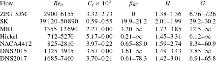
Ranges of common boundary layer parameters for the databases used in the present paper. The ranges cover only the selected regions of each flow, and are expressed in order of streamwise evolution. See text for references.

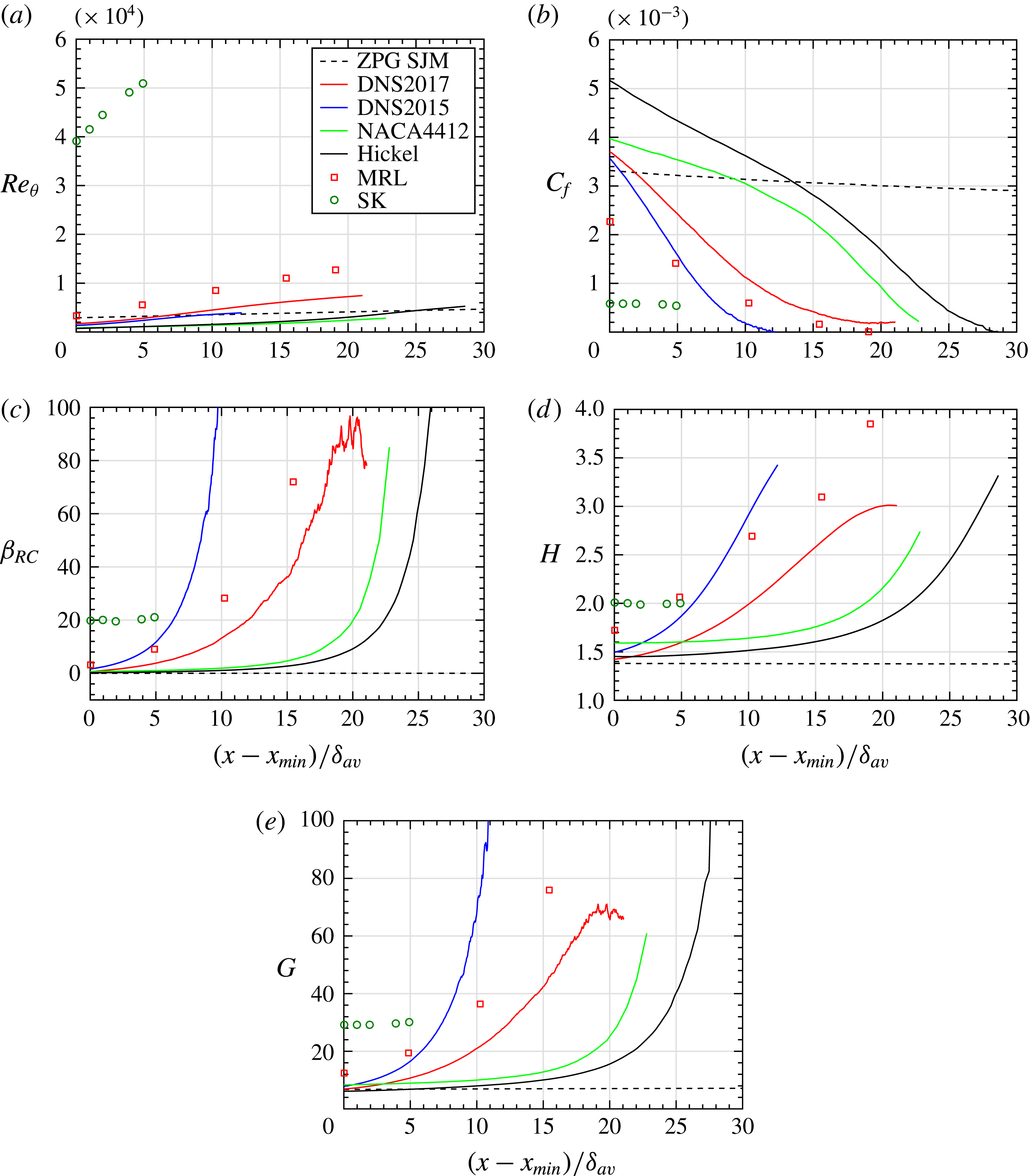
Table 1 presents commonly used boundary layer non-dimensional parameters for these different flows, while figure 1 compares the streamwise evolutions of these parameters. Such a comparison between different APG flows can only be done if $x$ is normalized with a proper reference length $L_{x}$ . Determining such a reference length is not a trivial issue. The theoretical analysis presented in § 4 reveals that one candidate is $L_{x}=(U_{e}/V_{e})\unicode[STIX]{x1D6FF}$ . However, using a reference length that implicitly depends on the variable being normalized, $x$ , is not desirable nor practicable. Furthermore, the normalized variable $x/L_{x}$ would become strongly dependent on the pressure gradient, making the problem circular. For strong pressure gradients, using $L_{x}=(U_{e}/V_{e})\unicode[STIX]{x1D6FF}$ or $L_{x}=\unicode[STIX]{x1D6FF}$ can even lead to the absurd situation where $x/L_{x}$ starts decreasing as $x$ increases. After considering different possibilities, we have determined that a good choice of streamwise reference length is the average value of $\unicode[STIX]{x1D6FF}$ over the $x$ range considered for the given flow, which we name $\unicode[STIX]{x1D6FF}_{av}$ . In other words, $\unicode[STIX]{x1D6FF}_{av}$ is the average size of the boundary layer in the flow region considered. We therefore use in the present paper $L_{x}=\unicode[STIX]{x1D6FF}_{av}$ .

Figure 1.

Streamwise evolution of commonly used boundary layer non-dimensional parameters for the selected regions of the seven flows. Only the first half of the region is shown for ZPG SJM.

To compute the non-dimensional parameters presented in table 1 and figure 1, $U_{e}$ and $\unicode[STIX]{x1D6FF}$ have to be determined first. Note however that the traditional definitions of $U_{e}$ and $\unicode[STIX]{x1D6FF}$ become ill-defined in flows where the external inviscid velocity increases with $y$ . Such a situation is encountered in many flows with curvature or variable divergence of the mean streamlines, such as flows around an airfoil, like NACA4412. A few alternatives have been proposed in the literature to circumvent this problem (Spalart & Watmuff Reference Spalart and Watmuff1993; Vinuesa et al. Reference Vinuesa, Bobke, Örlü and Schlatter2016). In the present study, this situation is encountered for the Hickel flow and in a downstream section of flow NACA4412. In these cases, the wall-normal position of $U_{e}$ is the position where the mean spanwise vorticity levels off to a low value. Such a position is easily detected in these two flows because they were obtained numerically with sufficient spatial resolution. In flows DNS2015 and DNS2017, the external velocity decreases with $y$ . In these cases, $U_{e}$ is defined as the maximum $U$ along $y$ . In all flows, $\unicode[STIX]{x1D6FF}$ is the $y$ position where $U=0.99U_{e}$ , as already mentioned above. It should be kept in mind that, since we are not studying similarity laws, high accuracy in the determination of $\unicode[STIX]{x1D6FF}$ and $U_{e}$ is not required. All integral thicknesses discussed below are obtained by integrating up to $y=\unicode[STIX]{x1D6FF}$ .

In figure 1, the streamwise positions shown for the experimental MRL database cover all available data up to separation. In the case of SK, the five stations are in the quasi-equilibrium range of the flow. For the three simulations performed in rectangular boxes (Hickel, DNS2015, DNS2017), the regions were selected based on two criteria: first point sufficiently far from the inlet plane, and last point at separation or sufficiently far from the outlet plane. In the case of NACA4412, the region selected, on the suction side, is from 0.458 chord from the leading edge (far enough from the transition point at 0.1 chord) up to the trailing edge. Finally, $x_{min}$ is the $x$ coordinate of the first point.

Figure 1(a) presents the distributions of the local boundary layer Reynolds number $Re_{\unicode[STIX]{x1D703}}=U_{e}\unicode[STIX]{x1D703}/\unicode[STIX]{x1D708}$ for the different flows, where $U_{e}$ is the streamwise velocity at the boundary layer edge, $\unicode[STIX]{x1D703}$ is the momentum thickness and $\unicode[STIX]{x1D708}$ is the kinematic viscosity. It can be seen from these distributions of $Re_{\unicode[STIX]{x1D703}}$ that the SK flow is at a much higher Reynolds number than the other flows. In comparison to the ZPG TBL, $Re_{\unicode[STIX]{x1D703}}$ increases more rapidly in the other flows because of the sustained APG. Note however that we show in § 5 that $Re_{\unicode[STIX]{x1D703}}$ should normally represent the local ratio of apparent turbulent forces to viscous forces in the outer region, but that it fails to do it.

Figure 1(b) shows the skin friction coefficient $C_{f}=2\unicode[STIX]{x1D70F}_{w}/(\unicode[STIX]{x1D70C}U_{e}^{2})$ , where $\unicode[STIX]{x1D70F}_{w}$ is the wall shear stress (skin friction) and $\unicode[STIX]{x1D70C}$ is the density. The $C_{f}$ evolutions are quite different for these flows. The initial values of $C_{f}$ depend on the type of upstream effects before $x_{min}$ (pressure gradient, curvature, initial conditions) and on the local Reynolds number. Coefficient $C_{f}$ decreases slowly for the two quasi-equilibrium flows, namely the ZPG TBL and SK flow. The decrease in these cases is mainly due to the increasing Reynolds number (see figure 1 a). In contrast, the $C_{f}$ decrease is important for the non-equilibrium APG TBLs. Three of the flows eventually separate ( $C_{f}=0$ ), whereas NACA4412 and DNS2017 approach separation but never reach it.

In the following discussion, the change from small to large mean velocity defect is expressed with both the shape factor $H=\unicode[STIX]{x1D6FF}^{\ast }/\unicode[STIX]{x1D703}$ , where $\unicode[STIX]{x1D6FF}^{\ast }$ is the displacement thickness, and the Rotta–Clauser pressure-gradient parameter $\unicode[STIX]{x1D6FD}_{RC}$ , which is an outer pressure-gradient parameter:

(2.1) $$\begin{eqnarray}\unicode[STIX]{x1D6FD}_{RC}=\frac{\unicode[STIX]{x1D6FF}^{\ast }}{\unicode[STIX]{x1D70F}_{w}}\frac{\text{d}p_{e}}{\text{d}x}=-\frac{\unicode[STIX]{x1D6E5}}{u_{\unicode[STIX]{x1D70F}}}\frac{\text{d}U_{e}}{\text{d}x}=\left(\frac{U_{po}}{u_{\unicode[STIX]{x1D70F}}}\right)^{2}.\end{eqnarray}$$

Note that the pressure at the edge of the boundary layer $p_{e}$ is used since we are interested here in the outer region. In this manner, we can also express $\unicode[STIX]{x1D6FD}_{RC}$ with the edge velocity gradient as done in the second form shown in (2.1), where $\unicode[STIX]{x1D6E5}$ is a defect displacement thickness defined in table 2, and also known as the Rotta–Clauser length scale (Rotta Reference Rotta1950; Clauser Reference Clauser1954). The last form, $(U_{po}/u_{\unicode[STIX]{x1D70F}})^{2}$ , shows that $\unicode[STIX]{x1D6FD}_{RC}$ is related to the ratio of pertinent outer velocity scales. These velocity scales and the physical significance of $\unicode[STIX]{x1D6FD}_{RC}$ and $H$ are discussed at length in the following sections.

The evolutions of $\unicode[STIX]{x1D6FD}_{RC}$ and $H$ are shown respectively in figures 1(c) and 1(d). Note that $\unicode[STIX]{x1D6FD}_{RC}$ is null in the case of the ZPG TBL and tends to infinity when $u_{\unicode[STIX]{x1D70F}}$ (or $\unicode[STIX]{x1D70F}_{w}$ ) tends to zero, which happens at the downstream end of flows MRL, DNS2015 and Hickel. The values of $C_{f}$ , $\unicode[STIX]{x1D6FD}_{RC}$ and $H$ should be constant for flows with self-similar velocity profiles, i.e. equilibrium TBLs (Rotta Reference Rotta1950; Maciel et al. Reference Maciel, Rossignol and Lemay2006b ). Of the six APG TBLs considered here, the only one that approaches such a condition is SK, which was designed to be an equilibrium TBL. 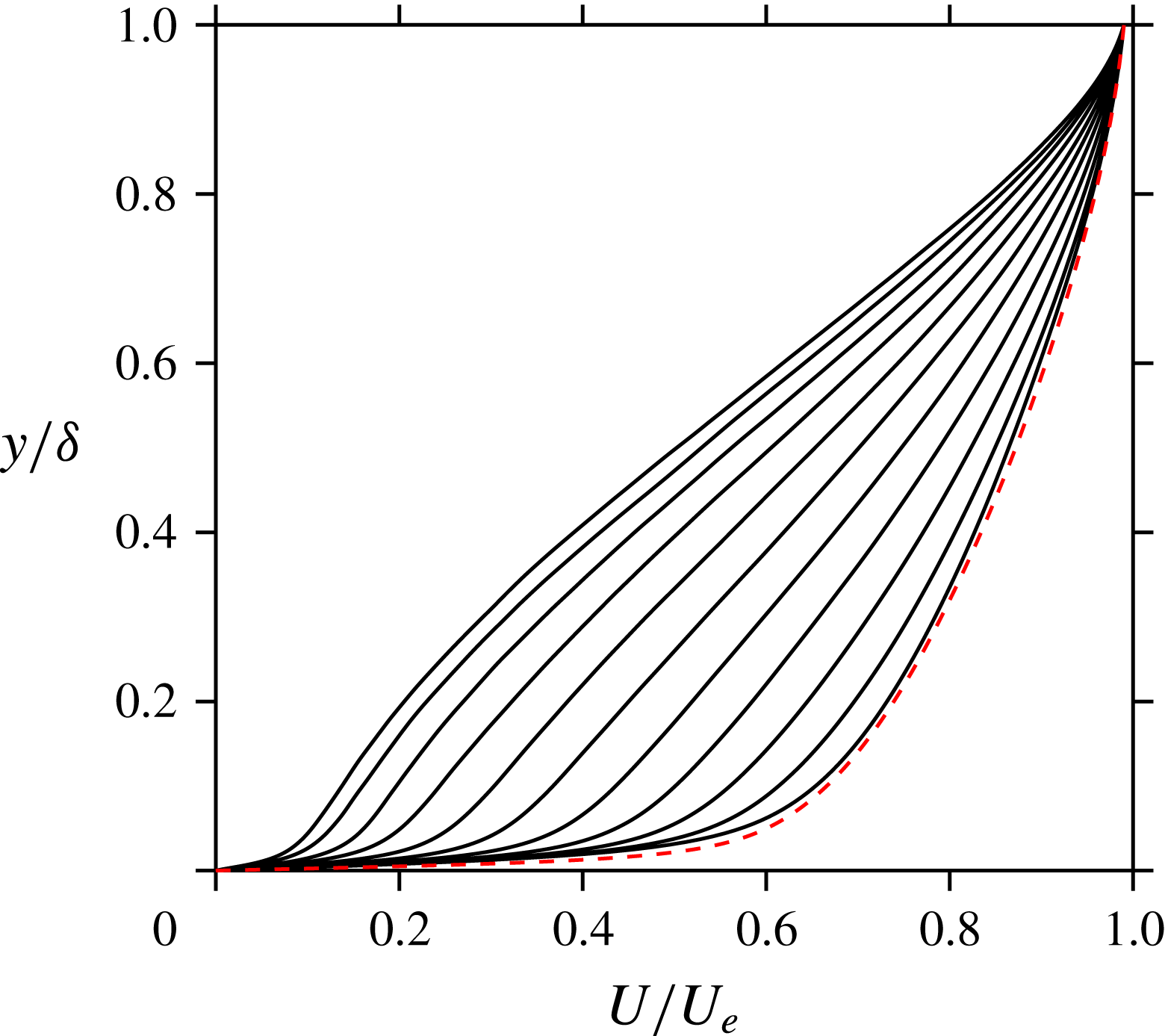The other five APG TBLs exhibit steady increases of $\unicode[STIX]{x1D6FD}_{RC}$ and $H$ in the flow zones considered, except for the beginning of Hickel and the end of DNS2017. These increases indicate that these are disequilibrium TBLs with increasing momentum defect. The mean velocity profiles of figure 2 show the increase of momentum defect in the case of DNS2017. The trend is qualitatively similar for the other four non-equilibrium APG TBLs. All five non-equilibrium APG TBLs present regions of rapid increase of $\unicode[STIX]{x1D6FD}_{RC}$ and $H$ . They can all be considered as flows with strong disequilibrium conditions.

Table 2.

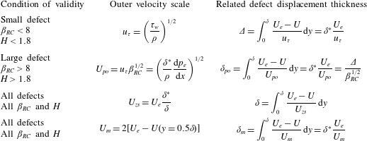
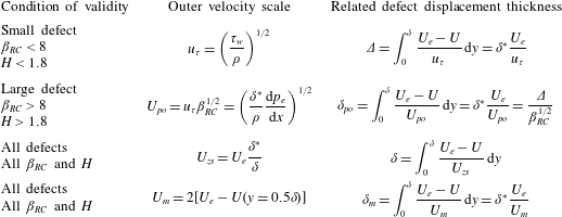
Velocity and length scales for the outer region. The conditions of validity expressed in terms of inequalities are for the scaling of the Reynolds stresses only, and they are approximate since they depend on Reynolds number and upstream history.

Figure 2.

Equidistant mean velocity profiles of DNS2017 spanning the selected streamwise region shown in figure 1 (solid lines), and of ZPG SJM at $Re_{\unicode[STIX]{x1D703}}=2900$ (dashed red line).

We also present in figure 1(e) the defect shape factor

(2.2) $$\begin{eqnarray}G=\int _{0}^{\unicode[STIX]{x1D6FF}}\left(\frac{U_{e}-U}{u_{\unicode[STIX]{x1D70F}}}\right)^{2}\,\text{d}y\bigg/\int _{0}^{\unicode[STIX]{x1D6FF}}\frac{U_{e}-U}{u_{\unicode[STIX]{x1D70F}}}\,\text{d}y=\frac{U_{e}}{u_{\unicode[STIX]{x1D70F}}}\left[1-\frac{1}{H}\right].\end{eqnarray}$$

This was introduced by Rotta (Reference Rotta1950) to analyse TBLs in arbitrary pressure distributions and four years later by Clauser (Reference Clauser1954) in his study of equilibrium APG TBLs. Like $H$ and $\unicode[STIX]{x1D6FD}_{RC}$ , $G$ increases with increasing velocity defect. According to Clauser (Reference Clauser1954) and Mellor & Gibson (Reference Mellor and Gibson1966), $G$ is less dependent on the Reynolds number (or $u_{\unicode[STIX]{x1D70F}}/U_{e}$ ) than $H$ in the case of equilibrium TBLs. However, as opposed to $H$ but similarly to $\unicode[STIX]{x1D6FD}_{RC}$ , $G$ does not remain finite at separation or reattachment, when $u_{\unicode[STIX]{x1D70F}}$ is zero. This is the reason why the last portions of flows MRL, DNS2015 and Hickel do not appear in figure 1(e).

3 Velocity and length scales of the outer region

We demonstrate in this section that the velocity and length scales shown in table 2 are pertinent scales for the mean velocity defect and the Reynolds stresses in the outer region of APG TBLs. We also determine under what precise conditions they can be considered proper scales, since some scales are restricted to small-defect TBLs ( $u_{\unicode[STIX]{x1D70F}}$ , $\unicode[STIX]{x1D6E5}$ ) or large-defect TBLs ( $U_{po}$ , $\unicode[STIX]{x1D6FF}_{po}$ ), while the others are proper scales for all velocity-defect conditions ( $U_{zs}$ , $\unicode[STIX]{x1D6FF}$ ; $U_{m}$ , $\unicode[STIX]{x1D6FF}_{m}$ ). It is important to stress that the scales studied here are not the only ones possible. They have been chosen because they are theoretically valid and this validity has been confirmed in the past with solid empirical evidence.

As stated at the end of the introduction, there is no precise definition of the outer region in the case of large-defect APG TBLs. In this study, the lower limit of the outer region is taken as the approximate height where the viscous stress gradient is negligible with respect to the Reynolds shear stress gradient. For the flows studied here, this lower limit corresponds approximately to $y=0.15\unicode[STIX]{x1D6FF}$ .

Since the velocity scales presented in table 2 are scales of the mean velocity defect in the outer region, it is logical to use the corresponding defect displacement thickness as the length scale. These are indeed the outer length scales shown in table 2. The advantage of defect displacement thicknesses is that they are independent of Reynolds number and roughness in the case of equilibrium TBLs (Clauser Reference Clauser1954), which is also the case of $\unicode[STIX]{x1D6FF}$ (since it is also a defect displacement thickness, as seen in table 2) but not of $\unicode[STIX]{x1D6FF}^{\ast }$ and $\unicode[STIX]{x1D703}$ . In the case of equilibrium TBLs, it is easy to show that $\unicode[STIX]{x1D6FF}^{\ast }/\unicode[STIX]{x1D6FF}$ and $\unicode[STIX]{x1D703}/\unicode[STIX]{x1D6FF}$ tend to zero like $C_{f}^{1/2}$ ( $u_{\unicode[STIX]{x1D70F}}/U_{e}$ ) as the Reynolds number tends to infinity. Therefore, $\unicode[STIX]{x1D6FF}^{\ast }$ and $\unicode[STIX]{x1D703}$ are not appropriate outer length scales.

However, there is no obligation to stick to the pairs shown in table 2, firstly, because the velocity scales scale not only the mean velocity defect but also the Reynolds stresses, and secondly, because what matters is that the length scale follows the magnitude change of the outer region thickness under all conditions. In the following, we generally use the boundary layer thickness $\unicode[STIX]{x1D6FF}$ as the outer length scale because it simplifies the analysis of the data.

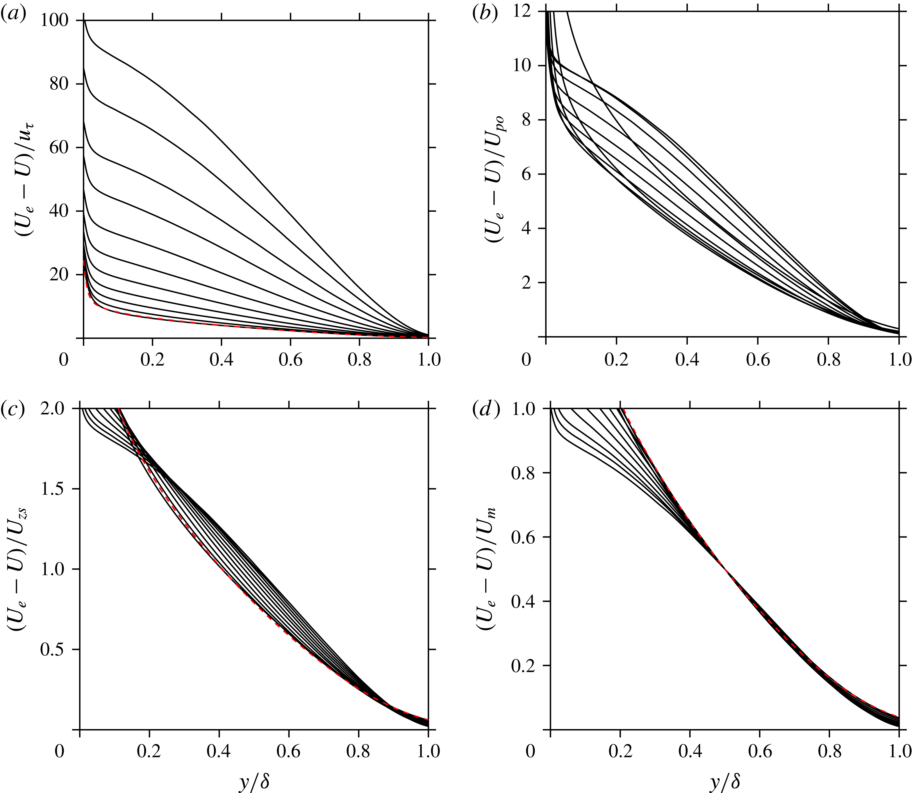
Figure 3 shows the mean velocity defect normalized by the four velocity scales presented in table 2 in the case of the flow DNS2017 and the ZPG TBL of SJM. The same positions as in figure 2 are used. The trends seen in figure 3 as the velocity defect increases are qualitatively similar for the four other non-equilibrium APG TBLs. It is important to mention that in the case of non-equilibrium APG TBLs, we do not expect to find self-similar behaviour in the outer region or, even less, a universal outer behaviour common to all non-equilibrium flows. Therefore, in the context of non-equilibrium APG TBLs, a scale should always reflect the order of magnitude of the scaled variable, but it is not required that it reveals scale invariance – that it ‘collapses profiles’ of the scaled variable. The four plots of figure 3 clearly show that such a collapse is not possible. No velocity scale will be able to reveal self-similarity or universal similarity since the shape of the mean velocity-defect profile in the outer region varies as a function of local conditions and upstream history. Self-similarity of the mean velocity-defect profile in the outer region is expected only in the case of equilibrium TBLs (Rotta Reference Rotta1950; Clauser Reference Clauser1954), which can only be truly achieved when approaching an infinite Reynolds number (Rotta Reference Rotta1950; Maciel et al. Reference Maciel, Rossignol and Lemay2006b ).

Figure 3.

Mean velocity-defect profiles for the same 11 positions of DNS2017 as in figure 2 (solid lines) and for ZPG SJM at $Re_{\unicode[STIX]{x1D703}}=2900$ (dashed red line). Normalized with (a) $u_{\unicode[STIX]{x1D70F}}$ , (b) $U_{po}$ , (c) $U_{zs}$ and (d) $U_{m}$ .

The friction velocity $u_{\unicode[STIX]{x1D70F}}$ is the outer velocity scale generally used for canonical wall flows (ZPG TBL, pipe and channel flows) and for small-defect pressure-gradient TBLs (both favourable- and adverse-pressure-gradient cases). In the latter case, the outer length scale used in combination with $u_{\unicode[STIX]{x1D70F}}$ is usually $\unicode[STIX]{x1D6FF}$ or $\unicode[STIX]{x1D6E5}$ . For large mean velocity defect (large $\unicode[STIX]{x1D6FD}_{RC}$ and $H$ ), it is known that $u_{\unicode[STIX]{x1D70F}}$ and $\unicode[STIX]{x1D6E5}$ are no longer proper outer scales. Figure 3(a) illustrates this point for $u_{\unicode[STIX]{x1D70F}}$ . The mean velocity defect normalized with $u_{\unicode[STIX]{x1D70F}}$ increases by one order of magnitude with a change of shape factor $H$ from 1.4 to 3.0. The situation is even worse for flows that separate, such as MRL, DNS2015 and Hickel, since the mean velocity defect normalized with $u_{\unicode[STIX]{x1D70F}}$ tends to infinity at separation. Nonetheless, the five non-equilibrium TBLs studied here indicate that $u_{\unicode[STIX]{x1D70F}}$ can be considered a scale of the mean velocity defect up to about $H=1.8$ . In the case of the DNS2017 profiles shown in figure 3(a), this corresponds to the five lower profiles. For $H<1.8$ , the order of magnitude of the mean velocity defect normalized with $u_{\unicode[STIX]{x1D70F}}$ is 10 for all TBLs.

For large mean velocity-defect TBLs, Mellor & Gibson (Reference Mellor and Gibson1966) proposed $U_{po}$ and $\unicode[STIX]{x1D6FF}_{po}$ , where the index $p$ stands for pressure and $o$ for outer region. As can be seen with the equations in table 2, these scales were obtained directly by a transformation of the traditional scales for small $\unicode[STIX]{x1D6FD}_{RC}$ , namely $u_{\unicode[STIX]{x1D70F}}$ and $\unicode[STIX]{x1D6E5}$ , by using the factor $\unicode[STIX]{x1D6FD}_{RC}^{1/2}$ . Figure 3(b) shows that $U_{po}$ can scale all the mean velocity-defect profiles of DNS2017, with an order of magnitude of 10, and this is also the case for all the other APG TBLs. However, $U_{po}$ cannot be used for ZPG TBLs since it is null in this case. It cannot be used either for cases or flow regions where $\text{d}p_{e}/\text{d}x$ is close to zero.

Figures 3(c) and 3(d) show that the Zagarola–Smits velocity scale $U_{zs}$ and the mixing-layer-type velocity scale $U_{m}$ scale the mean velocity defect in all defect conditions, leading to an order of magnitude of one of the scaled defect. This has already been demonstrated in the past by Maciel et al. (Reference Maciel, Rossignol and Lemay2006b ) and Logdberg, Angele & Alfredsson (Reference Logdberg, Angele and Alfredsson2008) in the case of $U_{zs}$ and by Gungor et al. (Reference Gungor, Maciel, Simens and Soria2014) and Gungor et al. (Reference Gungor, Maciel, Simens and Soria2016) in the case of $U_{m}$ . Gungor et al. (Reference Gungor, Maciel, Simens and Soria2014) introduced $U_{m}$ in order to be able to compare the velocity statistics of APG TBLs with those of mixing layers. Indeed, $U_{m}$ is a velocity scale of the type used for mixing layers.

Although some readers might be tempted to see ‘collapse of the profiles’ in the case of $U_{m}$ , it is not the case, and it is not the case for any of the other non-equilibrium APG TBLs. We emphasize that $U_{m}$ is not a ‘better’ outer velocity scale for the mean velocity defect than the others, since self-similarity or general scale invariance does not exist for non-equilibrium TBLs. Conversely, in the case of equilibrium APG TBLs, all the velocity scales of table 2 reveal self-similarity of the mean velocity-defect profile, except $u_{\unicode[STIX]{x1D70F}}$ at separation and reattachment and $U_{po}$ for ZPG TBLs. This is simply because equilibrium APG TBLs are by definition in dynamic equilibrium in the outer region, and this dynamic equilibrium does not depend on any scale.

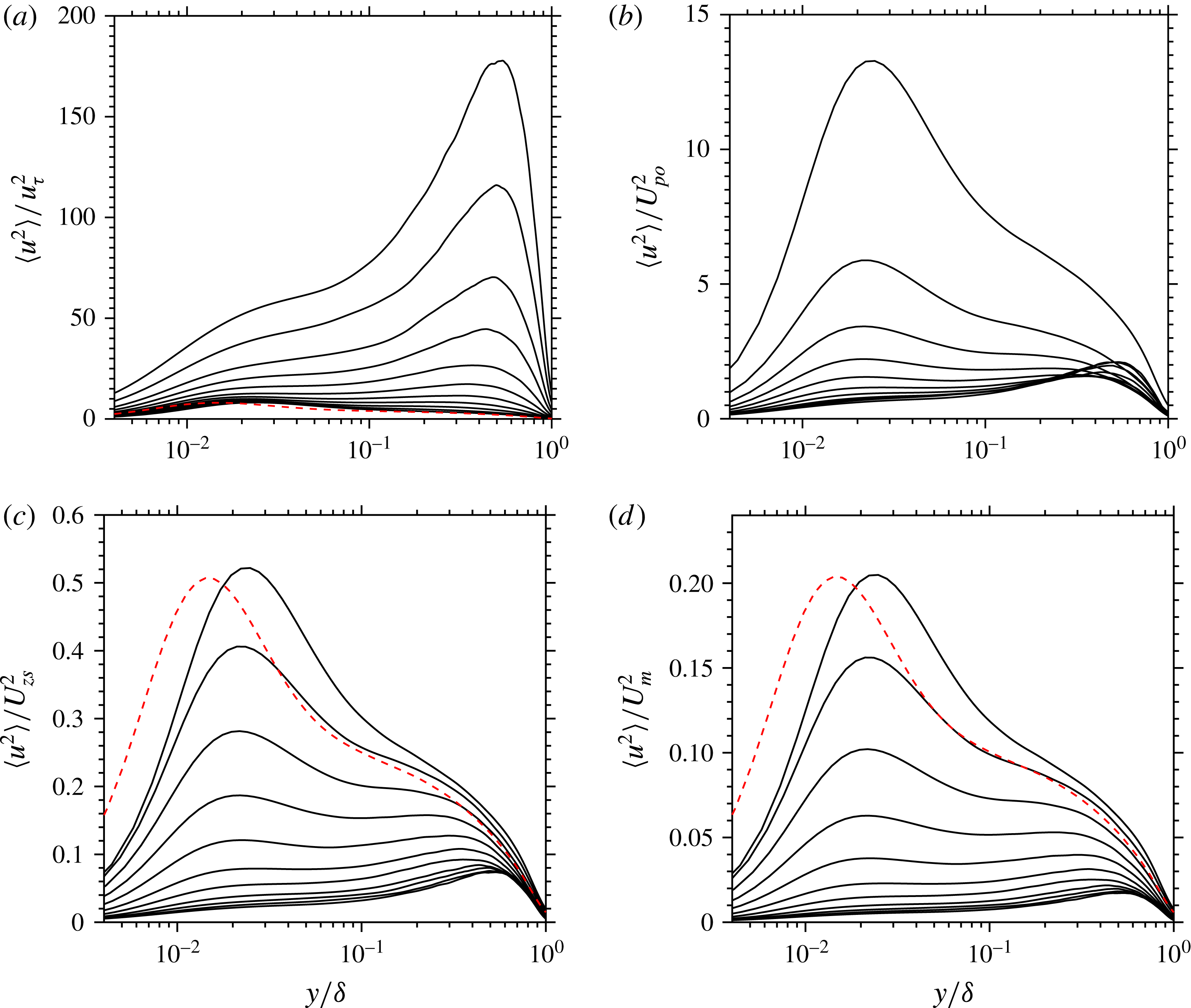
We now consider the outer scaling of the Reynolds stresses. Figure 4 shows $\langle u^{2}\rangle$ normalized by the four velocity scales presented in table 2, for the same positions of DNS2017 and ZPG SJM as in figure 3. The abscissa has a logarithmic scale in order to reveal the near-wall behaviour. The scaling situation is similar to what was discussed for the mean velocity defect: $u_{\unicode[STIX]{x1D70F}}$ scales $\langle u^{2}\rangle$ only in the small-defect cases while the other three velocity scales work for all defect cases, except $U_{po}$ , which cannot be used for cases where $\text{d}p_{e}/\text{d}x$ is zero or close to zero. The disappearance of the near-wall peak and the appearance of an outer peak as the defect increases can clearly be seen in all the plots of figure 4. The difference in position of the near-wall peaks of the ZPG TBL and of the first profile of DNS2017 is a Reynolds-number effect due to the fact that the outer length scale $\unicode[STIX]{x1D6FF}$ is used in these figures.

Figure 4.

Semilog plots of $\langle u^{2}\rangle$ for the same 11 positions of DNS2017 as in figure 2 (solid lines) and for ZPG SJM at $Re_{\unicode[STIX]{x1D703}}=2900$ (dashed red line). Normalized with (a) $u_{\unicode[STIX]{x1D70F}}$ , (b) $U_{po}$ , (c) $U_{zs}$ and (d) $U_{m}$ . Note that $U_{po}=0$ for ZPG TBLs.

The evolution of the scaled $\langle u^{2}\rangle$ profiles with $H$ seen in figure 4 is qualitatively similar for the other four non-equilibrium APG TBLs. This observation is also true for the scaled profiles of the other components of the Reynolds stress tensor (see figures 5–9). For a given $H$ value, the presence of one or two peaks in the $\langle u^{2}\rangle$ profiles, the position of the outer peak (when it exists), and the amplitude of the scaled peaks is similar for all APG TBLs, including the quasi-equilibrium one of SK. This will be shown below.

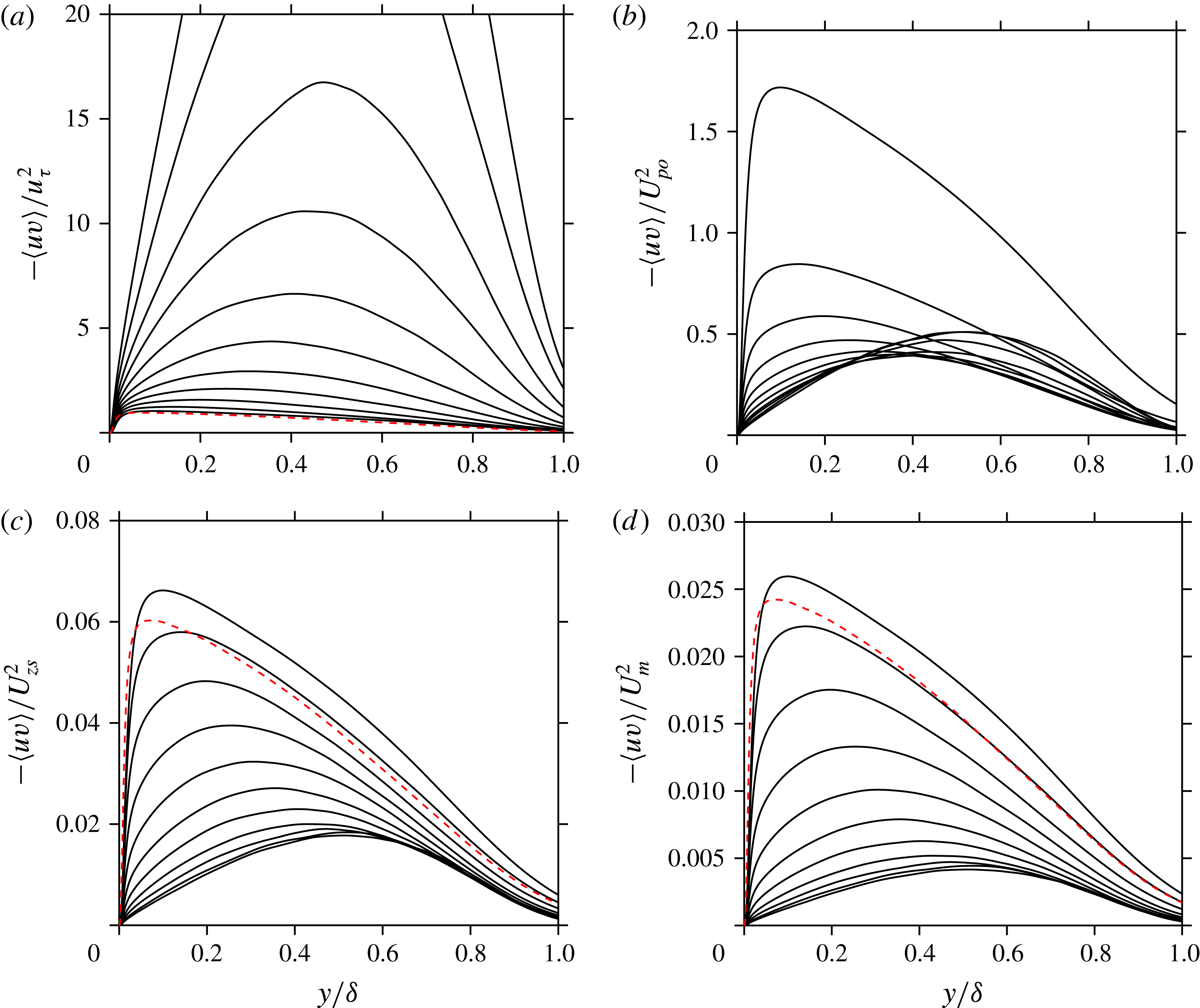
Figure 5 shows the Reynolds shear stress normalized by the four velocity scales, again for the same positions of DNS2017 and ZPG SJM as in figure 3. The Reynolds shear stress profiles, like those of $\langle v^{2}\rangle$ , have always only one maximum, as opposed to $\langle u^{2}\rangle$ and $\langle w^{2}\rangle$ , whose near-wall maximum is distinct from the outer maximum. The maximum of the Reynolds shear stress moves away from the wall as $H$ increases. As expected, it can be seen that $u_{\unicode[STIX]{x1D70F}}$ scales the Reynolds shear stress only when the velocity defect is small, while $U_{po}$ scales it when the defect is large. When the scaling is valid, $-\langle uv\rangle /u_{\unicode[STIX]{x1D70F}}^{2}$ and $-\langle uv\rangle /U_{po}^{2}$ are of order of magnitude one. In contrast, for all types of TBLs, $-\langle uv\rangle /U_{zs}^{2}$ and $-\langle uv\rangle /U_{m}^{2}$ are of order of magnitude 0.1 and 0.01, respectively. We find the same orders of magnitude for all the flows studied here. The order of magnitude of the scaled Reynolds shear stress is an important result for the analysis of the next section.

Figure 5.

Reynolds shear stress for the same 11 positions of DNS2017 as in figure 2 (solid lines) and for ZPG SJM at $Re_{\unicode[STIX]{x1D703}}=2900$ (dashed red line). Normalized with (a) $u_{\unicode[STIX]{x1D70F}}$ , (b) $U_{po}$ , (c) $U_{zs}$ and (d) $U_{m}$ . Note that $U_{po}=0$ for ZPG TBLs.

As an aside, it is interesting to note that Abe (Reference Abe2017) has found that the maximum Reynolds shear stress scales very well the root-mean-square value of the wall-pressure fluctuations throughout the APG zone and at the beginning of the separated zone in the case of turbulent separation bubbles. Wall-pressure fluctuations can therefore be strongly related to outer region motions.

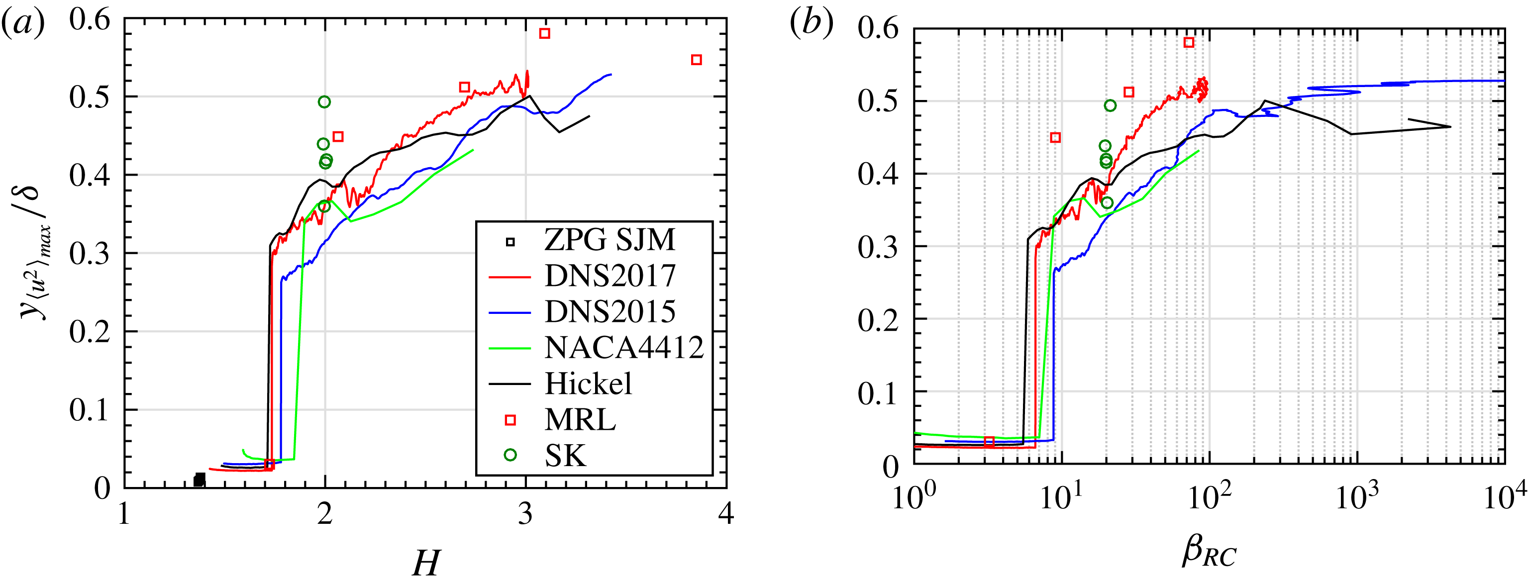
The maxima of the Reynolds stress profiles will be used to demonstrate the scaling behaviour of all Reynolds stress components and for all flows. Beforehand, figure 6 shows how the wall-normal position of this maximum evolves as a function of $H$ and $\unicode[STIX]{x1D6FD}_{RC}$ , in the case of $\langle u^{2}\rangle$ . Although not unique, it is seen that the evolution of the wall-normal position is quite similar for all the flows. Firstly, the transition from a near-wall-peak maximum to an outer-peak maximum occurs in the range $H=1.7$ –1.9 ( $\unicode[STIX]{x1D6FD}_{RC}=5$ –9). The wall-normal position of the outer-peak maximum then increases steadily and levels off around $0.5\unicode[STIX]{x1D6FF}$ for large $H$ (large $\unicode[STIX]{x1D6FD}_{RC}$ ). Because $\unicode[STIX]{x1D6FD}_{RC}$ varies from zero to infinity, it is not a practical indicator of the state of the boundary layer. This is seen in figure 6(b) where flows or flow regions with null or small $\text{d}p_{e}/\text{d}x$ ( $\unicode[STIX]{x1D6FD}_{RC}<1$ ) and close to separation (null or small $u_{\unicode[STIX]{x1D70F}}$ ; $\unicode[STIX]{x1D6FD}_{RC}>10^{4}$ ) cannot be shown. From now on, we will use only $H$ as an indicator of the extent of the mean velocity defect since it allows data near or at ZPG and near or at separation or reattachment to be shown.

Figure 6.

Wall-normal position of the maximum of $\langle u^{2}\rangle$ as a function of (a) $H$ and (b) $\unicode[STIX]{x1D6FD}_{RC}$ .

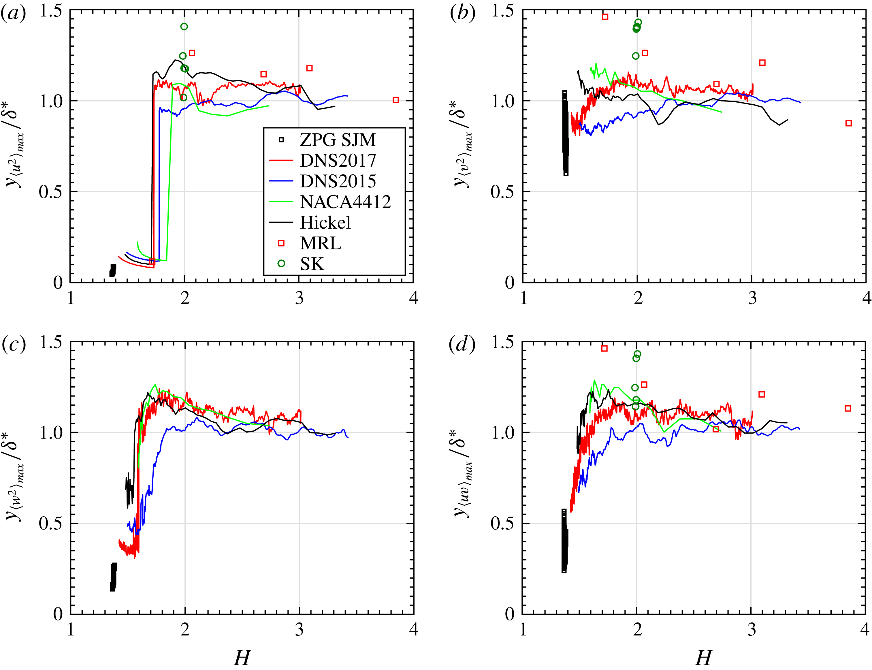
Figure 7 shows the wall-normal position of the maximum of all Reynolds stress components as a function of $H$ . In this figure, the wall-normal position is normalized by $\unicode[STIX]{x1D6FF}^{\ast }$ to show that $\unicode[STIX]{x1D6FF}^{\ast }$ indeed scales the position of the outer maximum of all Reynolds stresses (similar location for the four Reynolds stresses) for all flows and all defect cases when such an outer maximum exists. Kitsios et al. (Reference Kitsios, Sekimoto, Atkinson, Sillero, Borrell, Gungor, Jimnez and Soria2017) also noticed that the outer peak of all Reynolds stresses was located at $y=\unicode[STIX]{x1D6FF}^{\ast }$ in the case of a near-equilibrium APG TBL with $H=2.35$ . In the large-defect cases of the present flows, the outer peaks are in fact close to the position of the outermost inflection point of the mean velocity profile, as observed previously by Elsberry, Zhou & Wygnanski (Reference Elsberry, Loeffler, Zhou and Wygnanski2000) in a quasi-equilibrium large-defect APG TBL with $H\approx 2.45$ . These authors suggested that their flow was dominated by a single inflectional instability occurring at the position of the outermost inflection point of the mean velocity profile. In the present five non-equilibrium APG TBLs, there are however upstream flow regions with smaller mean velocity defects (roughly for $H<2$ ) where the Reynolds stresses have an outer maximum while the mean velocity profile does not have an inflection point. Furthermore, in the case of flow DNS2015, Maciel, Gungor & Simens (Reference Maciel, Gungor and Simens2017) studied the coherent structures in the outer region of the large-defect part of the flow and they were not able to detect any sign of an inflectional instability. The presence or not of an inflectional instability for large-defect TBLs is still an open issue.

Figure 7.

Wall-normal position of the maximum of the Reynolds stress components, normalized by $\unicode[STIX]{x1D6FF}^{\ast }$ , as a function of $H$ .

In the case of $\langle u^{2}\rangle$ and $\langle w^{2}\rangle$ (figure 7 a,c), the abrupt rise of the maximum position as $H$ increases corresponds to a switch from a near-wall to an outer maximum, which is the position in the flow where the outer maximum now exceeds the near-wall maximum. Interestingly, for all flows for which such a switch can be followed (the numerical ones), the switch does not occur for the same $H$ value for $\langle u^{2}\rangle$ and $\langle w^{2}\rangle$ . It occurs at a smaller $H$ for $\langle w^{2}\rangle$ than for $\langle u^{2}\rangle$ . In other words, the stronger near-wall peak of $\langle u^{2}\rangle$ takes more time to decay than the near-wall peak of $\langle w^{2}\rangle$ in the decelerating non-equilibrium TBLs.

In the case of $\langle v^{2}\rangle$ and $\langle uv\rangle$ , the smoother evolutions seen in figure 7(b,d) reflect the fact that the profiles of these Reynolds stresses always have only one maximum at a time (see for instance figure 5), as opposed to $\langle u^{2}\rangle$ and $\langle w^{2}\rangle$ whose near-wall maximum is distinct from the outer maximum (see figure 4).

The fact that $\unicode[STIX]{x1D6FF}^{\ast }$ scales the position of the outer maximum of the Reynolds stresses raises an interesting issue. If it remains the case for higher Reynolds numbers, then these outer peaks would very slowly approach the wall as the Reynolds number increases since, as mentioned previously, $\unicode[STIX]{x1D6FF}^{\ast }/\unicode[STIX]{x1D6FF}$ slowly tends to zero as the Reynolds number tends to infinity. Furthermore, in connection with what has just been said, it is also worth mentioning that the fact that $\unicode[STIX]{x1D6FF}^{\ast }$ scales the position of the outer maximum of the Reynolds stresses does not mean that $\unicode[STIX]{x1D6FF}^{\ast }$ is the proper length scale to characterize the size of the outer region.

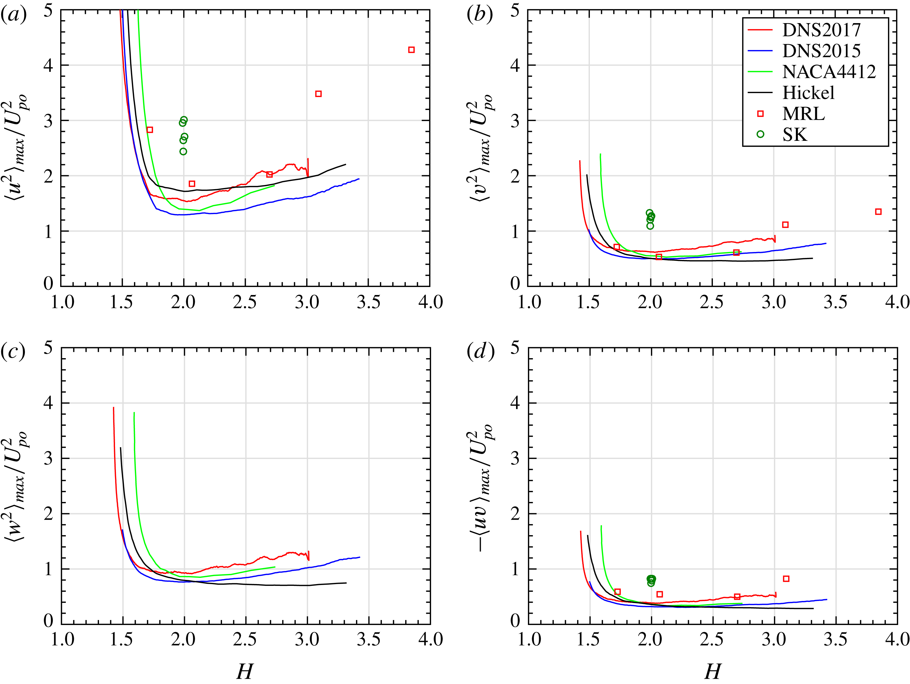
Now that the behaviours of the maxima of the Reynolds stresses have been assessed, these maxima can be used to demonstrate the scaling behaviour of all Reynolds stress components and for all flows. Figure 8 shows how the maximum value of the Reynolds stresses normalized with $U_{po}^{2}$ evolves with mean velocity defect (note that ZPG TBL data cannot be shown with $U_{po}$ as a scale). It can be seen that $U_{po}$ is indeed a scale of the Reynolds stresses for large-defect TBLs, ‘large’ corresponding to approximately $H>1.8$ . The scaled Reynolds stresses are of order of magnitude one. The scaled outer peaks slightly increase with $H$ for all non-equilibrium TBLs, with the exception of Hickel’s flow. Similar plots for the maximum value of the Reynolds stresses normalized with $u_{\unicode[STIX]{x1D70F}}^{2}$ (not shown) reveal of course an inverse trend, in the sense that $u_{\unicode[STIX]{x1D70F}}$ is a scale of the Reynolds stresses only for small-defect TBLs, approximately for $H<1.8$ .

Figure 8.

Maximum value of the Reynolds stresses normalized with $U_{po}^{2}$ . Note that $U_{po}=0$ for ZPG TBLs.

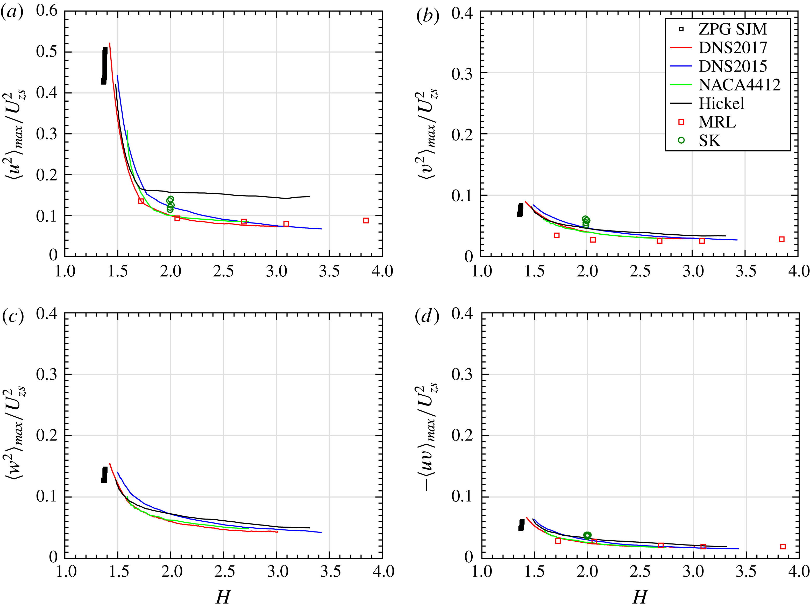
The maximum value of the Reynolds stresses normalized with $U_{zs}^{2}$ are presented in figure 9, where it is now possible to include also the ZPG TBL data. This figure shows that $U_{zs}$ is a scale of all Reynolds stresses for all TBLs, whatever the extent of the mean velocity defect. The Reynolds stresses scaled with $U_{zs}^{2}$ are of order of magnitude 0.1. The initial sharp decrease of the maximum of $\langle u^{2}\rangle$ seen in figure 9(a) corresponds to the attenuation of the near-wall peak as $H$ increases, but the near-wall peak is still higher than the outer peak in this range of low $H$ values. As seen previously with figure 6, once $H$ exceeds approximately 1.8, the maximum of $\langle u^{2}\rangle$ corresponds now to the outer peak. For all Reynolds stresses, the value of the outer peak scaled with $U_{zs}^{2}$ slightly decreases with $H$ in the five non-equilibrium flows. In the case of the two quasi-equilibrium TBLs, namely the ZPG TBL and SK flow, the maximum of the Reynolds stresses scaled with $U_{zs}^{2}$ decreases with Reynolds number. The only exception is $\langle -uv\rangle _{max}/U_{zs}^{2}$ of SK, which remains fairly constant. The behaviour of the Reynolds stresses scaled with $U_{m}^{2}$ is very similar to that of the Reynolds stresses scaled with $U_{zs}^{2}$ for all flows. This can be appreciated with figures 4(c,d) and 5(c,d) for flow DNS2017.

Figure 9.

Maximum value of the Reynolds stresses normalized with $U_{zs}^{2}$ .

4 Consistent set of non-dimensional parameters

Now that the behaviour of the outer length and velocity scales is known, the incompressible, two-dimensional and Reynolds-averaged TBL equations are used to bring out in a consistent manner the non-dimensional parameters characterizing the outer region of APG TBLs. These equations are

(4.1) $$\begin{eqnarray}\displaystyle & \displaystyle \frac{\unicode[STIX]{x2202}U}{\unicode[STIX]{x2202}x}+\frac{\unicode[STIX]{x2202}V}{\unicode[STIX]{x2202}y}=0, & \displaystyle\end{eqnarray}$$

(4.2) $$\begin{eqnarray}\displaystyle & \displaystyle 0=-U\frac{\unicode[STIX]{x2202}U}{\unicode[STIX]{x2202}x}-V\frac{\unicode[STIX]{x2202}U}{\unicode[STIX]{x2202}y}-\frac{1}{\unicode[STIX]{x1D70C}}\frac{\text{d}p_{e}}{\text{d}x}-\frac{\unicode[STIX]{x2202}\langle uv\rangle }{\unicode[STIX]{x2202}y}-\frac{\unicode[STIX]{x2202}(\langle u^{2}\rangle -\langle v^{2}\rangle )}{\unicode[STIX]{x2202}x}+\unicode[STIX]{x1D708}\frac{\unicode[STIX]{x2202}^{2}U}{\unicode[STIX]{x2202}y^{2}}, & \displaystyle\end{eqnarray}$$

where the pressure gradient is taken at the edge of the boundary layer (index $e$ ). The momentum equation (4.2) is written in the format of a force balance. Equations (4.1) and (4.2) are now transformed into a single equation of motion with the following two steps. Firstly, $\unicode[STIX]{x2202}U/\unicode[STIX]{x2202}x$ in the streamwise momentum equation (4.2) is replaced by $-\unicode[STIX]{x2202}V/\unicode[STIX]{x2202}y$ from the continuity equation (4.1). Secondly, the Reynolds normal stress gradients are neglected. They are non-negligible, but small, only for very large-defect TBLs, typically very close to separation. Performing the aforementioned combination and simplification, the TBL equations are reduced to a single partial differential equation, (4.3), with no streamwise derivatives for the velocity moments – a crucial point for the analysis:

(4.3) $$\begin{eqnarray}0=U\frac{\unicode[STIX]{x2202}V}{\unicode[STIX]{x2202}y}-V\frac{\unicode[STIX]{x2202}U}{\unicode[STIX]{x2202}y}-\frac{1}{\unicode[STIX]{x1D70C}}\frac{\text{d}p_{e}}{\text{d}x}-\frac{\unicode[STIX]{x2202}\langle uv\rangle }{\unicode[STIX]{x2202}y}+\unicode[STIX]{x1D708}\frac{\unicode[STIX]{x2202}^{2}U}{\unicode[STIX]{x2202}y^{2}}.\end{eqnarray}$$

The non-dimensional variables are chosen as

(4.4a,b ) $$\begin{eqnarray}\unicode[STIX]{x1D702}(x,y)=\frac{y}{L_{o}},\quad x^{\ast }(x,y)=\frac{x}{L_{x}},\end{eqnarray}$$

(4.5a-c ) $$\begin{eqnarray}U^{\ast }(x^{\ast },\unicode[STIX]{x1D702})=\frac{U}{U_{e}},\quad V^{\ast }(x^{\ast },\unicode[STIX]{x1D702})=\frac{V}{V_{e}},\quad R_{12}^{\ast }(x^{\ast },\unicode[STIX]{x1D702})=-\frac{\langle uv\rangle }{U_{o}^{2}},\end{eqnarray}$$

where generic wall-normal length scale $L_{o}$ and velocity scale $U_{o}$ of the outer region are used, for the moment, in order to retain generality.

The above non-dimensional variables have been chosen with care in order to obtain physically meaningful non-dimensional parameters. This choice deserves to be explained. Firstly, the reference velocities $U_{e}$ , $V_{e}$ and $U_{o}$ ensure that each term in the resulting non-dimensional equation of motion (4.11) is of known order of magnitude. The resulting non-dimensional variables are normalized variables in the case of $\unicode[STIX]{x1D702}$ , $x^{\ast }$ , $U^{\ast }$ and $V^{\ast }$ ( $\unicode[STIX]{x1D702}$ , $U^{\ast }$ and $V^{\ast }$ are bounded between zero and one in the outer region), whereas $R_{12}^{\ast }$ is a scaled variable, in the sense that it retains the same order of magnitude throughout the flow regions considered. However, the constant order of magnitude of the scaled variable $R_{12}^{\ast }$ is not necessarily one. As we saw in the previous section (see figures 5, 8 and 9), results show that $-\langle uv\rangle /u_{\unicode[STIX]{x1D70F}}^{2}$ and $-\langle uv\rangle /U_{po}^{2}$ are of order of magnitude one in their domains of validity, roughly $H<1.8$ and $H>1.8$ , respectively. In contrast, $-\langle uv\rangle /U_{zs}^{2}$ and $-\langle uv\rangle /U_{m}^{2}$ are respectively of order of magnitude 0.1 and 0.01 for all types of TBL. The fact that the order of magnitude is not one in the case of $U_{zs}$ and $U_{m}$ has an impact on the interpretation of the non-dimensional parameters derived below, as we will see in the next section.

Secondly, by using the normalization $U^{\ast }=U/U_{e}$ instead of the defect formulation (scaled mean velocity defect)

(4.6) $$\begin{eqnarray}\frac{U_{e}-U}{U_{o}},\end{eqnarray}$$

we ensure that the pressure force will not be mixed with other forces in the resulting non-dimensional equation of motion – this is a drawback of all defect formulations of the boundary layer equations, such as the equation of motion of equilibrium boundary layers and the momentum integral equation. In this manner, the resulting non-dimensional parameters will have a clear physical meaning. The normalization $U^{\ast }=U/U_{e}$ is nonetheless fully consistent with the mean velocity-defect scaling (4.6). This can be demonstrated with matched asymptotic expansions (Afzal Reference Afzal1983, Reference Afzal2008; Panton Reference Panton2005), where the outer expansion is also usually expressed as $U/U_{e}$ . In the present representation, assuming a fixed $x^{\ast }$ , we can write the outer expansion as

(4.7) $$\begin{eqnarray}U^{\ast }(x^{\ast },\unicode[STIX]{x1D702})=\frac{U}{U_{e}}=1+\unicode[STIX]{x1D6FE}F_{1}(x^{\ast },\unicode[STIX]{x1D702})+\cdots \,,\end{eqnarray}$$

where $F_{1}$ is the first-order function. By choosing $\unicode[STIX]{x1D6FE}=U_{o}/U_{e}$ as the perturbation parameter or gauge function in the outer expansion of $U^{\ast }$ , the first-order function $F_{1}$ is, to first order, the scaled velocity defect:

(4.8) $$\begin{eqnarray}-F_{1}(x^{\ast },\unicode[STIX]{x1D702})\approx \frac{1}{\unicode[STIX]{x1D6FE}}(1-U^{\ast })=\frac{U_{e}-U}{U_{o}}.\end{eqnarray}$$

The scale of the velocity defect is therefore $U_{o}$ , not $U_{e}$ , even if $U_{e}$ is used as the reference value for $U$ .

Thirdly, the $x^{\ast }$ dependence of the normalized/scaled velocity moments indicates that self-similarity is not assumed in the outer region. In other words, the scaled mean velocity-defect and Reynolds stress profiles can evolve in the streamwise direction, which is what happens in non-equilibrium TBLs, as seen in the previous section.

Finally, it is worth mentioning that in the present analysis it is not necessary to define explicitly the streamwise reference length $L_{x}$ because (4.3) does not include streamwise derivatives of the velocity moments. However, a streamwise reference length is necessary in order to compare different TBLs, as done in §§ 2 and 5. With the present choice of normalized variables (4.4) and (4.5), the continuity equation leads to

(4.9) $$\begin{eqnarray}L_{x}(x)\propto \frac{U_{e}}{V_{e}}L_{o}.\end{eqnarray}$$

Using a reference length of this type that implicitly depends on the variable being normalized, $x$ , is however not desirable nor practicable, as explained at the beginning of § 2, where a non-local streamwise reference length $\unicode[STIX]{x1D6FF}_{av}$ was chosen.

Now that the non-dimensional variables have been chosen (equations (4.4) and (4.5)) and explained, equation (4.3) is expressed with them and then multiplied by $L_{o}/U_{o}^{2}$ , which yields

(4.10) $$\begin{eqnarray}0=\frac{U_{e}V_{e}}{U_{o}^{2}}\left(U^{\ast }\frac{\unicode[STIX]{x2202}V^{\ast }}{\unicode[STIX]{x2202}\unicode[STIX]{x1D702}}-V^{\ast }\frac{\unicode[STIX]{x2202}U^{\ast }}{\unicode[STIX]{x2202}\unicode[STIX]{x1D702}}\right)-\frac{L_{o}}{\unicode[STIX]{x1D70C}U_{o}^{2}}\frac{\text{d}p_{e}}{\text{d}x}+\frac{\unicode[STIX]{x2202}R_{12}^{\ast }}{\unicode[STIX]{x2202}\unicode[STIX]{x1D702}}+\frac{\unicode[STIX]{x1D708}}{L_{o}U_{o}}\frac{U_{e}}{U_{o}}\frac{\unicode[STIX]{x2202}^{2}U^{\ast }}{\unicode[STIX]{x2202}\unicode[STIX]{x1D702}^{2}}\end{eqnarray}$$

or

(4.11) $$\begin{eqnarray}\unicode[STIX]{x1D6FC}_{o}\left(U^{\ast }\frac{\unicode[STIX]{x2202}V^{\ast }}{\unicode[STIX]{x2202}\unicode[STIX]{x1D702}}-V^{\ast }\frac{\unicode[STIX]{x2202}U^{\ast }}{\unicode[STIX]{x2202}\unicode[STIX]{x1D702}}\right)-\unicode[STIX]{x1D6FD}_{o}+\frac{\unicode[STIX]{x2202}R_{12}^{\ast }}{\unicode[STIX]{x2202}\unicode[STIX]{x1D702}}+\frac{1}{Re_{o}}\frac{\unicode[STIX]{x2202}^{2}U^{\ast }}{\unicode[STIX]{x2202}\unicode[STIX]{x1D702}^{2}}=0.\end{eqnarray}$$

Equation (4.11) is a non-dimensional form of the momentum equation that keeps constant the order of magnitude of the Reynolds shear stress gradient term in the outer region. The other terms of the equation – forces – are therefore expressed with respect to the apparent turbulent forces. Hence, the non-dimensional parameters

(4.12a-c ) $$\begin{eqnarray}Re_{o}=\frac{U_{o}L_{o}}{\unicode[STIX]{x1D708}}\frac{U_{o}}{U_{e}},\quad \unicode[STIX]{x1D6FD}_{o}=\frac{L_{o}}{\unicode[STIX]{x1D70C}U_{o}^{2}}\frac{\text{d}p_{e}}{\text{d}x},\quad \unicode[STIX]{x1D6FC}_{o}=\frac{U_{e}V_{e}}{U_{o}^{2}}\end{eqnarray}$$

are all ratios of the order of magnitudes of two forces. The Reynolds number $Re_{o}$ is representative of the ratio of apparent turbulent forces to viscous forces in the outer region. It is, in other words, a local Reynolds number of large-scale turbulence in the outer region. Parameter $\unicode[STIX]{x1D6FD}_{o}$ is a pressure-gradient parameter that represents the local impact of the pressure gradient on the boundary layer in the form of a ratio of pressure forces to apparent turbulent forces. Parameter $\unicode[STIX]{x1D6FC}_{o}$ is not a commonly used non-dimensional parameter. It reflects the ratio of inertial forces to apparent turbulent forces.

Because these three non-dimensional parameters were jointly obtained from the turbulent boundary layer equations, they form a consistent set of non-dimensional parameters that characterize the outer region of general pressure-gradient boundary layers. The flow analysis of § 5 will help further understand the significance of these parameters.

Other non-dimensional forms of the momentum equation could have been adopted, but we find that using the Reynolds shear stress gradient as the reference term is the best option because it is the only term always present in the outer region, whatever the type of TBL. For instance, using inertial forces as the reference (by dividing the terms of the momentum equation by $U_{e}V_{e}$ instead of $U_{o}^{2}$ ) is problematic for several reasons. Firstly, one can always devise a favourable pressure-gradient TBL with $V_{e}=0$ , in which case the non-dimensional parameters formed with $V_{e}$ would all tend to infinity. A similar problem occurs if fully developed turbulent pipe and channel flows are considered (which is possible with the present analysis) since inertial forces are null in these flows. Finally, from a more minor practical viewpoint, $V_{e}$ is not always measured or measured accurately in laboratory or field experiments. Therefore, having $V_{e}$ present in all three non-dimensional parameters is not convenient. The only other option would be to use the pressure force as the reference force. However, this option is also problematic since the pressure force is absent in ZPG TBLs and in localized regions of some TBLs.

Although the non-dimensional parameters were obtained with generic scales for the sake of generality, one needs to define explicitly the scales $L_{o}$ and $U_{o}$ in order to use them. As explained in the previous section, we choose for practicality and simplicity $L_{o}=\unicode[STIX]{x1D6FF}$ . If the analysis concerns only small- to moderate-defect TBLs, one possible choice of velocity scale is $U_{o}=u_{\unicode[STIX]{x1D70F}}$ . The resulting non-dimensional parameters are

(4.13a-c ) $$\begin{eqnarray}Re_{\unicode[STIX]{x1D70F}}=\frac{u_{\unicode[STIX]{x1D70F}}\unicode[STIX]{x1D6FF}}{\unicode[STIX]{x1D708}}\frac{u_{\unicode[STIX]{x1D70F}}}{U_{e}},\quad \unicode[STIX]{x1D6FD}_{\unicode[STIX]{x1D70F}}=\frac{\unicode[STIX]{x1D6FF}}{\unicode[STIX]{x1D70C}u_{\unicode[STIX]{x1D70F}}^{2}}\frac{\text{d}p_{e}}{\text{d}x}=\frac{\unicode[STIX]{x1D6FF}}{\unicode[STIX]{x1D6FF}^{\ast }}\unicode[STIX]{x1D6FD}_{RC},\quad \unicode[STIX]{x1D6FC}_{\unicode[STIX]{x1D70F}}=\frac{U_{e}V_{e}}{u_{\unicode[STIX]{x1D70F}}^{2}}.\end{eqnarray}$$

Note that $Re_{\unicode[STIX]{x1D70F}}$ is not the Kármán number commonly used in the literature: $\unicode[STIX]{x1D6FF}^{+}=u_{\unicode[STIX]{x1D70F}}\unicode[STIX]{x1D6FF}/\unicode[STIX]{x1D708}$ . The relationship between $\unicode[STIX]{x1D6FD}_{\unicode[STIX]{x1D70F}}$ and $\unicode[STIX]{x1D6FD}_{RC}$ indicates that one – or both – of these two pressure-gradient parameters has to be dependent on the Reynolds number since the factor $\unicode[STIX]{x1D6FF}/\unicode[STIX]{x1D6FF}^{\ast }$ is dependent on the Reynolds number. In the similarity analysis of equilibrium TBLs of Mellor & Gibson (Reference Mellor and Gibson1966), it is implicitly assumed that $\unicode[STIX]{x1D6FD}_{RC}$ is independent of the Reynolds number. In contrast, Afzal (Reference Afzal1983, Reference Afzal2008) performs asymptotic analyses using the inverse of $\unicode[STIX]{x1D6FD}_{\unicode[STIX]{x1D70F}}$ as the chief non-dimensional parameter, which should therefore be the one that is independent of the Reynolds number. To the best of our knowledge, it has never been shown that $\unicode[STIX]{x1D6FD}_{RC}$ or $\unicode[STIX]{x1D6FD}_{\unicode[STIX]{x1D70F}}$ is independent of the Reynolds number, and in fact it cannot be easily shown. This issue shows however that the choice of length scale is important.

Furthermore, the present analysis shows that if one wants to use $\unicode[STIX]{x1D6FD}_{RC}$ as the pressure-gradient parameter, then for consistency the corresponding length scale and Reynolds number are respectively $L_{o}=\unicode[STIX]{x1D6FF}^{\ast }$ and $Re_{RC}=u_{\unicode[STIX]{x1D70F}}\unicode[STIX]{x1D6FF}^{\ast }/\unicode[STIX]{x1D708}(u_{\unicode[STIX]{x1D70F}}/U_{e})$ . Note however that, for the reason explained in the previous section, we do not consider $\unicode[STIX]{x1D6FF}^{\ast }$ to be a proper outer velocity scale.

In the case of large-defect TBLs, one possible choice is $U_{o}=U_{po}$ , yielding the following non-dimensional parameters

(4.14a-c ) $$\begin{eqnarray}Re_{po}=\frac{U_{po}\unicode[STIX]{x1D6FF}}{\unicode[STIX]{x1D708}}\frac{U_{po}}{U_{e}},\quad \unicode[STIX]{x1D6FD}_{po}=\frac{\unicode[STIX]{x1D6FF}}{\unicode[STIX]{x1D70C}U_{po}^{2}}\frac{\text{d}p_{e}}{\text{d}x}=\frac{\unicode[STIX]{x1D6FF}}{\unicode[STIX]{x1D6FF}^{\ast }},\quad \unicode[STIX]{x1D6FC}_{po}=\frac{U_{e}V_{e}}{U_{po}^{2}}.\end{eqnarray}$$

It is seen that $\unicode[STIX]{x1D6FD}_{po}$ is simply the ratio of thicknesses $\unicode[STIX]{x1D6FF}/\unicode[STIX]{x1D6FF}^{\ast }$ , without the pressure gradient appearing explicitly since $U_{po}$ itself is defined with the pressure gradient.

Finally, if one wants to analyse together all types of TBLs from small to large defect, then $U_{zs}$ or $U_{m}$ can be selected as the outer velocity scale $U_{o}$ . Using $U_{zs}$ yields

(4.15a-c ) $$\begin{eqnarray}Re_{zs}=\frac{U_{zs}\unicode[STIX]{x1D6FF}}{\unicode[STIX]{x1D708}}\frac{U_{zs}}{U_{e}},\quad \unicode[STIX]{x1D6FD}_{zs}=\frac{\unicode[STIX]{x1D6FF}}{\unicode[STIX]{x1D70C}U_{zs}^{2}}\frac{\text{d}p_{e}}{\text{d}x},\quad \unicode[STIX]{x1D6FC}_{zs}=\frac{U_{e}V_{e}}{U_{zs}^{2}}\end{eqnarray}$$

while using $U_{m}$ yields

(4.16a-c ) $$\begin{eqnarray}Re_{m}=\frac{U_{m}\unicode[STIX]{x1D6FF}}{\unicode[STIX]{x1D708}}\frac{U_{m}}{U_{e}},\quad \unicode[STIX]{x1D6FD}_{m}=\frac{\unicode[STIX]{x1D6FF}}{\unicode[STIX]{x1D70C}U_{m}^{2}}\frac{\text{d}p_{e}}{\text{d}x},\quad \unicode[STIX]{x1D6FC}_{m}=\frac{U_{e}V_{e}}{U_{m}^{2}}.\end{eqnarray}$$

5 Analysis of the flows

The various flows are now analysed with the non-dimensional parameters defined in the previous section, that is, those defined by (4.13)–(4.16). The first two objectives here are to better understand these parameters and to determine under what conditions, depending on the scales used, they retain their meaning. The last objective is to show that these non-dimensional parameters allow us to characterize and compare TBLs with different pressure distributions.

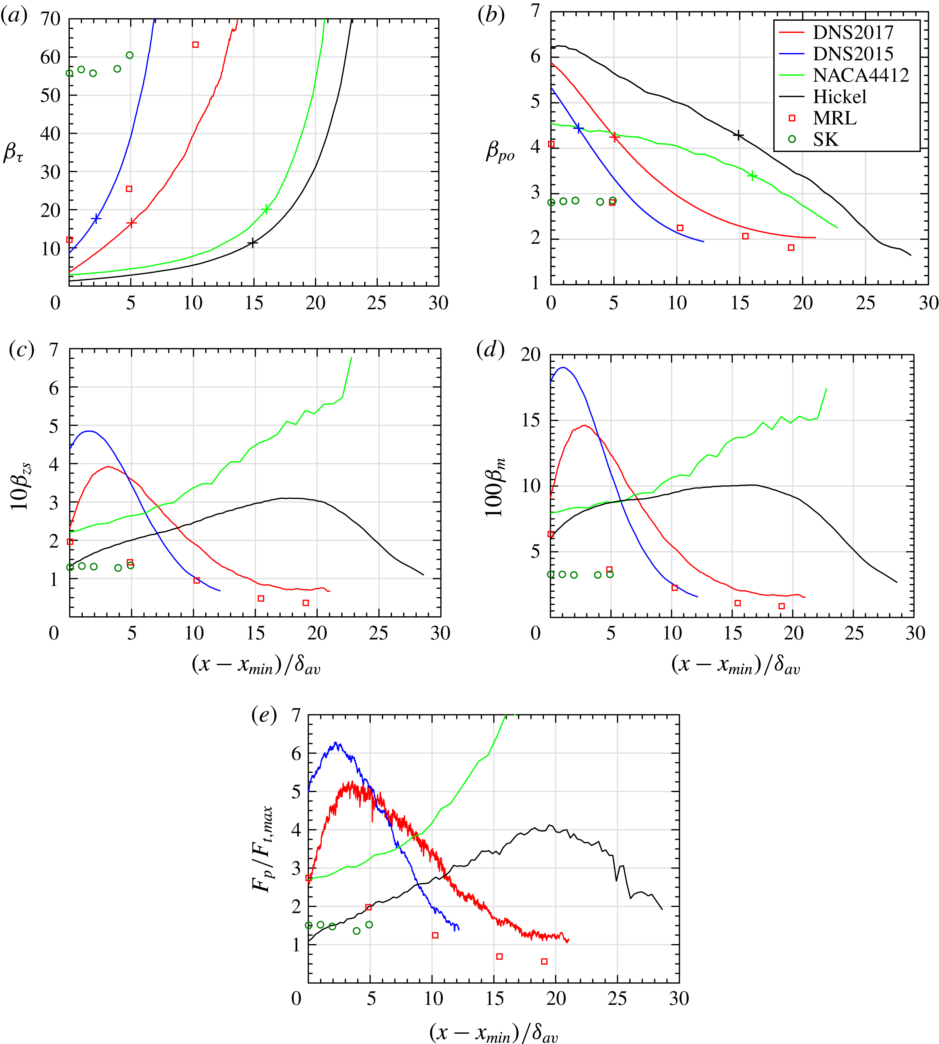
Figure 10(a–d) shows the streamwise evolution of the pressure-gradient parameters $\unicode[STIX]{x1D6FD}_{\unicode[STIX]{x1D70F}}$ , $\unicode[STIX]{x1D6FD}_{po}$ , $\unicode[STIX]{x1D6FD}_{zs}$ and $\unicode[STIX]{x1D6FD}_{m}$ for the different flows. It was demonstrated in the previous section that these pressure-gradient parameters should represent the ratio of the order of magnitude of the pressure force to the order of magnitude of the apparent turbulent force in the outer region:

(5.1) $$\begin{eqnarray}O\left(\frac{\text{d}p_{e}}{\text{d}x}\right)\bigg/O\left(\unicode[STIX]{x1D70C}\frac{\unicode[STIX]{x2202}\langle uv\rangle }{\unicode[STIX]{x2202}y}\right).\end{eqnarray}$$

Figure 10(e) shows directly this ratio in the form of the pressure force over the maximum of the Reynolds shear stress gradient in the outer region – note that the momentum balance of flow DNS2015 was studied in detail by Gungor et al. (Reference Gungor, Maciel, Simens and Soria2016). If we focus first on figure 10(e), we see that the ratio of forces remains fairly constant for flow SK, a result that is expected since dynamic equilibrium is by essence the definition of an equilibrium TBL. The non-equilibrium nature of the five other APG TBLs is reflected by the important streamwise variation of the ratio of forces. For four of the present non-equilibrium TBLs – DNS2017, DNS2015, Hickel and MRL – the importance of the pressure force with respect to the turbulent force decreases in the outer region as the velocity defect increases in the large-defect zones of these flows (downstream). Flow NACA4412 behaves differently in that the dominance of the pressure force keeps increasing all the way to the airfoil trailing edge.

Figure 10.

Outer region pressure-gradient parameter $\unicode[STIX]{x1D6FD}_{o}$ with $U_{o}$ taken as (a) $u_{\unicode[STIX]{x1D70F}}$ , (b) $U_{po}$ , (c) $U_{zs}$ and (d) $U_{m}$ . Note that $\unicode[STIX]{x1D6FD}_{o}=0$ for ZPG TBLs. The $+$ signs on the lines mark the positions where $H=1.6$ . (e) Ratio of the pressure force $F_{p}$ to the maximum Reynolds shear stress gradient in the outer region $F_{t,max}$ .

In figure 10(a,b), $\unicode[STIX]{x1D6FD}_{\unicode[STIX]{x1D70F}}$ and $\unicode[STIX]{x1D6FD}_{po}$ are shown for the whole selected streamwise region of each flow – the same one used in the previous figures – even if these pressure-gradient parameters are not valid over the whole region of the APG boundary layers. For instance, figure 10(e) indicates that $\unicode[STIX]{x1D6FD}_{\unicode[STIX]{x1D70F}}$ no longer represents the order of magnitude of the ratio of pressure to turbulent forces in the outer region when $H$ exceeds approximately 1.6, and this is true for all APG TBLs studied here, including the quasi-equilibrium TBL of SK (the point where $H=1.6$ is illustrated with + signs in figure 10(a,b), for the flows obtained numerically). The fact that $\unicode[STIX]{x1D6FD}_{\unicode[STIX]{x1D70F}}$ loses its meaning as the ratio of pressure to turbulent forces for $H>1.6$ is consistent with the fact that $u_{\unicode[STIX]{x1D70F}}$ is no longer a scale of the mean velocity defect and Reynolds stresses for roughly $H>1.8$ , as shown in § 3. In the case of MRL flow, $\unicode[STIX]{x1D6FD}_{\unicode[STIX]{x1D70F}}$ has the meaning of the ratio of the orders of magnitude of pressure and turbulent forces only for the first data point. Note that $\unicode[STIX]{x1D6FD}_{RC}$ , shown in figure 1(c), behaves similarly to $\unicode[STIX]{x1D6FD}_{\unicode[STIX]{x1D70F}}$ . The meaning of $\unicode[STIX]{x1D6FD}_{RC}$ and $\unicode[STIX]{x1D6FD}_{\unicode[STIX]{x1D70F}}$ is discussed further below.

One cannot normally use $\unicode[STIX]{x1D6FD}_{po}$ for small-defect TBLs since $U_{po}$ is not a valid outer velocity scale for very small pressure gradients. A comparison of figure 10(b) and figure 10(e) shows that, in the small-defect zones of these flows (upstream segments of the non-equilibrium TBLs), $\unicode[STIX]{x1D6FD}_{po}$ retains the correct order of magnitude of the ratio of pressure to turbulent forces, but the streamwise evolutions and magnitude ranking between flows are wrong. Nonetheless, $\unicode[STIX]{x1D6FD}_{\unicode[STIX]{x1D70F}}$ (when it is valid) and $\unicode[STIX]{x1D6FD}_{po}$ are the ones that give the right order of magnitude of the ratio of forces. In order to reflect the correct order of magnitude, $\unicode[STIX]{x1D6FD}_{zs}$ and $\unicode[STIX]{x1D6FD}_{m}$ have to be multiplied by 10 and 100, respectively, as is done in figure 10(c,d) – we use powers of 10 since this is an order-of-magnitude analysis. This stems from the fact that the scaled Reynolds shear stress gradient – $\unicode[STIX]{x2202}R_{12}^{\ast }/\unicode[STIX]{x2202}\unicode[STIX]{x1D702}$ in equation (4.11) – is of order of magnitude one in the outer region if $U_{o}$ equals $u_{\unicode[STIX]{x1D70F}}$ or $U_{po}$ in the domains of validity of these velocity scales (roughly $H<1.8$ and $H>1.8$ , respectively) and of order of magnitude 0.1 and 0.01 for all types of TBLs if $U_{o}$ equals $U_{zs}$ or $U_{m}$ . These orders of magnitude can be appreciated from figure 11 in the case of $U_{po}$ and $U_{zs}$ , and indirectly from the Reynolds shear stress profiles of figure 5 for flow DNS2017.

In § 3, we emphasized and showed that the outer velocity scales only reveal the order of magnitude of the mean velocity defect and the Reynolds stresses – they do not reveal scale invariance or universal similarity. Consequently, it was expected that the pressure-gradient parameter would only reflect the order of magnitude of the ratio of pressure to turbulent forces in the outer region, not a precise value of this ratio. However, quite to our astonishment, a comparison of figure 10(c) with figure 10(e) clearly indicates that $\unicode[STIX]{x1D6FD}_{zs}$ represents very well this ratio. Thus $\unicode[STIX]{x1D6FD}_{zs}$ permits one to follow the streamwise evolution of the ratio of pressure to turbulent forces, and to compare it between flows. Such a good correspondence is impressive and unexpected. As we will see below, the same is also true for $\unicode[STIX]{x1D6FC}_{zs}$ and $Re_{zs}$ . These three parameters can therefore be used to follow the streamwise evolution of the streamwise mean momentum balance – in a global sense – in the outer region.

The second best representation of the ratio of pressure to turbulent forces is given by $\unicode[STIX]{x1D6FD}_{m}$ , which is less accurate than $\unicode[STIX]{x1D6FD}_{zs}$ in representing the upstream evolution and magnitude of the ratio of forces for flow Hickel, and the downstream part of flow NACA4412. In figure 10(b), if we focus on the zones where $\unicode[STIX]{x1D6FD}_{po}$ should be valid (right of the $+$ signs for the numerical flows, last four data points for MRL, and all data points for SK), we see that $\unicode[STIX]{x1D6FD}_{po}$ is much less accurate than $\unicode[STIX]{x1D6FD}_{zs}$ and $\unicode[STIX]{x1D6FD}_{m}$ in representing the streamwise evolutions and magnitudes of the ratio of forces. In fact, $\unicode[STIX]{x1D6FD}_{po}$ gives the wrong streamwise evolution and magnitude for flow NACA4412.

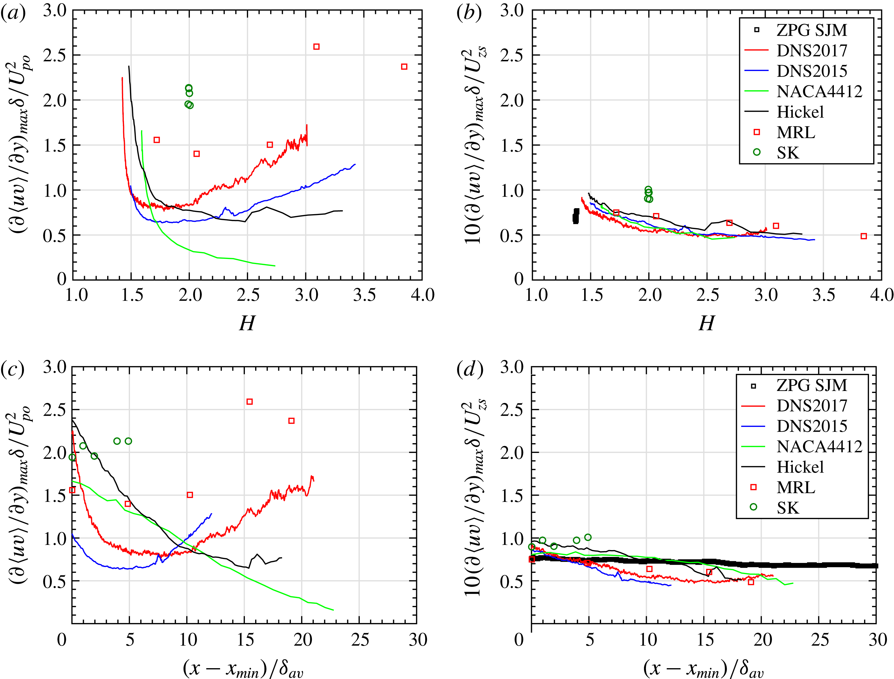
The explanation for these results lies in the fact that $U_{zs}^{2}$ scales extremely well the amplitude of the Reynolds shear stress gradient in the outer region. This can be appreciated with figure 11, where a comparison is made between the maximum value of the Reynolds shear stress gradient normalized with $U_{po}^{2}$ and $U_{zs}^{2}$ . For all flows and all velocity-defect conditions, this maximum value follows almost a single curve when scaled with $U_{zs}^{2}$ and expressed as a function of $H$ (figure 11 b). Moreover, it is almost constant, only varying between 0.5 and 1.0 (with $U_{zs}^{2}$ divided by 10). Consequently, with $U_{o}=U_{zs}$ , the non-dimensional Reynolds shear stress gradient in (4.11) has an almost constant maximum amplitude in the outer region. Therefore $\unicode[STIX]{x1D6FD}_{zs}$ gives an almost exact representation of the ratio of pressure force to maximum turbulent force.

Figure 11.

Maximum value of the Reynolds shear stress gradient in the outer region normalized with (a) $U_{po}^{2}$ and (b) $U_{zs}^{2}$ as a function of $H$ . Same ordinates for (c,d) but as a function of $(x_{min}-x)/\unicode[STIX]{x1D6FF}_{av}.$

Figures 11(c) and 11(d) are equivalent to figures 11(a) and 11(b) respectively, but with the streamwise position as abscissa instead of $H$ . They are only shown to allow a direct comparison with figures 10 and 12. Figures 11(a) and 11(b) are more useful, since they reveal the scaling trend as a function of the mean velocity defect.

The pressure-gradient parameters that involve the wall shear stress, the Rotta–Clauser pressure-gradient parameter $\unicode[STIX]{x1D6FD}_{RC}$ and $\unicode[STIX]{x1D6FD}_{\unicode[STIX]{x1D70F}}$ , change meaning when the mean velocity defect is important. As we have seen in § 3, with figure 6 as an example, $\unicode[STIX]{x1D6FD}_{RC}$ can reflect – but in some cases only, as explained below – the state of a TBL from small defect to large defect. In other words, $\unicode[STIX]{x1D6FD}_{RC}$ and $\unicode[STIX]{x1D6FD}_{\unicode[STIX]{x1D70F}}$ are indicators of the cumulative impact (local and upstream history) of the pressure gradient on the boundary layer. However, they are imperfect indicators of such an impact because they comprise a parameter that is independent of history effects: the local value of the pressure gradient. In the case of the present non-equilibrium TBLs, $\unicode[STIX]{x1D6FD}_{RC}$ and $\unicode[STIX]{x1D6FD}_{\unicode[STIX]{x1D70F}}$ reflect well the cumulative impact of the pressure gradient but this is only because these are flows with a monotonic increase of $\unicode[STIX]{x1D6FD}_{RC}$ (monotonic increase of $H$ ). An example of a situation where $\unicode[STIX]{x1D6FD}_{RC}$ and $\unicode[STIX]{x1D6FD}_{\unicode[STIX]{x1D70F}}$ fail to reflect the cumulative impact of the pressure gradient is a TBL that is still responding to an upstream pressure gradient although the pressure gradient has returned to zero, hence $\unicode[STIX]{x1D6FD}_{RC}=\unicode[STIX]{x1D6FD}_{\unicode[STIX]{x1D70F}}=0$ . This example shows that the shape factor $H$ is a better indicator of the cumulative impact (local and upstream history) of the pressure gradient on the boundary layer. Moreover, its definition does not assume any choice of scales, contrary to $\unicode[STIX]{x1D6FD}_{RC}$ and the Rotta–Clauser defect shape factor $G$ .

The issue of the physical meaning of $\unicode[STIX]{x1D6FD}_{RC}$ is important since it is probably the most widely used pressure-gradient parameter. To the authors’ knowledge, the only other situation where $\unicode[STIX]{x1D6FD}_{RC}$ has a clear meaning is in the context of equilibrium TBLs. In this context, Mellor & Gibson (Reference Mellor and Gibson1966), Schlichting & Gersten (Reference Schlichting and Gersten2000) and Maciel et al. (Reference Maciel, Rossignol and Lemay2006b ) rewrite the ordinary differential equation of motion of equilibrium TBLs in order to bring out $\unicode[STIX]{x1D6FD}_{RC}$ as one of the similarity parameters. However, it is important to insist that, even in this case, $\unicode[STIX]{x1D6FD}_{RC}$ does not come out naturally as one of the similarity parameters; much in the same manner as in the present analysis $\unicode[STIX]{x1D6FD}_{o}$ clearly does not have to be  $\unicode[STIX]{x1D6FD}_{RC}$ .

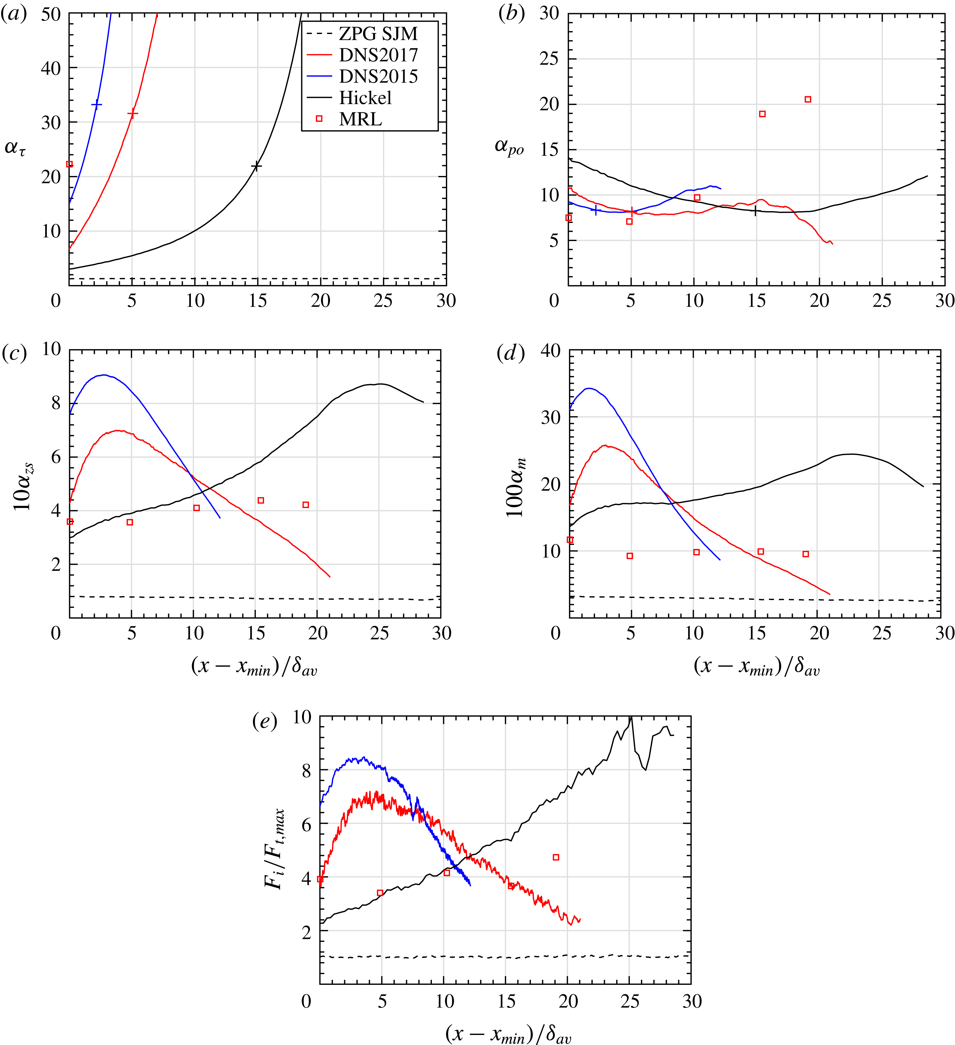
The inertial parameter is now discussed. Figure 12(a–d) shows the streamwise evolution of the inertial parameters $\unicode[STIX]{x1D6FC}_{\unicode[STIX]{x1D70F}}$ , $\unicode[STIX]{x1D6FC}_{po}$ , $\unicode[STIX]{x1D6FC}_{zs}$ and $\unicode[STIX]{x1D6FC}_{m}$ for the flows for which $V$ was available. These parameters should represent the ratio of the order of magnitude of the inertial force (streamwise mean momentum advection) to the order of magnitude of the apparent turbulent force in the outer region:

(5.2) $$\begin{eqnarray}O\left(U\frac{\unicode[STIX]{x2202}U}{\unicode[STIX]{x2202}x}+V\frac{\unicode[STIX]{x2202}U}{\unicode[STIX]{x2202}y}\right)\bigg/O\left(\frac{\unicode[STIX]{x2202}\langle uv\rangle }{\unicode[STIX]{x2202}y}\right).\end{eqnarray}$$

Figure 12(e) shows directly this ratio in the form of the maximum mean momentum advection over the maximum Reynolds shear stress gradient in the outer region. Note that, in order to reduce considerably the uncertainty in the computation of these maxima, the profiles of $U$ , $V$ and $\langle uv\rangle$ were smoothed with cubic splines before computing the derivatives.

Figure 12.

Outer region parameter $\unicode[STIX]{x1D6FC}_{o}$ with $U_{o}$ taken as (a) $u_{\unicode[STIX]{x1D70F}}$ , (b)  $U_{po}$ , (c) $U_{zs}$ and (d) $U_{m}$ . The $+$ signs on the lines mark the positions where $H=1.6$ . (e) Ratio of the maximum inertial force $F_{i,max}$ to the maximum Reynolds shear stress gradient $F_{t,max}$ in the outer region.

Similarly to what was obtained for the pressure-gradient parameter, we see that $\unicode[STIX]{x1D6FC}_{zs}$ represents very well the streamwise evolution of the ratio of the inertial force to the apparent turbulent force in the outer region. Again, this is quite an impressive result. The other inertial parameters, $\unicode[STIX]{x1D6FC}_{\unicode[STIX]{x1D70F}}$ , $\unicode[STIX]{x1D6FC}_{po}$ and $\unicode[STIX]{x1D6FC}_{m}$ , represent the order of magnitude of the ratio of forces (when they are valid) but nothing more. As for the pressure-gradient parameters, $\unicode[STIX]{x1D6FC}_{\unicode[STIX]{x1D70F}}$ no longer reflects this order of magnitude when roughly $H>1.6$ . This is the case for all data points of flow SK and the last four data points of MRL.

We see from figure 12(e) (or figure 12 c) that inertia tends to dominate the apparent turbulent force in the APG TBLs, in contrast to the situation in the ZPG TBL, where the two forces have about the same magnitude. Like the ratio of pressure to turbulent forces, the streamwise evolution of the ratio of inertia to turbulent forces varies considerably from one APG TBL to another.

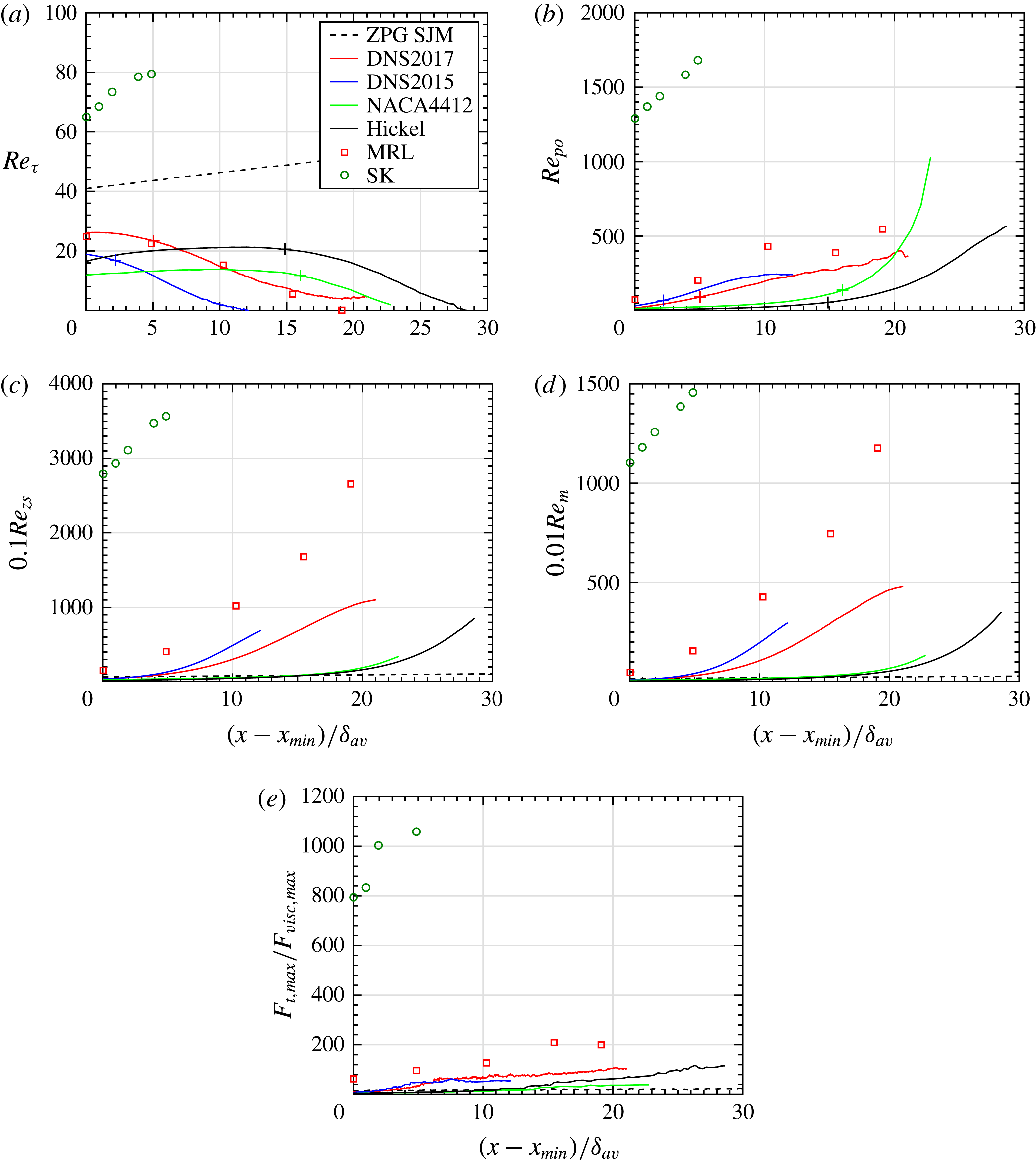
Figure 13 presents the streamwise evolution of the Reynolds numbers $Re_{\unicode[STIX]{x1D70F}}$ , $Re_{po}$ , $Re_{zs}$ and $Re_{m}$ for the different flows. Recall that these Reynolds numbers should represent the ratio of the order of magnitude of the Reynolds shear stress gradient (apparent turbulent force) to the order of magnitude of the viscous force in the outer region:

(5.3) $$\begin{eqnarray}O\left(\unicode[STIX]{x1D70C}\frac{\unicode[STIX]{x2202}\langle uv\rangle }{\unicode[STIX]{x2202}y}\right)\bigg/O\left(\unicode[STIX]{x1D707}\frac{\unicode[STIX]{x2202}^{2}U}{\unicode[STIX]{x2202}y^{2}}\right).\end{eqnarray}$$

Figure 13(e) presents this ratio in the form of the maximum Reynolds shear stress gradient over the maximum viscous shear stress gradient in the outer region. Again, in order to reduce considerably the uncertainty in the computation of these maxima, the profiles of $U$ and $\langle uv\rangle$ were smoothed with cubic splines before computing the derivatives. Even so, the uncertainty in the value of $\unicode[STIX]{x2202}^{2}U/\unicode[STIX]{x2202}y^{2}$ is high, in particular for the two experimental databases. Consequently, the results presented in figure 13(e) have to be analysed with caution due to their high uncertainty. That being said, these results indicate that, as expected, the SK flow has the highest turbulent Reynolds number in the outer region by far, followed by MRL. DNS2017 and Hickel flows appear to be globally at a slightly higher outer Reynolds number than DNS2015, NACA4412 and ZPG SJM.

Figure 13.

Outer region Reynolds number $Re_{o}$ with $U_{o}$ taken as (a)  $u_{\unicode[STIX]{x1D70F}}$ , (b) $U_{po}$ , (c) $U_{zs}$ and (d) $U_{m}$ . Note that $Re_{po}=0$ for ZPG TBLs. The $+$ signs on the lines mark the positions where $H=1.6$ . (e) Ratio of the maximum Reynolds shear stress gradient $F_{t,max}$ to the maximum viscous shear stress gradient $F_{visc,max}$ in the outer region.

Despite the aforementioned uncertainty, we can probably conclude that the order of magnitude of the ratio of the maximum Reynolds shear stress gradient to the maximum viscous force in the outer region is well represented by $Re_{po}$ , $Re_{zs}$ and $Re_{m}$ . However, $Re_{po}$ overestimates this ratio of forces in the downstream part of flow NACA4412. Note that the streamwise evolution of $\unicode[STIX]{x1D6FD}_{po}$ was also wrong for NACA4412. It is therefore possible that we have incorrect $\text{d}p_{e}/\text{d}x$ values for this flow even though these values have been checked. As for $Re_{zs}$ and $Re_{m}$ , they seem to overestimate the force ratio in all non-equilibrium TBLs when the velocity defect becomes important. However, they allow the force ratio of the ZPG TBL to be compared with that of the other flows, something that $Re_{po}$ cannot do.

As with the other two non-dimensional parameters, $Re_{\unicode[STIX]{x1D70F}}$ loses its meaning as the ratio of turbulent to viscous forces for $H>1.6$ . This is the case for all data points of flow SK and the last four data points of MRL. For all non-equilibrium TBLs, the loss of significance of $Re_{\unicode[STIX]{x1D70F}}$ is reflected by the fact that $Re_{\unicode[STIX]{x1D70F}}$ starts decreasing as the mean velocity defect increases, while $Re_{po}$ , $Re_{zs}$ and $Re_{m}$ clearly indicate that the outer region Reynolds number $Re_{o}$ keeps increasing.

The most commonly used local boundary layer Reynolds number is $Re_{\unicode[STIX]{x1D703}}$ , shown in figure 1(a), and already discussed in § 2. Performing an analysis similar to that done in § 4, we can show that $Re_{\unicode[STIX]{x1D703}}$ is also the ratio of apparent turbulent forces to viscous forces in the outer region, if we use $\unicode[STIX]{x1D703}$ as the reference wall-normal length $L_{o}$ and $U_{e}$ as the reference velocity for the Reynolds shear stress. However, as discussed previously, $\unicode[STIX]{x1D703}$ is not a proper outer length scale and $U_{e}$ is not an outer velocity scale of the Reynolds shear stress. For these reasons, a comparison of $Re_{\unicode[STIX]{x1D703}}$ (figure 1 a) with the force ratio (figure 13 e) shows that $Re_{\unicode[STIX]{x1D703}}$ does not give the correct order of magnitude of this ratio. Moreover, it overestimates the force ratio of the small-defect flows/zones (such as the ZPG TBL) in comparison to the large-defect flows/zones. The streamwise evolutions are however well represented in the large-defect flows/zones.