1 Introduction
Electromagnetic forcing of conducting fluids can be used to induce their motion in conditions where driving them mechanically is either impossible due to an aggressive environment or extreme confinement, or undesirable because of the intrusive nature of mechanical excitation. Various metallurgical processes occurring at high temperatures (Moffatt Reference Moffatt1991) or mixing of conducting fluids in microfluidic devices (Pérez-Barrera, Ortiz & Cuevas Reference Pérez-Barrera, Ortiz, Cuevas, Klapp, Sigalotti, Ovando, Villa and Chavarría2016) offer examples of the former while the latter is frequently the case in physical modelling of atmospheric phenomena in laboratory conditions, which has been pioneered by Soviet researchers (Dovzhenko, Novikov & Obukhov Reference Dovzhenko, Novikov and Obukhov1979; Dovzhenko, Obukhov & Ponomarev Reference Dovzhenko, Obukhov and Ponomarev1981; Dovzhenko, Krymov & Ponomarev Reference Dovzhenko, Krymov and Ponomarev1984; Krymov Reference Krymov1989; Manin Reference Manin1989; Dolzhanskii, Krymov & Manin Reference Dolzhanskii, Krymov and Manin1990), see also Bondarenko, Gak & Gak (Reference Bondarenko, Gak and Gak2002), Kenjeres (Reference Kenjeres2011), and which has inspired the current study. A more detailed review of relevant applications can be found in our previous publication Suslov, Pérez-Barrera & Cuevas (Reference Suslov, Pérez-Barrera and Cuevas2017).
Conducting fluids that can be driven electromagnetically generally fall into two wide classes characterised the value of their electric conductivity. The first group includes good conductors, such as liquid metals and melts, while common representatives of the second class, which are the subject of this study, are electrolytes (diluted water solutions of salts) that have a much smaller conductivity. Under standard conditions at laboratory or industrial scales, flows of both types of fluid are characterised by low values of the magnetic Reynolds number, which indicates that magnetic field induced by the motion of an electrically conducting fluid is much smaller than the applied field. This fact simplifies the analysis by justifying the use of the so-called magneto-static approximation (Davidson Reference Davidson2001). When an electrolyte carrying an electric current is placed in an external magnetic field created by a permanent magnet or electromagnet, a driving electromagnetic Lorentz force arises. Since the conductivity of electrolytes is relatively small (compared to those of liquid metals), the induced currents remain small and have a negligible effect on fluid flows.
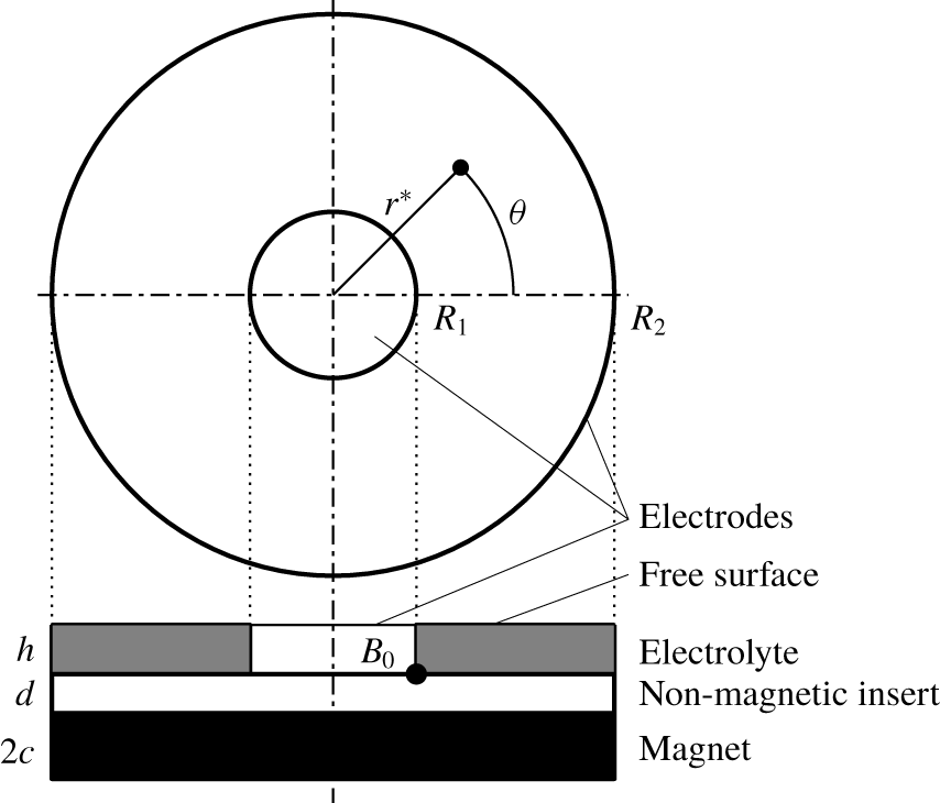
Experimentally, a flow of an electrolyte is easy to create in an annular layer over an insulating bottom contained between two co-axial cylindrical electrodes (Digilov Reference Digilov2007; Pérez-Barrera et al. Reference Pérez-Barrera, Pérez-Espinoza, Ortiz, Ramos and Cuevas2015, Reference Pérez-Barrera, Ortiz, Cuevas, Klapp, Sigalotti, Ovando, Villa and Chavarría2016). If it is placed on top of a vertically polarised magnet, the interaction of the radial electric current between electrodes and magnetic field gives rise to an azimuthal Lorentz body force that drives the flow. A schematic view of such an experimental set-up, described in detail in our previous work (Suslov et al. Reference Suslov, Pérez-Barrera and Cuevas2017), is shown in figure 1. When the radial current is switched on, an azimuthal flow is established. The investigation undertaken in Suslov et al. (Reference Suslov, Pérez-Barrera and Cuevas2017) revealed the existence of two solutions, designated there as Type 1 and Type 2 (we keep this terminology here). The topological difference between them will be reviewed in § 5. Despite the simple geometry and large body of literature existing on rotating flows, the analysis undertaken in Suslov et al. (Reference Suslov, Pérez-Barrera and Cuevas2017) led us to conclude that neither of these two solutions have a direct analogy with any of the well-known flow situations such as Ekman (Ekman Reference Ekman1905; Lilly Reference Lilly1966; Greenspan Reference Greenspan1968; Faller Reference Faller1991), Bödewadt (Bödewadt Reference Bödewadt1940; MacKerrell Reference MacKerrell2005) or Stewartson (Stewartson Reference Stewartson1957; Schaeffer & Cardin Reference Schaeffer and Cardin2005) boundary layers or flows between rotating disks (Moisy et al. Reference Moisy, Doaré, Pasutto, Daube and Rabaud2004). A comprehensive stability study of annular flows driven by a body rather than surface forces (e.g. the instability of a Taylor–Couette flow) has also received relatively little attention and, to the best of our knowledge, is limited to flows between infinitely long coaxial cylinders or finite cylinders with solid caps (Qin & Bau Reference Qin and Bau2012, e.g.). A shallow fluid depth and the presence of a free surface are the main features distinguishing the current set-up from those considered in the stability context previously. A recent attempt at a stability investigation of a flow in such a geometry undertaken by Antar, Lalti & Habchi (Reference Antar, Lalti and Habchi2019), of which we became aware after the work on this paper had been completed, has resulted in erroneous conclusions about the physical nature of the observed flows and instability, which will become clear from the analysis we present here.
Experiments show that, when the strength of the current across the shallow annular electrolyte layer (and thus the speed of azimuthal flow) increases, a robust system of vortices rotating in the opposite direction to the global azimuthal flow arises near the outer cylindrical wall. The main conclusion made in Suslov et al. (Reference Suslov, Pérez-Barrera and Cuevas2017) was that the appearance of such vortices cannot be explained using a thin layer approximation or assuming that the base flow on the background of which the vortices develop is unidirectional. This motivated us to undertake a fully three-dimensional study of the stability of the axisymmetric toroidal basic flow reviewed in § 3. This analysis is reported in §§ 4 and 5. In § 6 we start with linear stability equations of § 4 to derive perturbation energy balance equations. These enable us to unambiguously identify the physical mechanism responsible for the formation of the experimentally observed vortices. Linear stability results of § 5 led us to hypothesise that the Type 1 and Type 2 axisymmetric basic flow solutions reported in Suslov et al. (Reference Suslov, Pérez-Barrera and Cuevas2017) appear as a result of a saddle-node bifurcation. To the best of our knowledge such a bifurcation has not been reported for other rotational flows in similar geometries. Thus, in § 7, we use a weakly nonlinear analysis to derive a canonical amplitude-type equation to confirm its presence. We subsequently use this analysis in § 8 to provide a further qualitative insight into the abrupt transition between the Type 1 and Type 2 solutions that occurs at smaller values of the current driving the basic flow. The major conclusions are given in § 9.
2 Problem formulation and governing equations
Sketch of the problem geometry. The azimuthal motion of electrolyte contained in a layer of thickness  $h$ between vertical cylindrical electrodes located at
 $r^{\ast }=R_{1}$ and
 $r^{\ast }=R_{2}$ is caused by a Lorentz body force arising due to the interaction of the radial electric current flowing between the electrodes and the predominantly vertical magnetic field characterised by the amplitude
 $B_{0}$ evaluated at the indicated corner point. The magnetic field is created by a disk magnet of radius
 $R_{2}$ and height
 $2c$ placed at a distance
 $d$ under the bottom of the electrolyte layer.

Consider an annular free-surface layer of electrolyte above a non-conducting stationary solid bottom. Laterally, the layer is bounded by two vertical co-axial cylindrical electrodes, as shown in figure 1. The electrolyte has density  $\unicode[STIX]{x1D70C}$, electric conductivity
 $\unicode[STIX]{x1D70E}_{e}$ and dynamic viscosity
 $\unicode[STIX]{x1D707}$. The system is placed above a vertically polarised permanent disk magnet that creates a predominantly vertical non-uniform magnetic field. The spatial distribution of the field used to obtain all numerical results here is computed using the same procedure and for the same geometrical dimensions of an experimental set-up described in Suslov et al. (Reference Suslov, Pérez-Barrera and Cuevas2017), see table 1 therein.
As discussed in Suslov et al. (Reference Suslov, Pérez-Barrera and Cuevas2017), when an electric potential difference  $\unicode[STIX]{x0394}\unicode[STIX]{x1D719}_{0}$ is applied between the electrodes, the total current
 $$\begin{eqnarray}I_{0}\approx \frac{2\unicode[STIX]{x03C0}\unicode[STIX]{x1D70E}_{e}h\unicode[STIX]{x0394}\unicode[STIX]{x1D719}_{0}}{\ln (R_{2}/R_{1})},\end{eqnarray}$$
flows mostly radially through the layer between them. The interaction of the current and the applied magnetic field creates a Lorentz force  $\boldsymbol{F}_{L}=\boldsymbol{j}\times \boldsymbol{B}$, where
 $\boldsymbol{j}$ and
 $\boldsymbol{B}$ are the applied current density and the magnetic induction field, respectively. This predominantly unidirectional azimuthal force drives the flow, the stability of which we investigate here.
Under the small magnetic Reynolds number approximation (Davidson Reference Davidson2001; Pérez-Barrera et al. Reference Pérez-Barrera, Ortiz, Cuevas, Klapp, Sigalotti, Ovando, Villa and Chavarría2016) the fluid motion is governed by the non-dimensional Poisson’s equation for the electric potential, the momentum equations and the continuity equation for an incompressible fluid. They are written in cylindrical coordinates as
 $$\begin{eqnarray}\displaystyle & & \displaystyle \displaystyle \frac{\unicode[STIX]{x2202}^{2}\unicode[STIX]{x1D719}}{\unicode[STIX]{x2202}z^{2}}+\unicode[STIX]{x1D716}^{2}\left(\frac{\unicode[STIX]{x2202}^{2}\unicode[STIX]{x1D719}}{\unicode[STIX]{x2202}r^{2}}+\frac{1}{r}\frac{\unicode[STIX]{x2202}\unicode[STIX]{x1D719}}{\unicode[STIX]{x2202}r}+\frac{1}{r^{2}}\frac{\unicode[STIX]{x2202}^{2}\unicode[STIX]{x1D719}}{\unicode[STIX]{x2202}\unicode[STIX]{x1D703}^{2}}\right)=\unicode[STIX]{x1D716}^{2}Ha^{2}\left[B_{r}\left(\frac{\unicode[STIX]{x1D716}^{2}}{r}\frac{\unicode[STIX]{x2202}u_{z}}{\unicode[STIX]{x2202}\unicode[STIX]{x1D703}}-\frac{\unicode[STIX]{x2202}u_{\unicode[STIX]{x1D703}}}{\unicode[STIX]{x2202}z}\right)\right.\nonumber\\ \displaystyle & & \displaystyle \quad \quad \left.+\,B_{z}\displaystyle \left(\frac{\unicode[STIX]{x2202}u_{\unicode[STIX]{x1D703}}}{\unicode[STIX]{x2202}r}+\frac{u_{\unicode[STIX]{x1D703}}}{r}-\frac{1}{r}\frac{\unicode[STIX]{x2202}u_{r}}{\unicode[STIX]{x2202}\unicode[STIX]{x1D703}}\right)\right],\end{eqnarray}$$
 $$\begin{eqnarray}\displaystyle & & \displaystyle \displaystyle \frac{\unicode[STIX]{x2202}u_{r}}{\unicode[STIX]{x2202}t}+u_{r}\frac{\unicode[STIX]{x2202}u_{r}}{\unicode[STIX]{x2202}r}+\frac{u_{\unicode[STIX]{x1D703}}}{r}\frac{\unicode[STIX]{x2202}u_{r}}{\unicode[STIX]{x2202}\unicode[STIX]{x1D703}}-\frac{u_{\unicode[STIX]{x1D703}}^{2}}{r}+u_{z}\frac{\unicode[STIX]{x2202}u_{r}}{\unicode[STIX]{x2202}z}=-\frac{1}{Fr^{2}}\frac{\unicode[STIX]{x2202}p}{\unicode[STIX]{x2202}r}+\frac{1}{\unicode[STIX]{x1D716}^{2}Re}j_{\unicode[STIX]{x1D703}}B_{z}\nonumber\\ \displaystyle & & \displaystyle \qquad +\,\frac{1}{Re}\left(\frac{\unicode[STIX]{x2202}^{2}u_{r}}{\unicode[STIX]{x2202}r^{2}}+\frac{1}{r}\frac{\unicode[STIX]{x2202}u_{r}}{\unicode[STIX]{x2202}r}-\frac{u_{r}}{r^{2}}+\frac{1}{r^{2}}\frac{\unicode[STIX]{x2202}^{2}u_{r}}{\unicode[STIX]{x2202}\unicode[STIX]{x1D703}^{2}}-\frac{2}{r^{2}}\frac{\unicode[STIX]{x2202}u_{\unicode[STIX]{x1D703}}}{\unicode[STIX]{x2202}\unicode[STIX]{x1D703}}+\frac{1}{\unicode[STIX]{x1D716}^{2}}\frac{\unicode[STIX]{x2202}^{2}u_{r}}{\unicode[STIX]{x2202}z^{2}}\right),\end{eqnarray}$$
 $$\begin{eqnarray}\displaystyle & & \displaystyle \displaystyle \frac{\unicode[STIX]{x2202}u_{\unicode[STIX]{x1D703}}}{\unicode[STIX]{x2202}t}+u_{r}\frac{\unicode[STIX]{x2202}u_{\unicode[STIX]{x1D703}}}{\unicode[STIX]{x2202}r}+\frac{u_{\unicode[STIX]{x1D703}}}{r}\frac{\unicode[STIX]{x2202}u_{\unicode[STIX]{x1D703}}}{\unicode[STIX]{x2202}\unicode[STIX]{x1D703}}+\frac{u_{r}u_{\unicode[STIX]{x1D703}}}{r}+u_{z}\frac{\unicode[STIX]{x2202}u_{\unicode[STIX]{x1D703}}}{\unicode[STIX]{x2202}z}=-\frac{1}{Fr^{2}}\frac{1}{r}\frac{\unicode[STIX]{x2202}p}{\unicode[STIX]{x2202}\unicode[STIX]{x1D703}}+\frac{1}{\unicode[STIX]{x1D716}^{2}Re}(j_{z}B_{r}-j_{r}B_{z})\nonumber\\ \displaystyle & & \displaystyle \qquad +\,\frac{1}{Re}\left(\frac{\unicode[STIX]{x2202}^{2}u_{\unicode[STIX]{x1D703}}}{\unicode[STIX]{x2202}r^{2}}+\frac{1}{r}\frac{\unicode[STIX]{x2202}u_{\unicode[STIX]{x1D703}}}{\unicode[STIX]{x2202}r}-\frac{u_{\unicode[STIX]{x1D703}}}{r^{2}}+\frac{1}{r^{2}}\frac{\unicode[STIX]{x2202}^{2}u_{\unicode[STIX]{x1D703}}}{\unicode[STIX]{x2202}\unicode[STIX]{x1D703}^{2}}+\frac{2}{r^{2}}\frac{\unicode[STIX]{x2202}u_{r}}{\unicode[STIX]{x2202}\unicode[STIX]{x1D703}}+\frac{1}{\unicode[STIX]{x1D716}^{2}}\frac{\unicode[STIX]{x2202}^{2}u_{\unicode[STIX]{x1D703}}}{\unicode[STIX]{x2202}z^{2}}\right),\end{eqnarray}$$
 $$\begin{eqnarray}\displaystyle & & \displaystyle \frac{\unicode[STIX]{x2202}u_{z}}{\unicode[STIX]{x2202}t}+u_{r}\frac{\unicode[STIX]{x2202}u_{z}}{\unicode[STIX]{x2202}r}+\frac{u_{\unicode[STIX]{x1D703}}}{r}\frac{\unicode[STIX]{x2202}u_{z}}{\unicode[STIX]{x2202}\unicode[STIX]{x1D703}}+u_{z}\frac{\unicode[STIX]{x2202}u_{z}}{\unicode[STIX]{x2202}z}=-\frac{1}{Fr^{2}\unicode[STIX]{x1D716}^{2}}\frac{\unicode[STIX]{x2202}p}{\unicode[STIX]{x2202}z}-\frac{1}{\unicode[STIX]{x1D716}^{2}Re}j_{\unicode[STIX]{x1D703}}B_{r}\nonumber\\ \displaystyle & & \displaystyle \qquad +\,\frac{1}{Re}\left(\frac{\unicode[STIX]{x2202}^{2}u_{z}}{\unicode[STIX]{x2202}r^{2}}+\frac{1}{r}\frac{\unicode[STIX]{x2202}u_{z}}{\unicode[STIX]{x2202}r}+\frac{1}{r^{2}}\frac{\unicode[STIX]{x2202}^{2}u_{z}}{\unicode[STIX]{x2202}\unicode[STIX]{x1D703}^{2}}+\frac{1}{\unicode[STIX]{x1D716}^{2}}\frac{\unicode[STIX]{x2202}^{2}u_{z}}{\unicode[STIX]{x2202}z^{2}}\right),\end{eqnarray}$$
 $$\begin{eqnarray}\displaystyle \frac{\unicode[STIX]{x2202}u_{r}}{\unicode[STIX]{x2202}r}+\frac{u_{r}}{r}+\frac{1}{r}\frac{\unicode[STIX]{x2202}u_{\unicode[STIX]{x1D703}}}{\unicode[STIX]{x2202}\unicode[STIX]{x1D703}}+\frac{\unicode[STIX]{x2202}u_{z}}{\unicode[STIX]{x2202}z}=0, & & \displaystyle\end{eqnarray}$$
where  $\unicode[STIX]{x1D719}$ is the electric potential and
 $(u_{r},u_{\unicode[STIX]{x1D703}},u_{z})$ are the velocity components in the radial (
 $r$), azimuthal (
 $\unicode[STIX]{x1D703}$) and vertical (
 $z$) directions, respectively, and
 $p$ is the pressure including the hydrostatic component. In the above equations, the magnetic field created by a disk magnet with a uniform vertical polarisation is taken to be axisymmetric:
 $\boldsymbol{B}=(B_{r},0,B_{z})$. Its structure is discussed in detail in Suslov et al. (Reference Suslov, Pérez-Barrera and Cuevas2017). From Ohm’s law, the electric current density components are
 $$\begin{eqnarray}\displaystyle & \displaystyle j_{r}=-\frac{\unicode[STIX]{x2202}\unicode[STIX]{x1D719}}{\unicode[STIX]{x2202}r}+Ha^{2}u_{\unicode[STIX]{x1D703}}B_{z}, & \displaystyle\end{eqnarray}$$
 $$\begin{eqnarray}\displaystyle & \displaystyle j_{\unicode[STIX]{x1D703}}=-\frac{1}{r}\frac{\unicode[STIX]{x2202}\unicode[STIX]{x1D719}}{\unicode[STIX]{x2202}\unicode[STIX]{x1D703}}-Ha^{2}(u_{r}B_{z}-\unicode[STIX]{x1D716}^{2}u_{z}B_{r}), & \displaystyle\end{eqnarray}$$
 $$\begin{eqnarray}\displaystyle & \displaystyle j_{z}=-\frac{\unicode[STIX]{x2202}\unicode[STIX]{x1D719}}{\unicode[STIX]{x2202}z}-\unicode[STIX]{x1D716}^{2}Ha^{2}u_{\unicode[STIX]{x1D703}}B_{r}. & \displaystyle\end{eqnarray}$$
Equations (2.2)–(2.9) are made non-dimensional using the following scalings
 $$\begin{eqnarray}\displaystyle & \displaystyle (r^{\ast },z^{\ast })=\frac{R_{2}-R_{1}}{2}\left(r,\unicode[STIX]{x1D716}z\right),\quad (u_{r}^{\ast },u_{\unicode[STIX]{x1D703}}^{\ast },u_{z}^{\ast })=U_{0}\left(u_{r},u_{\unicode[STIX]{x1D703}},\unicode[STIX]{x1D716}u_{z}\right), & \displaystyle \nonumber\\ \displaystyle & \displaystyle t^{\ast }=\frac{R_{2}-R_{1}}{2U_{0}}t,\quad p^{\ast }=\frac{1}{2}\unicode[STIX]{x1D70C}ghp, & \displaystyle \nonumber\\ \displaystyle & \displaystyle (j_{r}^{\ast },j_{\unicode[STIX]{x1D703}}^{\ast },j_{z}^{\ast })=\frac{2\unicode[STIX]{x1D70E}_{e}\unicode[STIX]{x0394}\unicode[STIX]{x1D719}_{0}}{R_{2}-R_{1}}\left(j_{r},j_{\unicode[STIX]{x1D703}},\frac{1}{\unicode[STIX]{x1D716}}j_{z}\right),\quad (B_{r}^{\ast },B_{\unicode[STIX]{x1D703}}^{\ast },B_{z}^{\ast })=B_{0}\left(\unicode[STIX]{x1D716}B_{r},0,B_{z}\right), & \displaystyle \nonumber\end{eqnarray}$$
where star denotes dimensional quantities. Here, the aspect ratio of the electrolyte layer  $\unicode[STIX]{x1D716}$, the square of the Hartmann number
 $Ha^{2}$ characterising electromagnetic effects, the square of the Froude number
 $Fr^{2}$ describing the influence of gravity
 $g$ on a free-surface flow and the Reynolds number
 $Re$ quantifying viscous effects are
 $$\begin{eqnarray}\unicode[STIX]{x1D716}=\frac{h}{R_{2}-R_{1}},\quad Ha^{2}=\frac{\unicode[STIX]{x1D70E}_{e}B_{0}^{2}h^{2}}{4\unicode[STIX]{x1D707}},\quad Fr^{2}=\frac{2U_{0}^{2}}{gh},\quad Re=\frac{\unicode[STIX]{x1D70C}U_{0}(R_{2}-R_{1})}{2\unicode[STIX]{x1D707}},\end{eqnarray}$$
where the velocity scale is defined as  $U_{0}=\unicode[STIX]{x1D70E}_{e}\unicode[STIX]{x0394}\unicode[STIX]{x1D719}_{0}B_{0}h^{2}/2\unicode[STIX]{x1D707}(R_{2}-R_{1})$. Two clarifications need to be introduced regarding the above definitions of the non-dimensional parameters. Firstly, the Froude number is not an independent governing parameter because it can be removed from the equations by an appropriate rescaling of pressure. However, there is a subtle reason why we prefer to keep it in the non-dimensional equations explicitly. As shown in Suslov et al. (Reference Suslov, Pérez-Barrera and Cuevas2017) (note a typographical error in Suslov et al. (Reference Suslov, Pérez-Barrera and Cuevas2017): the second term on the right-hand side of equation (8.4) misses the factor of
 $Fr^{2}$), if the current scaling of pressure is used, then the physically unavoidable deformation of a free surface is proportional to
 $Fr^{2}$. Such a deformation will be ignored in the numerical treatment of the problem that we will discuss below under the assumption that the Froude number remains small. Therefore, the magnitude of
 $Fr^{2}$ is an explicit quantitative measure of a physical error that we knowingly introduce to simplify our numerical formulation. Secondly, it is expected from a physical point of view that, consistent with the definitions of the Hartmann and Froude numbers, a meaningful definition of the Reynolds number should be based on the layer depth rather than its width. This indeed so given (2.1), which enables us to rewrite the definitions of the Froude and Reynolds numbers as
 $$\begin{eqnarray}Fr\approx \frac{B_{0}\ln (R_{2}/R_{1})}{2\unicode[STIX]{x03C0}\unicode[STIX]{x1D707}(R_{2}-R_{1})}\sqrt{\frac{h}{2g}}I_{0},\quad Re\approx \frac{\unicode[STIX]{x1D70C}B_{0}h}{8\unicode[STIX]{x03C0}\unicode[STIX]{x1D707}^{2}}\ln (R_{2}/R_{1})I_{0}.\end{eqnarray}$$
These definitions also show that both parameters are essentially proportional to the current flowing through the layer, which is the main control parameter in the experiments. The typical experimental values of these parameters are  $\unicode[STIX]{x1D716}\sim 10^{-1}$,
 $Ha^{2}\lesssim 10^{-5}$,
 $Fr^{2}\lesssim 10^{-1}$,
 $Re\sim 10^{3}$ (Suslov et al. Reference Suslov, Pérez-Barrera and Cuevas2017).
The no-slip/no-penetration velocity boundary conditions at the cylindrical electrodes and non-conducting bottom are
 $$\begin{eqnarray}u_{r}=u_{\unicode[STIX]{x1D703}}=u_{z}=0\quad \text{at }z=-1\text{ and at }r=\unicode[STIX]{x1D6FC}\pm 1,\end{eqnarray}$$
where  $\unicode[STIX]{x1D6FC}=(R_{2}+R_{1})/(R_{2}-R_{1})$ (
 $\unicode[STIX]{x1D6FC}\approx 1.84$ in the experiments described in Pérez-Barrera et al. (Reference Pérez-Barrera, Pérez-Espinoza, Ortiz, Ramos and Cuevas2015) and Suslov et al. (Reference Suslov, Pérez-Barrera and Cuevas2017) and in our current computations). As mentioned previously, following the justifications given in Suslov et al. (Reference Suslov, Pérez-Barrera and Cuevas2017), we neglect the deformation of a free surface (see also Satijn et al. (Reference Satijn, Cense, Verzicco, Clercx and van Heijst2001)) and apply the continuity of the tangential stress condition. This leads to
 $$\begin{eqnarray}u_{z}=\frac{\unicode[STIX]{x2202}u_{r}}{\unicode[STIX]{x2202}z}=\frac{\unicode[STIX]{x2202}u_{\unicode[STIX]{x1D703}}}{\unicode[STIX]{x2202}z}=0\quad \text{at }z=1.\end{eqnarray}$$
The boundary conditions for the electric potential at the electrode surfaces are
 $$\begin{eqnarray}\unicode[STIX]{x1D719}=0\quad \text{at }r=\unicode[STIX]{x1D6FC}-1\quad \text{and}\quad \unicode[STIX]{x1D719}=1\text{ at }r=\unicode[STIX]{x1D6FC}+1.\end{eqnarray}$$
The condition  $j_{z}=0$ at the non-conducting bottom and at the free surface leads to
 $$\begin{eqnarray}\frac{\unicode[STIX]{x2202}\unicode[STIX]{x1D719}}{\unicode[STIX]{x2202}z}=0\quad \text{at }z=-1\quad \text{and}\quad \frac{\unicode[STIX]{x2202}\unicode[STIX]{x1D719}}{\unicode[STIX]{x2202}z}=-\unicode[STIX]{x1D716}^{2}Ha^{2}u_{\unicode[STIX]{x1D703}}B_{r}\text{ at }z=1.\end{eqnarray}$$
For the purpose of implementing a numerical spatial approximation based on the Chebyshev pseudo-spectral collocation method (see Suslov & Cuevas (Reference Suslov, Cuevas, Droniou, Page and Clarke2017) for details) we also transform the physical computational domain by introducing a new variable  $x=r-\unicode[STIX]{x1D6FC}$,
 $-1\leqslant x\leqslant 1$.
3 Overview of steady axisymmetric basic flow solutions
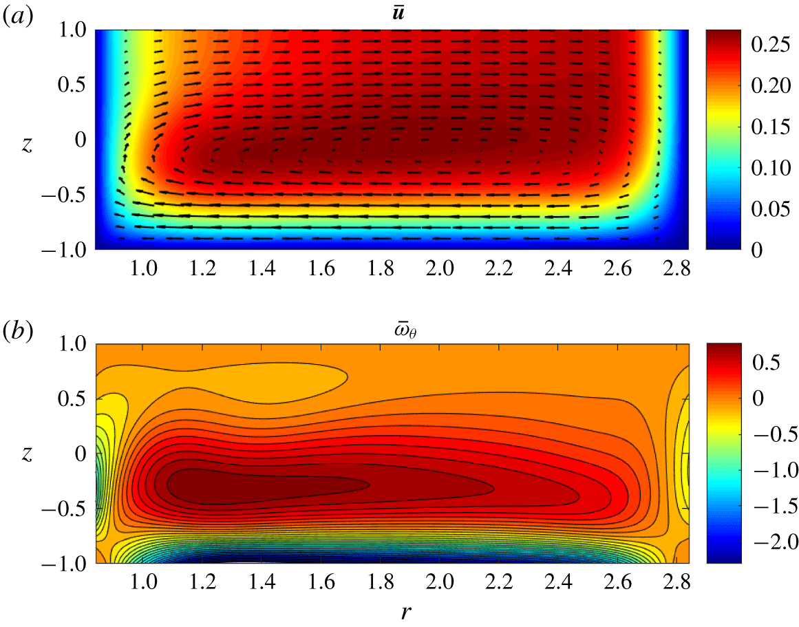
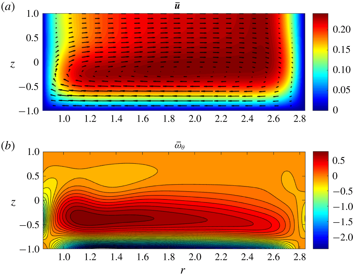
As discussed in Suslov et al. (Reference Suslov, Pérez-Barrera and Cuevas2017) the application of the radial current leads to the appearance of an azimuthal Lorentz force that drives the fluid circumferentially. The appearing centrifugal force then is responsible for the creation of a radial flow component so that the overall flow becomes toroidal. Such a flow was called the Type 1 solution in Suslov et al. (Reference Suslov, Pérez-Barrera and Cuevas2017). It is illustrated in figure 2, where
 $$\begin{eqnarray}\unicode[STIX]{x1D714}_{\unicode[STIX]{x1D703}}=\frac{1}{\unicode[STIX]{x1D716}}\text{D}_{z}u_{r}-\unicode[STIX]{x1D716}\text{D}_{r}u_{z},\end{eqnarray}$$
is the azimuthal component of the vorticity. When the applied current is increased (and so is the value of the Reynolds number  $Re$), the second axisymmetric solution, referred to as Type 2, appears (at some Reynolds number
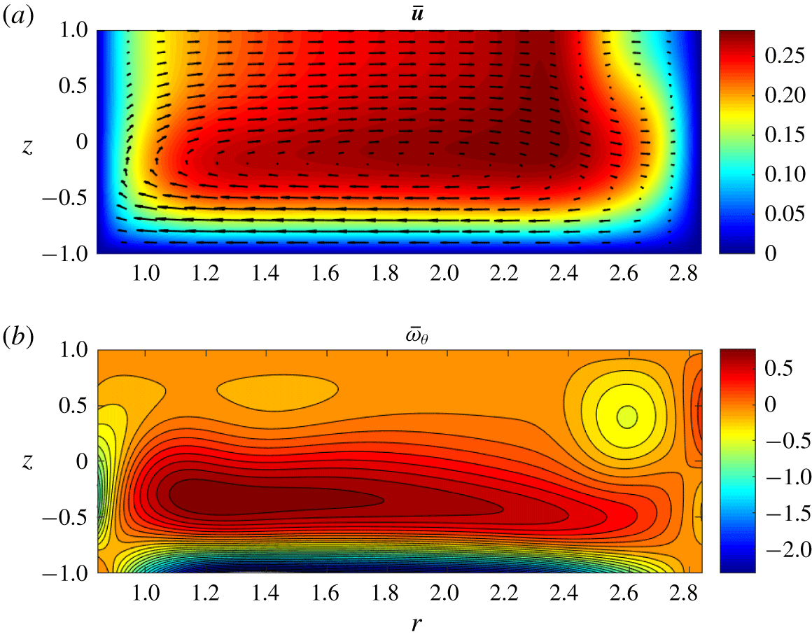
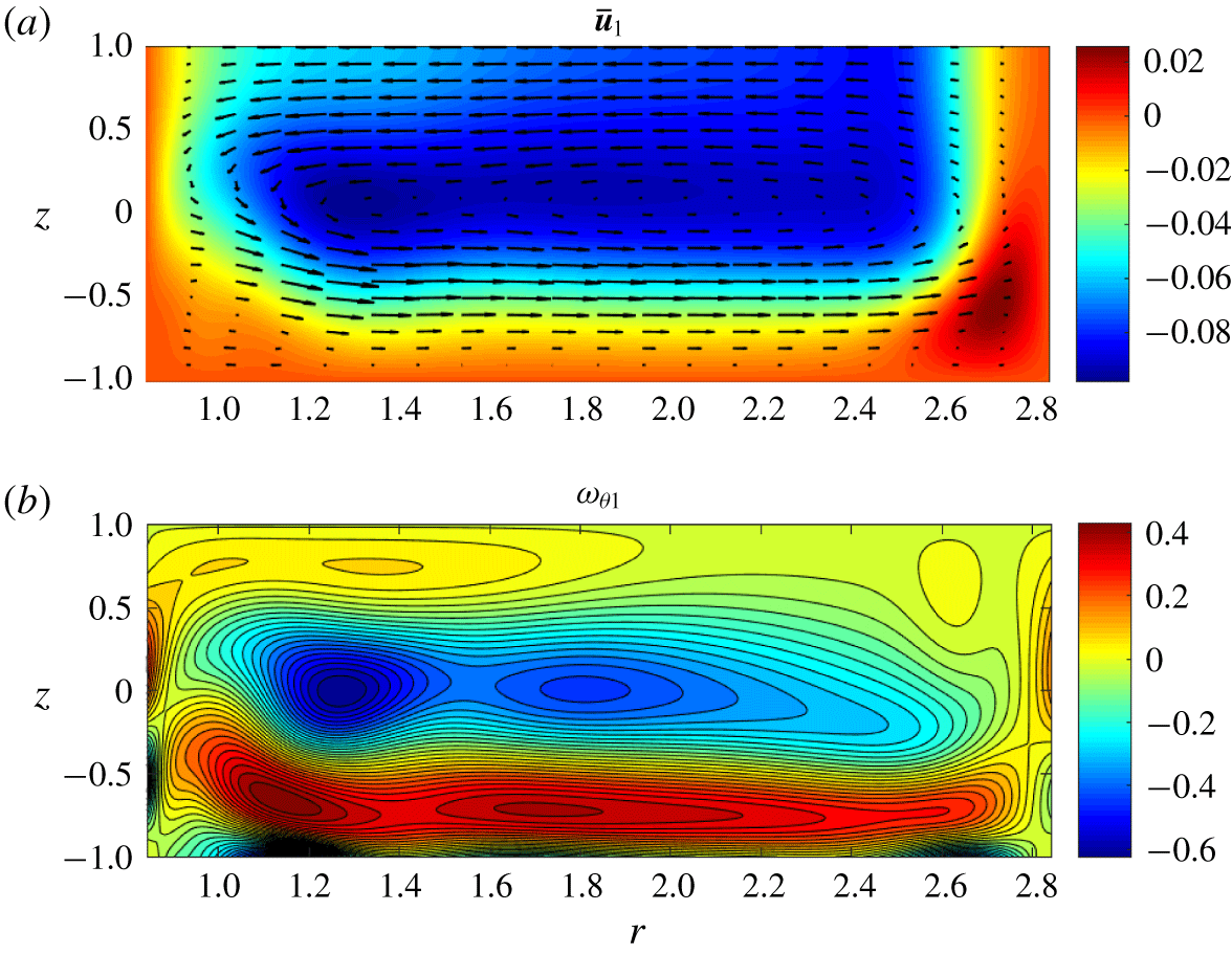
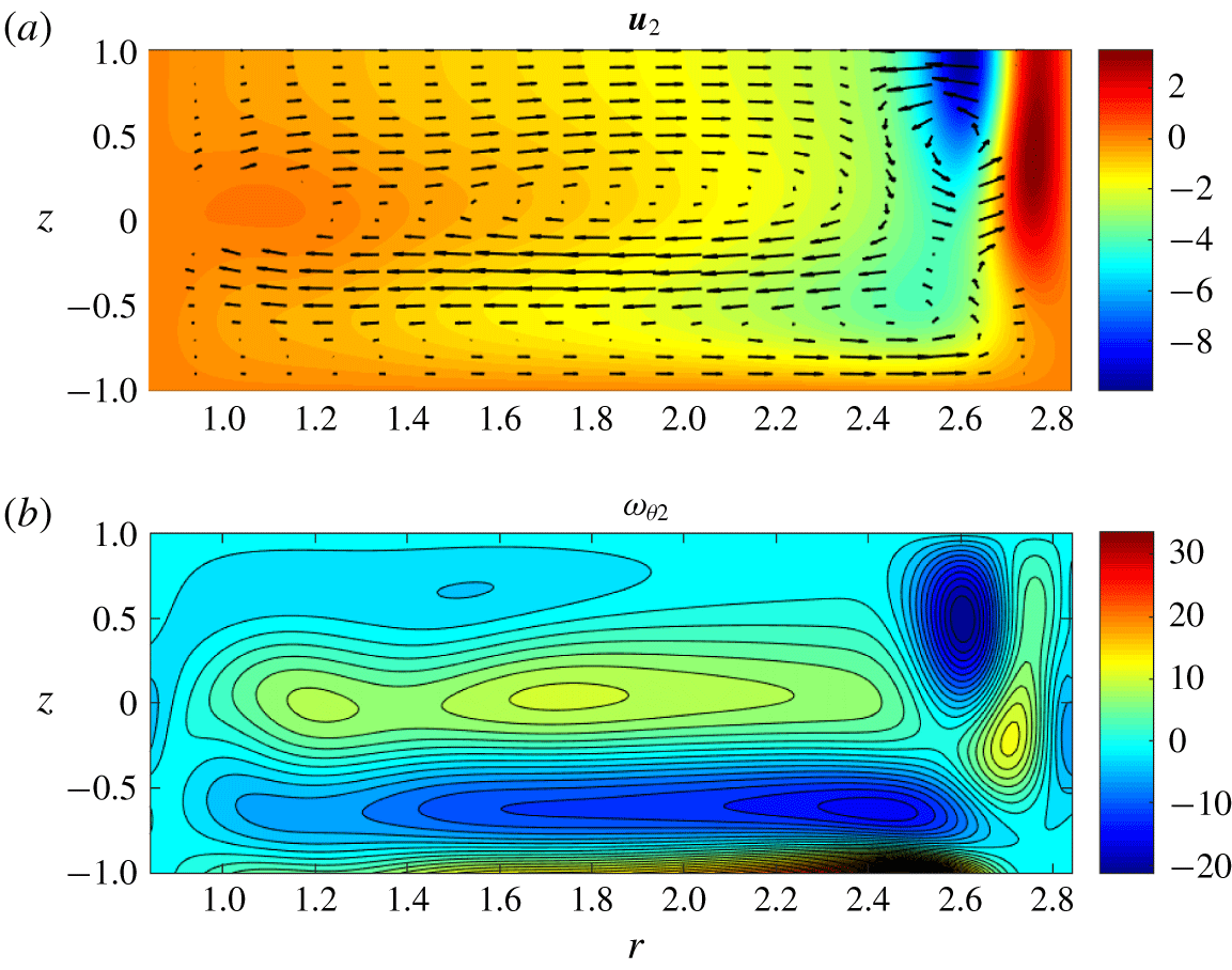
 $Re=Re_{\ast }$). The main feature of this solution, which distinguishes it from its Type 1 counterpart, is the existence of a secondary toroidal structure with fluid counter-rotating in the meridional plane, as illustrated in figure 3. It creates a counter flow near the free surface with a stagnation point some distance away from the outer wall. The Type 1 and 2 solutions can co-exist over a finite range of parameters, i.e. for
 $Re_{\ast }<Re<Re_{\ast \ast }$, but both disappear for
 $Re>Re_{\ast \ast }$. The purpose of the analysis that we undertake next is to quantitatively identify the boundaries of the existence region of these two solutions, to explore their stability and to pinpoint the physical mechanism of the instability leading to the formation of the experimentally observed vortices near the outer cylindrical wall.
Meridional velocity (a) and azimuthal vorticity (b) fields for the Type 1 steady axisymmetric basic flow solution for  $\unicode[STIX]{x1D716}=0.248$,
 $Ha=5.08\times 10^{-3}$ and
 $Re=Re_{\ast }=1032$. The light/red (dark/blue) regions in panel (a) correspond to large (near-zero) values of the azimuthal velocity component
 $u_{\unicode[STIX]{x1D703}}$. The light/red (dark/blue) regions in panel (b) correspond to positive (negative) values of the azimuthal vorticity
 $\unicode[STIX]{x1D714}_{\unicode[STIX]{x1D703}}$.

Same as figure 2 but for the Type 2 basic flow solution.

4 Linearised perturbation equations
We refer to the steady axisymmetric solutions of equations (2.2)–(2.6) with boundary conditions (2.12)–(2.15) reviewed in § 3 as the basic flow and denote them by overbars:  $\bar{\boldsymbol{w}}=[\bar{\unicode[STIX]{x1D719}}(x,z),\bar{u}_{r}(x,z),\bar{u}_{\unicode[STIX]{x1D703}}(x,z),\bar{u}_{z}(x,z),\bar{p}(x,z)]$. We investigate their linear stability with respect to infinitesimal periodic perturbations written in the normal mode form
 $$\begin{eqnarray}[\unicode[STIX]{x1D719}^{\prime }(x,z),u_{r}^{\prime }(x,z),u_{\unicode[STIX]{x1D703}}^{\prime }(x,z),u_{z}^{\prime }(x,z),p^{\prime }(x,z)]\exp (\unicode[STIX]{x1D70E}t+\text{i}m\unicode[STIX]{x1D703})+\text{c.c.},\quad m=0,1,2,\ldots ,\end{eqnarray}$$
where c.c. denotes complex conjugate terms,  $\unicode[STIX]{x1D70E}=\unicode[STIX]{x1D70E}^{R}+\text{i}\unicode[STIX]{x1D70E}^{I}$ is the complex temporal amplification rate and
 $m$ is the azimuthal wavenumber. These perturbations must satisfy the following equations linearised about the basic flow:
 $$\begin{eqnarray}\displaystyle 0 & = & \displaystyle \unicode[STIX]{x1D716}^{2}Ha^{2}B_{z}\frac{\text{i}m}{x+\unicode[STIX]{x1D6FC}}u_{r}^{\prime }+\unicode[STIX]{x1D716}^{2}Ha^{2}\left[B_{r}\text{D}_{z}-B_{z}\text{D}_{x}-\frac{B_{z}}{x+\unicode[STIX]{x1D6FC}}\right]u_{\unicode[STIX]{x1D703}}^{\prime }-\unicode[STIX]{x1D716}^{4}Ha^{2}\frac{\text{i}m}{x+\unicode[STIX]{x1D6FC}}u_{z}^{\prime }\nonumber\\ \displaystyle & & \displaystyle +\,\left[\text{D}_{z}^{2}+\unicode[STIX]{x1D716}^{2}\left(\text{D}_{x}^{2}+\frac{\text{D}_{x}}{x+\unicode[STIX]{x1D6FC}}-\frac{m^{2}}{(x+\unicode[STIX]{x1D6FC})^{2}}\right)\right]\unicode[STIX]{x1D719}^{\prime },\end{eqnarray}$$
 $$\begin{eqnarray}\displaystyle 0 & = & \displaystyle -\unicode[STIX]{x1D70E}u_{r}^{\prime }+\left[\frac{1}{Re}\left(\text{D}_{x}^{2}+\frac{\text{D}_{x}}{x+\unicode[STIX]{x1D6FC}}-\frac{1+m^{2}}{(x+\unicode[STIX]{x1D6FC})^{2}}+\frac{\text{D}_{z}^{2}}{\unicode[STIX]{x1D716}^{2}}\right)-\frac{\text{i}m\bar{u}_{\unicode[STIX]{x1D703}}}{x+\unicode[STIX]{x1D6FC}}-\bar{u}_{r}\text{D}_{x}-\text{D}_{x}\bar{u}_{r}-\bar{u}_{z}\text{D}_{z}\right.\nonumber\\ \displaystyle & & \displaystyle -\,\frac{Ha^{2}B_{z}^{2}}{\unicode[STIX]{x1D716}^{2}Re}\bigg]u_{r}^{\prime }+\frac{2}{x+\unicode[STIX]{x1D6FC}}\left[\bar{u}_{\unicode[STIX]{x1D703}}-\frac{\text{i}m}{Re(x+\unicode[STIX]{x1D6FC})}\right]u_{\unicode[STIX]{x1D703}}^{\prime }-\left[\text{D}_{z}\bar{u}_{r}-\frac{Ha^{2}B_{r}B_{z}}{Re}\right]u_{z}^{\prime }\nonumber\\ \displaystyle & & \displaystyle -\,\frac{\text{D}_{x}}{Fr^{2}}p^{\prime }-\frac{\text{i}mB_{z}}{\unicode[STIX]{x1D716}^{2}Re(x+\unicode[STIX]{x1D6FC})}\unicode[STIX]{x1D719}^{\prime },\end{eqnarray}$$
 $$\begin{eqnarray}\displaystyle 0 & = & \displaystyle -\unicode[STIX]{x1D70E}u_{\unicode[STIX]{x1D703}}^{\prime }+\left[\frac{2\text{i}m}{Re(x+\unicode[STIX]{x1D6FC})^{2}}-\text{D}_{x}\bar{u}_{\unicode[STIX]{x1D703}}-\frac{\bar{u}_{\unicode[STIX]{x1D703}}}{x+\unicode[STIX]{x1D6FC}}\right]u_{r}^{\prime }\nonumber\\ \displaystyle & & \displaystyle +\,\left[\frac{1}{Re}\left(\text{D}_{x}^{2}+\frac{\text{D}_{x}}{x+\unicode[STIX]{x1D6FC}}-\frac{1+m^{2}}{(x+\unicode[STIX]{x1D6FC})^{2}}+\frac{\text{D}_{z}^{2}}{\unicode[STIX]{x1D716}^{2}}\right)-\frac{\text{i}m\bar{u}_{\unicode[STIX]{x1D703}}}{x+\unicode[STIX]{x1D6FC}}-\bar{u}_{r}\text{D}_{x}-\frac{\bar{u}_{r}}{x+\unicode[STIX]{x1D6FC}}-\bar{u}_{z}\text{D}_{z}\right.\nonumber\\ \displaystyle & & \displaystyle -\,\left.\frac{Ha^{2}\left(\unicode[STIX]{x1D716}^{2}B_{r}^{2}+B_{z}^{2}\right)}{\unicode[STIX]{x1D716}^{2}Re}\right]u_{\unicode[STIX]{x1D703}}^{\prime }-\text{D}_{z}\bar{u}_{\unicode[STIX]{x1D703}}u_{z}^{\prime }-\frac{\text{i}m}{Fr^{2}(x+\unicode[STIX]{x1D6FC})}p^{\prime }-\frac{B_{r}\text{D}_{z}-B_{z}\text{D}_{x}}{\unicode[STIX]{x1D716}^{2}Re}\unicode[STIX]{x1D719}^{\prime },\end{eqnarray}$$
 $$\begin{eqnarray}\displaystyle 0 & = & \displaystyle -\unicode[STIX]{x1D70E}u_{z}^{\prime }+\left[\frac{Ha^{2}B_{r}B_{z}}{\unicode[STIX]{x1D716}^{2}Re}-\text{D}_{x}\bar{u}_{z}\right]u_{r}^{\prime }\nonumber\\ \displaystyle & & \displaystyle +\,\left[\frac{1}{Re}\left(\text{D}_{x}^{2}+\frac{\text{D}_{x}}{x+\unicode[STIX]{x1D6FC}}-\frac{m^{2}}{(x+\unicode[STIX]{x1D6FC})^{2}}+\frac{\text{D}_{z}^{2}}{\unicode[STIX]{x1D716}^{2}}\right)-\frac{\text{i}m\bar{u}_{\unicode[STIX]{x1D703}}}{x+\unicode[STIX]{x1D6FC}}-\bar{u}_{r}\text{D}_{x}-\text{D}_{z}\bar{u}_{z}-\bar{u}_{z}\text{D}_{z}\right.\nonumber\\ \displaystyle & & \displaystyle \left.-\,\frac{Ha^{2}B_{r}^{2}}{Re}\right]u_{z}^{\prime }-\frac{\text{D}_{z}}{\unicode[STIX]{x1D716}^{2}Fr^{2}}p^{\prime }+\frac{\text{i}mB_{r}}{\unicode[STIX]{x1D716}^{2}Re(x+\unicode[STIX]{x1D6FC})}\unicode[STIX]{x1D719}^{\prime },\end{eqnarray}$$
 $$\begin{eqnarray}\displaystyle 0 & = & \displaystyle \left[\text{D}_{x}+\frac{1}{x+\unicode[STIX]{x1D6FC}}\right]u_{r}^{\prime }+\frac{\text{i}m}{x+\unicode[STIX]{x1D6FC}}u_{\unicode[STIX]{x1D703}}^{\prime }+\text{D}_{z}u_{z}^{\prime },\end{eqnarray}$$
where  $\text{D}_{x}\equiv \unicode[STIX]{x2202}/\unicode[STIX]{x2202}x$ and
 $\text{D}_{z}\equiv \unicode[STIX]{x2202}/\unicode[STIX]{x2202}z$, with boundary conditions
 $$\begin{eqnarray}\displaystyle & \displaystyle u_{r}^{\prime }=u_{\unicode[STIX]{x1D703}}^{\prime }=u_{z}^{\prime }=0\quad \text{at }z=-1\text{ and at }x=\pm 1, & \displaystyle\end{eqnarray}$$
 $$\begin{eqnarray}\displaystyle & \displaystyle u_{z}^{\prime }=\text{D}_{z}u_{r}^{\prime }=\text{D}_{z}u_{\unicode[STIX]{x1D703}}^{\prime }=0\quad \text{at }z=1, & \displaystyle\end{eqnarray}$$
 $$\begin{eqnarray}\displaystyle \displaystyle \unicode[STIX]{x1D719}^{\prime }=0\quad \text{at }x=\pm 1,\quad \text{D}_{z}\unicode[STIX]{x1D719}^{\prime }=0\quad \text{at }z=-1\text{ and }\text{D}_{z}\unicode[STIX]{x1D719}^{\prime }=-\unicode[STIX]{x1D716}^{2}Ha^{2}B_{r}u_{\unicode[STIX]{x1D703}}^{\prime }\text{at }z=1. & & \displaystyle \nonumber\\ \displaystyle & & \displaystyle\end{eqnarray}$$
Note that for thin layers of a weakly conducting electrolyte  $\unicode[STIX]{x1D716}^{2}Ha^{2}\sim \unicode[STIX]{x1D70E}_{e}h^{3}\sim 10^{-7}$. Thus terms proportional to
 $\unicode[STIX]{x1D716}^{2}Ha^{2}$ in equations (4.2) and (4.9) can be neglected without a significant loss of accuracy. Then, we obtain that the perturbation of the electric potential
 $\unicode[STIX]{x1D719}^{\prime }=0$. Therefore, equation (4.2) decouples from the system, which noticeably reduces the computational cost of the analysis. For this reason, all numerical results presented below are obtained assuming that
 $\unicode[STIX]{x1D719}^{\prime }\equiv 0$.
Note that equations (4.3)–(4.6) with boundary conditions (4.7) and (4.8) can be written in an operator form
 $$\begin{eqnarray}{\mathcal{L}}_{\unicode[STIX]{x1D70E},m;\boldsymbol{P}}\boldsymbol{w}^{\prime }=\mathbf{0},\end{eqnarray}$$
where  $\boldsymbol{w}^{\prime }=[u_{r}^{\prime },u_{\unicode[STIX]{x1D703}}^{\prime },u_{z}^{\prime },p^{\prime }]^{\text{T}}$ and
 $\boldsymbol{P}=(Re,Fr,Ha,\unicode[STIX]{x1D716})$, to be used in § 7.
5 Linear stability results
Linearised perturbation (4.3)–(4.6) form a generalised eigenvalue problem for the complex amplification rate  $\unicode[STIX]{x1D70E}$ that has been solved using a standard Matlab routine eigs. The numerical results have been computed using a grid with
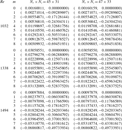
 $N_{r}\times N_{z}=45\times 31$ collocation points in the radial and vertical directions, respectively. As demonstrated by the data in table 1, such a spatial resolution is sufficient to compute eigenvalues
 $\unicode[STIX]{x1D70E}$ with at least 6 significant digits across the parametric range of interest. This enabled us to obtain numerical values of the critical Reynolds numbers with at least 4 significant digits and of the critical non-dimensional depth with at least 3 significant digits, see table 2.
Numerical convergence for leading eigenvalues  $\unicode[STIX]{x1D70E}=(\unicode[STIX]{x1D70E}^{R},\unicode[STIX]{x1D70E}^{I})$ for the Type 2 solution at various Reynolds numbers and for a fixed layer depth
 $h=7.5~\text{mm}$ (
 $\unicode[STIX]{x1D716}=0.248$).

To mimic the experimental procedure while conducting parametric studies we kept the geometry of the problem fixed and varied the Reynolds number. Note that the Froude number is related to the Reynolds number by  $Fr=kRe$, where the proportionality constant
 $k=2\sqrt{2}\unicode[STIX]{x1D707}/(\unicode[STIX]{x1D70C}(R_{2}-R_{1})\sqrt{gh})\sim 3\times 10^{-4}$. The small value of
 $k$ justifies the use of the flat-free-surface approximation in our computations. This scenario corresponds to the variation of an electric current in an otherwise fixed experimental set-up (Pérez-Barrera et al. Reference Pérez-Barrera, Pérez-Espinoza, Ortiz, Ramos and Cuevas2015). The numerical results obtained for this scenario will be discussed first. The experimental variations of the depth of the electrolyte layer and of the strength of the used magnet are accounted for by the corresponding variations of parameters
 $\unicode[STIX]{x1D716}$ and
 $Ha$. These will be discussed in the second half of the current section.
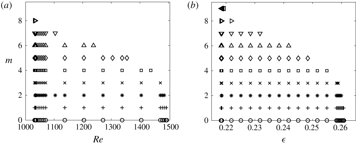
Linear stability diagram for the electrolyte layer placed 6 mm above the disk magnet with  $B_{0}=0.02~\text{T}$: (a) variable current and fixed depth
 $h=7.5~\text{mm}$ (
 $\unicode[STIX]{x1D716}=0.248$,
 $Ha=5.08\times 10^{-3}$); (b) variable depth and fixed current
 $I_{0}=0.2~\text{A}$. Various symbols represent modes with different azimuthal wavenumbers
 $m$.

The typical cumulative stability diagram for the variable-current scenario is shown in figure 4(a). Symbols denote representative parametric points, where the complex amplification rates corresponding to various values of the azimuthal wavenumber  $m$ are found to have positive real parts so that the parametric region containing all the symbols is the linear instability region of the steady axisymmetric basic flow. It is seen from figure 4(a) that, for the chosen combination of geometric and magnetic field parameters, the linear instability is observed only over a finite range of Reynolds numbers (the applied current)
 $Re_{\ast }\leqslant Re\leqslant Re_{\ast \ast }$ with both left and right parametric boundaries being sharply defined (
 $Re_{\ast }\approx 1032$ and
 $Re_{\ast \ast }\approx 1494$ in figure 4a). The maximum azimuthal wavenumber at which the instability can still be observed is
 $m=8$ and it becomes smaller as the value of the Reynolds number (the applied current) increases.
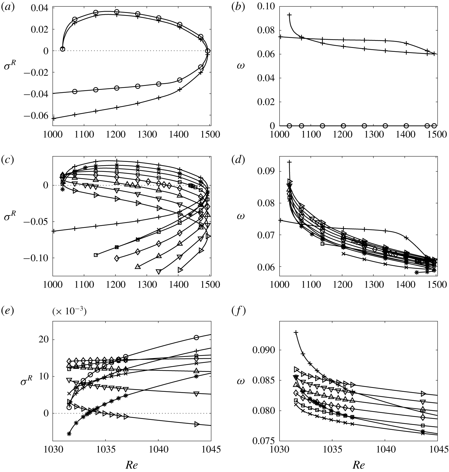
Linear amplification growth rate  $\unicode[STIX]{x1D70E}^{R}$ (a,c,e) and the angular speed
 $\unicode[STIX]{x1D714}=-\unicode[STIX]{x1D70E}^{I}/m$,
 $m\neq 0$ (given that
 $\unicode[STIX]{x1D70E}^{I}=0$ for
 $m=0$ the value of
 $\unicode[STIX]{x1D714}$ is defined to be zero in this case) of the vortex translation (b,d,f) for the stability diagram shown in figure 4 for
 $m=0,1$ (a,b) and
 $m=1,\ldots ,8$ (c–f) (symbols are defined in figure 4). The lower branches of the
 $\unicode[STIX]{x1D70E}^{R}$ curves in panel (c) are truncated at some arbitrary negative values to avoid clutter. The upper branches are shown in full. Panels (e,f) show details near the onset of the Type 2 solution at
 $Re=Re_{\ast }$.

To reveal further features of the observed instability in figure 5 we present real amplification rates  $\unicode[STIX]{x1D70E}^{R}$ and the corresponding angular speeds
 $\unicode[STIX]{x1D714}=-\unicode[STIX]{x1D70E}^{I}/m$ of perturbations for various values of
 $m$ as functions of the Reynolds number. The figure is split into three rows of plots to avoid clutter and clearly show the details. The
 $\unicode[STIX]{x1D70E}^{R}(Re;m)$ curves have a rather peculiar shape of semi-closed loops that we interpret next.
Near the left edge of figure 5(a,c) the leading eigenvalues (that have the largest  $\unicode[STIX]{x1D70E}^{R}$ values for a given set of physical governing parameters for each
 $m$) belong to different branches of the
 $\unicode[STIX]{x1D70E}^{R}$ curves. This is because they correspond to the two distinct axisymmetric basic flow solutions of Types 1 and 2. The eigenvalues corresponding to the Type 2 solutions form the upper branches of the
 $\unicode[STIX]{x1D70E}^{R}$ curves and have positive real parts for
 $m=0,\ldots ,8$ while the real parts of eigenvalues corresponding to the Type 1 solutions remain negative for all wavenumbers
 $m$ (lower branches of the
 $\unicode[STIX]{x1D70E}^{R}$ curves). Therefore, we conclude that only the Type 2 basic flow, and more specifically, the toroidal flow structure existing in the vicinity of the outer wall of the annulus, can lead to the formation of experimentally observed vortices reported in Pérez-Barrera et al. (Reference Pérez-Barrera, Pérez-Espinoza, Ortiz, Ramos and Cuevas2015) and Suslov et al. (Reference Suslov, Pérez-Barrera and Cuevas2017). However, steady Type 2 flows can only exist at sufficiently strong forcing for
 $Re>Re_{\ast }$, where
 $Re_{\ast }$ generally depends on the strength of the magnetic field and the depth of the layer. This is why the upper branches of the
 $\unicode[STIX]{x1D70E}^{R}$ and
 $\unicode[STIX]{x1D714}$ curves do not continue for
 $Re<Re_{\ast }$, see figure 5(a,c,e): the Type 2 axisymmetric basic flow solution, the stability of which they characterise, ceases to exist for
 $Re<Re_{\ast }$. Figure 5(e) demonstrates another experimentally verifiable feature: as the value of the current driving the basic flow (or
 $Re$) is gradually increased, the Type 2 solution appears in an abrupt way. As soon as this happens, it becomes unstable with respect to multiple vortices (corresponding to eigenmodes with
 $m=1$, 3–8, see figure 5e). This is consistent with the experimental photograph shown in figure 17 in our previous publication (Suslov et al. Reference Suslov, Pérez-Barrera and Cuevas2017), where an ink tracer ring evidences the formation of a secondary toroidal structure, which is the feature of the Type 2 solution, with a series of vortices beginning to form along it. Figure 5(f) reveals another noteworthy feature: generally the instability modes corresponding to different wavenumbers
 $m$ are characterised by close but distinct angular wave speeds. The exceptions are modes with
 $m=1$ and 2 that have wave speeds becoming equal to those of other modes at certain values of
 $Re$. Therefore, a resonant interaction between these modes is expected. However, its details cannot be captured within the framework of a linear stability analysis. Quantifying them would require a nonlinear analysis that we leave for a future study.
As  $Re$ (electric current) increases the two types of basic flow continue to exist with Type 1 remaining stable, see the lower branches of the
 $\unicode[STIX]{x1D70E}^{R}$ curves in figure 5, while the stability of Type 2 basic flow depends on
 $m$. Near the onset of the Type 2 flow (
 $Re\gtrsim Re_{\ast }$) the dependence of the flow stability characteristics on
 $m$ is non-monotonic, see the left ends of the upper
 $\unicode[STIX]{x1D70E}^{R}$ curve branches in figure 5(c,e) and numerical values of
 $\unicode[STIX]{x1D70E}^{R}$ listed in tables 1 and 3 for
 $Re=1032$. For larger
 $Re$, the steady Type 2 axisymmetric flow monotonically stabilises with respect to perturbations corresponding to larger azimuthal wavenumbers, see figure 5(a,c). Eventually, at
 $Re_{\ast \ast }\approx 1494$, the distinction between Type 1 and Type 2 solutions (that is the toroidal structure near the outer wall) disappears, see figure 12 and its discussion in § 7.3, and the two branches of the
 $\unicode[STIX]{x1D70E}^{R}$ curves ‘collide’, forming a blunt nose at their right extremes. Beyond this point no steady axisymmetric flow solutions are found, indicating that
 $Re_{\ast \ast }\approx 1494$ is a saddle-node bifurcation point for the steady axisymmetric flow solution. The flow behaviour in the vicinity of this point will be analysed in § 7.
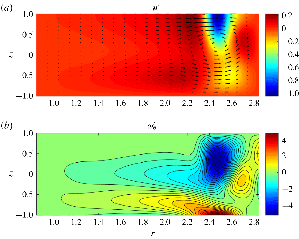
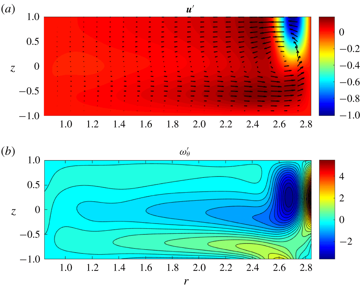
Meridional perturbation velocity (a) and azimuthal vorticity (b) fields corresponding to the azimuthal wavenumber  $m=0$ for the Type 2 steady axisymmetric basic flow solution at
 $\unicode[STIX]{x1D716}=0.248$,
 $Ha=5.08\times 10^{-3}$ and
 $Re=Re_{\ast }=1032$. The light/red (dark/blue) regions in panel (a) correspond to large (near-zero) values of the azimuthal velocity component
 $u_{\unicode[STIX]{x1D703}}^{\prime }$. The light/red (dark/blue) regions in panel (b) correspond to positive (negative) values of the azimuthal vorticity
 $\unicode[STIX]{x1D714}_{\unicode[STIX]{x1D703}}^{\prime }$. The eigenfunctions are normalised so that
 $\max (|u_{r}^{\prime }|,|u_{\unicode[STIX]{x1D703}}^{\prime }|,|u_{z}^{\prime }|)=1$, where the maximum is found of the values at the collocation points.

In figure 6 the typical perturbation velocity and azimuthal vorticity fields in a meridional plane are shown for  $m=0$ (axisymmetric perturbations). The figure demonstrates that the perturbation maximum is located near the corner formed by the free surface and the outer cylinder, as indeed is seen in experiments. The axisymmetric perturbation field has the form of a toroidal structure similar to that existing in the Type 2 basic flow solution. However, in contrast to the basic flow, the flow perturbation velocity field develops an azimuthal jet in the top corner of the annulus near the outer cylinder (see the dark/blue region in the top panel in figure 6). Such a perturbation flow structure, characterised by the co-directed
 $u_{\unicode[STIX]{x1D703}}^{\prime }$ and
 $\unicode[STIX]{x1D714}_{\unicode[STIX]{x1D703}}^{\prime }$ components (the product
 $u_{\unicode[STIX]{x1D703}}^{\prime }\unicode[STIX]{x1D714}_{\unicode[STIX]{x1D703}}^{\prime }$ is positive), is very robust. It is preserved for all growing azimuthally periodic perturbations with
 $m=1,\ldots ,8$ (not shown explicitly due to the qualitative similarity of the meridional perturbation fields).
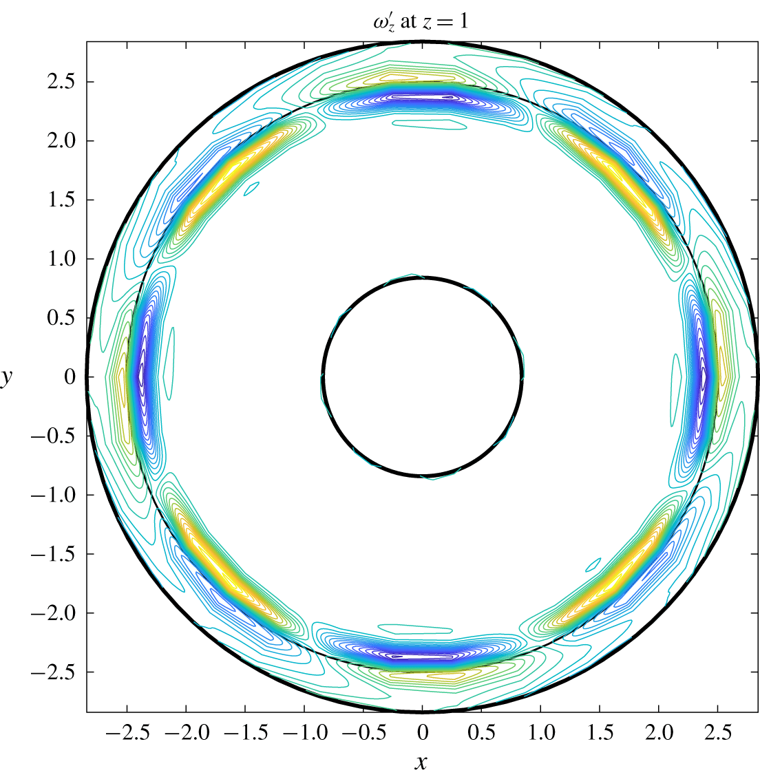
The vertical perturbation vorticity component  $\unicode[STIX]{x1D714}_{z}^{\prime }=\text{D}_{r}u_{\unicode[STIX]{x1D703}}^{\prime }+u_{\unicode[STIX]{x1D703}}^{\prime }/r$ at the free surface (
 $z=1$) for the same parameters as in figure 6 but for
 $m=4$. The solid circular line represents the location on the free surface, where the local basic flow velocity component
 $u_{\unicode[STIX]{x1D703}}$ is equal to the wave speed
 $\unicode[STIX]{x1D714}r$ (the angular speed
 $\unicode[STIX]{x1D714}$ is given in figure 5b,d,f).

The main difference between the perturbation fields corresponding to  $m=0$ and
 $m\neq 0$ is that, for periodic perturbations, the axisymmetric toroidal jet breaks into cells corresponding to the vortices illustrated in figure 7. The condition
 $u_{\unicode[STIX]{x1D703}}^{\prime }\unicode[STIX]{x1D714}_{\unicode[STIX]{x1D703}}^{\prime }>0$ is satisfied within individual cells. The cell centres drift with the speed of the local basic flow along the circular line in figure 7. This line separates regions with the opposite
 $z$ vorticity component within each cell. As follows from figure 5(b,d), the axisymmetric instability structures with
 $m=0$ remain stationary while the non-zero angular speeds of the periodic perturbation corresponding to wavenumbers
 $m=1,\ldots ,8$ have very close values and thus the corresponding vortex systems are expected to interact with each other, forming the beating patterns seen experimentally. However, such an interaction cannot be accounted for within the framework of a linear analysis alone and requires nonlinear consideration that we plan for future studies.
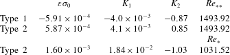
From a linear stability point of view, we can consider each instability mode characterised by wavenumber  $m$ individually and determine the critical values of the parameters at which they are expected to arise; an example of such data is given in table 2. The Type 2 basic flow solutions computed for
 $\unicode[STIX]{x1D716}=0.248$ (
 $h=7.5~\text{mm}$) become unstable with respect to various modes corresponding to
 $m=0,\ldots ,8$ for Reynolds numbers ranging between the values specified in rows 2 and 3. The table data contain quantitative information for the left and right limits of the instability region shown in figure 4(a). For
 $m=0$, 1, and 3–8 the values of the Reynolds number, at which the corresponding unstable modes are first detected, coincide with
 $Re_{\ast }$ at which the Type 2 solution itself first occurs. Therefore, the Type 2 solution is unstable with respect to these modes from its very onset. Only the
 $m=2$ mode experiences transition to instability at a slightly larger value of the Reynolds number. The critical values of the Reynolds number,
 $Re_{c}$, at which the individual modes stabilise as
 $Re$ increases, decrease monotonically with the growth of wavenumber
 $m$. Thus, progressively faster flows are expected to develop fewer vortices.
The critical values  $Re_{c}$ and
 $\unicode[STIX]{x1D716}_{c}$ for linear instability of the Type 2 axisymmetric steady basic flow solution at
 $B_{0}=0.02~\text{T}$ for various values of the azimuthal wavenumber
 $m$. Rows 2 and 3: fixed
 $h=7.5~\text{mm}$ (
 $\unicode[STIX]{x1D716}=0.248$,
 $Ha=5.08\times 10^{-3}$), variable
 $I_{0}$; rows 4 and 5: fixed
 $I_{0}=0.2~\text{A}$, variable
 $h$.

The second experimental scenario corresponds to the exploration of flow structures arising in a variable-depth electrolyte layer placed in a magnetic field created by a fixed magnet ( $B_{0}=\text{const}.$) and subject to a fixed radial current (
 $I_{0}$) (Pérez-Barrera et al. Reference Pérez-Barrera, Pérez-Espinoza, Ortiz, Ramos and Cuevas2015). In this case, all non-dimensional governing parameters change as functions of
 $\unicode[STIX]{x1D716}$ according to (2.1) and (2.11) (which is less convenient from the point of view of a theoretical parametric study). However, there are two parametric invariants in this scenario,
 $$\begin{eqnarray}\displaystyle & \displaystyle {\mathcal{I}}_{1}\equiv \frac{Ha}{Re}=\frac{4\unicode[STIX]{x03C0}\unicode[STIX]{x1D707}\sqrt{\unicode[STIX]{x1D707}\unicode[STIX]{x1D70E}_{e}}}{\unicode[STIX]{x1D70C}I_{0}\ln (R_{2}/R_{1})}\quad \text{and} & \displaystyle\end{eqnarray}$$
 $$\begin{eqnarray}\displaystyle & \displaystyle {\mathcal{I}}_{2}\equiv \frac{\unicode[STIX]{x1D716}}{Re}=\frac{8\unicode[STIX]{x03C0}\unicode[STIX]{x1D707}^{2}}{\unicode[STIX]{x1D70C}B_{0}I_{0}(R_{2}-R_{1})\ln (R_{2}/R_{1})}. & \displaystyle\end{eqnarray}$$
The numerical data shown in figure 4(b) and given in rows 4 and 5 in table 2 are obtained for fixed electric current  $I_{0}=0.2$ A and magnetic field
 $B_{0}=0.02$ T that correspond to the invariant values
 ${\mathcal{I}}_{1}=3.80\times 10^{-6}$ and
 ${\mathcal{I}}_{2}=1.86\times 10^{-4}$. We also note that
 $$\begin{eqnarray}\frac{Fr^{2}}{Re}=\frac{B_{0}I_{0}\ln (R_{2}/R_{1})}{\unicode[STIX]{x1D70C}g(R_{2}-R_{1})^{2}}=1.60\times 10^{-4},\end{eqnarray}$$
indicating that the flat-free-surface approximation remains reasonably accurate in the considered regimes. These data enable us to make several noteworthy conclusions.
The instability region for a variable-depth electrolyte layer shown in panel (b) in figure 4 has a shape qualitatively similar to that for the constant-depth layer presented in panel (a). It has a sharp left edge, signifying that the Type 2 basic flow solution can only exist in sufficiently thick layers when the current is fixed. The right edge of the instability region is curved, indicating that various vortex modes have different instability ranges. The general trend is that thicker layers can only support instability patterns with fewer vortices. This is consistent with the experimental observations reported in Pérez-Barrera et al. (Reference Pérez-Barrera, Pérez-Espinoza, Ortiz, Ramos and Cuevas2015). The maximum number of vortices that can be observed at  $I_{0}=0.2~\text{A}$ and
 $B_{0}=0.02~\text{T}$ is nine. The Reynolds number ranges for instabilities with different wavenumbers are given in rows 4 and 5 of table 2. Computations show that the widest instability ranges always correspond to
 $m=0$. Such axisymmetric modes also have the largest maximum amplification rate
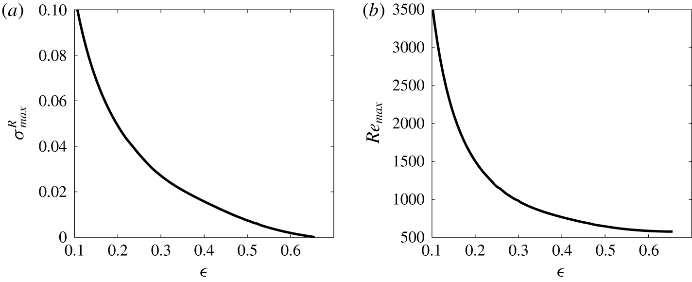
 $\unicode[STIX]{x1D70E}_{max}^{R}$ among all other modes. The value of
 $\unicode[STIX]{x1D70E}_{max}^{R}$ is shown as a function of
 $\unicode[STIX]{x1D716}$ in figure 8(a) and the corresponding Reynolds number,
 $Re_{max}$, at which it occurs in layers of various depths is depicted in figure 8(b). Both quantities monotonically decrease with the layer depth, reaching
 $\unicode[STIX]{x1D70E}_{max}^{R}\approx 0$ at
 $(\unicode[STIX]{x1D716},Re_{max})\approx (0.656,576)$.
(a) The maximum linear amplification rate  $\unicode[STIX]{x1D70E}_{max}^{R}$ and (b) the value of Reynolds number
 $Re_{max}$ at which it is observed as functions of the non-dimensional layer thickness
 $\unicode[STIX]{x1D716}$ for
 $m=0$.

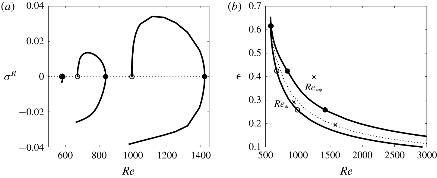
In order to reveal what happens as the layer depth increases, we inspect figure 9(a), where the  $\unicode[STIX]{x1D70E}^{R}$ curves corresponding to
 $m=0$ are shown for progressively thicker electrolyte layers. Similar to figure 5, the segments of the curves with
 $\unicode[STIX]{x1D70E}^{R}<0$ below points marked by filled circles correspond to the stable Type 1 basic flow while the
 $\unicode[STIX]{x1D70E}^{R}>0$ curve segments between the empty and filled circles correspond to the unstable axisymmetric Type 2 solutions. As the layer thickness increases, the curves shift towards smaller values of the Reynolds number and the existence range of the Type 2 solution (between the open and filled circles) shrinks, until it disappears at
 $\unicode[STIX]{x1D716}\approx 0.656$ (a saddle-node bifurcation). By tracing the location of points marked by the empty and filled circles in figure 9(a) for various values of
 $\unicode[STIX]{x1D716}$, we construct the overall stability diagram shown in figure 9(b). The vortices superposed on the toroidal axisymmetric Type 2 basic flow are expected to be observed in a parametric region between the
 $Re_{\ast }$ and
 $Re_{\ast \ast }$ curves. This conclusion is in agreement with experimental data reported previously (for an annulus of slightly different geometry) by Pérez-Barrera et al. (Reference Pérez-Barrera, Pérez-Espinoza, Ortiz, Ramos and Cuevas2015), see the crosses in figure 9(b). Below the
 $Re_{\ast }$ curve, steady axisymmetric Type 1 flow is expected to exist. The experimental observations of Pérez-Barrera et al. (Reference Pérez-Barrera, Pérez-Espinoza, Ortiz, Ramos and Cuevas2015) indicate that flow above the
 $Re_{\ast \ast }$ curve still contains multiple unsteady vortices, see the cross at
 $(\unicode[STIX]{x1D716},Re)\approx (0.4,1250)$ in figure 9(b). The analysis of solutions existing above the
 $Re_{\ast \ast }$ curve (beyond the saddle-node bifurcation) will be developed in § 7.
(a) The  $\unicode[STIX]{x1D70E}^{R}(Re)$ curves for
 $m=0$ and (from right to left)
 $\unicode[STIX]{x1D716}=0.258$, 0.424 and 0.616; (b) the existence region between the
 $Re_{\ast }$ (open circles) and
 $Re_{\ast \ast }$ (filled circles) curves of the Type 2 steady axisymmetric flow solutions corresponding to the
 $\unicode[STIX]{x1D70E}^{R}>0$ ranges in panel (a). The dotted line in panel (b) corresponds to the solid line in figure 8(b). The crosses show the experimental data for vortex onset reported by Pérez-Barrera et al. (Reference Pérez-Barrera, Pérez-Espinoza, Ortiz, Ramos and Cuevas2015).

The results of a linear stability analysis indicate that such vortices can in principle exist in very thin layers. However, the corresponding values of the Reynolds number increase quickly as the depth of the layer decreases. This is because, in thin layers, the relative role of viscous dissipation at the stationary solid bottom strengthens and a much larger electric current is required to drive the fluid. As follows from figure 9(b), the instability in such thin layers is expected to occur at  $Re>2500$, which would correspond to progressively larger values of the Froude number, see (5.3). The shape of the free surface can noticeably deviate from flat in such regimes. For example, following Suslov et al. (Reference Suslov, Pérez-Barrera and Cuevas2017), we estimate that at
 $\unicode[STIX]{x1D716}=0.1$ the vortex instability would set in when the free-surface deformation reaches more than 10 % of the layer thickness, which is not taken into account in the computational model used here. While the qualitative structure of the flow in these regimes is expected to be similar to that predicted by our current model (a similar conclusion has been made in Yang et al. (Reference Yang, Delbende, Fraigneau and Witkowski2019)), the quantitative errors are not likely to remain negligible. Experimental observations of a vortex instability in very thin layers are also unlikely to succeed because the strong electric current flowing through the layer would cause intensive electrolysis at the surface of copper electrodes. This would produce hydrogen bubbles of a size comparable with the layer thickness that would significantly vary the physical boundary conditions and uncontrollably distort the flow velocity profile. Thus, when constructing figure 9(b), we did not perform stability computations for
 $\unicode[STIX]{x1D716}\lesssim 0.1$.
6 Perturbation energy consideration
In order to gain an insight into the mechanisms driving the instability of steady axisymmetric basic flow, we multiply equations (4.3)–(4.5) by the complex conjugate perturbation velocity components  $(u_{r}^{\ast },u_{\unicode[STIX]{x1D703}}^{\ast },u_{z}^{\ast })$, respectively, integrate (by parts when necessary) over the meridional cross-section using the corresponding boundary conditions for velocities and the continuity equation to eliminate pressure and obtain the following equation representing the conservation of mechanical energy in the system:
 $$\begin{eqnarray}\unicode[STIX]{x1D70E}\unicode[STIX]{x1D6F4}_{k}=\unicode[STIX]{x1D6F4}_{Ha}+\unicode[STIX]{x1D6F4}_{bf}+\unicode[STIX]{x1D6F4}_{c}+\unicode[STIX]{x1D6F4}_{vis},\end{eqnarray}$$
where
 $$\begin{eqnarray}\displaystyle & \displaystyle \unicode[STIX]{x1D6F4}_{k}=\int _{-1}^{1}\int _{-1}^{1}(x+\unicode[STIX]{x1D6FC})E_{k}\text{d}x\,\text{d}z,\quad \unicode[STIX]{x1D6F4}_{Ha}=\int _{-1}^{1}\int _{-1}^{1}(x+\unicode[STIX]{x1D6FC})E_{Ha}\text{d}x\,\text{d}z, & \displaystyle \nonumber\\ \displaystyle & \displaystyle \unicode[STIX]{x1D6F4}_{bf}=\int _{-1}^{1}\int _{-1}^{1}(x+\unicode[STIX]{x1D6FC})E_{bf}\text{d}x\,\text{d}z,\quad \unicode[STIX]{x1D6F4}_{c}=\int _{-1}^{1}\int _{-1}^{1}(x+\unicode[STIX]{x1D6FC})E_{c}\text{d}x\,\text{d}z, & \displaystyle \nonumber\\ \displaystyle & \displaystyle \unicode[STIX]{x1D6F4}_{vis}=\int _{-1}^{1}\int _{-1}^{1}(x+\unicode[STIX]{x1D6FC})E_{vis}\text{d}x\,\text{d}z & \displaystyle \nonumber\end{eqnarray}$$
and
 $$\begin{eqnarray}\displaystyle & \displaystyle E_{k}=|u_{r}^{\prime }|^{2}+|u_{\unicode[STIX]{x1D703}}^{\prime }|^{2}+\unicode[STIX]{x1D716}^{2}|u_{z}^{\prime }|^{2}, & \displaystyle\end{eqnarray}$$
 $$\begin{eqnarray}\displaystyle & \displaystyle E_{Ha}=-\frac{Ha^{2}}{\unicode[STIX]{x1D716}^{2}Re}\left(B_{z}^{2}|u_{r}^{\prime }|^{2}+(\unicode[STIX]{x1D716}^{2}B_{r}^{2}+B_{z}^{2})|u_{\unicode[STIX]{x1D703}}^{\prime }|^{2}-2\unicode[STIX]{x1D716}^{2}B_{r}B_{z}\text{Re}\{u_{\unicode[STIX]{x1D703}}^{\prime }u_{z}^{\ast }\}+\unicode[STIX]{x1D716}^{4}B_{r}^{2}|u_{z}^{\prime }|^{2}\right), & \displaystyle\end{eqnarray}$$
 $$\begin{eqnarray}\displaystyle E_{bf} & = & \displaystyle -\bigg[u_{r}^{\ast }(\bar{u}_{r}\text{D}_{x}u_{r}^{\prime }+u_{r}^{\prime }\text{D}_{x}\bar{u}_{r}+\bar{u}_{z}\text{D}_{z}u_{r}^{\prime }+u_{z}^{\prime }\text{D}_{z}\bar{u}_{r})+u_{\unicode[STIX]{x1D703}}^{\ast }(\bar{u}_{z}\text{D}_{z}u_{\unicode[STIX]{x1D703}}^{\prime }+u_{z}^{\prime }\text{D}_{z}\bar{u}_{\unicode[STIX]{x1D703}})\nonumber\\ \displaystyle & & \displaystyle +\,\unicode[STIX]{x1D716}^{2}u_{z}^{\ast }(\bar{u}_{r}\text{D}_{x}u_{z}^{\prime }+u_{r}^{\prime }\text{D}_{x}\bar{u}_{z}+\bar{u}_{z}\text{D}_{z}u_{z}^{\prime }+u_{z}^{\prime }\text{D}_{z}\bar{u}_{z})\nonumber\\ \displaystyle & & \displaystyle +\,\frac{\text{i}m\bar{u}_{\unicode[STIX]{x1D703}}}{x+\unicode[STIX]{x1D6FC}}(|u_{r}^{\prime }|^{2}+|u_{\unicode[STIX]{x1D703}}^{\prime }|^{2}+\unicode[STIX]{x1D716}^{2}|u_{z}^{\prime }|^{2})\bigg],\end{eqnarray}$$
 $$\begin{eqnarray}\displaystyle & \displaystyle E_{c}=\frac{\bar{u}_{\unicode[STIX]{x1D703}}(2u_{r}^{\ast }u_{\unicode[STIX]{x1D703}}^{\prime }-u_{r}^{\prime }u_{\unicode[STIX]{x1D703}}^{\ast })-\bar{u}_{r}|u_{\unicode[STIX]{x1D703}}^{\prime }|^{2}}{x+\unicode[STIX]{x1D6FC}}-u_{\unicode[STIX]{x1D703}}^{\ast }(\bar{u}_{r}\text{D}_{x}u_{\unicode[STIX]{x1D703}}^{\prime }+u_{r}^{\prime }\text{D}_{x}\bar{u}_{\unicode[STIX]{x1D703}}), & \displaystyle\end{eqnarray}$$
 $$\begin{eqnarray}\displaystyle E_{vis} & = & \displaystyle -\frac{1}{Re}\left[\frac{(1+m^{2})(|u_{r}^{\prime }|^{2}+|u_{\unicode[STIX]{x1D703}}^{\prime }|^{2})+\unicode[STIX]{x1D716}^{2}m^{2}|u_{z}^{\prime }|^{2}}{(x+\unicode[STIX]{x1D6FC})^{2}}\right.\nonumber\\ \displaystyle & & \displaystyle +\,|\text{D}_{x}u_{r}^{\prime }|^{2}+|\text{D}_{x}u_{\unicode[STIX]{x1D703}}^{\prime }|^{2}+\unicode[STIX]{x1D716}^{2}|\text{D}_{x}u_{z}^{\prime }|^{2}\nonumber\\ \displaystyle & & \displaystyle \left.+\,\frac{1}{\unicode[STIX]{x1D716}^{2}}(|\text{D}_{z}u_{r}^{\prime }|^{2}+|\text{D}_{z}u_{\unicode[STIX]{x1D703}}^{\prime }|^{2}+\unicode[STIX]{x1D716}^{2}|\text{D}_{z}u_{z}^{\prime }|^{2})+\frac{4m}{(x+\unicode[STIX]{x1D6FC})^{2}}\text{Im}\{u_{r}^{\prime }u_{\unicode[STIX]{x1D703}}^{\ast }\}\right].\end{eqnarray}$$
The above expressions represent easily identifiable physical characteristics and influences. Namely,  $E_{k}$ is real, positively defined and measures the perturbation kinetic energy;
 $E_{Ha}$ and
 $E_{bf}$ represent the electromagnetic effects and the interaction of perturbations with the basic flow (via non-radial shear), respectively;
 $E_{c}$ characterises the effects of curvature and radial shear and includes terms responsible for Rayleigh centrifugal destabilisation (Rayleigh Reference Rayleigh1916) (recollect that Rayleigh inviscid centrifugal instability condition for unidirectional rotational flow is
 $(\unicode[STIX]{x2202}/\unicode[STIX]{x2202}r)(ru_{\unicode[STIX]{x1D703}})<0$ (Greenspan Reference Greenspan1968; Suslov et al. Reference Suslov, Pérez-Barrera and Cuevas2017), which is related to radial shear). The real-valued
 $E_{vis}$ is the measure of viscous dissipation.
For axisymmetric perturbations with  $m=0$,
 $E_{vis}$ is negatively defined. Furthermore, our computations show that it remains negative for
 $m\neq 0$. Since eigenfunctions of a linearised perturbation problem are defined up to an arbitrary multiplicative constant, without loss of generality, we scale them in such a way that
 $\unicode[STIX]{x1D6F4}_{vis}\equiv -1$, so that the strength of all other effects is measured relative to that of viscous dissipation.
Equation (6.1) is an integral form of the linearised perturbation equations that enables one to conveniently and unambiguously discriminate between stabilising and destabilising physical influences: only mechanisms corresponding to terms on the right-hand side of (6.1) that have positive real parts can lead to instability. Since only  $E_{bf}$ and
 $E_{c}$ can assume complex values, and thus determine the non-zero perturbation frequency
 $\unicode[STIX]{x1D70E}^{I}$, we conclude that circumferential translation of vortical instability structures is completely due to the influence of the basic flow and inertial effects associated with the curvature of fluid trajectories.
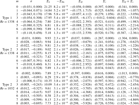
The integral perturbation energy values for linear instability of the Type 1 and Type 2 axisymmetric steady basic flow solutions at  $B_{0}=0.02~\text{T}$ for various values of the azimuthal wavenumber
 $m$ and
 $h=7.5~\text{mm}$ (
 $\unicode[STIX]{x1D716}=0.248$,
 $Ha=5.08\times 10^{-3}$).

The typical numerical values of terms entering (6.1) are listed in table 3. These data enable us to make several conclusions about the physical nature of the detected instabilities. The perturbation kinetic energy values for the Type 1 solution suggest that, even though all leading disturbance modes decay, they belong to two different groups characterised by small and large wavenumbers  $m$. While not given here explicitly, the meridional eigenmode field plots show that, at small
 $m$, the perturbations are located predominantly in the boundary layer near the inner cylinder. The destabilising influence of centrifugal effects decreases with
 $m$ and becomes negative at
 $m=3$. Thus, for larger wavenumbers, the least stable eigenmode fields shift toward the outer wall where the centrifugal effect is much stronger, although still insufficient to destabilise the Type 1 flow. Such a localisation of disturbance fields will be discussed in more detail in the context of the Type 2 flows below.
The Lorentz force that drives the primary flow makes virtually no contribution to the development of the instability: while  $\unicode[STIX]{x1D6F4}_{Ha}$ remains negative and thus stabilising for both Type 1 and 2 solutions, its magnitude is many orders of magnitude smaller than that of the other terms. Centrifugal and radial shear effects are strictly destabilising and supply most of the energy for instability. The contribution of basic flow (non-radial shear) to the overall perturbation energy balance varies with the type of basic axisymmetric flow and Reynolds number. It plays mostly a stabilising role (
 $\text{Re}\{\unicode[STIX]{x1D6F4}_{bf}\}<0$) for the Type 1 solution. However, near the onset of the Type 2 flow (at
 $Re_{\ast }=1032$) it is destabilising and supplies approximately 30 % of the perturbation energy. With the increase of Reynolds number its share drastically reduces in favour of
 $E_{c}$ and even becomes negative at larger wavenumbers. This confirms the hypothesis formulated in Suslov et al. (Reference Suslov, Pérez-Barrera and Cuevas2017) that, in our set-up, the main mechanism leading to the formation of vortices is of centrifugal Rayleigh (Rayleigh Reference Rayleigh1916) type. This is in contrast to experiments reviewed by Dolzhanskii et al. (Reference Dolzhanskii, Krymov and Manin1990), where Kelvin–Helmholtz-type or, more precisely, shear instability, was observed away from cylindrical walls at the location corresponding to the inflection point of the flow velocity profile. Such an azimuthal velocity profile was created there by reversing the direction of the applied vertical magnetic field (and thus of the Lorentz force driving the fluid in opposite directions) in the middle of the channel. In our set-up, the Lorentz force acts in the same azimuthal direction, so that no flow reversal occurs, and the instability arises in the viscous boundary layer near the outer cylindrical wall rather than in the middle of a fluid layer. Therefore, the destabilising effects in our configuration necessarily differ from those discussed by Dolzhanskii et al. (Reference Dolzhanskii, Krymov and Manin1990).
At relatively large Reynolds numbers (see data for  $Re=1338$ in table 3), when the instability is strongly dominated by centrifugal effects, the kinetic energy of perturbations (
 $E_{k}$) decreases relative to viscous dissipation as the wavenumber
 $m$ increases. This is expected, as the larger the wavenumber the smaller the size of the individual vortices and the more densely they are packed in the flow domain. Therefore, they experience stronger dissipation due to friction, which eventually leads to the disappearance of smaller vortices, the effect manifested by increasingly more negative values of the real amplification rate
 $\unicode[STIX]{x1D70E}^{R}$ of the disturbances; see the second column in table 3. However, for smaller Reynolds numbers (see data for
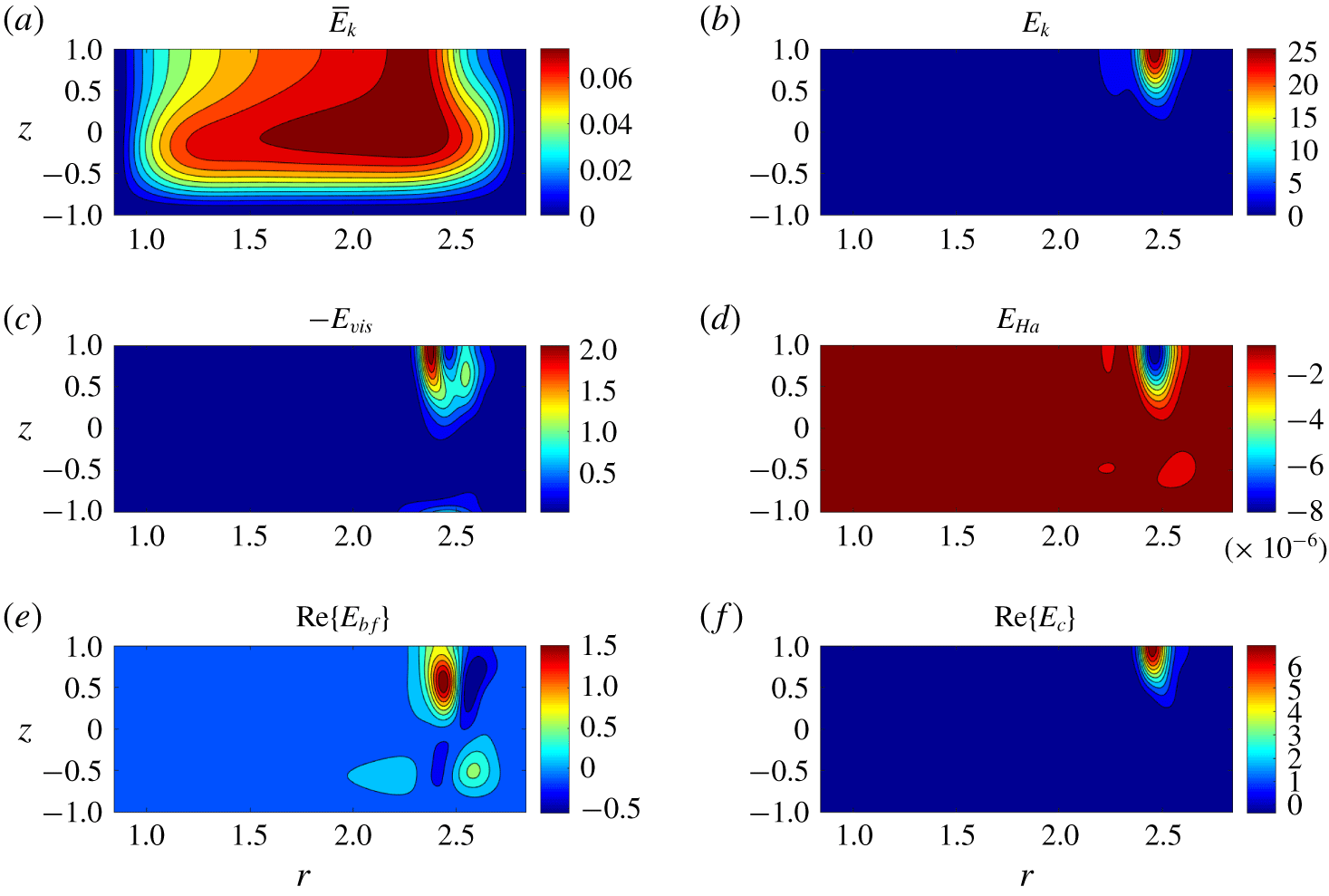
 $Re=1032$ in table 3) the dependence of the perturbation kinetic energy on wavenumber is not monotonic. This is likely to be due to a stronger relative influence of disturbance structures, other than main vortices, existing in slower basic flows. To demonstrate this, in figure 10 we present typical spatial distributions of perturbation energy integrands.
Meridional distributions of the basic flow kinetic energy  $\bar{E}_{k}=\bar{u}_{r}^{2}+\bar{u}_{\unicode[STIX]{x1D703}}^{2}+\unicode[STIX]{x1D716}^{2}\bar{u}_{z}^{2}$ and various perturbation energy integrands given by expressions (6.2)–(6.6) for the Type 2 basic flow solution with
 $m=4$ for the same parameters as in figures 6 and 7. The integrands are normalised so that
 $\unicode[STIX]{x1D6F4}_{vis}=-1$.

Figure 10 demonstrates that, while the basic flow kinetic energy  $\bar{E}_{k}=\bar{u}_{r}^{2}+\bar{u}_{\unicode[STIX]{x1D703}}^{2}+\unicode[STIX]{x1D716}^{2}\bar{u}_{z}^{2}$ is distributed throughout the bulk of the electrolyte layer, the perturbations leading to the formation of vortices are very strongly localised near the outer top corner of the meridional cross-section (as mentioned earlier in this section, a similar localisation of perturbation fields is detected for the Type 1 flows at large wavenumbers even though it does not lead to the formation of vortices there). Comparing distributions of
 $\bar{E}_{k}$ and
 $E_{k}$, we note that vortices are formed in the region where the basic flow is less energetic, and their occurrence reduces the kinetic energy deficit there. The vortical structures are rather shallow and are fully contained in the upper half-layer. The shown distribution of
 $\bar{E}_{k}$ indicates that the thickness of boundary layers at both inner and outer cylindrical surfaces and thus the magnitudes of the radial velocity gradients
 $\left|\unicode[STIX]{x2202}\bar{u}_{\unicode[STIX]{x1D703}}/\unicode[STIX]{x2202}r\right|$ there are similar (see also discussion in Suslov et al. Reference Suslov, Pérez-Barrera and Cuevas2017). Despite this fact, the instability develops only in the vicinity of the outer electrode, where the Rayleigh criterion
 $(\unicode[STIX]{x2202}/\unicode[STIX]{x2202}r)(r\bar{u}_{\unicode[STIX]{x1D703}})<0$ is satisfied, which once again confirms the centrifugal rather than shear nature of the instability. As mentioned in the previous paragraph, the distribution of a non-radial shear (
 $E_{bf}$) indicates that, indeed, it is less localised and is associated with structures other than main vortices, in particular, with the boundary layer in the bottom corner near the outer electrode. No instability structures exist near the inner cylindrical boundary.
Finally, we note that the balance between the imaginary parts of  $\unicode[STIX]{x1D6F4}_{bf}$ and
 $\unicode[STIX]{x1D6F4}_{c}$ determines
 $\unicode[STIX]{x1D70E}^{I}$ and thus defines the vortex angular translation speed
 $\unicode[STIX]{x1D714}=-\unicode[STIX]{x1D70E}^{I}/m$. The data in table 3 show that this vortex characteristic is predominantly determined by the basic flow contribution
 $\text{Im}\{\unicode[STIX]{x1D6F4}_{bf}\}$. This reflects an intuitively expected fact that, once formed, the vortices are carried by the azimuthal component of the basic flow while the cross-channel flow components accounted for by
 $\text{Im}\{\unicode[STIX]{x1D6F4}_{c}\}$, which has the opposite sign, tend to slow such a circumferential translation.
7 Axisymmetric solution component near the saddle-node bifurcation
In this section we develop an approximate weakly nonlinear solution representing the axisymmetric ( $m=0$) component of the flow existing for
 $Re\sim Re_{\ast \ast }$ in an electrolyte layer of fixed non-dimensional depth
 $\unicode[STIX]{x1D716}$. As discussed in § 5, in this case
 $Fr=kRe$ and
 $Ha=\text{const}$.
7.1 Analytic formalism
Let  $\bar{\boldsymbol{w}}$ denote the steady axisymmetric basic flow solution vector computed at the saddle-node bifurcation point
 $\boldsymbol{P}_{\ast \ast }$. As discussed in § 5, the linearisation of flow quantities about this solution results in a generalised eigenvalue problem (4.10) that produces a zero eigenvalue for the perturbation field corresponding to the azimuthal wavenumber
 $m=0$:
 $\unicode[STIX]{x1D70E}_{m=0,\,\boldsymbol{P}=\boldsymbol{P}_{\ast \ast }}=0$. The corresponding eigenvector
 $\boldsymbol{w}^{\prime }$ of the problem
 $$\begin{eqnarray}{\mathcal{L}}_{0,0,\boldsymbol{P}_{\ast \ast }}\boldsymbol{w}^{\prime }=\mathbf{0}\end{eqnarray}$$
is real. It represents a neutrally stable axisymmetric perturbation. It is defined up to an arbitrary multiplicative constant, or amplitude,  $\tilde{A}$. The validity of linearised equations requires that
 $\tilde{A}\rightarrow 0$ at
 $\boldsymbol{P}\rightarrow \boldsymbol{P}_{\ast \ast }$ and thus, without loss of generality, we rescale it and write
 $\tilde{A}=\unicode[STIX]{x1D700}A$, where
 $A=O(1)$ and
 $\unicode[STIX]{x1D700}$ is a small parameter characterising the size of the amplitude. We consider a close neighbourhood of the bifurcation point so that
 $(Re-Re_{\ast \ast })/Re_{\ast \ast }=(Fr-Fr_{\ast \ast })/Fr_{\ast \ast }=\tilde{\unicode[STIX]{x1D6FF}}=\unicode[STIX]{x1D700}^{2}\unicode[STIX]{x1D6FF}>0$, where
 $\unicode[STIX]{x1D6FF}=O(1)$ is the scaled parametric distance from the bifurcation point. The asymptotic solution there takes the form
 $$\begin{eqnarray}\boldsymbol{w}=\bar{\boldsymbol{w}}+\unicode[STIX]{x1D700}A\boldsymbol{w}^{\prime }+\unicode[STIX]{x1D700}^{2}(\unicode[STIX]{x1D6FF}\boldsymbol{w}_{1}+A^{2}\boldsymbol{w}_{2})+O(\unicode[STIX]{x1D700}^{3}),\end{eqnarray}$$
where  $\boldsymbol{w}$ represents the vector of the flow quantities
 $[u_{r},u_{\unicode[STIX]{x1D703}},u_{z},p]^{\text{T}}$. Subscripts 1 and 2 denote the deviation of the eigenfield from
 $\boldsymbol{w}^{\prime }$ due to the variation of the governing parameters and the nonlinearity of the problem, respectively. Beyond the saddle-node bifurcation, the steady solutions corresponding to the Type 1 and 2 flows cease to exist and therefore we must allow for a slow time variation of amplitude
 $\tilde{A}=\tilde{A}(\unicode[STIX]{x1D700}t)=\unicode[STIX]{x1D700}A(t_{1})$, where
 $t_{1}=\unicode[STIX]{x1D700}t$, so that
 $$\begin{eqnarray}\frac{\,\text{d}\tilde{A}}{\,\text{d}t}=\unicode[STIX]{x1D700}^{2}\frac{\,\text{d}A}{\,\text{d}t_{1}}\,.\end{eqnarray}$$
After substituting (7.2) and (7.3) into the governing equations (2.3)–(2.6) and collecting terms of the order of  $\unicode[STIX]{x1D700}^{2}$, we obtain a system of linear equations of the form
 $$\begin{eqnarray}\unicode[STIX]{x1D6FF}{\mathcal{L}}_{0,0,\boldsymbol{P}_{\ast \ast }}\boldsymbol{w}_{1}+A^{2}{\mathcal{L}}_{0,0,\boldsymbol{P}_{\ast \ast }}\boldsymbol{w}_{2}=\frac{\,\text{d}A}{\,\text{d}t_{1}}{\mathcal{B}}\boldsymbol{w}^{\prime }+\unicode[STIX]{x1D6FF}\boldsymbol{f}_{1}+A^{2}\boldsymbol{f}_{2},\end{eqnarray}$$
where
 $$\begin{eqnarray}{\mathcal{B}}=\left[\begin{array}{@{}cccc@{}}\mathbf{1} & \mathbf{0} & \mathbf{0} & \mathbf{0}\\ \boldsymbol{ 0} & \mathbf{1} & \mathbf{0} & \mathbf{0}\\ \mathbf{0} & \mathbf{0} & \mathbf{1} & \mathbf{0}\\ \boldsymbol{ 0} & \mathbf{0} & \mathbf{0} & \mathbf{0}\end{array}\right],\quad \boldsymbol{f}_{1}=\left[\begin{array}{@{}c@{}}\boldsymbol{f}_{1}^{(1)}\\[6.0pt] \boldsymbol{f}_{1}^{(2)}\\[6.0pt] \boldsymbol{f}_{1}^{(3)}\\[6.0pt] \mathbf{0}\end{array}\right],\quad \boldsymbol{f}_{2}=\left[\begin{array}{@{}c@{}}\boldsymbol{f}_{2}^{(1)}\\[6.0pt] \boldsymbol{f}_{2}^{(2)}\\[6.0pt] \boldsymbol{f}_{2}^{(3)}\\[6.0pt] \mathbf{0}\end{array}\right]\end{eqnarray}$$
and
 $$\begin{eqnarray}\displaystyle \boldsymbol{f}_{1}^{(1)} & = & \displaystyle -\frac{1}{Re_{\ast \ast }}\left[\text{D}_{x}^{2}\bar{u}_{r}+\frac{\text{D}_{x}\bar{u}_{r}}{x+\unicode[STIX]{x1D6FC}}-\frac{\bar{u}_{r}}{(x+\unicode[STIX]{x1D6FC})^{2}}+\frac{1}{\unicode[STIX]{x1D716}^{2}}\text{D}_{z}^{2}\bar{u}_{r}+Ha^{2}B_{z}\left(B_{r}\bar{u}_{z}-\frac{B_{z}}{\unicode[STIX]{x1D716}^{2}}\bar{u}_{r}\right)\right]\nonumber\\ \displaystyle & & \displaystyle +\,2\left(\bar{u}_{r}\text{D}_{x}\bar{u}_{r}-\frac{\bar{u}_{\unicode[STIX]{x1D703}}^{2}}{x+\unicode[STIX]{x1D6FC}}+\bar{u}_{z}\text{D}_{z}\bar{u}_{r}\right),\nonumber\\ \displaystyle \boldsymbol{f}_{1}^{(2)} & = & \displaystyle -\frac{1}{Re_{\ast \ast }}\left[\text{D}_{x}^{2}\bar{u}_{\unicode[STIX]{x1D703}}+\frac{\text{D}_{x}\bar{u}_{\unicode[STIX]{x1D703}}}{x+\unicode[STIX]{x1D6FC}}-\frac{\bar{u}_{\unicode[STIX]{x1D703}}}{(x+\unicode[STIX]{x1D6FC})^{2}}+\frac{1}{\unicode[STIX]{x1D716}^{2}}\text{D}_{z}^{2}\bar{u}_{\unicode[STIX]{x1D703}}-Ha^{2}\bar{u}_{\unicode[STIX]{x1D703}}\left(B_{r}^{2}+\frac{B_{z}^{2}}{\unicode[STIX]{x1D716}^{2}}\right)\right.\nonumber\\ \displaystyle & & \displaystyle \left.+\,\frac{1}{\unicode[STIX]{x1D716}^{2}}\left(B_{z}\text{D}_{x}\bar{\unicode[STIX]{x1D719}}-B_{r}\text{D}_{z}\bar{\unicode[STIX]{x1D719}}\right)\right]+2\left(\bar{u}_{r}\text{D}_{x}\bar{u}_{\unicode[STIX]{x1D703}}+\frac{\bar{u}_{r}\bar{u}_{\unicode[STIX]{x1D703}}}{x+\unicode[STIX]{x1D6FC}}+\bar{u}_{z}\text{D}_{z}\bar{u}_{\unicode[STIX]{x1D703}}\right),\nonumber\\ \displaystyle \boldsymbol{f}_{1}^{(3)} & = & \displaystyle -\frac{1}{Re_{\ast \ast }}\left[\text{D}_{x}^{2}\bar{u}_{z}+\frac{\text{D}_{x}\bar{u}_{z}}{x+\unicode[STIX]{x1D6FC}}+\frac{1}{\unicode[STIX]{x1D716}^{2}}\text{D}_{z}^{2}\bar{u}_{z}+Ha^{2}B_{r}\left(\frac{B_{z}}{\unicode[STIX]{x1D716}^{2}}\bar{u}_{r}-B_{r}\bar{u}_{z}\right)\right]\nonumber\\ \displaystyle & & \displaystyle +\,2(\bar{u}_{r}\text{D}_{x}\bar{u}_{z}+\bar{u}_{z}\text{D}_{z}\bar{u}_{z}),\nonumber\end{eqnarray}$$
 $$\begin{eqnarray}\displaystyle & \displaystyle \boldsymbol{f}_{2}^{(1)}=u_{r}^{\prime }\text{D}_{x}u_{r}^{\prime }-\frac{u_{\unicode[STIX]{x1D703}}^{\prime 2}}{x+\unicode[STIX]{x1D6FC}}+u_{z}^{\prime }\text{D}_{z}u_{r}^{\prime }, & \displaystyle \nonumber\\ \displaystyle & \displaystyle \boldsymbol{f}_{2}^{(2)}=u_{r}^{\prime }\text{D}_{x}u_{\unicode[STIX]{x1D703}}^{\prime }+\frac{u_{r}^{\prime }u_{\unicode[STIX]{x1D703}}^{\prime }}{x+\unicode[STIX]{x1D6FC}}+u_{z}^{\prime }\text{D}_{z}u_{\unicode[STIX]{x1D703}}^{\prime }, & \displaystyle \nonumber\\ \displaystyle & \displaystyle \boldsymbol{f}_{2}^{(3)}=u_{r}^{\prime }\text{D}_{x}u_{z}^{\prime }+u_{z}^{\prime }\text{D}_{z}u_{z}^{\prime }. & \displaystyle \nonumber\end{eqnarray}$$
The compatibility of the left- and right-hand sides of (7.4) requires that
 $$\begin{eqnarray}\frac{\,\text{d}A}{\,\text{d}t_{1}}=K_{1}\unicode[STIX]{x1D6FF}+K_{2}A^{2},\end{eqnarray}$$
where  $K_{1,2}$ are constants.
Since operators on the left-hand side of (7.4) are singular (which is required for the existence of a non-trivial solution of (7.1)), its solution can be found only if the right-hand side of the equation belongs to their range, that is constants  $K_{1,2}$ must be chosen from the so-called solvability condition. Let
 $\boldsymbol{w}^{\dagger }$ be the eigenvector of the adjoint eigenvalue problem
 ${\mathcal{L}}_{0,0,\boldsymbol{P}_{\ast \ast }}^{\dagger }\boldsymbol{w}^{\dagger }=\mathbf{0}$. If
 ${\mathcal{L}}_{0,0,\boldsymbol{P}_{\ast \ast }}$ is written in a discretised form it becomes a regular square matrix so that its adjoint is its conjugate (Hermitian) transpose:
 ${\mathcal{L}}_{0,0,\boldsymbol{P}_{\ast \ast }}^{\dagger }={\mathcal{L}}_{0,0,\boldsymbol{P}_{\ast \ast }}^{H}$, which becomes simply
 ${\mathcal{L}}_{0,0,\boldsymbol{P}_{\ast \ast }}^{\text{T}}$ as the matrix elements are real for
 $\unicode[STIX]{x1D70E}=m=0$. Then, taking into account (7.5) and considering the inner product of (7.4) with
 $\boldsymbol{w}^{\dagger }$, we obtain
 $$\begin{eqnarray}K_{1,2}=-\frac{\langle \boldsymbol{w}^{\dagger },\boldsymbol{f}_{1,2}\rangle }{\langle \boldsymbol{w}^{\dagger },{\mathcal{B}}\boldsymbol{w}^{\prime }\rangle }.\end{eqnarray}$$
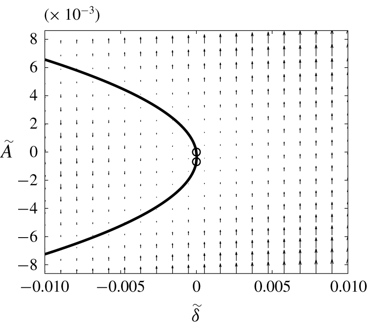
Equation (7.5) describes a well-known saddle-node bifurcation. It has either two fixed points corresponding to equilibrium amplitudes
 $$\begin{eqnarray}A_{e\,1,2}=\pm \sqrt{-\frac{K_{1}}{K_{2}}\unicode[STIX]{x1D6FF}},\end{eqnarray}$$
if the expression under the square root is positive, or none if it is negative. The transition between the two regimes occurs at  $\unicode[STIX]{x1D6FF}=0$, that is, when
 $Re=Re_{\ast \ast }$. The fixed point corresponding to positive (negative) amplitude is stable if
 $K_{1}>0$ (
 $K_{1}<0$).
7.2 Evaluation of bifurcation parameters
While the theoretical procedure described in § 7.1 is rather straightforward, its numerical implementation faces serious challenges. The reason for this is that it relies on the availability of the basic flow and perturbation vectors  $\bar{\boldsymbol{w}}$,
 $\boldsymbol{w}^{\prime }$ and the adjoint eigenvector
 $\boldsymbol{w}^{\dagger }$ computed exactly at the bifurcation point
 $\boldsymbol{P}=\boldsymbol{P}_{\ast \ast }$. The steady axisymmetric solution
 $\bar{\boldsymbol{w}}$ is obtained using Newton-type iterations. However, near the saddle-node bifurcation point, the convergence of such iterations is not guaranteed. In fact, the loss of the iteration convergence was used in Suslov & Cuevas (Reference Suslov, Cuevas, Droniou, Page and Clarke2017), Suslov et al. (Reference Suslov, Pérez-Barrera and Cuevas2017) to indicate the existence of a saddle-node bifurcation in this problem. Therefore, in practice, the above solutions can only be reliably obtained for a parametric set
 $\boldsymbol{P}_{0}$ that is close but not identical to the critical parameters. At
 $\boldsymbol{P}=\boldsymbol{P}_{0}$ the Type 1 and 2 solutions can still be clearly distinguished and the linear amplification rates
 $\unicode[STIX]{x1D70E}(P_{0})$ of the corresponding infinitesimal perturbations are small but non-zero:
 $\unicode[STIX]{x1D70E}(\boldsymbol{P}_{0})=\unicode[STIX]{x1D700}\unicode[STIX]{x1D70E}_{0}$. Then the procedure outlined in § 7.1 results in an additional term on the right-hand side of (7.5),
 $$\begin{eqnarray}\frac{\,\text{d}A}{\,\text{d}t_{1}}=\unicode[STIX]{x1D70E}_{0}A+K_{1}\unicode[STIX]{x1D6FF}+K_{2}A^{2},\end{eqnarray}$$
where now  $\unicode[STIX]{x1D700}^{2}\unicode[STIX]{x1D6FF}=(Re-Re_{0})/Re_{0}=(Fr-Fr_{0})/Fr_{0}$ and
 $Re_{0}$ and
 $Fr_{0}=kRe_{0}$ are the values of the Reynolds and Froude numbers at which the perturbation fields can still be reliably computed, that is
 $Re_{0}\neq Re_{\ast \ast }$. Since a saddle-node bifurcation is structurally stable, for finite values of
 $\unicode[STIX]{x1D6FF}$ the addition of such a term results only in a small quantitative shift of fixed points
 $$\begin{eqnarray}A_{e\,1,2}=\frac{-\unicode[STIX]{x1D70E}_{0}\pm \sqrt{\unicode[STIX]{x1D70E}_{0}^{2}-4K_{1}K_{2}\unicode[STIX]{x1D6FF}}}{2K_{2}}\approx -\frac{\unicode[STIX]{x1D70E}_{0}}{2K_{2}}\pm \sqrt{-\frac{K_{1}}{K_{2}}\unicode[STIX]{x1D6FF}},\end{eqnarray}$$
that disappears as  $Re_{0}\rightarrow Re_{\ast \ast }$ and
 $\unicode[STIX]{x1D70E}(\boldsymbol{P}_{0})\rightarrow 0$.
However, approaching the singularity at  $\boldsymbol{P}_{\ast \ast }$ has a much more detrimental effect on the procedure of § 7.1, that relies on the use of the adjoint eigenvector. While a matrix and its adjoint must have complex conjugate eigenvalues, an attempt to compute eigenvalues of
 ${\mathcal{L}}^{\dagger }$ in the vicinity of
 $\boldsymbol{P}_{\ast \ast }$ using standard numerical linear algebra algorithms (e.g. QR factorisation) results in multiple near-zero eigenvalues, none of which are identical (in the conjugate sense) to the
 $\unicode[STIX]{x1D70E}$ values of
 ${\mathcal{L}}$. Many of these eigenvalues appear to be spurious as they are not present in the spectrum of
 ${\mathcal{L}}$ and depend (unpredictably) on the specifics of the used discretisation. Given that they are clustered densely near 0, identifying the ‘physical’ near-zero value among them becomes virtually impossible. Thus, while one still can reliably compute
 $\bar{\boldsymbol{w}}(P_{0})$ and
 $\boldsymbol{w}^{\prime }(\boldsymbol{P}_{0})$, this is not so for
 $\boldsymbol{w}^{\dagger }(\boldsymbol{P}_{0})$ and one cannot proceed with using the solvability condition (7.6) to determine the values of parameters
 $K_{1,2}$.
To overcome this difficulty we follow an alternative procedure that does not involve the use of an adjoint eigenvector. The idea of this method was first introduced in Crouch & Herbert (Reference Crouch and Herbert1993) and was subsequently refined in Suslov & Paolucci (Reference Suslov and Paolucci1997) and Dey & Suslov (Reference Dey and Suslov2016). The formal algorithmic proof was recently given in Pham & Suslov (Reference Pham and Suslov2018). It has been shown there that, in the vicinity of a bifurcation point, where  $\unicode[STIX]{x1D70E}\neq 0$, the solvability condition (7.6) defining constants in the amplitude equation can be replaced by the orthogonality condition
 $\langle \boldsymbol{w}_{1,2},\boldsymbol{M}\boldsymbol{w}^{\prime }\rangle =0$, where
 $\boldsymbol{M}$ is a weight matrix such that
 $\boldsymbol{M}\boldsymbol{w}^{\prime }\neq \mathbf{0}$. This condition does not require the use of the adjoint eigenvector but, as proven in Suslov & Paolucci (Reference Suslov and Paolucci1997) and Pham & Suslov (Reference Pham and Suslov2018), it produces values identical to those given by (7.6) in the limit of
 $\unicode[STIX]{x1D70E}\rightarrow 0$. Here, we choose
 $\boldsymbol{M}={\mathcal{B}}$, which enforces the orthogonality of the first- and second-order perturbation velocity fields and leads to the following extended systems of equations for
 $\boldsymbol{w}_{1,2}$ and
 $K_{1,2}$:
 $$\begin{eqnarray}\left[\begin{array}{@{}cc@{}}{\mathcal{L}}_{0,0;\boldsymbol{P}_{0}} & -{\mathcal{B}}\boldsymbol{ w}^{\prime }\\[6.0pt] ({\mathcal{B}}\boldsymbol{w}^{\prime })^{H} & 0\end{array}\right]\left[\begin{array}{@{}c@{}}\boldsymbol{w}_{1}\\[6.0pt] K_{1}\end{array}\right]=\left[\begin{array}{@{}c@{}}\boldsymbol{f}_{1}\\[6.0pt] 0\end{array}\right],\quad \left[\begin{array}{@{}cc@{}}{\mathcal{L}}_{2\unicode[STIX]{x1D70E}_{0},0;\boldsymbol{P}_{0}} & -{\mathcal{B}}\boldsymbol{w}^{\prime }\\[6.0pt] ({\mathcal{B}}\boldsymbol{w}^{\prime })^{H} & 0\end{array}\right]\left[\begin{array}{@{}c@{}}\boldsymbol{w}_{2}\\[6.0pt] K_{2}\end{array}\right]=\left[\begin{array}{@{}c@{}}\boldsymbol{f}_{2}\\[6.0pt] 0\end{array}\right].\end{eqnarray}$$
In writing the above we take into account that, in the limit of  $A\rightarrow 0$,
 $$\begin{eqnarray}\frac{\,\text{d}A}{\,\text{d}t_{1}}\sim \unicode[STIX]{x1D70E}_{0}A\Longrightarrow A\sim \exp (\unicode[STIX]{x1D70E}_{0}t_{1})\Longrightarrow A^{2}\sim \exp (2\unicode[STIX]{x1D70E}_{0}t_{1})\Longrightarrow \frac{\,\text{d}A^{2}}{\,\text{d}t_{1}}\sim 2\unicode[STIX]{x1D70E}_{0}A^{2}.\end{eqnarray}$$
Note that  $\unicode[STIX]{x1D70E}_{0}\neq 0$ since
 $\boldsymbol{P}_{0}\neq \boldsymbol{P}_{\ast \ast }$ and the operators
 ${\mathcal{L}}_{0,0;\boldsymbol{P}_{0}}$ and
 ${\mathcal{L}}_{2\unicode[STIX]{x1D70E},0;\boldsymbol{P}_{0}}$ are non-singular. Thus solutions of equations corresponding to the top rows in (7.10) can be obtained for any values of parameters
 $K_{1,2}$. Therefore, an additional condition, such as the one chosen here and added in the bottom rows in (7.10), is needed to make the solution unique. An interested reader is referred to Pham & Suslov (Reference Pham and Suslov2018) for further details and interpretation. In the context of this work, only two practical points are of importance. The first is that, in contrast to (7.4), the (regularised) problem (7.10) can be solved using standard numerical algorithms for non-singular problems for parametric values close but not identical to
 $\boldsymbol{P}_{\ast \ast }$. This way the numerical difficulties associated with the need for ‘inverting’ singular matrices at
 $\boldsymbol{P}_{\ast \ast }$ and computing the adjoint eigenvector are avoided. The second is that, although the choice of the weight matrix
 $\boldsymbol{M}$ (
 $\boldsymbol{M}={\mathcal{B}}$ here) is quite arbitrary, in the limit of
 $(\boldsymbol{P}_{0}\rightarrow \boldsymbol{P}_{\ast \ast },\unicode[STIX]{x1D70E}_{0}\rightarrow 0)$ the solutions
 $\boldsymbol{w}_{1,2}$ and
 $K_{1,2}$ obtained from (7.10) converge to those of (7.4) with (7.6). Therefore, the solution of a singular problem at a bifurcation point can be obtained with a very good accuracy by considering a non-singular problem in its close vicinity.
7.3 Numerical results for the post-bifurcation regime
In this section we demonstrate the application of the procedure described in § 7.2 to the analysis of the flow behaviour in an electrolyte layer of non-dimensional depth  $\unicode[STIX]{x1D716}=0.248$. The largest value of
 $Re_{0}$ for which we could obtain converged steady-state axisymmetric solutions was
 $Re_{0}=1493.88$. The Type 1 and Type 2 solutions could still be distinguished at this parametric point with the corresponding linear disturbance amplification rates being small but non-zero, see the region near the right ‘nose’ in figure 5(a). However, the attempt to compute the corresponding adjoint eigenvectors at this value of
 $Re_{0}$ failed. Therefore, to find the approximate post-bifurcation flow fields we resorted to solving systems (7.10). The numerical values of coefficients entering equation (7.8) are listed in table 4 for Type 1 and 2 solutions (lower and upper branches of the
 $\unicode[STIX]{x1D70E}^{R}$ curves in figure 5(a), respectively).


The coefficients  $K_{1,2}$ have the same sign for both types of flow. Therefore, as follows from (7.9), the two fixed points corresponding to Type 1 and 2 flows exist only for
 $\unicode[STIX]{x1D6FF}\lesssim 0$, that is for
 $Re<Re_{\ast \ast }$. This is consistent with results presented in figures 5 and 9, and the general discussion given in § 5.
The real fixed points (7.9) cease to exist when the expression under the square root becomes negative. Therefore, with a very good accuracy, we can estimate the location of a saddle-node bifurcation as
 $$\begin{eqnarray}Re_{\ast \ast }=Re_{0}(1+\unicode[STIX]{x1D700}^{2}\unicode[STIX]{x1D6FF}_{\ast \ast }),\text{ where }\unicode[STIX]{x1D6FF}_{\ast \ast }=\frac{\unicode[STIX]{x1D70E}_{0}^{2}}{4K_{1}K_{2}}.\end{eqnarray}$$
In section (5) we reported the critical parameter value  $Re_{\ast \ast }\approx 1494$ that was obtained using a cubic spline fit to the data presented in figure 5. Table 4 contains more precise values obtained using (7.11). Despite the fact that the coefficients computed for the Type 1 and 2 solutions are somewhat different, indicating a slight asymmetry at
 $Re_{0}\neq Re_{\ast \ast }$, the two estimated values of
 $Re_{\ast \ast }$ are in excellent agreement with each other, demonstrating the robustness of the procedure detailed in § 7.2.
Saddle-node bifurcation diagram corresponding to parameters listed in table 4 for the Type 2 solution. The circles show the values of the amplitude at  $Re_{0}$.

Meridional velocity (a) and azimuthal vorticity (b) fields for the steady axisymmetric basic flow solution near the saddle-node bifurcation point for  $\unicode[STIX]{x1D716}=0.248$,
 $Ha=5.08\times 10^{-3}$ and
 $Re=Re_{0}=1493.88\approx Re_{\ast \ast }$. The colour coding is the same as in figure 2.

Variation of axisymmetric perturbation velocity (a) and azimuthal vorticity (b) fields near the saddle-node bifurcation point for the same parameter values as in figure 12.

Meridional perturbation velocity (a) and azimuthal vorticity (b) fields corresponding to the azimuthal wavenumber  $m=0$ for the same parameter values as in figure 12.

The saddle-node bifurcation diagram constructed for the Type 2 solution is shown in figure 11 (the diagram for the Type 1 solution is qualitatively similar with the only difference being that the direction of the amplitude flow is reversed). At the computational point  $Re_{0}$, where the bifurcation parameters are computed (
 $\unicode[STIX]{x1D6FF}=0$), the values of the equilibrium amplitude are
 $A_{e}=0$ (unstable fixed point) and
 $\tilde{A}_{e}=-\unicode[STIX]{x1D70E}(\boldsymbol{P}_{0})/K_{2}\approx -6.9\times 10^{-4}$ (stable fixed point). They are shown by circles in the figure. Beyond the bifurcation point
 $\unicode[STIX]{x1D700}^{2}\unicode[STIX]{x1D6FF}_{\ast \ast }\approx 2.7\times 10^{-5}$ the amplitude
 $\tilde{A}$ becomes and remains positive. This information enables us to reconstruct the axisymmetric component of the flow once it becomes unsteady at
 $\unicode[STIX]{x1D6FF}\gtrsim \unicode[STIX]{x1D6FF}_{\ast \ast }$ (
 $Re\gtrsim Re_{\ast \ast }$) using fields computed for
 $Re_{0}<Re_{\ast \ast }$ without an explicit time integration. We discuss the details of such flow fields, depicted in figures 12–15, next.
Figure 12 shows the converged basic flow fields at  $Re=Re_{0}\lesssim Re_{\ast \ast }$. Topologically, they correspond to a toroidal flow with a secondary recirculation seen for lower Reynolds numbers in the top outer corner of a meridional cross-section (see figure 3) completely suppressed. Figure 13 demonstrates that, despite the increase of the electric current driving the flow beyond the bifurcation point (for
 $\unicode[STIX]{x1D6FF}>\unicode[STIX]{x1D6FF}_{\ast \ast }>0$), the primary meridional circulation and circumferential jet are retarded, creating conditions for the reappearance of the secondary corner circulation; see the bottom plot in figure 13. This is followed by the development of a jet structure with a growing (positive, see figure 11) amplitude
 $A$ that opposes the basic circumferential flow in the top outer corner of a meridional cross-section, see figure 14. When the amplitude of such a jet becomes finite, the nonlinear self-interaction of such a perturbation mode results in a further enhancement of the corner jet and, subsequently, in a more energetic collision of the basic flow and perturbation streams near the free surface, see figure 15. This is where the vortices subsequently arise. While experiments reported in Pérez-Barrera et al. (Reference Pérez-Barrera, Pérez-Espinoza, Ortiz, Ramos and Cuevas2015) indicate that such vortices appear to be qualitatively similar in shape to those observed for
 $Re<Re_{\ast \ast }$, they arise over an unsteady axisymmetric flow background and thus are characterised by a temporally varying intensity.
Second-order meridional axisymmetric perturbation velocity (a) and azimuthal vorticity (b) fields for the same parameter values as in figure 12.

8 Further note on the flow evolution at  $Re\lesssim Re_{\ast }$

While the discussion presented so far sheds light on the flow features beyond the saddle-node bifurcation at  $Re>Re_{\ast \ast }$, the question arises as to whether the analysis developed in § 7 can be applied to clarify the flow evolution near
 $Re=Re_{\ast }$, where the Type 2 solution arises abruptly and is immediately destabilised by the appearing vortices. There are two principle differences between the behaviour of flow solutions near
 $Re_{\ast }$ and
 $Re_{\ast \ast }$. The first is that, while at
 $Re_{\ast \ast }$ the Type 1 and 2 solutions merge together in a continuous way before annihilating each other (which is the signature of a saddle-node bifurcation), at
 $Re_{\ast }$, they remain disjoint (in the sense that they have significantly different spatial structures). Therefore, the transition between Type 1 and Type 2 solutions that occurs at
 $Re_{\ast }$ is not a result of a saddle-node bifurcation involving them. The second distinction is that, while for
 $m=0$ the corresponding eigenvalues
 $\unicode[STIX]{x1D70E}\rightarrow 0$ as
 $Re\rightarrow Re_{\ast }$ or
 $Re\rightarrow Re_{\ast \ast }$, the
 $\unicode[STIX]{x1D70E}^{R}$ values corresponding to other wavenumbers remain strictly negative near
 $Re_{\ast \ast }$ but can become positive near
 $Re_{\ast }$. This signifies the presence of non-stationary growing modes for
 $Re\sim Re_{\ast }$, so that the analysis involving only the
 $m=0$ modes presented in § 7 may be insufficient there and needs to be extended to include growing vortex modes. This requires a significant algebraic effort and is left for a separate publication. However, by formally ignoring the growing modes near
 $Re_{\ast }$ and developing an expansion (7.2) of the stationary axisymmetric solution component there, we arrive at equation (7.8) with coefficients listed in the bottom row of table 4. While such a reduced model is incomplete, it still produces several noteworthy results. In particular, given that the perturbation amplitude
 $A$ should vanish at
 $Re_{\ast }$, from equation (7.11) we find a more accurate value of
 $Re_{\ast }\approx 1031.35$ that is impossible to obtain directly due to the deterioration of iteration convergence near the critical point at which the Type 2 solution ceases to exist. The meridional flow fields computed near
 $Re_{\ast }$ are qualitatively similar to those shown in figures 12–15 and thus are not presented here. Yet, in contrast to regimes corresponding to
 $Re>Re_{\ast \ast }$, when
 $Re<Re_{\ast }$, the solution
 $A(t)$ (and its time derivative) of the amplitude equation (7.8) with coefficients listed in the last row of table 4 remains negative. The implication of this fact is that the perturbation fields
 $A\boldsymbol{w}^{\prime }$ and
 $\unicode[STIX]{x1D6FF}\boldsymbol{w}_{1}$ have the opposite direction to that in figures 14 and 13. The qualitative interpretation of this fact is that, when these fields are superposed onto the Type 2 basic flow shown in figure 3, they lead to the intensity reduction of the secondary toroidal structure and eventually to its complete suppression. Therefore, the Type 2 solution abruptly collapses to the Type 1 solution, where the secondary toroidal flow structure leading to the formation of vortices is absent. Having made this qualitative conclusion, we emphasise once again that a detailed analysis of an unsteady behaviour of the flow near
 $Re_{\ast }$ requires considering a nonlinear multi-mode interaction that is not attempted here.
9 Conclusions
We conducted a comprehensive linear stability study of steady axisymmetric solutions for the electrolyte flow occurring in a thin free-surface annular layer of electrolyte driven by the Lorentz force. For small values of the applied radial current that correspond to small flow Reynolds numbers, only one-torus steady flow (Type 1) exists. As the value of the current increases, the two-torus basic flow (Type 2) arises abruptly and vortices near the outer boundary develop on its background. As the current strengthens further, both the number of linearly unstable modes (vortices) and their growth rates change. Eventually the linear amplification rate becomes negative for all azimuthal wavenumbers, which may be interpreted as the stabilisation of an axisymmetric flow. However, this contradicts experimental observations. We found that, in reality, this behaviour indicates the presence of a saddle-node bifurcation, where Type 1 and Type 2 steady axisymmetric solutions ‘collide’ and annihilate each other. Beyond this point, only an unsteady solution can exist. We approximated it using the amplitude expansion approach and showed that, indeed, the amplitude of the perturbed solutions satisfies a canonical equation describing saddle-node bifurcation that, to the best of our knowledge, has not been reported in the literature for other rotating flows in similar geometries.
To pinpoint the physical mechanisms driving the observed instabilities, we also derived the linearised perturbation energy balance equation. It enabled us to conclude that Rayleigh’s inviscid centrifugal instability mechanism aided by radial shear in the boundary layer near the outer cylindrical wall is responsible for vortex formation with electromagnetic effects being negligible. This mechanism appears to be very robust. A very similar instability pattern has been recently observed by Pérez-Barrera et al. (Reference Pérez-Barrera, Ramírez-ZÚñiga, Grespan, Cuevas and del Río2019) in experiments, where the inner cylindrical electrode was replaced with a fully submerged disk electrode eliminating the no-slip velocity condition at the inner vertical boundary. This significantly changes the velocity profile in its vicinity. Nevertheless, the qualitative structure of instability with a vortex system appearing near the outer cylindrical wall persists, once again confirming that centrifugal effects rather than viscous shear lead to the formation of the observed vortices.
Finally, we mention that recently Antar et al. (Reference Antar, Lalti and Habchi2019) have repeated experiments previously described by Pérez-Barrera et al. (Reference Pérez-Barrera, Pérez-Espinoza, Ortiz, Ramos and Cuevas2015) and Suslov et al. (Reference Suslov, Pérez-Barrera and Cuevas2017) after building a similar apparatus. They focussed on observing instabilities that we analysed here. While experimental results described by Antar et al. (Reference Antar, Lalti and Habchi2019) are generally consistent with and complement those reported previously, these authors neglected to correlate their findings with a detailed discussion of non-trivial physical mechanisms driving the considered flows given in Suslov et al. (Reference Suslov, Pérez-Barrera and Cuevas2017) and postulated their own conclusions instead. In particular, among multiple other inconsistencies found in their discussion, they claim that Kelvin–Helmholtz instability is responsible for the observed vortex formation. The current study demonstrates that this is physically not the case.
Acknowledgement
J.McC. acknowledges support through an Australian Government Research Training Program Scholarship.
Declaration of interests
The authors report no conflict of interest.