1. Introduction
Automation allows machines to perform tasks that are previously performed by workers. On the one hand, automation may be a threat to the employment of workers. For example, a recent study by Frey and Osborne (Reference Frey and Osborne2017) examines 702 occupations and finds that almost half of them could be automated within the next two decades. On the other hand, automation reduces the cost of production and frees up resources for more productive activities. Given the rising importance of automation,Footnote 1 we develop a growth model with automation to explore its effects on the macroeconomy.
Specifically, we introduce automation in the form of capital-labor substitution into a Schumpeterian growth model. Then, we apply the model to explore the effects of R&D subsidy versus automation subsidy on innovation, economic growth, and the welfare of different agents in the economy. In our model, an industry uses labor as the factor input before automation occurs. When the industry becomes automated, it then uses capital as the factor input. Innovation in the form of a quality improvement can arrive at an automated or unautomated industry. When an innovation arrives at an automated industry, the industry becomes unautomated and once again uses labor as the factor input. Therefore, the share of automated industries, which is also the degree of capital intensity in the aggregate production function, is endogenously determined by automation and innovation.
In this growth-theoretic framework, we obtain the following results. An increase in R&D subsidy leads to a higher level of innovation and a higher rate of economic growth. However, the increase in skilled labor for innovation crowds out skilled labor for automation and leads to a lower share of automated industries as well as a lower degree of capital intensity in the aggregate production function. This effect is absent in previous studies with exogenous capital intensity in production. Capital intensity affects output and welfare because it determines the returns to scale of capital, which is a reproducible factor that can be accumulated. An increase in automation subsidy has a negative effect on innovation and economic growth but a positive effect on the share of automated industries and capital intensity in production.
We also calibrate the model to aggregate US data and obtain the following quantitative results. Increasing R&D subsidy increases the welfare of high-skill workers but decreases the welfare of low-skill workers and capital owners. Intuitively, high-skill workers engage in innovative activities and benefit from R&D subsidies, which however hurt low-skill workers and capital owners due to the tax burden from increasing subsidies and the lower capital share of income.
Furthermore, increasing automation subsidy increases the welfare of high-skill workers and also capital owners but decreases the welfare of low-skill workers. Intuitively, high-skill workers also engage in automation and benefit from the subsidies, whereas capital owners benefit from the higher capital share of income. However, low-skill workers are worse off due to the tax burden from increasing subsidies and the lower labor share of income. Therefore, whether the government should subsidize automation depends on how it evaluates the welfare gains and losses of different agents in the economy. Simulating transition dynamics, we find that increasing the automation subsidy rate by 5 percentage points leads to a welfare gain equivalent to a permanent increase in consumption of 3.14% for capital owners and 2.35% for high-skill workers as well as a welfare loss of 1.47% for low-skill workers.
This study relates to the literature on innovation and economic growth. Romer (Reference Romer1990) develops the seminal R&D-based growth model in which innovation is driven by the invention of new products. Then, Segerstrom et al. (Reference Segerstrom, Anant and Dinopoulos1990), Grossman and Helpman (Reference Grossman and Helpman1991), and Aghion and Howitt (Reference Aghion and Howitt1992) develop the Schumpeterian quality-ladder model in which innovation is driven by the development of higher-quality products. Many subsequent studies in this literature use variants of the R&D-based growth model to explore the effects of R&D subsidies; see for example, Peretto (Reference Peretto1998), Segerstrom (Reference Segerstrom2000), Zeng and Zhang (Reference Zeng and Zhang2007), Impullitti (Reference Impullitti2010), Chu et al. (Reference Chu, Furukawa and Ji2016), and Chu and Cozzi (Reference Chu and Cozzi2018). These studies do not feature automation, and hence, the degree of capital intensity in the aggregate production function is exogenous or simply zero.
This study also relates to the literature on automation and innovation; see Aghion et al. (Reference Aghion, Jones and Jones2017) for a comprehensive discussion of this literature. An early study by Zeira (Reference Zeira1998) develops a growth model with capital-labor substitution, which forms the basis of automation in subsequent studies. Zeira (Reference Zeira2006) contributes to the literature by introducing endogenous invention of technologies into Zeira (Reference Zeira1998). Peretto and Seater (Reference Peretto and Seater2013) propose a growth model with factor-eliminating technical change in which R&D serves to increase capital intensity in the production process. Our study relates to Peretto and Seater (Reference Peretto and Seater2013) by considering both factor-eliminating technical change (i.e. automation) and factor-augmenting technical change (i.e. innovation) and exploring their relative importance on growth and welfare. Recent studies by Acemoglu and Restrepo (Reference Acemoglu and Restrepo2018) and Hemous and Olson (Reference Hemous and Olsen2022) generalize the model in Zeira (Reference Zeira1998) and introduce directed technological change between automation and variety expansion in order to explore the effects of automation on the labor market and income inequality.Footnote 2 Our study complements these interesting studies by embedding endogenous automation into the Schumpeterian quality-ladder model.Footnote 3 While Acemoglu and Restrepo (Reference Acemoglu and Restrepo2018) assume in their variety-expanding model that when a new unautomated product arrives, a previous automated product becomes obsolete, our Schumpeterian model features an endogenous cycle of innovation and automation on a fixed variety of products. Acemoglu et al. (Reference Acemoglu, Manera and Restrepo2020) examine the optimal combination of income taxes on labor, capital, and automation. They find that it is optimal to levy a tax on automation.Footnote 4 Instead of considering the welfare of a representative household, we consider the different effects of subsidizing R&D versus subsidizing automation on the welfare of high-skill workers, low-skill workers, and capital owners in the economy.
Empirical studies have also examined the effects of automation. For example, Acemoglu and Restrepo (Reference Acemoglu and Restrepo2020) find that automation has a negative effect on employment and wages. Arntz et al. (Reference Arntz, Gregory and Zierahn2017) also find that automation has a negative effect on the number of jobs. Dauth et al. (Reference Dauth, Findeisen, Suedekum and Woessner2017) find that automation has no effect on job losses but a negative effect on the labor-income share. Our theoretical model yields consistent predictions that subsidizing automation would lead to a negative effect on the wage income of production workers, the labor share of income, and the number of industries that hire workers.
The rest of the paper is organized as follows. Section 2 presents the model. Section 3 compares the effects of the two subsidies. Section 4 presents some extensions to the baseline model. The final section concludes.
2. A Schumpeterian growth model with automation
We introduce automation in the form of capital-labor substitution as in Zeira (Reference Zeira1998) into a canonical Schumpeterian growth model. We consider a cycle of automation and innovation. An unautomated industry that currently uses labor as the factor input can become automated and then use capital as the factor input. Innovation in the form of a quality improvement can arrive at an automated or unautomated industry. When an innovation arrives at an automated industry, the industry becomes unautomated and once again uses labor as the factor input until the next automation arrives.Footnote 5 We will derive the equilibrium condition that supports this cycle of automation and innovation.
2.1 Agents
There are three types of agents in the model. Their lifetime utility functions are given by
 \begin{equation} U^{j}=\int _{0}^{\infty }e^{-\rho t}\ln c_{t}^{j}dt\text{,} \end{equation}
where
 $j\in \{k,l,h\}$
.
 $c_{t}^{k}$
is the consumption of a representative capital owner.
 $c_{t}^{l}$
is the consumption of a representative low-skill worker, who engages in the production of goods.
 $c_{t}^{h}$
is the consumption of a representative high-skill worker, who takes on the roles of a scientist in innovation and automation. For simplicity, we assume that they all have the same discount rate
 $\rho >0$
.Footnote 6
Only the capital owner accumulates (tangible and intangible) capital. He/she maximizes utility subject to the following asset-accumulation equation:
 \begin{equation} \dot{a}_{t}+\dot{k}_{t}=r_{t}a_{t}+(R_{t}-\delta )k_{t}-c_{t}^{k}\text{.} \end{equation}
 $a_{t}$
is the real value of assets (i.e. the share of monopolistic firms), and
 $r_{t}$
is the real interest rate.
 $k_{t}$
is physical capital, and
 $R_{t}-\delta$
is the real rental price net of capital depreciation. From standard dynamic optimization, the Euler equation is
 \begin{equation} \frac{\dot{c}_{t}^{k}}{c_{t}^{k}}=r_{t}-\rho \text{.} \end{equation}
Also, the no-arbitrage condition
 $r_{t}=R_{t}-\delta$
holds.
The representative low-skill worker supplies
 $l$
units of low-skill labor. The representative high-skill worker supplies one unit of high-skill labor, which can be allocated between innovation and automation.
 $w_{l,t}$
is the real wage rate of low-skill labor in production, whereas
 $w_{h,t}$
is the real wage rate of high-skill labor in automation and innovation. Workers simply consume their after-tax wage income such that
 $c_{t}^{l}=(1-\tau _{t})w_{l,t}l$
and
 $c_{t}^{h}=(1-\tau _{t})w_{h,t}$
, where
 $\tau _{t}$
is the rate of labor-income tax (or transfer).Footnote 7
2.2 Final good
Competitive firms produce final good
 $y_{t}$
using the following Cobb-Douglas aggregator over a unit continuum of differentiated intermediate goods:Footnote 8
 \begin{equation} y_{t}=\exp \left ( \int _{0}^{1}\ln x_{t}(i)di\right ) \text{.} \end{equation}
 $x_{t}(i)$
denotes intermediate good
 $i\in \lbrack 0,1]$
,Footnote 9 and the conditional demand function for
 $x_{t}(i)$
is
 \begin{equation} x_{t}(i)=\frac{y_{t}}{p_{t}(i)}\text{,} \end{equation}
where
 $p_{t}(i)$
is the price of
 $x_{t}(i)$
.
2.3 Intermediate goods
There is a unit continuum of industries, which are also indexed by
 $i\in \lbrack 0,1]$
, producing differentiated intermediate goods. If an industry is not automated, then the production process uses low-skill labor and the production function is
 \begin{equation} x_{t}(i)=z^{n_{t}(i)}l_{t}(i)\text{,} \end{equation}
where the parameter
 $z>1$
is the step size of each quality improvement,
 $n_{t}(i)$
is the number of quality improvements that have occurred in industry
 $i$
as of time
 $t$
, and
 $l_{t}(i)$
is the amount of low-skill labor employed in industry
 $i$
. Given the productivity level
 $z^{n_{t}(i)}$
, the marginal cost function of the leader in an unautomated industry
 $i$
is
 $w_{l,t}/z^{n_{t}(i)}$
.
The monopolistic price
 $p_{t}(i)$
involves a markup over the marginal cost
 $w_{l,t}/z^{n_{t}(i)}$
. Grossman and Helpman (Reference Grossman and Helpman1991) and Aghion and Howitt (Reference Aghion and Howitt1992) assume that the markup is equal to the quality step size
 $z$
, due to limit pricing between current and previous quality leaders. Here we follow Howitt (Reference Howitt1999) and Dinopoulos and Segerstrom (Reference Dinopoulos and Segerstrom2010) to consider an alternative scenario in which new quality leaders do not engage in limit pricing with previous quality leaders because after the implementation of the newest innovations, previous quality leaders exit the market and need to pay a cost before reentering. Given the Cobb-Douglas aggregator in (4), the unconstrained monopolistic price would be infinite; here, we follow Evans et al. (Reference Evans, Quigley and Zhang2003) to consider price regulation as a policy constraint imposed by the government under which the regulated markup ratio cannot be greater than
 $\mu >1$
such thatFootnote 10
 \begin{equation} p_{t}(i)\leq \mu \frac{w_{l,t}}{z^{n_{t}(i)}}\text{.} \end{equation}
To maximize profit, the industry leader chooses
 $p_{t}(i)=\mu w_{l,t}/z^{n_{t}(i)}$
. In this case, the wage payment in an unautomated industry is
 \begin{equation} w_{l,t}l_{t}(i)=\frac{1}{\mu }p_{t}(i)x_{t}(i)=\frac{1}{\mu }y_{t}\text{,} \end{equation}
and the amount of monopolistic profit in an unautomated industry is
 \begin{equation} \pi _{t}^{l}(i)=p_{t}(i)x_{t}(i)-w_{l,t}l_{t}(i)=\frac{\mu -1}{\mu }y_{t}\text{.} \end{equation}
If an industry is automated, then we follow Zeira (Reference Zeira1998) to assume that the production process uses capital. The production function isFootnote 11
 \begin{equation} x_{t}(i)=\frac{A}{Z_{t}}z^{n_{t}(i)}k_{t}(i)\text{,} \end{equation}
where
 $A>0$
is a parameter that captures an exogenous productivity difference between automated and unautomated industries.
 $Z_{t}$
denotes aggregate technology capturing an erosion effect of new technologies that reduce the adaptability of existing physical capital.Footnote 12 Intuitively, new technologies may not be fully compatible with existing capital, and hence, they reduce the productivity of capital.Footnote 13
Given the productivity level
 $z^{n_{t}(i)}$
, the marginal cost function of the leader in an automated industry
 $i$
is
 $Z_{t}R_{t}/[Az^{n_{t}(i)}]$
. The monopolistic price
 $p_{t}(i)$
also involves a markup
 $\mu$
over the marginal cost
 $Z_{t}R_{t}/[Az^{n_{t}(i)}]$
. Once again, we consider price regulation as a policy constraint under which
 \begin{equation} p_{t}(i)\leq \mu \frac{Z_{t}R_{t}}{Az^{n_{t}(i)}}\text{.} \end{equation}
To maximize profit, the industry leader chooses
 $p_{t}(i)=\mu Z_{t}R_{t}/[Az^{n_{t}(i)}]$
. In this case, the capital rental payment in an automated industry is
 \begin{equation} R_{t}k_{t}(i)=\frac{1}{\mu }p_{t}(i)x_{t}(i)=\frac{1}{\mu }y_{t}\text{,} \end{equation}
and the amount of monopolistic profit in an automated industry is
 \begin{equation} \pi _{t}^{k}(i)=p_{t}(i)x_{t}(i)-R_{t}k_{t}(i)=\frac{\mu -1}{\mu }y_{t}\text{.} \end{equation}
2.4 Automation-innovation cycle
In this section, we derive the equilibrium condition that supports a cycle of automation and innovation. An unautomated industry that currently uses labor as the factor input can become automated and then use capital as the factor input. In order for automation to yield a lower marginal cost of production than an existing innovation, we need the following condition to hold:
 $Z_{t}R_{t}/A<w_{l,t}$
. Then, when an innovation arrives at an automated industry, the industry becomes unautomated and once again uses labor as the factor input until the next automation arrives.Footnote 14 In order for the next innovation to yield a lower marginal cost of production than automation, we need the following condition to hold:
 $w_{l,t}/z<Z_{t}R_{t}/A$
. Combining these two conditions yields
 $w_{l,t}/z<Z_{t}R_{t}/A<w_{l,t}$
. In Lemma 1, we derive the steady-state equilibrium expression for this condition, in which
 $g_{y}\equiv \dot{y}_{t}/y_{t}$
is the steady-state growth rate of output.Footnote 15
Lemma 1 The steady-state equilibrium condition for the automation-innovation cycle is
 \begin{equation*} \frac {1}{z} < \left [ \frac {\mu }{A}\left ( g_{y}+\rho +\delta \right ) \right ] ^{\frac {1}{1-\theta }} < 1\text {.} \end{equation*}
Proof. See the Appendix A.
2.5 R&D and automation
Equations (9) and (13) show that
 $\pi _{t}^{l}(i)=\pi _{t}^{l}$
and
 $\pi _{t}^{k}(i)=\pi _{t}^{k}$
for each type of industries. Therefore, the value of inventions is also the same within each type of industries such that
 $v_{t}^{l}(i)=v_{t}^{l}$
and
 $v_{t}^{k}(i)=v_{t}^{k}$
.Footnote 16 The no-arbitrage condition that determines the value
 $v_{t}^{l}$
of an unautomated invention is
 \begin{equation} r_{t}=\frac{\pi _{t}^{l}+\dot{v}_{t}^{l}-(\alpha _{t}+\lambda _{t})v_{t}^{l}}{v_{t}^{l}}\text{,} \end{equation}
which states that the rate of return on
 $v_{t}^{l}$
is equal to the interest rate. The return on
 $v_{t}^{l}$
is the sum of monopolistic profit
 $\pi _{t}^{l}$
, capital gain
 $\dot{v}_{t}^{l}$
and expected capital loss
 $(\alpha _{t}+\lambda _{t})v_{t}^{l}$
, where
 $\alpha _{t}$
is the arrival rate of automation and
 $\lambda _{t}$
is the arrival rate of innovation.Footnote 17
Similarly, the no-arbitrage condition that determines the value
 $v_{t}^{k}$
of an automation is
 \begin{equation} r_{t}=\frac{\pi _{t}^{k}+\dot{v}_{t}^{k}-\lambda _{t}v_{t}^{k}}{v_{t}^{k}}\text{,} \end{equation}
which states that the rate of return on
 $v_{t}^{k}$
is also equal to the interest rate. The return on
 $v_{t}^{k}$
is the sum of monopolistic profit
 $\pi _{t}^{k}$
, capital gain
 $\dot{v}_{t}^{k}$
and expected capital loss
 $\lambda _{t}v_{t}^{k}$
, where
 $\lambda _{t}$
is the arrival rate of innovation. The condition in Lemma 1 ensures that the previous automation becomes obsolete when the next innovation arrives.
Competitive entrepreneurs recruit high-skill labor
 $h_{r,t}(i)$
to perform innovation across all industries
 $i$
. The arrival rate of innovation in industry
 $i$
is given by
 \begin{equation} \lambda _{t}(i)=\varphi _{t}h_{r,t}(i)\text{,} \end{equation}
where
 $\varphi _{t}\equiv \varphi h_{r,t}^{\epsilon -1}$
in which
 $\varphi >0$
is an innovation productivity parameter. The aggregate arrival rate of innovation is
 $\lambda _{t}=\varphi h_{r,t}^{\epsilon }$
, where
 $h_{r,t}$
denotes aggregate R&D labor.Footnote 18 Here the parameter
 $\epsilon \in (0,1)$
captures an intratemporal duplication externality as in Jones and Williams (Reference Jones and Williams2000) and determines the degree of decreasing returns to scale in R&D at the aggregate level.Footnote 19 In a symmetric equilibrium, the free-entry condition of R&D becomes
 \begin{equation} \lambda _{t}v_{t}^{l}=(1-s)w_{h,t}h_{r,t}\Leftrightarrow \varphi v_{t}^{l}=(1-s)w_{h,t}h_{r,t}^{1-\epsilon }\text{,} \end{equation}
where
 $s<1$
is the R&D subsidy rate.Footnote 20
There are also competitive entrepreneurs who recruit high-skill labor
 $h_{a,t}(i)$
to perform automation in currently unautomated industries. The arrival rate of automation in such industry
 $i$
is given by
 \begin{equation} \alpha _{t}(i)=\phi _{t}h_{a,t}(i)\text{,} \end{equation}
where
 $\phi _{t}\equiv \phi (1-\theta _{t})h_{a,t}^{\epsilon -1}$
in which
 $\phi >0$
is an automation productivity parameter. Once again,
 $\epsilon \in (0,1)$
captures the intratemporal duplication externality and determines the degree of decreasing returns to scale in automation at the aggregate level.Footnote 21 The endogenous variable
 $\theta _{t}\in (0,1)$
is the fraction of industries that are automated at time
 $t$
. In other words,
 $1-\theta _{t}$
captures the following effect: a larger mass of currently unautomated industries that can be automated makes automation easier to complete.Footnote 22 The aggregate arrival rate of automation is
 $\alpha _{t}=\phi h_{a,t}^{\epsilon }$
, where
 $h_{a,t}$
denotes aggregate automation labor, and we have used the condition that
 $h_{a,t}(i)=h_{a,t}/(1-\theta _{t})$
. In a symmetric equilibrium, the free-entry condition of automation becomes
 \begin{equation} \alpha _{t}v_{t}^{k}=(1-\sigma )w_{h,t}h_{a,t}/(1-\theta _{t})\Leftrightarrow \phi (1-\theta _{t})v_{t}^{k}=(1-\sigma )w_{h,t}h_{a,t}^{1-\epsilon }\text{,} \end{equation}
where
 $\sigma <1$
is the automation subsidy rate.Footnote 23
2.6 Government
The government collects tax revenue to finance the subsidies on R&D and automation. The balanced-budget condition is
 \begin{equation} \tau _{t}(w_{l,t}l+w_{h,t})=sw_{h,t}h_{r,t}+\sigma w_{h,t}h_{a,t}\text{.} \end{equation}
2.7 Aggregate economy
Aggregate technology
 $Z_{t}$
is defined asFootnote 24
 \begin{equation} Z_{t}\equiv \exp \left ( \int _{0}^{1}n_{t}(i)di\ln z\right ) =\exp \left ( \int _{0}^{t}\lambda _{\omega }d\omega \ln z\right ) \text{,} \end{equation}
where
 $\int _{0}^{1}n_{t}(i)di\equiv \overline{n}_{t}$
is the aggregate number of innovations that have occurred in the economy and the last equality in (21) uses the law of large numbers. Differentiating the log of
 $Z_{t}$
in (21) with respect to time yields the growth rate of technology given byFootnote 25
 \begin{equation} g_{z,t}\equiv \frac{\dot{Z}_{t}}{Z_{t}}=\lambda _{t}\ln z\text{.} \end{equation}
Substituting (6) and (10) into (4) yields the following familiar Cobb-Douglas aggregate production function:Footnote 26
 \begin{equation} y_{t}=\left ( \frac{Ak_{t}}{\theta _{t}}\right ) ^{\theta _{t}}\left ( \frac{Z_{t}l}{1-\theta _{t}}\right ) ^{1-\theta _{t}}\text{,} \end{equation}
where the share
 $\theta _{t}$
of automated industries also determines the degree of capital intensity in the aggregate production function. The evolution of
 $\theta _{t}$
is determined by
 \begin{equation} \dot{\theta }_{t}=\alpha _{t}(1-\theta _{t})-\lambda _{t}\theta _{t}\text{,} \end{equation}
where
 $\alpha _{t}=\phi h_{a,t}^{\epsilon }$
and
 $\lambda _{t}=\varphi h_{r,t}^{\epsilon }$
are respectively the arrival rates of automation and innovation. Using (2), one can derive the familiar law of motion for capital as follows:Footnote 27
 \begin{equation} \dot{k}_{t}=y_{t}-c_{t}-\delta k_{t}\text{,} \end{equation}
where
 $c_{t}\equiv c_{t}^{k}+c_{t}^{l}+c_{t}^{h}$
. From (8) and (12), the capital and low-skill labor shares of income are
 \begin{equation} \frac{R_{t}k_{t}}{y_{t}}=\frac{\theta _{t}}{\mu }\text{,} \end{equation}
 \begin{equation} \frac{w_{l,t}l}{y_{t}}=\frac{1-\theta _{t}}{\mu }\text{,} \end{equation}
whereas the remaining share
 $(\mu -1)/\mu$
goes to monopolistic profit, which in turn affects high-skill labor income as we will show in Section 3.2.2.
2.8 Decentralized equilibrium
The equilibrium is a time path of allocations
 $\{a_{t},k_{t},c_{t}^{k},c_{t}^{l},c_{t}^{h},y_{t},x_{t}(i),l_{t}(i),k_{t}(i),h_{r,t}(i),h_{a,t}(i)\}$
and a time path of prices
 $\{r_{t},R_{t},w_{l,t},w_{h,t},p_{t}(i),v_{t}^{l}(i),v_{t}^{k}(i)\}$
such that the following conditions hold in each instance:
-
• agents maximize utility taking
 $\{r_{t},R_{t},w_{l,t},w_{h,t}\}$
as given;
-
• competitive final good firms produce
$\{y_{t}\}$
to maximize profit taking
$\{p_{t}(i)\}$
as given; -
• each monopolistic intermediate good firm
$i$
produces
$\{x_{t}(i)\}$
and chooses
$\{l_{t}(i),k_{t}(i),p_{t}(i)\}$
to maximize profit taking
$\{w_{l,t},R_{t}\}$
as given; -
• competitive entrepreneurs choose
$\{h_{r,t}(i),h_{a,t}(i)\}$
to maximize expected profit taking
$\{w_{h,t},v_{t}^{l}(i),v_{t}^{k}(i)\}$
as given; -
• the market-clearing condition for capital holds such that
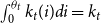
$\int _{0}^{\theta _{t}}k_{t}(i)di=k_{t}$
; -
• the market-clearing condition for low-skill labor holds such that
$\int _{\theta _{t}}^{1}l_{t}(i)di=l$
; -
• the market-clearing condition for high-skill labor holds such that
$\int _{0}^{1}h_{r,t}(i)di+\int _{\theta _{t}}^{1}h_{a,t}(i)di=1$
; -
• the market-clearing condition for final good holds such that
$y_{t}=\dot{k}_{t}+\delta k_{t}+c_{t}^{k}+c_{t}^{l}+c_{t}^{h}$
; -
• the value of inventions is equal to the value of the household’s assets such that
$\int _{0}^{\theta _{t}}v_{t}^{k}(i)di+\int _{\theta _{t}}^{1}v_{t}^{l}(i)di=a_{t}$
; and -
• the government balances the fiscal budget.










3. Growth and welfare effects of R&D and automation
In this section, we consider the growth and welfare effects of R&D and automation subsidies. Section 3.1 explores their effects on economic growth. Section 3.2 explores their effects on the welfare of different groups. Section 3.3 performs a quantitative analysis.
3.1 Economic growth
From (9) and (13), the amount of monopolistic profits in both automated and unautomated industries is
 \begin{equation} \pi _{t}^{l}=\pi _{t}^{k}=\frac{\mu -1}{\mu }y_{t}\text{.} \end{equation}
The balanced-growth values of an innovation and an automation are respectivelyFootnote 28
 \begin{equation} v_{t}^{l}=\frac{\pi _{t}^{l}}{\rho +\alpha +\lambda }=\frac{\pi _{t}^{l}}{\rho +\phi h_{a}^{\epsilon }+\varphi h_{r}^{\epsilon }}\text{,} \end{equation}
 \begin{equation} v_{t}^{k}=\frac{\pi _{t}^{k}}{\rho +\lambda }=\frac{\pi _{t}^{k}}{\rho +\varphi h_{r}^{\epsilon }}\text{.} \end{equation}
Substituting (29) and (30) into the free-entry conditions in (17) and (19) yields
 \begin{equation*} \frac {\varphi (1-\sigma )h_{a}^{1-\epsilon }}{\phi (1-\theta )(1-s)h_{r}^{1-\epsilon }}=\frac {\rho +\phi h_{a}^{\epsilon }+\varphi h_{r}^{\epsilon }}{\rho +\varphi h_{r}^{\epsilon }}\text {,} \end{equation*}
which can be reexpressed as
 \begin{equation} \frac{1-\sigma }{1-s}\left [ \frac{\varphi }{\phi }+\left ( \frac{1-h_{r}}{h_{r}}\right ) ^{\epsilon }\right ] =\left ( \frac{h_{r}}{1-h_{r}}\right ) ^{1-\epsilon }+\left ( \frac{h_{r}}{1-h_{r}}\right ) ^{1-2\epsilon }\frac{\phi }{\varphi +\rho/h_{r}^{\epsilon }}\text{.} \end{equation}
Equation(31) determines the steady-state equilibrium value of R&D labor
 $h_{r}$
. If we assume
 $\epsilon \leq 1/2$
,Footnote 29 then the right-hand side of (31) is increasing in
 $h_{r}$
, whereas the left-hand side is always decreasing in
 $h_{r}$
. Therefore, there exists a unique steady-state equilibrium value of R&D labor
 $h_{r}$
from (31) and automation labor
 $h_{a}=1-h_{r}$
. R&D labor
 $h_{r}(s,\sigma )$
is increasing in R&D subsidy
 $s$
but decreasing in automation subsidy
 $\sigma$
, whereas automation labor
 $h_{a}(s,\sigma )$
is increasing in automation subsidy
 $\sigma$
but decreasing in R&D subsidy
 $s$
.
From (24), the steady-state share of automated industries is
 \begin{equation} \theta (\underset{-}{s},\underset{+}{\sigma })=\frac{\alpha }{\alpha +\lambda }=\frac{\phi h_{a}^{\epsilon }}{\phi h_{a}^{\epsilon }+\varphi h_{r}^{\epsilon }}\text{,} \end{equation}
which is increasing in automation subsidy
 $\sigma$
but decreasing in R&D subsidy
 $s$
. The steady-state equilibrium growth rate of technology is
 \begin{equation} g_{z}(\underset{+}{s},\underset{-}{\sigma })=\lambda \ln z=\varphi h_{r}^{\epsilon }\ln z\text{,} \end{equation}
where
 $h_{r}(s,\sigma )$
is determined in (31) and is increasing in R&D subsidy
 $s$
but decreasing in automation subsidy
 $\sigma$
. Given that
 $y_{t}$
and
 $k_{t}$
grow at the same rate on the balanced-growth path (BGP), the aggregate production function in (23) implies that the steady-state equilibrium growth rate of output
 $y_{t}$
is
 \begin{equation} g_{y}(\underset{+}{s},\underset{-}{\sigma })=g_{z}=\lambda \ln z=\varphi h_{r}^{\epsilon }\ln z\text{,} \end{equation}
where
 $h_{r}(s,\sigma )$
is determined in (31) and is increasing in R&D subsidy
 $s$
but decreasing in automation subsidy
 $\sigma$
. Proposition 1 summarizes these results.
Proposition 1.
An increase in the R&D subsidy rate
 $s$
has a positive effect on the technology growth rate
 $g_{z}$
, a negative effect on the share
 $\theta$
of automated industries, and a positive effect on the output growth rate
 $g_{y}$
. An increase in the automation subsidy rate
 $\sigma$
has a negative effect on the technology growth rate
 $g_{z}$
, a positive effect on the share
 $\theta$
of automated industries, and a negative effect on the output growth rate
 $g_{y}$
.
Proof. See Appendix A.
3.2 Welfare
We now examine the effects of R&D/automation subsidies on the welfare of capital owners, high-skill workers and low-skill workers.Footnote 30 Given that the balanced-growth level of consumption is
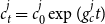 $c_{t}^{j}=c_{0}^{j}\exp (g_{c}^{j}t)$
where
 $g_{c}^{j}$
is the steady-state growth rate of consumption by agent
 $j\in \{k,l,h\}$
, the steady-state level of welfare
 $U^{j}$
can be expressed as
 $U^{j}=\int _{0}^{\infty }e^{-\rho t}(\!\ln c_{0}^{^{j}}+g_{c}^{j}t)dt=(\!\ln c_{0}^{j})/\rho +g_{c}^{j}/\rho ^{2}$
, which in turn can be reexpressed as
 \begin{equation} \rho U^{j}=\ln c_{0}^{j}+\frac{g_{c}^{j}}{\rho }, \end{equation}
for
 $j\in \{k,l,h\}$
. As we will show below,
 $U^{j}$
for
 $j\in \{k,l,h\}$
are all complicated functions; therefore, in Section 3.3, we will simulate the effects of R&D/automation subsidies on the welfare of each group and also the aggregate welfare defined as follows:
 \begin{equation*} U^{a}\equiv U^{k}+U^{l}+U^{h}\text {.} \end{equation*}
3.2.1 Low-skill workers
From
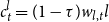 $c_{t}^{l}=(1-\tau )w_{l,t}l$
, the steady-state welfare of low-skill workers is given by
 \begin{equation} \rho U^{l}=\ln\!(1-\tau )+\ln w_{l,0}l+\frac{g_{y}}{\rho }=\ln\!(1-\tau )+\ln \left ( \frac{1-\theta }{\mu }y_{0}\right ) +\frac{g_{y}}{\rho }\text{,} \end{equation}
where the second equality uses (27).
 $U^{l}$
depends on the after-tax wage income of production labor. On the BGP, the wage rate
 $w_{l,t}$
grows at the same rate as output
 $y_{t}$
, which in turn determines the growth rate of low-skill workers’ consumption. Therefore, R&D/automation subsidies affect the welfare of low-skill workers through the tax rate
 $\tau$
, the wage income of production labor and the growth rate of output.
An increase in either subsidy rate leads to a higher tax rate
 $\tau$
. The steady-state share of automated industries is
 $\theta$
is increasing in automation subsidy
 $\sigma$
but decreasing in R&D subsidy
 $s$
as shown in (32), whereas the steady-state output growth rate
 $g_{y}$
is increasing in R&D subsidy
 $s$
but decreasing in automation subsidy
 $\sigma$
as shown in (34). From (23), the initial level of output is given by
 \begin{equation*} y_{0}=\left ( \frac {Ak_{0}}{\theta }\right ) ^{\theta }\left ( \frac {Z_{0}l}{1-\theta }\right ) ^{1-\theta }\text {,} \end{equation*}
which depends on the steady-state share
 $\theta$
of automated industries and the balanced-growth level of capital (derived in Appendix A).
3.2.2 High-skill workers
From
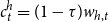 $c_{t}^{h}=(1-\tau )w_{h,t}$
, the steady-state welfare of high-skill workers is given by
 \begin{equation} \rho U^{h}=\ln\!(1-\tau )+\ln w_{h,0}+\frac{g_{y}}{\rho }\text{,} \end{equation}
where the wage rate of high-skill workers can be expressed as
 \begin{equation} w_{h,0}=\frac{\varphi/h_{r}^{1-\epsilon }}{1-s}\frac{\pi _{0}^{l}}{\rho +\phi h_{a}^{\epsilon }+\varphi h_{r}^{\epsilon }}=\frac{\phi (1-\theta )/h_{a}^{1-\epsilon }}{1-\sigma }\frac{\pi _{0}^{k}}{\rho +\varphi h_{r}^{\epsilon }}\text{,} \end{equation}
which uses (17), (19), (29), and (30). Therefore, R&D/automation subsidies affect the welfare of high-skill workers through the tax rate
 $\tau$
, the wage income of research/automation labor, and the growth rate of output.
As before, the tax rate
 $\tau$
is increasing in either subsidy rate, whereas the steady-state output growth rate
 $g_{y}$
is increasing in R&D subsidy
 $s$
but decreasing in automation subsidy
 $\sigma$
as shown in (34). The wage rate of high-skill workers is a complicated function as it depends on several terms, including monopolistic profit which in turn is also determined by the level of output as shown in (28).
3.2.3 Capital owners
The welfare of capital owners can be expressed as
 \begin{equation} \rho U^{k}=\ln c_{0}^{k}+\frac{g_{y}}{\rho }\text{,} \end{equation}
where the initial level of their consumption is given by
 \begin{equation} c_{0}^{k}=\rho (a_{0}+k_{0})\text{,} \end{equation}
which is obtained by imposing balanced growth on (2). Therefore, R&D/automation subsidies affect the welfare of capital owners through the value of intangible/tangible capital and the growth rate of output.
As before, the steady-state output growth rate
 $g_{y}$
is increasing in R&D subsidy
 $s$
but decreasing in automation subsidy
 $\sigma$
as shown in (34). The value of tangible capital
 \begin{equation*} k_{0}=\frac {\theta }{\mu R}y_{0}=\frac {\theta }{\mu\!\left( g_{y}+\rho +\delta \right ) }y_{0}, \end{equation*}
and also the value of intangible capital
 $a_{0}=\theta v_{0}^{k}+(1-\theta )v_{0}^{l}$
are determined by the level of output as shown in (28)–(30).
3.3 Quantitative analysis
In this section, we calibrate the model to aggregate US data in order to perform a quantitative analysis on the growth and welfare effects of the two subsidies. The model features the following set of parameters
 $\{\rho,\delta,\mu,z,\varphi,\phi,\epsilon,s,\sigma,A\}$
.Footnote 31 We choose a conventional value of 0.05 for the discount rate
 $\rho$
. As for the capital depreciation rate
 $\delta$
, we calibrate its value using an investment-capital ratio of 0.0765 in the US. We use the estimate in Laitner and Stolyarov (Reference Laitner and Stolyarov2004) to consider a value of 1.10 for the markup ratio
 $\mu$
. We calibrate the quality step size
 $z$
using a long-run technology growth rate of 0.0125 in the US. We calibrate the R&D productivity parameter
 $\varphi$
using an innovation arrival rate of one-third as in Acemoglu and Akcigit (Reference Acemoglu and Akcigit2012). We calibrate the automation productivity parameter
 $\phi$
using a labor-income share of 0.60 in the US. As for the intratemporal externality parameter
 $\epsilon$
, we follow Jones and Williams (Reference Jones and Williams2000) to set
 $\epsilon$
to 0.5.Footnote 32 Given that the US currently does not apply different rates of subsidies to innovation and automation, we consider a natural benchmark of symmetric subsidies
 $s=\sigma$
.Footnote 33 Then, we follow Impullitti (Reference Impullitti2010) to set the rate of subsidies in the US to 0.188. Finally, the condition for the automation-innovation cycle in Lemma 1 pins down a narrow range of
 $A$
from 0.139 to 0.143 for the values of
 $\{s,\sigma \}$
that we consider, and we pick an intermediate value within this range. Table 1 summarizes the calibrated parameter values.
Calibration

a: Effect of
 $s$
on
 ${g}_{z}$
; b: Effect of
 $s$
on
 $\theta$
; c: Effect of
 $s$
on
 ${g}_{y}$
; d: Effect of
 $s$
on steady-state
 ${U}^{k}$
; e: Effect of
 $s$
on steady-state
 ${U}^{h}$
; f: Effect of
 $s$
on steady-state
 ${U}^{l}$
; and g: Effect of
 $s$
on steady-state
 ${U}^{a}$
.

a: Effect of
 $\sigma$
on
 ${g}_{z}$
; b: Effect of
 $\sigma$
on
 $\theta$
; c: Effect of
 $\sigma$
on
 ${g}_{y}$
; d: Effect of
 $\sigma$
on steady-state
 ${U}^{k}$
; e: Effect of
 $\sigma$
on steady-state
 ${U}^{h}$
; f: Effect of
 $\sigma$
on steady-state
 ${U}^{l}$
; and g: Effect of
 $\sigma$
on steady-state
 ${U}^{a}$
.

In the rest of this section, we simulate the separate effects of R&D subsidy
 $s$
and automation subsidy
 $\sigma$
on the technology growth rate
 $g_{z}$
, the share
 $\theta$
of automated industries, the output growth rate
 $g_{y}$
, and the steady-state welfare
 $U^{j}$
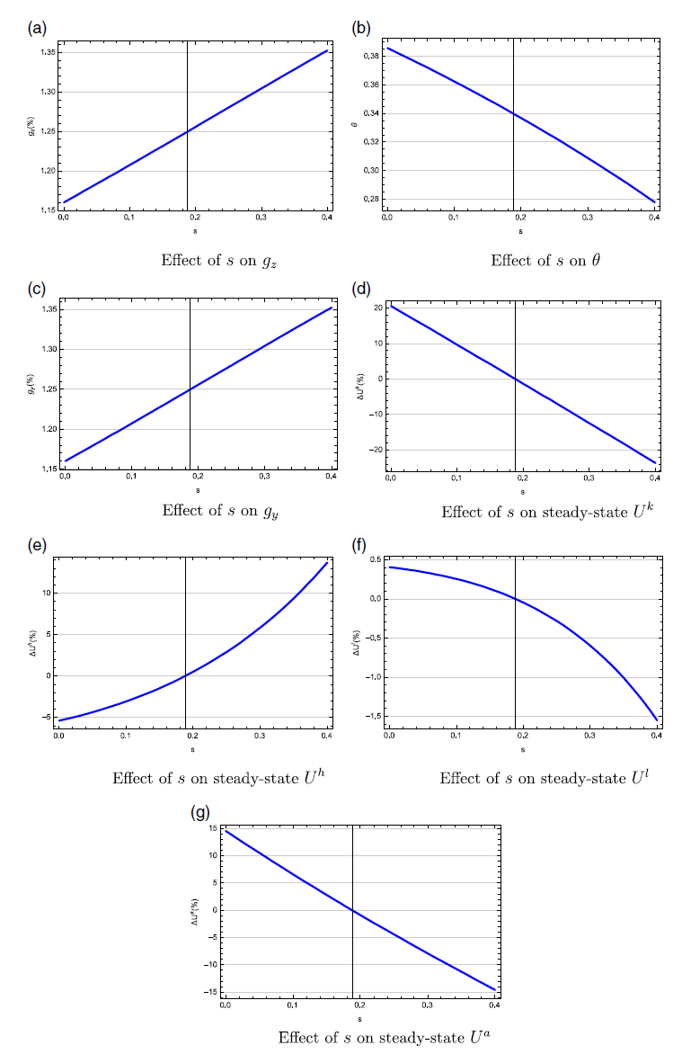
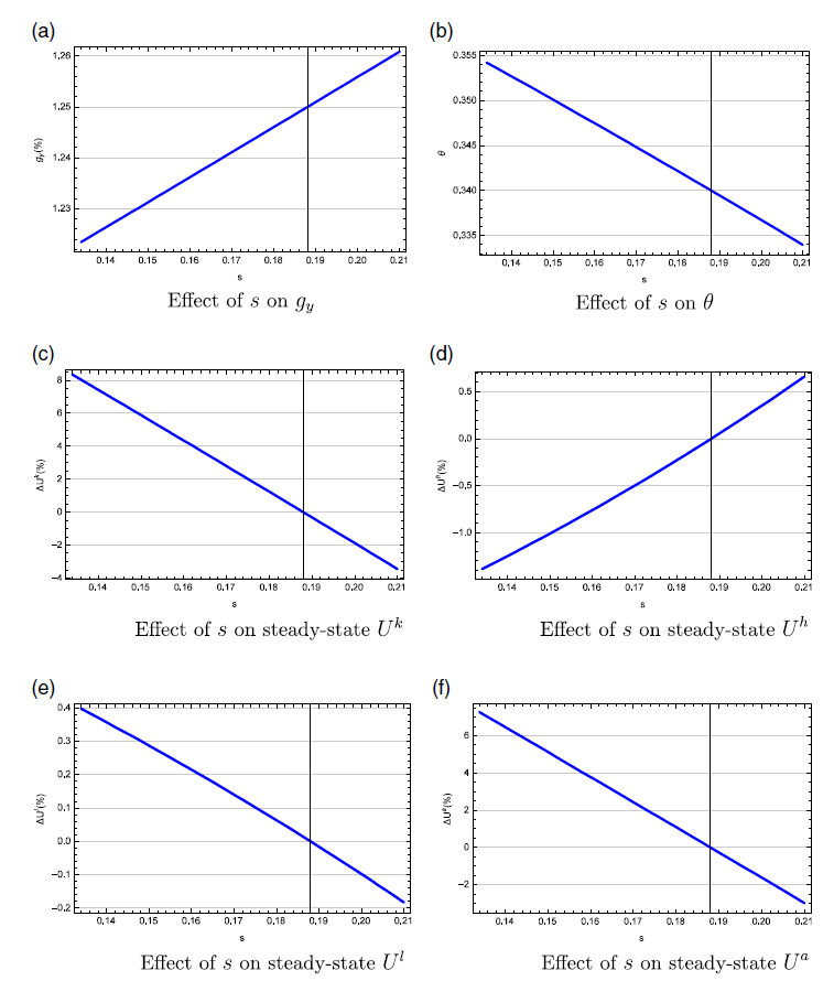
for the three types of agents.Footnote 34 Figure 1 simulates the effects of R&D subsidy
 $s$
. Figure 1a shows that R&D subsidy
 $s$
has a positive effect on the technology growth rate. For example, increasing R&D subsidy
 $s$
from 0.188 to 0.238 raises the technology growth rate from 0.0125 to 0.0127. Figure 1b shows that R&D subsidy
 $s$
has a negative effect on the share of automated industries. Increasing
 $s$
from 0.188 to 0.238 reduces
 $\theta$
from 0.340 to 0.326. Figure 1c shows that R&D subsidy
 $s$
has a positive effect on the growth rate of output. Increasing
 $s$
from 0.188 to 0.238 raises the growth rate of output from 0.0125 to 0.0127. Figure 1d–f shows that R&D subsidy
 $s$
increases the welfare of high-skill workers but decreases the welfare of low-skill workers and capital owners. Increasing
 $s$
from 0.188 to 0.238 leads to a welfare gain equivalent to a permanent increase in consumption of about 2% for high-skill workers as well as a welfare loss of 6% for capital owners and a welfare loss of 0.2% for low-skill workers.Footnote 35 Although all three groups of agents benefit from a higher growth rate
 $g_{y}$
, they experience different welfare effects for the following reasons. High-skill workers engage in R&D and benefit from the subsidies despite the higher tax burden, whereas low-skill workers are hurt by the higher tax burden despite the higher share of production wage income and capital owners are worse off due to the lower capital share of income and the lower capital value.Footnote 36 Figure 1g shows that the overall effect of R&D subsidy
 $s$
on aggregate welfare
 $U^{a}\equiv U^{k}+U^{l}+U^{h}$
is negative. Specifically, increasing
 $s$
from 0.188 to 0.238 leads to an aggregate welfare loss of 4%. This result shows that the welfare loss from capital owners and low-skill workers dominate the welfare gain from high-skill workers when the government increases R&D subsidy.
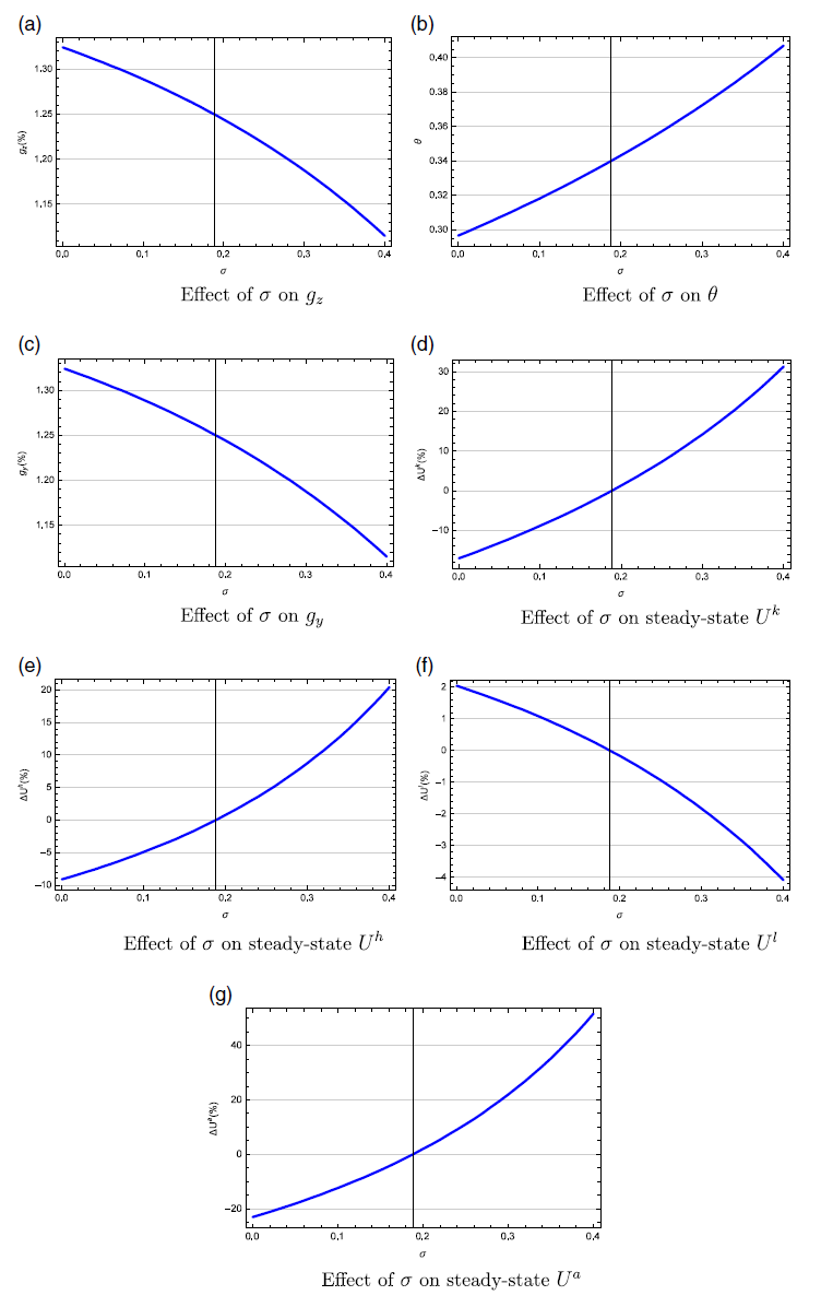
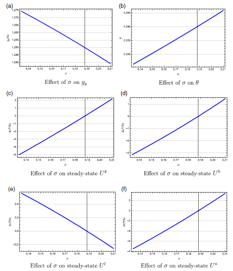
Figure 2 simulates the effects of automation subsidy
 $\sigma$
. Figure 2a shows that automation subsidy
 $\sigma$
has a negative effect on the technology growth rate. For example, increasing automation subsidy
 $\sigma$
from 0.188 to 0.238 reduces the technology growth rate from 0.0125 to 0.0122. Figure 2b shows that automation subsidy
 $\sigma$
has a positive effect on the share of automated industries. Increasing
 $\sigma$
from 0.188 to 0.238 raises
 $\theta$
from 0.340 to 0.354. Figure 2c shows that automation subsidy
 $\sigma$
has a negative effect on the growth rate of output. Increasing
 $\sigma$
from 0.188 to 0.238 reduces the growth rate of output from 0.0125 to 0.0122. Figure 2d–f shows that automation subsidy
 $\sigma$
increases the welfare of high-skill workers and capital owners but decreases the welfare of low-skill workers. Increasing
 $\sigma$
from 0.188 to 0.238 leads to a welfare gain equivalent to a permanent increase in consumption of about 6% for capital owners and 3% for high-skill workers as well as a welfare loss of 0.7% for low-skill workers. In this case, although all three groups of agents are hurt by a lower growth rate
 $g_{y}$
, they experience different welfare effects for the following reasons. High-skill workers engage in automation and benefit from the subsidies despite the higher tax burden, whereas capital owners benefit from the higher capital share of income and the higher capital value; however, low-skill workers are hurt by the higher tax burden and the lower share of production wage income.Footnote 37 Figure 2g shows that the overall effect of automation subsidy
 $\sigma$
on aggregate welfare
 $U^{a}\equiv U^{k}+U^{l}+U^{h}$
is positive and increasing
 $\sigma$
from 0.188 to 0.238 leads to an aggregate welfare gain of 9%. This result shows that the welfare gain from capital owners and high-skill workers dominate the welfare loss from low-skill workers when the government increases automation subsidy.
a: Dynamic effect of
 $\sigma$
on
 ${g}_{z}$
; b: Dynamic effect of
 $\sigma$
on
 $\theta$
; c: Dynamic effect of
 $\sigma$
on
 ${g}_{y}$
; d: Dynamic effect of
 $\sigma$
on
 ${c}^{k}$
; e: Dynamic effect of
 $\sigma$
on
 ${c}^{h}$
; and f: Dynamic effect of
 $\sigma$
on
 ${c}^{l}$
.

3.3.1 Transition dynamics
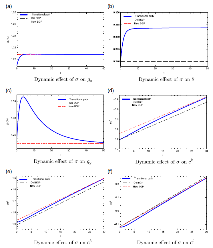
We use the relaxation algorithm in Trimborn et al. (Reference Trimborn, Koch and Steger2008) to simulate the transitional dynamic effects of raising automation subsidy
 $\sigma$
from 0.188 to 0.238.Footnote 38 Figure 3a shows that an increase in automation subsidy leads to a lower technology growth rate
 $g_{z,t}$
. The initial drop in
 $g_{z,t}$
is larger than the decrease in the long run. As shown in Figure 3b, capital intensity
 $\theta _{t}$
increases towards a higher level that requires a large amount of automation labor
 $h_{a,t}$
, which crowds out R&D labor
 $h_{r,t}$
. Figure 3c shows that despite the fall in technology growth
 $g_{z,t}$
, the output growth rate
 $g_{y,t}$
increases after one year before gradually falling towards the new steady state, which is below the initial steady state. The drastic initial increase in output growth
 $g_{y,t}$
is due to the high initial growth in capital intensity
 $\theta _{t}$
.
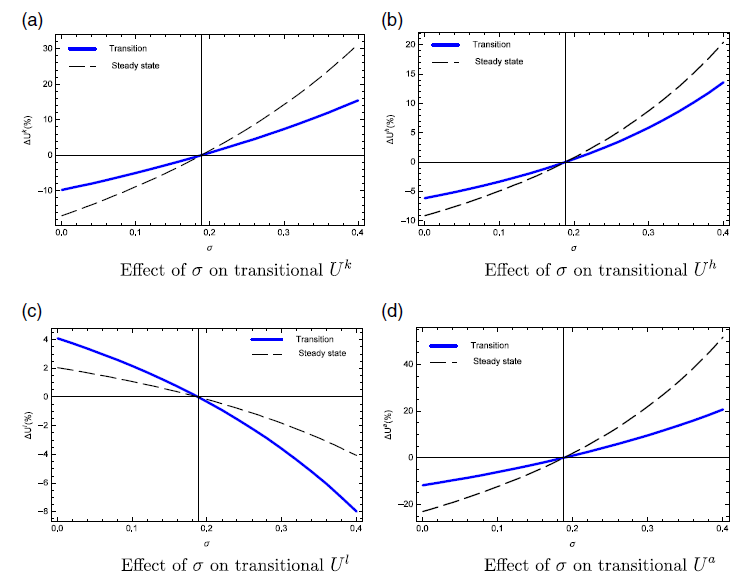
Figure 3d and e show that the (log) level of consumption of capital owners and high-skill workers gradually converges to a higher BGP, which however has a lower growth rate than the initial BGP. Given that the transitional path of consumption is below the new BGP, the transitional welfare gains are likely to be smaller than the steady-state welfare gains computed in the previous section. Figure 3f shows that the level of consumption of low-skill workers falls below the new BGP and gradually converges to it from below. Therefore, the transitional welfare loss on low-skill workers is likely to be larger than the steady-state welfare loss in the previous section. Comparing the new transitional path of consumption and its initial BGP, we compute a welfare gain equivalent to a permanent increase in consumption of 3.14% for capital owners and 2.35% for high-skill workers as well as a welfare loss of 1.47% for low-skill workers. Figure 4a and b show that the transitional welfare effects of automation subsidy
 $\sigma$
on capital owners and high-skill workers are about one-half to two-thirds of the steady-state welfare effects of
 $\sigma$
in Figure 2d–e, whereas Figure 4c shows that the transitional welfare effects of automation subsidy
 $\sigma$
on low-skill workers are about twice the steady-state welfare effects in Figure 2f. Therefore, focusing on the steady state may overstate the welfare effects on some groups but understate the welfare effects on others. Finally, Figure 4d shows that the transitional welfare effects of automation subsidy
 $\sigma$
on aggregate welfare are about one-half of the steady-state welfare effects of
 $\sigma$
in Figure 2g.
a: Effect of
 $\sigma$
on transitional
 ${U}^{k}$
; b: Effect of
 $\sigma$
on transitional
 ${U}^{h}$
; c: Effect of
 $\sigma$
on transitional
 ${U}^{l}$
; and d: Effect of
 $\sigma$
on transitional
 ${U}^{a}$
.

4. Extensions
In this section, we consider a number of extensions to our analysis. Section 4.1 considers a tax on capital income. Section 4.2 considers an alternative specification in which automation also drives economic growth.
4.1 Capital income tax
Suppose we now consider a tax on capital income. Then, the asset-accumulation equation in (3) is modified as
 \begin{equation} \dot{a}_{t}+\dot{k}_{t}=(1-\tau _{t})[r_{t}a_{t}+(R_{t}-\delta )k_{t}]-c_{t}^{k}\text{.} \end{equation}
The consumption path of capital owners in (3) becomes
 \begin{equation} \frac{\dot{c}_{t}^{k}}{c_{t}^{k}}=(1-\tau _{t})r_{t}-\rho \text{,} \end{equation}
where the no-arbitrage condition
 $r_{t}=R_{t}-\delta$
continues to hold. In this case, the government’s balanced-budget condition in (20) is modified as
 \begin{equation} \tau _{t}r_{t}(a_{t}+k_{t})=sw_{h,t}h_{r,t}+\sigma w_{h,t}h_{a,t}\text{.} \end{equation}
The rest of the model remains the same as before. In this case, capital income tax (which finances the two subsidies) gives rise to a distortionary effect on the economy through the interest rate
 $r=(\rho +g_{y})/(1-\tau )$
. This distortionary effect complicates the conditions that determine the equilibrium allocation of high-skill labor; see Appendix D for the derivations.
In the rest of this section, we simulate the growth and welfare effects of R&D/automation subsidies in the presence of this distortionary effect of capital income tax. We recalibrate the model to aggregate data of the US economy to provide a numerical analysis on the growth and welfare effects of the two subsidies. Table 2 summarizes the calibrated parameter values.
Calibration (capital income tax)

Figure 5 simulates the effects of R&D subsidy
 $s$
. Figure 5a–b show that R&D subsidy
 $s$
has a positive effect on the growth rate of output and a negative effect on the share of automated industries. Figure 5c–e show that R&D subsidy
 $s$
increases the welfare of high-skill workers but decreases the welfare of low-skill workers and capital owners. Figure 5f shows that the overall effect of R&D subsidy
 $s$
on aggregate welfare is negative. In summary, the effects of R&D subsidy
 $s$
still follow the same patterns when we consider a tax on capital income.
a: Effect of
 $s$
on
 ${g}_{y}$
; b: Effect of
 $s$
on
 $\theta$
; c: Effect of
 $s$
on steady-state
 ${U}_{k}$
; d: Effect of
 $s$
on steady-state
 ${U}^{h}$
; e: Effect of
 $s$
on steady-state
 ${U}^{l}$
; and f: Effect of
 $s$
on steady-state
 ${U}^{a}$
.

Figure 6 simulates the effects of automation subsidy
 $\sigma$
. Figure 6a–b show that automation subsidy
 $\sigma$
has a negative effect on the growth rate of output and a positive effect on the share of automated industries. Figure 6c–e show that automation subsidy
 $\sigma$
increases the welfare of high-skill workers and capital owners but decreases the welfare of low-skill workers. Figure 6f shows that the overall effect of automation subsidy
 $\sigma$
on aggregate welfare is positive. In summary, the effects of automation subsidy
 $\sigma$
also follow the same patterns when we consider a tax on capital income.
a: Effect of
 $\sigma$
on
 ${g}_{y}$
; b: Effect of
 $\sigma$
on
 $\theta$
; c: Effect of
 $\sigma$
on steady-state
 ${U}_{k}$
; d: Effect of
 $\sigma$
on steady-state
 ${U}^{h}$
; e: Effect of
 $\sigma$
on steady-state
 ${U}^{l}$
; and f: Effect of
 $\sigma$
on steady-state
 ${U}^{a}$
.

4.2 Automation-driven economic growth
We now consider a more general specification for the unautomated production function in (6):
 \begin{equation} x_{t}(i)=\frac{A}{Z_{t}^{\xi }}z^{n_{t}(i)}k_{t}(i)\text{,} \end{equation}
where
 $\xi \in \lbrack 0,1)$
. Then, it can be shown that the aggregate production function in (23) becomes
 \begin{equation} y_{t}=Z_{t}^{1-\xi \theta _{t}}\left ( \frac{Ak_{t}}{\theta _{t}}\right ) ^{\theta _{t}}\left ( \frac{l}{1-\theta _{t}}\right ) ^{1-\theta _{t}}\text{.} \end{equation}
The rest of the model remains the same as in the baseline model in Section 2. Given that
 $y_{t}$
and
 $k_{t}$
grow at the same rate on the BGP, the aggregate production in (45) implies that the steady-state equilibrium growth rate of output
 $y_{t}$
is
 \begin{equation} g_{y}=\left ( \frac{1-\xi \theta }{1-\theta }\right ) g_{z}=\left [ \phi (1-\xi )\left ( 1-h_{r}\right ) ^{\epsilon }+\varphi h_{r}^{\epsilon }\right ] \ln z\text{,} \end{equation}
where the second equality of (46) makes use of (32), (33) and automation labor
 $h_{a}=1-h_{r}$
. In Appendix E, we show that automation subsidy has an additional positive effect on economic growth and gives rise to an overall inverted-U effect on economic growth whenever
 $\xi \in \lbrack 0,1)$
.Footnote 39
5. Conclusion
In this study, we have developed a simple Schumpeterian growth model with automation. Our model features innovation in the form of quality improvement and also automation in the form of capital-labor substitution. Innovation gives rise to technological progress, whereas automation increases the returns to scale of capital in production. R&D subsidy increases innovation but crowds out automation, whereas automation subsidy has the opposite effects. As a result, increasing R&D subsidy has a positive effect on innovation and growth but a negative effect on capital intensity in aggregate production. In contrast, increasing automation subsidy has a negative effect on innovation and growth but a positive effect on capital intensity in aggregate production. Our quantitative analysis shows that increasing R&D subsidy improves the welfare of high-skill workers but hurts the welfare of low-skill workers and capital owners, whereas increasing automation subsidy improves the welfare of high-skill workers and capital owners but hurts the welfare of low-skill workers. In other words, subsidizing automation has different welfare implications on different groups in the economy. Therefore, whether the government should subsidize innovation or automation depends on how it evaluates the welfare gains and losses of different agents in the economy.
To maintain the tractability of the model, we have made a number of simplifying assumptions. Here, we discuss these assumptions and potential extensions for future research. First of all, we have assumed a stylized automation-innovation cycle in which an automation applies only to the current generation of innovation and the next innovation must be produced by labor until it becomes automated. One can generalize this stylized setting by considering the case in which an automation applies to
 $G$
generations of innovation. Here, we consider the special case in which
 $G=1$
, whereas future studies can consider other more interesting cases. Furthermore, we have considered the case in which automation applies to only production but not innovation. One can also consider the case in which both the production and innovation processes can be automated. Finally, we have considered a simple production process with a unitary elasticity of substitution between intermediate goods in which the production of an unautomated good uses only low-skill labor and the production of an automated good uses only capital. One can extend this setting to allow for a non-unitary elasticity of substitution between capital and labor. One can also introduce high-skill labor to the production process and allow for a non-unitary elasticity of substitution between high-skill and low-skill workers in production.Footnote 40 This setting would also allow for an endogenous allocation of high-skill labor between production, automation, and innovation, which generalizes a restriction of our model in which an exogenous supply of high-skill labor is allocated between automation and innovation only.
A. Appendix A: Proofs
Proof of Lemma 1. Using the no-arbitrage condition
 $r=R-\delta$
and the Euler equation
 $r=g_{y}+\rho$
, we can reexpress the equilibrium condition that supports a cycle of automation and innovation as
 \begin{equation} \frac{1}{z} < \frac{Z}{A}\left ( \frac{g_{y}+\rho +\delta }{w_{l}}\right ) < 1\text{.} \end{equation}
We substitute production labor income
 $w_{l}l=\left ( 1-\theta \right ) y/\mu$
and the aggregate production function
 $y=\left ( Ak/\theta \right ) ^{\theta }\left [ Zl/\left ( 1-\theta \right ) \right ] ^{1-\theta }$
into (A.1) to derive
 \begin{equation} \frac{1}{z} < \left ( \frac{1}{A}\right ) ^{\frac{1}{1-\theta }}\left ( \frac{\theta y}{k}\right ) ^{\frac{\theta }{1-\theta }}\left [ \mu\!\left( g_{y}+\rho +\delta \right ) \right ] < 1\text{.} \end{equation}
From capital income
 $Rk=\theta y/\mu$
, the steady-state capital-output ratio is given by
 \begin{equation} \frac{k}{y}=\frac{\theta }{\mu R}=\frac{\theta }{\mu\!\left( r+\delta \right ) }=\frac{\theta }{\mu\!\left( g_{y}+\rho +\delta \right ) }\text{.} \end{equation}
Substituting (A.3) into (A.2) yields the steady-state equilibrium condition for the automation-innovation cycle.
Proof of Proposition 1. We first establish the following sufficient parameter condition for the uniqueness of the equilibrium:
 \begin{equation} \epsilon < \frac{\phi +\rho }{2\phi +\rho }\in (1/2,1)\text{.} \end{equation}
The left-hand side of (31) is decreasing in
 $h_{r}$
, whereas the derivative of the right-hand side of (31) is given by
 \begin{equation} \frac{d}{dh_{r}}RHS=\frac{1}{\left ( 1-h_{r}\right ) ^{2}}\left ( \frac{1-h_{r}}{h_{r}}\right ) ^{\epsilon }\underset{\equiv \Phi }{\underbrace{\left [ \frac{\epsilon \rho \phi\!\left ( 1-h_{r}\right ) ^{1+\epsilon }}{\left ( \varphi h_{r}^{\epsilon }+\rho \right ) ^{2}}+\left ( 1-\epsilon \right ) -\left ( 2\epsilon -1\right ) \frac{\phi\!\left ( 1-h_{r}\right ) ^{\epsilon }}{\varphi h_{r}^{\epsilon }+\rho }\right ] }}\text{.} \end{equation}
Equation (A.5) shows that when
 $\epsilon <1/2$
, right-hand side of (31) is monotonically increasing in
 $h_{r}$
. As for
 $\epsilon >1/2$
, we consider the following lower bound of
 $\Phi$
:
 \begin{equation} \Phi > \left ( 1-\epsilon \right ) -\left ( 2\epsilon -1\right ) \frac{\phi\!\left ( 1-h_{r}\right ) ^{\epsilon }}{\varphi h_{r}^{\epsilon }+\rho } > \left ( 1-\epsilon \right ) -\frac{\phi\!\left ( 2\epsilon -1\right ) }{\rho }\text{.} \end{equation}
Equation (A.6) shows that
 $\epsilon <\left ( \phi +\rho \right )/\left ( 2\phi +\rho \right )$
in (A.1) is a sufficient condition for
 $\Phi >0$
; in this case, right-hand side of (31) is monotonically increasing in
 $h_{r}$
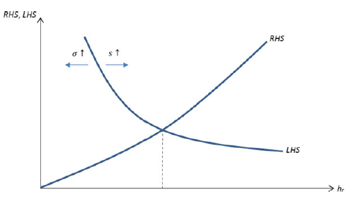
. Therefore, we have established that the equilibrium
 $h_{r}$
is uniquely determined by (31) as shown in Figure 7.
Equilibrium uniqueness.

Left-hand side of (31) being increasing in
 $s$
(decreasing in
 $\sigma$
) implies that
 $h_{r}$
is monotonically increasing from
 $0$
to
 $1$
as
 $s<1\ $
increases on its domain (decreasing from
 $1$
to
 $0$
as
 $\sigma <1$
increases on its domain).Footnote 41 For the effects of
 $\{s,\sigma \}$
on
 $\theta$
, we use (32) to derive that
 $\theta$
is increasing in
 $\sigma$
but decreasing in
 $s$
. As for the effects of
 $\{s,\sigma \}$
on
 $\left \{ g_{z},g_{y}\right \}$
, we use (33) and (34) to establish that both
 $g_{z}$
and
 $g_{y}$
are increasing in
 $s$
but decreasing in
 $\sigma$
.
Balanced-growth level of capital. Using (A.3) and (23), one can derive the balanced-growth level of capital as
 \begin{equation} k_{0}=\left [ \frac{A}{\mu\!\left(g_{y}+\rho +\delta \right ) }\right ] ^{1/(1-\theta )}\frac{\theta }{1-\theta }\frac{lZ_{0}}{A}\text{,} \end{equation}
where the initial level of aggregate technology
 $Z_{0}$
is exogenous.
B. Appendix B: Dynamic equations
This appendix describes the dynamics of the economy. Using (23) and (26), we obtain
 \begin{equation} r_{t}=R_{t}-\delta =\frac{\theta _{t}y_{t}}{\mu k_{t}}-\delta =\frac{A^{\theta _{t}}Z_{t}^{1-\theta _{t}}}{\mu }\left ( \frac{\text{ }\theta _{t}}{1-\theta _{t}}\frac{l}{k_{t}}\right ) ^{1-\theta _{t}}-\delta \text{.} \end{equation}
Based on
 $c_{t}^{l}=(1-\tau _{t})w_{l,t}l$
and
 $c_{t}^{h}=(1-\tau _{t})w_{h,t}$
, we make use of (17), (19), (20) and (27) to obtain
 \begin{equation} \frac{c_{t}^{l}}{k_{t}}+\frac{c_{t}^{h}}{k_{t}}=\frac{(1-\tau _{t})\left ( w_{l,t}l+w_{h,t}\right ) }{k_{t}}=\left ( \frac{1-\theta _{t}}{\mu }\right ) \frac{y_{t}}{k_{t}}+\frac{\lambda _{t}v_{t}^{l}}{k_{t}}+\frac{\alpha _{t}\left ( 1-\theta _{t}\right)\!v_{t}^{k}}{k_{t}}\text{.} \end{equation}
Substituting (B.1) into (3) yields the growth rate of consumption as
 \begin{equation} \frac{\dot{c}_{t}^{k}}{c_{t}^{k}}=\frac{A^{\theta _{t}}Z_{t}^{1-\theta _{t}}}{\mu }\left ( \frac{\text{ }\theta _{t}}{1-\theta _{t}}\frac{l}{k_{t}}\right ) ^{1-\theta _{t}}-\delta -\rho \text{.} \end{equation}
Using (9), (13), (23), (B.1),
 $\lambda _{t}=\varphi h_{r,t}^{\epsilon }$
and
 $\alpha _{t}=\phi h_{a,t}^{\epsilon }$
, we reexpress (14) and (15) as
 \begin{equation} \frac{\dot{v}_{t}^{l}}{v_{t}^{l}}=\frac{A^{\theta _{t}}Z_{t}^{1-\theta _{t}}}{\mu }\left ( \frac{\text{ }\theta _{t}}{1-\theta _{t}}\frac{l}{k_{t}}\right ) ^{1-\theta _{t}}-\delta +\phi h_{a,t}^{\epsilon }+\varphi h_{r,t}^{\epsilon }-\frac{A^{\theta _{t}}(\mu -1)/\mu }{(\theta _{t})^{\theta _{t}}\left ( 1-\theta _{t}\right ) ^{1-\theta _{t}}}\frac{\left [ k_{t}/(lZ_{t})\right ] ^{\theta _{t}}}{v_{t}^{l}/(lZ_{t})}\text{,} \end{equation}
 \begin{equation} \frac{\dot{v}_{t}^{k}}{v_{t}^{k}}=\frac{A^{\theta _{t}}Z_{t}^{1-\theta _{t}}}{\mu }\left ( \frac{\text{ }\theta _{t}}{1-\theta _{t}}\frac{l}{k_{t}}\right ) ^{1-\theta _{t}}-\delta +\varphi h_{r,t}^{\epsilon }-\frac{A^{\theta _{t}}(\mu -1)/\mu }{(\theta _{t})^{\theta _{t}}\left ( 1-\theta _{t}\right ) ^{1-\theta _{t}}}\frac{\left [ k_{t}/(lZ_{t})\right ] ^{\theta _{t}}}{v_{t}^{k}/(lZ_{t})}\text{.} \end{equation}
From (23), (25) and (B.2), we derive the growth rate of capital
 $k_{t}$
as
 \begin{equation} \frac{\dot{k}_{t}}{k_{t}}=\frac{\left [ 1-\left ( 1-\theta _{t}\right )/\mu \right ] A^{\theta _{t}}Z_{t}^{1-\theta _{t}}}{(\theta _{t})^{\theta _{t}}\left ( 1-\theta _{t}\right ) ^{1-\theta _{t}}}\left ( \frac{l}{k_{t}}\right ) ^{1-\theta _{t}}-\frac{c_{t}^{k}}{k_{t}}-\left ( \varphi h_{r,t}^{\epsilon }\right ) \frac{v_{t}^{l}}{k_{t}}-\left ( \phi h_{a,t}^{\epsilon }\right ) (1-\theta _{t})\frac{v_{t}^{k}}{k_{t}}-\delta \text{,} \end{equation}
where we have used
 $\lambda _{t}=\varphi h_{r,t}^{\epsilon }$
and
 $\alpha _{t}=\phi h_{a,t}^{\epsilon }$
. The dynamics of
 $\theta _{t}$
and
 $Z_{t}$
are given by
 \begin{equation} \dot{\theta }_{t}=\left ( \phi h_{a,t}^{\epsilon }\right ) (1-\theta _{t})-\left ( \varphi h_{r,t}^{\epsilon }\right ) \theta _{t}\text{,} \end{equation}
 \begin{equation} \frac{\dot{Z}_{t}}{Z_{t}}=\varphi h_{r,t}^{\epsilon }\ln z\text{.} \end{equation}
Differential equations in (B.3)–(B.8) describe the autonomous dynamics of
 $\{c_{t}^{k},v_{t}^{l},v_{t}^{k},k_{t},\theta _{t},Z_{t}\}$
along with the following two static conditions:
 \begin{equation} h_{r,t}=\frac{\left [ \varphi (1-\sigma )v_{t}^{l}\right ] ^{1/\left ( 1-\epsilon \right ) }}{\left [ \phi\!\left ( 1-s\right ) \left ( 1-\theta _{t}\right)\!v_{t}^{k}\right ] ^{1/\left ( 1-\epsilon \right ) }+\left [ \varphi (1-\sigma )v_{t}^{l}\right ] ^{1/\left ( 1-\epsilon \right ) }}\text{,} \end{equation}
 \begin{equation} h_{a,t}=\frac{\left [ \phi\!\left ( 1-s\right ) \left ( 1-\theta _{t}\right)\!v_{t}^{k}\right ] ^{1/\left ( 1-\epsilon \right ) }}{\left [ \phi\!\left ( 1-s\right ) \left ( 1-\theta _{t}\right)\!v_{t}^{k}\right ] ^{1/\left ( 1-\epsilon \right ) }+\left [ \varphi (1-\sigma )v_{t}^{l}\right ] ^{1/\left ( 1-\epsilon \right ) }}\text{,} \end{equation}
which are obtained by eliminating
 $w_{h,t}$
from (17) and (19) to derive
 \begin{equation} \frac{h_{r,t}}{h_{a,t}}=\left [ \frac{\varphi \left ( 1-\sigma \right ) }{\phi\!\left ( 1-s\right ) \left ( 1-\theta _{t}\right ) }\frac{v_{t}^{l}}{v_{t}^{k}}\right ] ^{1/\left ( 1-\epsilon \right ) } \end{equation}
and by substituting (B.10) into
 $h_{a,t}+h_{r,t}=1$
. Finally, one can divide
 $\{c_{t}^{k},v_{t}^{l},v_{t}^{k},k_{t}\}$
by
 $lZ_{t}$
to define stationarized variables and also eliminate
 $l$
from the dynamic system.
C. Appendix C: Sensitivity analysis
This appendix performs a sensitivity analysis by considering a range value of intratemporal duplication externality
 $\epsilon \in \left \{ 0.25,0.75\right \}$
. We recalibrate the model to aggregate data of the US economy to provide a numerical analysis on the growth and welfare effects of the two subsidies. Table 3 summarizes the calibrated parameter values.
Calibration (
 $\epsilon =0.25$
and
 $\epsilon =0.75$
)

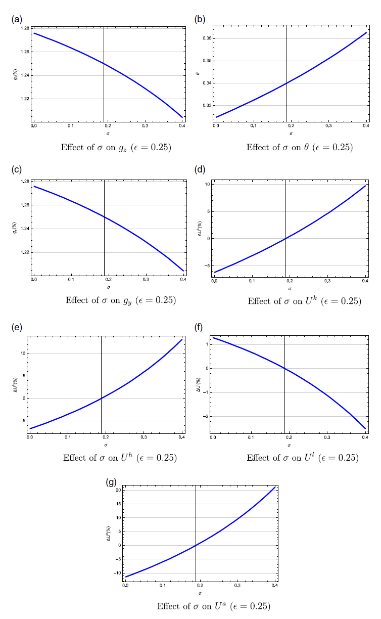
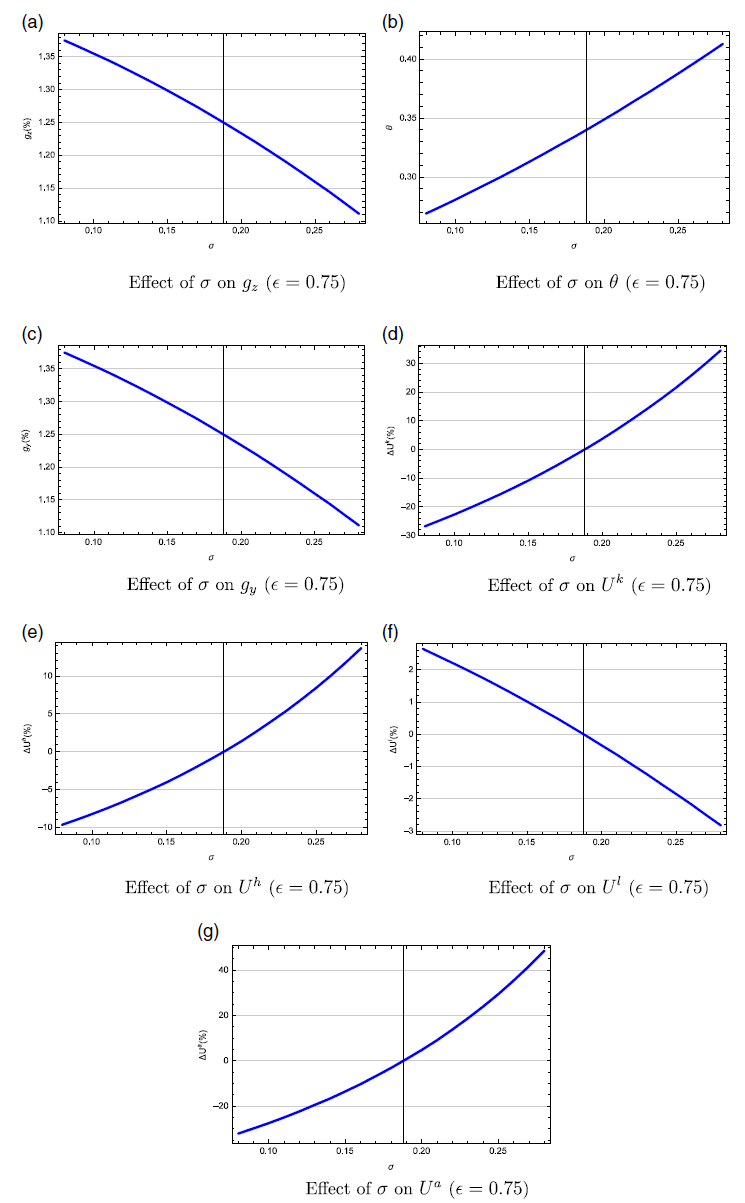
Figure 8 simulates the effects of automation subsidy
 $\sigma$
for the case of
 $\epsilon =0.25$
. Figure 9 simulates the effects of automation subsidy
 $\sigma$
for the case of
 $\epsilon =0.75$
. They show that the effects of automation subsidy
 $\sigma$
follow the same pattern across the whole range of values for
 $\epsilon \in \lbrack 0.25,0.75]$
.
a: Effect of
 $\sigma$
on
 ${g}_{z}$
(
 $\epsilon =0.25$
); b: Effect of
 $\sigma$
on
 $\theta$
(
 $\epsilon =0.25$
); c: Effect of
 $\sigma$
on
 ${g}_{y}$
(
 $\epsilon =0.25$
); d: Effect of
 $\sigma$
on
 ${U}^{k}$
(
 $\epsilon =0.25$
); e: Effect of
 $\sigma$
on
 ${U}^{h}$
(
 $\epsilon =0.25$
); f: Effect of
 $\sigma$
on
 ${U}^{l}$
(
 $\epsilon =0.25$
); and g: Effect of
 $\sigma$
on
 ${U}^{a}$
(
 $\epsilon =0.25$
).

a: Effect of
 $\sigma$
on
 ${g}_{z}$
(
 $\epsilon =0.75$
); b: Effect of
 $\sigma$
on
 $\theta$
(
 $\epsilon =0.75$
); c: Effect of
 $\sigma$
on
 ${g}_{y}$
(
 $\epsilon =0.75$
); d: Effect of
 $\sigma$
on
 ${U}^{k}$
(
 $\epsilon =0.75$
); e: Effect of
 $\sigma$
on
 ${U}^{h}$
(
 $\epsilon =0.75$
); f: Effect of
 $\sigma$
on
 ${U}^{l}$
(
 $\epsilon =0.75$
); and g: Effect of
 $\sigma$
on
 ${U}^{a}$
(
 $\epsilon =0.75$
).

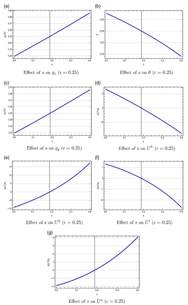
Effect of
 $s$
on
 ${g}_{z}$
(
 $\epsilon =0.25$
); b: Effect of
 $s$
on
 $\theta$
(
 $\epsilon =0.25$
); c: Effect of
 $s$
on
 ${g}_{y}$
(
 $\epsilon =0.25$
); d: Effect of
 $s$
on
 ${U}^{k}$
(
 $\epsilon =0.25$
); e: Effect of
 $s$
on
 ${U}^{h}$
(
 $\epsilon =0.25$
); f: Effect of
 $s$
on
 ${U}^{l}$
(
 $\epsilon =0.25$
); and g: Effect of
 $s$
on
 ${U}^{a}$
(
 $\epsilon =0.25$
).

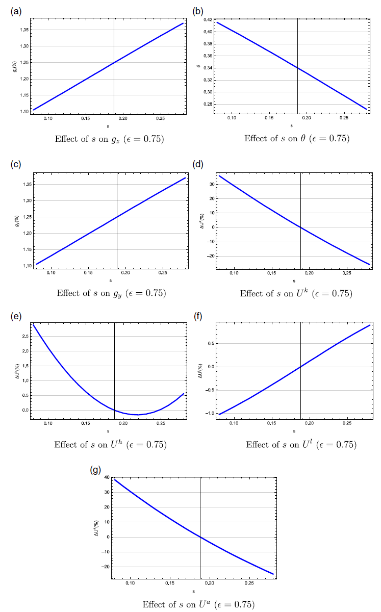
a: Effect of
 $s$
on
 ${g}_{z}$
(
 $\epsilon =0.75$
); b: Effect of
 $s$
on
 $\theta$
(
 $\epsilon =0.75$
); c: Effect of
 $s$
on
 ${g}_{y}$
(
 $\epsilon =0.75$
); d: Effect of
 $s$
on
 ${U}^{k}$
(
 $\epsilon =0.75$
); e: Effect of
 $s$
on
 ${U}^{h}$
(
 $\epsilon =0.75$
); f: Effect of
 $s$
on
 ${U}^{l}$
(
 $\epsilon =0.75$
); and g: Effect of
 $s$
on
 ${U}^{a}$
(
 $\epsilon =0.75$
).

Figure 10 simulates the effects of R&D subsidy
 $s$
for the case of
 $\epsilon =0.25$
. Figure 11 simulates the effects of R&D subsidy
 $s$
for the case of
 $\epsilon =0.75$
. Figure 10 shows that most effects of R&D subsidy
 $s$
follow the same pattern when the value of
 $\epsilon$
decreases from 0.50 to 0.25. However, Figure 11 shows that the effects of R&D subsidy
 $s$
become slightly different when the value of
 $\epsilon$
increases from 0.50 to 0.75. Specifically, Figure 11e shows that the effect of R&D subsidy
 $s$
on
 $U^{h}$
becomes U-shaped whereas Figure 11f shows that the effect of R&D subsidy
 $s$
on
 $U^{l}$
becomes positive. Intuitively, the high-skill workers become worse off by the higher tax rate but benefit from higher R&D subsidies, which together generate an overall U-shaped effect. As for the low-skill workers, the welfare gains from the higher growth rate and the higher share of production wage income dominate the higher tax burden in this case.
D. Appendix D: Capital income tax
In this appendix, we derive the equilibrium conditions under capital income tax in Section 4.1. By (14) and (42), the balanced-growth values of an innovation and an automation are
 \begin{eqnarray} v_{t}^{l} &=&\frac{\left ( 1-\tau \right ) \pi _{t}^{l}}{\tau g_{y}+\rho +\left ( 1-\tau \right ) \left ( \phi h_{a}^{\epsilon }+\varphi h_{r}^{\epsilon }\right ) }\text{,} \end{eqnarray}
 \begin{eqnarray} v_{t}^{k} &=&\frac{\left ( 1-\tau \right ) \pi _{t}^{k}}{\tau g_{y}+\rho +\left ( 1-\tau \right)\!\varphi h_{r}^{\epsilon }}\text{.} \end{eqnarray}
Substituting (D.1) and (D.2) into the free-entry conditions, (17) and (19), yields
 \begin{equation} \frac{\varphi (1-\sigma )h_{a}^{1-\epsilon }}{\phi (1-\theta )(1-s)h_{r}^{1-\epsilon }}=\frac{\tau g_{y}+\rho +\left ( 1-\tau \right ) \left ( \phi h_{a}^{\epsilon }+\varphi h_{r}^{\epsilon }\right ) }{\tau g_{y}+\rho +\left ( 1-\tau \right)\!\varphi h_{r}^{\epsilon }}\text{,} \end{equation}
which uses
 $h_{a}=1-h_{r}$
and
 $1-\theta =\varphi h_{r}^{\epsilon }/(\phi h_{a}^{\epsilon }+\varphi h_{r}^{\epsilon })$
. We can rewrite (D.3) as
 \begin{equation} \frac{1-\sigma }{1-s}\left [ \frac{\varphi }{\phi }+\left ( \frac{1-h_{r}}{h_{r}}\right ) ^{\epsilon }\right ] =\left ( \frac{h_{r}}{1-h_{r}}\right ) ^{1-\epsilon }+\left ( \frac{h_{r}}{1-h_{r}}\right ) ^{1-2\epsilon }\frac{\phi }{\varphi +\left ( \tau g_{y}+\rho \right )/\left [ \left ( 1-\tau \right)\!h_{r}^{\epsilon }\right ] }\text{,} \end{equation}
in which
 $g_{y}=\varphi h_{r}^{\epsilon }\ln z$
. If
 $\tau =0$
, (D.4) simplifies to (31); otherwise, (D.4) shows the presence of general-equilibrium effects from changes in the subsidy rate,
 $s$
or
 $\sigma$
, through
 $\tau$
and
 $g_{y}$
.
To determine the steady-state value of
 $\tau$
, we substitute (D.1) and (D.2) into
 $a_{t}=\theta v_{t}^{k}+\left ( 1-\theta \right ) v_{t}^{l}$
to derive
 \begin{equation} a_{t}=\left [ \frac{\theta }{\tau g_{y}+\rho +\left ( 1-\tau \right)\!\varphi h_{r}^{\epsilon }}+\frac{1-\theta }{\tau g_{y}+\rho +\left ( 1-\tau \right ) \left ( \phi h_{a}^{\epsilon }+\varphi h_{r}^{\epsilon }\right ) }\right ] \left ( 1-\tau \right ) \frac{\mu -1}{\mu }y_{t}\equiv \tilde{a}y_{t}\text{.} \end{equation}
With
 $R=r+\delta$
, (26) implies
 \begin{equation} k_{t}=\frac{\theta }{\mu }\frac{1}{r+\delta }y_{t}\equiv \tilde{k}y_{t}\text{,} \end{equation}
in which
 $r=\left ( g_{y}+\rho \right )/\left ( 1-\tau \right )$
. Then, substituting (D.5) and (D.6) into the government’s balanced-budget condition in (43) yields
 \begin{equation} \frac{y_{t}}{w_{h,t}}=\frac{sh_{r}+\sigma h_{a}}{(\tilde{a}+\tilde{k})\tau r}\text{.} \end{equation}
From (19), (28) and (D.2), we can derive
 \begin{equation} \frac{y_{t}}{w_{h,t}}=\frac{\mu }{\mu -1}\frac{(1-\sigma )h_{a}^{1-\epsilon }}{\phi\!\left ( 1-\tau \right ) (1-\theta )}\left [ \tau g_{y}+\rho +\left ( 1-\tau \right)\!\varphi h_{r}^{\epsilon }\right ] \text{.} \end{equation}
 \begin{eqnarray} &&\!\!\!\!\frac{\phi }{1-\sigma }\frac{1-\tau }{\tau }\frac{sh_{r}+\sigma\!\left(1-h_{r}\right ) }{\left ( g_{y}+\rho \right ) \left ( 1-h_{r}\right ) ^{1-\epsilon }} \\ &&\!\!\!\!=\frac{\tau g_{y}+\rho +\left ( 1-\tau \right)\!\varphi h_{r}^{\epsilon }}{\tau g_{y}+\rho +\left ( 1-\tau \right ) \left [ \varphi h_{r}^{\epsilon }+\phi\!\left ( 1-h_{r}\right ) ^{\epsilon }\right ] }+\frac{\phi }{\varphi }\left ( \frac{1-h_{r}}{h_{r}}\right ) ^{\epsilon }\left [ 1+\frac{1}{\mu -1}\frac{\tau g_{y}+\rho +\left ( 1-\tau \right)\!\varphi h_{r}^{\epsilon }}{g_{y}+\rho +\left ( 1-\tau \right)\!\delta }\right ] \text{.} \notag \end{eqnarray}
Note that (D.4) and (D.9), with
 $g_{y}=\varphi h_{r}^{\epsilon }\ln z$
, determine the steady-state values of
 $h_{r}$
and
 $\tau$
.
E. Appendix E: Automation-driven economic growth
In this appendix, we show that automation subsidy has an overall inverted-U effect on economic growth. Equation (31) shows that R&D labor
 $h_{r}$
is decreasing in automation subsidy
 $\sigma$
. Using (46), we obtain
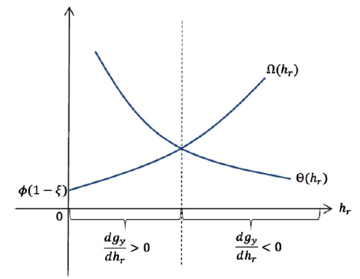
 \begin{equation} \frac{dg_{y}}{dh_{r}}=\epsilon \ln z\left [ \underset{\equiv \Theta (h_{r})}{\underbrace{\varphi h_{r}^{\epsilon -1}}}-\underset{\equiv \Omega (h_{r})}{\underbrace{\phi\!\left ( 1-\xi \right ) \left ( 1-h_{r}\right ) ^{\epsilon -1}}}\right ] \text{.} \end{equation}
Note the following properties:(a)
 $\Theta (h_{r})$
is a strictly decreasing function and
 $\Omega (h_{r})$
is a strictly increasing function; (b)
 $\Omega (0)=\phi\!\left ( 1-\xi \right )$
; (c) both
 $\Theta (h_{r})$
and
 $\Omega (h_{r})$
are strictly convex. Using these properties, we can graphically show that
 $\Omega (h_{r})$
intersects
 $\Theta (h_{r})$
from below only once at some point
 $h_{r}\in \left ( 0,1\right )$
, below (above) which
 $dg_{y}/dh_{r}>(<0)$
; see Figure 12. This result implies an inverted-U relation between
 $h_{r}$
and
 $g_{y}$
.
 $\Theta (h_{r})$
and
 $\Omega (h_{r})$
.