2. Stokes solution: a recapitulation

Figure 1.

(a) Flow round a corner between fixed planes $\theta =\pm \alpha$ with $\pi /2\lt \alpha \le \pi$ ; (b) schematic of flow around a cylinder of triangular cross-section driven by rotation of an outer circular cylinder; in this note, we are concerned only with the flow near the vertices A, B or C of the inner cylinder.

Figure 1. Long description

Panel A: Diagram of fluid flow around a corner between fixed planes. The diagram shows the flow lines converging and diverging around the corner. The flow lines are color-coded, with blue and red lines indicating the boundaries of the flow. The angles θ * α and θ * -α are marked, and arrows indicate the direction of flow. Panel B: Schematic of flow around a cylinder of triangular cross-section driven by rotation of an outer circular cylinder. The inner cylinder has vertices labeled A, B, and C. The flow lines form concentric circles around the triangular cylinder, with arrows indicating the direction of flow.

Consider first the two-dimensional flow round a sharp corner (i.e. one of zero radius of curvature) formed by two fixed planes $\theta =\pm \alpha$ with $\pi /2 \lt \alpha \le \pi$ , on which the no-slip condition is imposed. The situation is illustrated in figure 1(a). At the origin $r=0$ , the velocity $\boldsymbol {u}=(u_{r},u_{\theta })$ is zero, and we may therefore assume that the local Reynolds number based on distance $r$ from the corner is small, and fluid inertia is negligible. It is supposed that the flow is driven by some mechanism far from the corner. (Figure 1 b illustrates one possible example: this is Couette flow between two cylinders, with the inner cylinder of triangular cross-section fixed, and the flow being driven by rotation of the outer circular cylinder. Of course any inner cylinder of polygonal cross-section with interior angles less than $\pi$ would present similar problems. We are concerned here only with the flow in the immediate vicinity of any vertex of the inner cylinder.) For the situation considered here, with the angle $2\alpha$ in the reflex range $\pi \le 2\alpha \le 2\pi$ , the streamfunction $\psi (r,\theta )$ has the asymptotic form

(2.1) \begin{equation} \psi (r,\theta ) \sim \,r^{\mu +1}f(\theta , \alpha ) \quad \text{as}\quad r\rightarrow 0, \end{equation}

where the exponent $\mu$ depends on the angle $\alpha$ in a manner that must be determined. The velocity $\boldsymbol {u}=(u_r, u_\theta )$ is then given by

(2.2) \begin{equation} u_r= r^{-1}\partial \psi /\partial \theta = r^{\mu }\partial f/\partial \theta ,\,\quad u_\theta =- \partial \psi /\partial r =-(\mu +1) r^{\mu }f(\theta ,\alpha ). \end{equation}

For the case in which $u_r$ is antisymmetric about the bisector $\theta =0$ (as in figure 1 a), $f(\theta ,\alpha )$ is an even function of $\theta$ , and is given by

(2.3) \begin{equation} f(\theta ,\alpha ) = A\cos (\mu +1)\theta + B \cos (\mu -1)\theta . \end{equation}

Here, the scaling is arbitrary, and so the coefficient $A$ , say, is arbitrary (being in principle determined by the remote forcing conditions, here unspecified). The no-slip conditions are satisfied on $\theta =\pm \alpha$ provided

(2.4) \begin{equation} A\cos (\mu +1)\alpha + B \cos (\mu -1)\alpha = 0, \end{equation}

Figure 2.

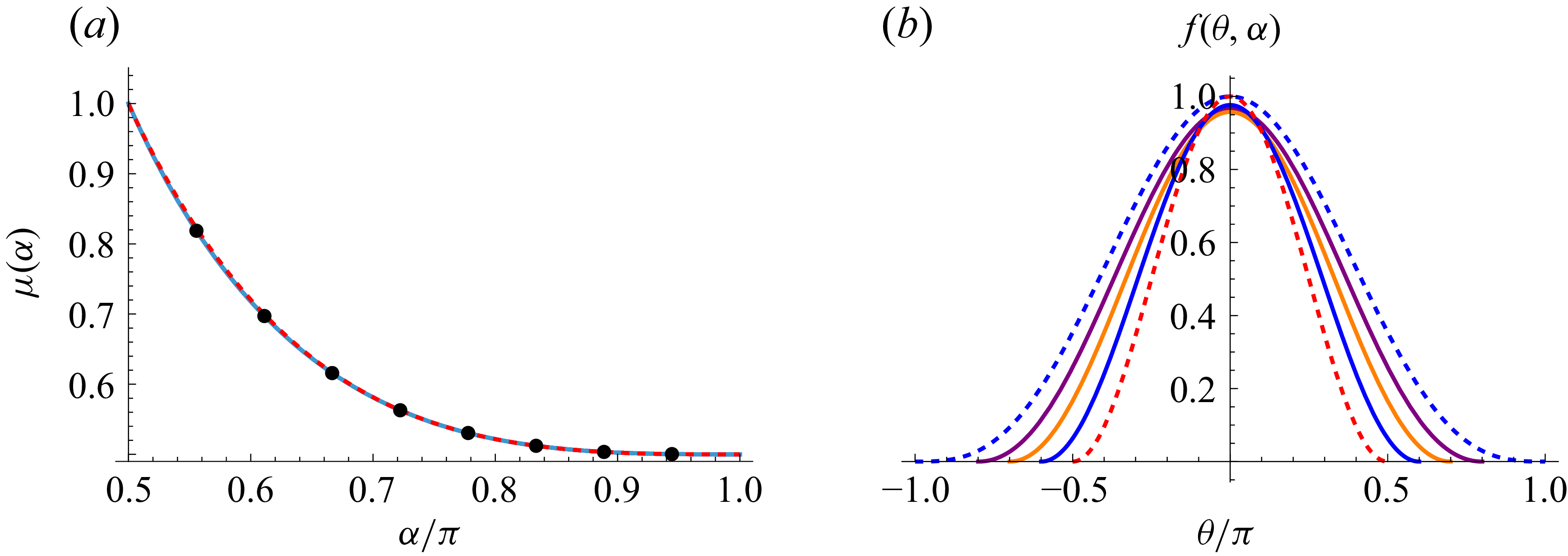
(a) The function $\mu (\alpha )$ over the range $1/2 \le \alpha /\pi \le 1$ (continuous blue curve); the red, dashed curve superposed on this is the three-term asymptotic function $\mu _{a}(\alpha )$ (2.10); the black points are as obtained by a graphical method by Dean & Montagnon (Reference Dean and Montagnon1949). (b) The function $f(\theta , \alpha )$ , given by (2.8), for $\alpha /\pi =0.5$ (red, dashed), $0.6$ (blue), $0.7$ (orange), $0.8$ (purple) and $1$ (blue, dashed).

and

(2.5) \begin{equation} A(\mu +1)\sin (\mu +1)\alpha +B(\mu -1) \sin (\mu -1)\alpha = 0. \end{equation}

For a non-trivial solution for $B/A$ , $\mu$ must then satisfy the transcendental equation

(2.6) \begin{equation} F(\alpha ,\mu )\equiv \sin {2\mu \alpha }+\mu \sin {2\alpha }=0, \end{equation}

and the condition of zero velocity at $r=0$ requires that $\mu \gt 0$ . When $\alpha =\pi /2$ , $\sin \pi \mu =0$ , and the smallest positive root is $\mu =1$ . For $\alpha \gt \pi /2$ , with $\mu =\mu (\alpha )$ determined as the smallest real positive root of (2.6), and with the convenient choice

(2.7) \begin{equation} A=\frac {\cos [(\mu -1)\alpha ]}{2\sin \alpha } \end{equation}

for the pre-factor $A$ , (2.3) then gives

(2.8) \begin{equation} f(\theta ,\alpha )=\sin \alpha \mu \cos \theta \cos \mu \theta - \cot \alpha \cos \alpha \mu \sin \theta \sin \mu \theta , \end{equation}

which remains bounded for all $\alpha \in [\pi /2,\,\pi ]$ . Figure 2(a) shows the function $\mu (\alpha )$ , obtained as the zero contour of the function $F(\alpha ,\mu )$ starting from the point $\alpha =\pi /2, \mu =1$ . Note that since ${\rm d}F=(\partial F/\partial \alpha ) {\rm d}\alpha +(\partial F/\partial \mu ) {\rm d}\mu =0$ , it follows that

(2.9) \begin{equation} \frac {{\rm d}\mu }{{\rm d}\alpha } =-\frac { \partial F/\partial \alpha }{\partial F/\partial \mu } =- \frac {2\mu (\cos 2 \alpha \mu + \cos 2 \alpha )} {2 \alpha \cos 2 \alpha \mu + \sin 2 \alpha }, \end{equation}

and so the curve of figure 2(a) may be obtained alternatively by numerical integration of (2.9) with starting condition $\mu (\pi /2)=1$ . Either way, the resulting function $\mu (\alpha )$ in figure 2(a) evidently decreases monotonically from 1 to 1/2 as $\alpha$ increases from $\pi /2$ to $\pi$ . The vorticity $\omega =-{\nabla} ^{2}\psi$ is proportional to $r^{\mu -1}$ , and is therefore singular at the vertex $r=0$ for all $\alpha \gt \pi /2$ . Analysis of (2.6) reveals the asymptotic form as $\alpha \rightarrow \pi$

(2.10) \begin{equation} \mu (\alpha )\sim \mu _{a}(\alpha )+\text{O} (\pi -\alpha )^6, \quad \text{where}\quad \mu _{a}(\alpha )= \frac {1}{2}+\frac {(\pi -\alpha )^3}{4\pi } + \frac {(\pi -\alpha )^5}{16\pi } . \end{equation}

The three-term asymptotic function $\mu _{a}(\alpha )$ is superposed (red, dashed) on $\mu (\alpha )$ in figure 2(a) and is fortuitously accurate over the whole range $1/2 \le \alpha /\pi \le 1$ (even at the lower limit, where $\mu _{a}(\pi /2)\approx 0.9987$ ). The black dots on this curve are at points obtained by Dean & Montagnon (Reference Dean and Montagnon1949) by a graphical procedure, and are also accurate to three significant figures, a fine achievement in the pre-computer age!

The function $f(\theta ,\alpha )$ (as given by (2.8)) is plotted in figure 2(b) for several values of $\alpha$ . In the limiting case $\alpha =\pi /2$ , $f(\theta ,\pi /2)= \cos ^{2} \theta$ (the red dashed curve in figure 2 b), and the flow is simply a uniform shear parallel to the plane boundary $x\, (=r\cos \theta ) =0$ .

The other limiting case $\alpha =\pi$ in which the ‘wedge’ of figure 1(a) collapses to a flat plat on $\theta =\pm \pi$ , requires special consideration. In this case, with $\alpha =\pi$ and $ \mu =1/2$ , equation (2.4) is identically satisfied, and (2.5) gives

(2.11) \begin{equation} -(3/2)A +(1/2)B =0. \end{equation}

Hence, taking $A=\textstyle { {1}/{4}} \displaystyle$ (the limit of (2.7) as $\alpha \rightarrow \pi$ ), equation (2.8) gives

(2.12) \begin{equation} f(\theta , \pi ) = \textstyle {\frac {1}{4}} \displaystyle [\cos (3\theta /2) +3 \cos (\theta /2)] = \cos ^{3} (\theta /2). \end{equation}

This is the blue dashed curve in figure 2(b).

2.1. Flow structure

We can now plot the streamlines $\psi (r,\theta )=r^{\mu (\alpha )+1}f(\theta ,\alpha )=$ const. Two examples are shown in figure 3, for $\alpha =0 .7\pi$ and $\alpha = 0.9\pi$ .

Figure 3.

Streamlines $\psi (r,\theta )=r^{\mu (\alpha )+1}f(\theta ,\alpha )=$ const. for (a) $\alpha =0.7\pi$ and (b) $\alpha =0.9\pi$ . Note how, in both cases, the streamlines converge with decreasing distance from the vertex. Arrows on the streamlines are not included, since Stokes flows, with negligible inertia, are reversible.

Figure 3. Long description

Two graphs labeled (a) and (b) depict streamlines converging towards a vertex. Each graph is a plot of streamlines, which are lines that represent the paths taken by particles in a fluid flow. The horizontal and vertical axes are not labeled with specific units or ranges, indicating a focus on the qualitative behavior of the streamlines. In both graphs, the streamlines converge as they approach the vertex located at the origin (0,0). The streamlines in both graphs are color-coded: blue, cyan, orange, and green. The blue streamlines are closest to the vertex, followed by cyan, orange, and green streamlines, which are progressively farther from the vertex. The convergence of streamlines indicates that the velocity of the fluid increases as it approaches the vertex. No arrows are included on the streamlines, as the flow is reversible due to negligible inertia. Panel A and Panel B show similar patterns of streamline convergence, highlighting the consistent behavior of the fluid flow in different scenarios.

Figure 4.

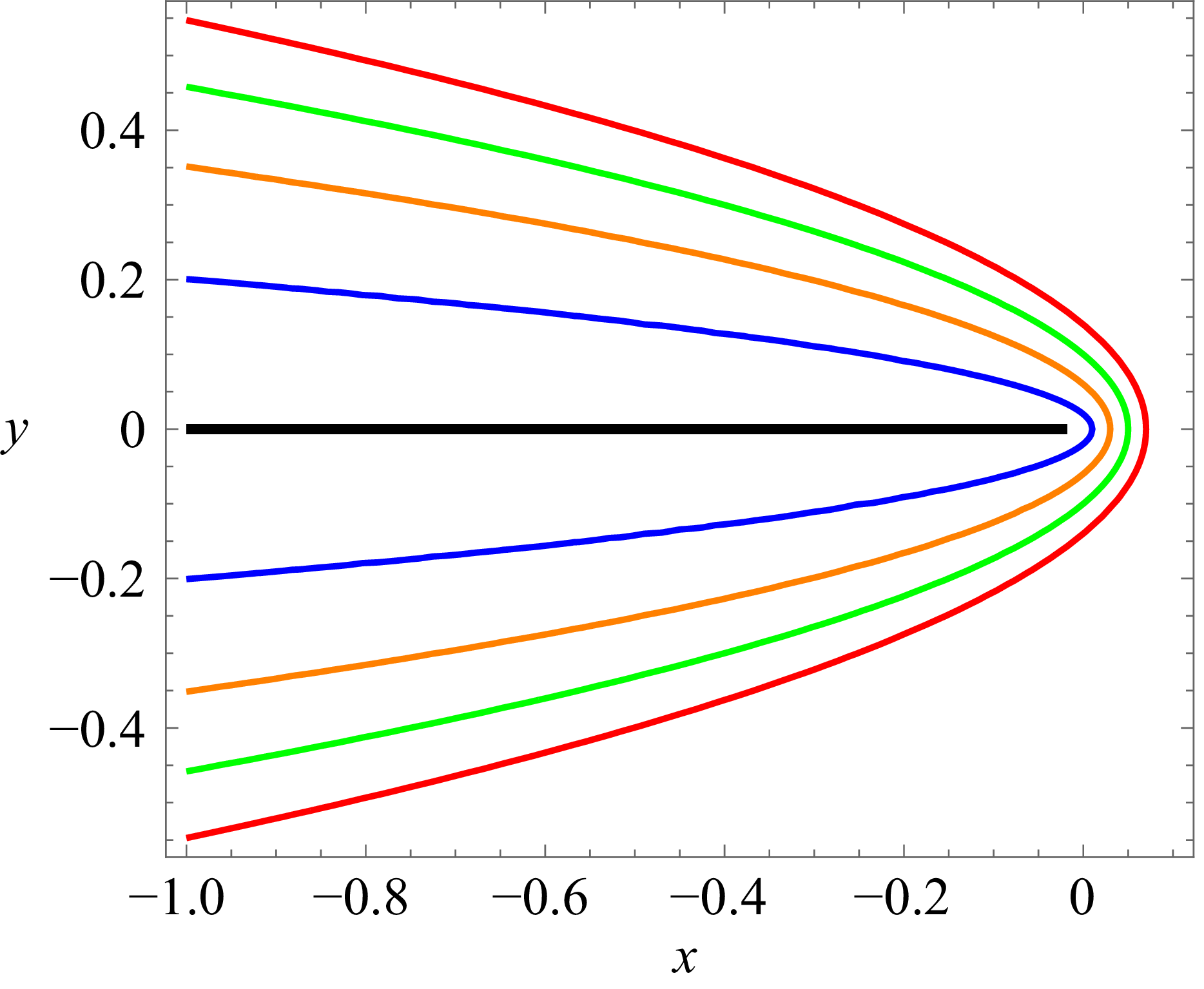
Parabolic streamlines in the flat-plate limit $\alpha =\pi$ , with $\psi (r,\theta )=[\textstyle {({1}/{2})} \displaystyle r(1+\cos \theta )]^{3/2}$ .

In the limiting case $\alpha =\pi$ , the streamfunction is given by

(2.13) \begin{equation} \psi (r,\theta )=r^{3/2}\cos ^{3} (\theta /2) =\big [r\cos ^{2}(\theta /2)\big]^{3/2}=\left [\textstyle {\frac {1}{2}} \displaystyle r(1+\cos \theta )\right ]^{3/2}\!. \end{equation}

Hence, with $x=r\cos \theta$ , the streamline $\psi = \psi _{0}$ (const.) is the parabola

(2.14) \begin{equation} r+x= 2 \psi _{0}^{2/3} =2 a,\,\,\text{say}, \end{equation}

or equivalently

(2.15) \begin{equation} y^2= 4a(a-x). \end{equation}

The family of parabolic streamlines (for varying $a$ ) is shown in figure 4.

2.2. Acceleration along streamlines as the corner region is approached

It is evident from figures 3 and 4 that the streamlines invariably converge when approaching the corner, indicating acceleration with decreasing distance from the vertex $r=0$ . At first sight, this appears paradoxical as the velocity $|\boldsymbol {u} |$ is proportional to $r^{\mu (\alpha )}$ which tends to zero for all $\alpha$ in the range $\pi /2\lt \alpha \le \pi$ . It is a situation in which we apparently have fluid particles accelerating with decreasing distance from the stagnation point at the vertex! In this respect, the sketch of figure 4(a) of Moffatt (Reference Moffatt1964) is, however, misleading; we take the opportunity to correct this here.

The paradox arises because, although the decrease of velocity to zero occurs on radial lines $\theta =$ const., it does not do so on streamlines as may be shown as follows. From (2.2), we have

(2.16) \begin{equation} {| \boldsymbol {u}}|= \big [u_{r}^2+u_{\theta }^2\big]^{1/2} = r^{\mu (\alpha )} \big [(\partial f/\partial \theta )^{2}+(\mu +1)^{2}f^{2}(\theta ,\alpha )\big ]^{1/2} . \end{equation}

We may evaluate this on any streamline $\psi =\psi _0$ , on which $r= [\psi _{0}/f(\theta ,\alpha )]^{1/(1+\mu (\alpha ))}$ . On such a streamline

(2.17) \begin{equation} |{ \boldsymbol {u}}(\theta , \alpha )|=c \big [(\partial f/\partial \theta )^{2}+(\mu +1)^{2}f^{2}(\theta ,\alpha )\big ]^{1/2} f(\theta ,\alpha )^{-\mu (\alpha )/[1+\mu (\alpha )]}, \end{equation}

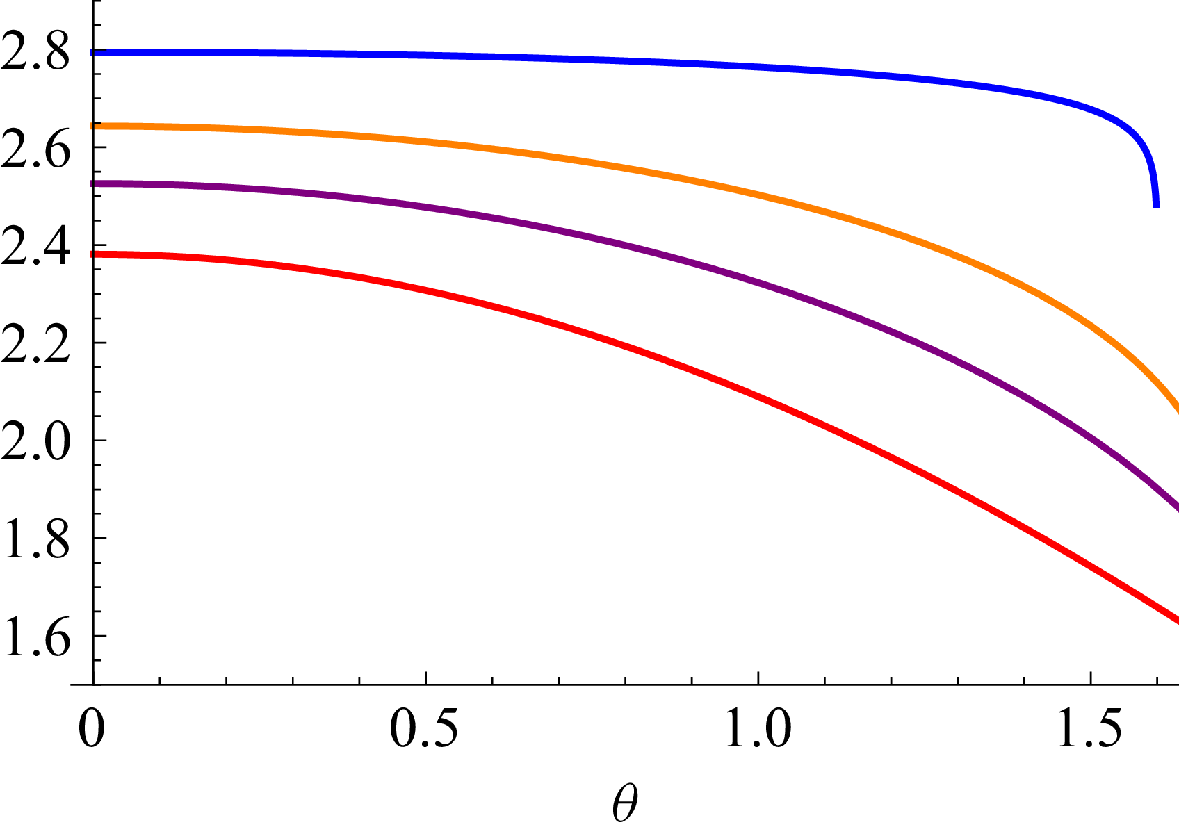
where $c= \psi _{0}^{\mu (\alpha )/[\mu (\alpha )+1]}$ . The expression $c^{-1}|{\boldsymbol {u}}(\theta , \alpha )|$ is plotted in figure 5 for $0\lt \theta \lt \pi /2$ , for various values of $\alpha$ . As expected, in every case, the speed increases as $\theta$ decreases towards zero, so that any fluid particle does indeed accelerate as its distance $r$ from the vertex decreases. The dependence of $|{\boldsymbol {u}}|$ on $\theta$ in (2.16) evidently more than compensates the decrease due to the factor $r^{\mu (\alpha )}$ . (In the limiting case $\alpha =\pi$ with $\mu =1/2$ , the expression (2.17) evaluates explicitly to the function $(3/2^{5/6})\sqrt {1+\cos \theta }$ , monotonic over the range $0\lt \theta \lt \pi$ .)

Figure 5.

The behaviour of $c^{-1}|\boldsymbol {u}(\theta ,\alpha )|$ on any streamline $\psi =\psi _0$ over the range $0\lt \theta \lt \pi /2$ , for $\alpha = 0.51\,\pi$ (blue), $0.56\,\pi$ (orange), $0.60\,\pi$ (purple) and $\pi$ (red). In every case, the curves are monotonically increasing as $\theta$ decreases towards 0.

Figure 6.

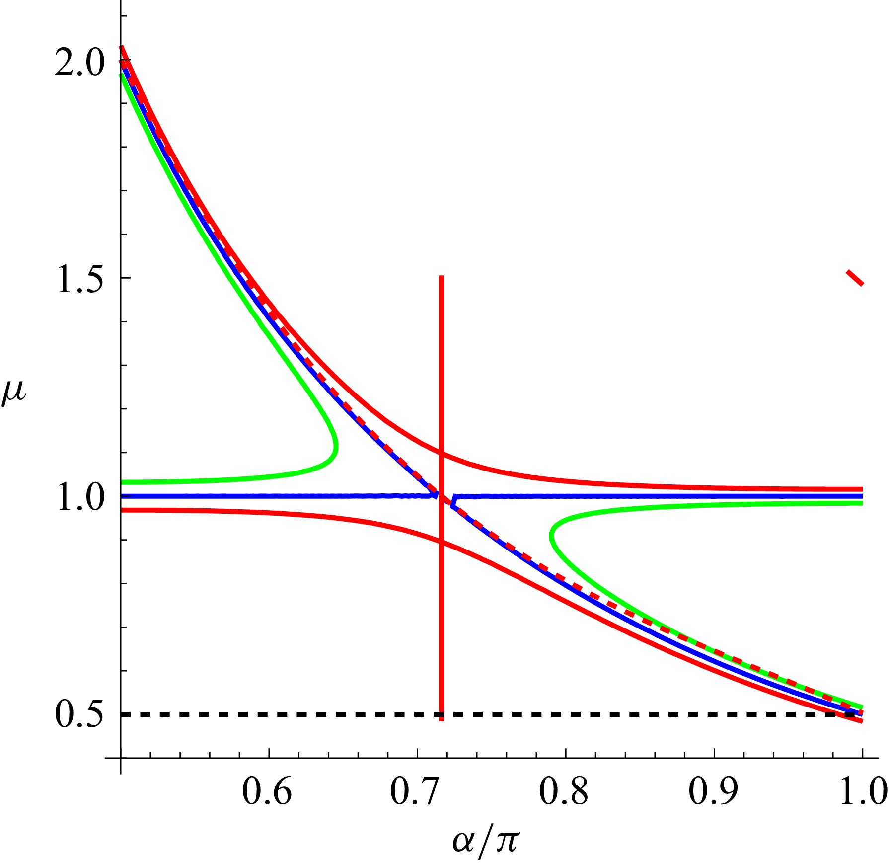
Contour $G(\alpha , \mu )=0$ (blue) for $\pi /2\le \alpha \le \pi$ ; the (dashed, red) curve $\mu =\mu _a(\alpha )$ given by (3.3) is superposed, indicating reasonable coincidence over the full range. Also shown are the contours $G(\alpha , \mu )=-0.1$ (green) and $+0.1$ (red). The zero contour crosses the line $\mu =1$ at $\alpha =\alpha _{c}$ as indicated by the red vertical line; $\alpha _{c}$ is the root of $\tan {2\alpha }=2\alpha$ in this range, i.e. $2\alpha _{c} \approx 1.43\pi \approx 257^{o}$ .

3. Flow symmetric about $\theta =0$

Consider now the complementary situation of flow symmetric about $\theta =0$ , as shown in figure 8(a,b) below. This is again a Stokes flow, and the flow can be either towards or away from the vertex of the wedge. An important example is the flow (relative to the body) near the leading edge of any sharp-tipped cylindrical body moving into a fluid at rest ‘at infinity’. The local streamfunction is now antisymmetric in $\theta$ and has the form

(3.1) \begin{equation} \psi (r,\theta )\sim r^{\mu +1}g(\theta ,\alpha )=r^{\mu +1}[C\sin (\mu +1)\theta +D\sin (\mu -1)\theta ], \end{equation}

and the no-slip conditions on $\theta =\pm \alpha$ are now satisfied provided

(3.2) \begin{equation} G(\alpha ,\mu )\equiv \sin 2\mu \alpha -\mu \sin 2\alpha =0. \end{equation}

Note first that this is identically satisfied for all $\alpha$ if $\mu =1$ ; however, equation (3.1) then gives $g(\theta ,\alpha )=C\sin 2\theta$ , and the no-slip conditions can be satisfied only if $C=0$ . The possibility $\mu =1$ thus yields only the trivial solution, and can be safely ignored (but see below).

Figure 7.

(a) The function $g(\theta ,\, \alpha )$ , given by (3.5), over the range $\alpha \le \theta \le \alpha$ for $\alpha /\pi =0.5$ (blue), $0.6$ (blue, dashed), $0.7$ (green), $0.8$ (green, dashed), $0.9$ (red) and $1$ (red, dashed); (b) three-dimensional plot of the same function over the range $\{\pi /2\lt \alpha \lt \pi , -\alpha \lt \theta \lt \alpha \}$ ; note that the function $g(\theta ,\, \alpha )$ extends continuously over the gap at $\alpha = \alpha _{c} \approx 0.715\pi$ , where the quotient (3.5) is indeterminate; the blue curve on this plot, given by (3.6), fills the ‘criticality’ gap $0.71\lt \alpha /\pi \lt 0.72$ .

From (3.2), when $\alpha =\pi /2$ , $\sin \pi \mu =0$ , so the next possibility with $\mu \gt 0$ is $\mu =2$ . The contour $G(\alpha ,\mu )=0$ starting from the point $\alpha =\pi /2,\,\mu =2$ is shown in figure 6. The required function $\mu (\alpha )$ is given by the curved part of this contour, which crosses the line $\mu =1$ at $\alpha =\alpha _{c}$ (indicated by the vertical red line); the ‘critical angle’ is $\alpha _{c} \approx 0.175\pi$ , as determined in the following paragraph. We include also the contours $G(\alpha ,\mu )=-0.1$ (green) and $+0.1$ (red) to indicate the structure near the critical point $\{\mu =1,\,\alpha =\alpha _{c}\}$ . We have also superposed on the zero contour the red dashed curve (obtained by simple curve fitting)

(3.3) \begin{equation} \mu =\mu _{a}(\alpha ) = 2-2.21(\alpha -\pi /2) +1.303(\alpha -\pi /2)^{2} -0.32(\alpha -\pi /2)^{3}, \end{equation}

which evidently provides a reasonable approximation over the whole range $\pi /2 \le \alpha \le \pi$ . In particular, $\mu _{a}(\alpha _c)= 1.00$ .

Just as for equation (2.9) above, we now have for the symmetric case

(3.4) \begin{equation} \frac {\text{d}\mu }{\text{d}\alpha } =-\frac { \partial G/\partial \alpha }{\partial G/\partial \mu } =- \frac {2\mu (\cos 2\mu \alpha - \cos 2 \alpha )} {2 \alpha \cos 2 \mu \alpha - \sin 2 \alpha }. \end{equation}

Here, obviously the numerator $\partial G/\partial \alpha =0$ on $\mu =1$ . Also, the denominator $\partial G/\partial \mu = 2\alpha \cos 2\mu \alpha -\sin 2\alpha$ vanishes on the line $\mu =1$ where $\tan 2\alpha = 2\alpha$ , i.e. at $\alpha =\alpha _{c}\approx 2.247=0.715\pi$ , or equivalently $2\alpha _{c}\approx 257^{o}$ . Hence the expression (3.4) for $\text{d}\mu /\text{d}\alpha$ is indeterminate at the critical point $\{\alpha =\alpha _c,\,\mu =1\}$ . The angle $\alpha _c$ has been previously recognised by Moffatt & Duffy Reference Moffatt and Duffy1980 as the angle at which, in the context of flow driven by hinged plates in relative angular motion, a changeover occurs in the behaviour near the corner from that described by a local similarity solution $\psi \sim r^2$ when $\alpha \lt \alpha _c$ to that determined by remote conditions and described by the leading term of an asymptotic expansion $\psi \sim r^{\mu (\alpha )+1}$ when $\alpha \gt \alpha _c$ .

With $\mu (\alpha )$ determined, and $D =-C\sin [\alpha (\mu (\alpha )+1)]\csc [\alpha (\mu (\alpha )-1)]$ , the function $ g(\theta ,\alpha )$ in (3.1) may now be obtained. Choosing $C=-1/(2\sin \alpha )$ , (cf. the freedom of choice for $A(\alpha )$ in (2.7)), we find

(3.5) \begin{equation} g(\theta ,\alpha )=\frac {\cos [\alpha \, \mu (\alpha )]\cos \theta \sin [\theta \, \mu (\alpha )]-\cot \alpha \sin [\alpha \,\mu (\alpha )]\sin \theta \cos [\theta \,\mu (\alpha )]}{\sin [\alpha (\mu (\alpha )-1]}. \end{equation}

The numerator in this expression is identically zero (for all $\theta$ ) when $\mu (\alpha )=1$ , i.e. when $\alpha =\alpha _c$ . This is, however, compensated by the zero of the denominator at $\mu (\alpha )=1$ . Adopting the approximation (3.3), $\mu (\alpha ) \approx \mu _{a}(\alpha )$ , the function (3.5) has been plotted over the range $-\alpha \le \theta \le \alpha$ , as shown in figure 7(a) for $\alpha /\pi =0.5, 0.6, 0.7, 0.8, 0.9, 1$ . The three-dimensional plot of figure 7(b) shows that this family of curves passes smoothly through the critical point at $\alpha =\alpha _c\approx 0.715\pi$ . The blue curve on this plot fills the ‘criticality’ gap $0.71\lt \alpha /\pi \lt 0.72$ and is given to good approximation by the equation

(3.6) \begin{equation} g(\theta , \alpha _{c}) \approx -\textstyle {\frac {1}{2}} \displaystyle [\theta /\alpha _{c} +\sin 2\theta ],\qquad \{-\alpha _{c}\lt \theta \lt \alpha _{c}\}. \end{equation}

Figure 8.

Streamlines $\psi =$ const. for (a) $\alpha =0.6\,\pi$ and (b) $\alpha =0.9\,\pi$ . When the flow is directed from the right towards the vertex, the divergence of the streamlines indicates Lagrangian retardation of fluid particles.

Figure 8. Long description

Panel A: This graph shows streamlines for a flow symmetric about a vertex. The horizontal axis ranges from -4 to 6, and the vertical axis ranges from -4 to 4. The streamlines are represented by different colored curves. The flow is directed from the right towards the vertex, and the divergence of the streamlines indicates Lagrangian retardation of fluid particles. The blue shaded area on the left side of the graph indicates a region of interest. Panel B: This graph also shows streamlines for a flow symmetric about a vertex, but with a different configuration. The horizontal axis ranges from -6 to 6, and the vertical axis ranges from -6 to 6. The streamlines are represented by different colored curves. The blue shaded area on the left side of the graph indicates a region of interest. The flow is directed from the right towards the vertex, and the divergence of the streamlines indicates Lagrangian retardation of fluid particles.

Figure 9.

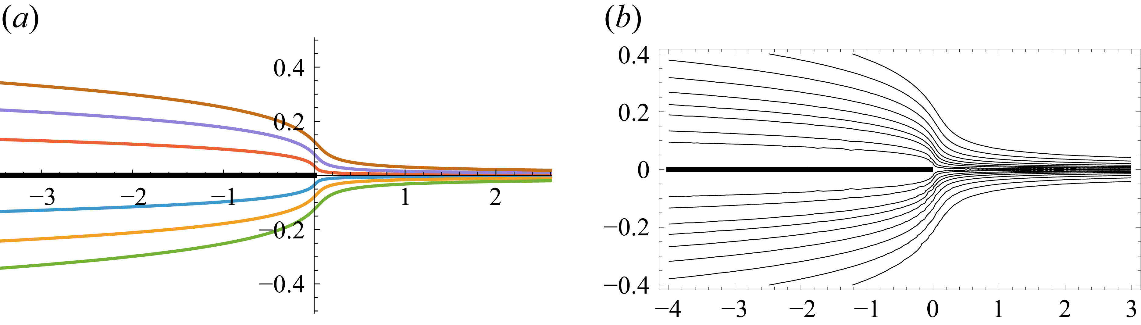
(a) Streamlines $\psi \propto r^{3/2}(1+\cos {\theta })\sin (\theta /2)=$ const. in the limiting situation $\alpha =\pi$ ; (b) more detailed contour plot of streamlines from the equivalent Cartesian form, $\psi \propto [(x^2 +y^2)^{1/2}+x]^{1/2}y$ .

Streamlines $\psi =$ const. for the cases $\alpha /\pi =0.6$ and $0.9$ are shown in figure 8(a,b). These are plotted using (3.1) (and (3.3) for $\mu (\alpha )$ ). In both cases it may be noted that the streamlines diverge approaching the vertex from the right, indicating (as might be expected in this case) deceleration of fluid particles on each streamline. (Again, arrows are not included on the streamlines, as the flows are in all cases reversible.)

Finally, figure 9(a) shows the limiting situation $\alpha =\pi ,\,\mu (\alpha )=1/2$ ; in this case, the limiting form of the streamfunction is

(3.7) \begin{equation} \psi (r,\theta )=r^{3/2}g(\theta ,\pi ) \sim -r^{3/2}(1+\cos {\theta })\sin (\theta /2), \end{equation}

a solution of the Stokes equation originally identified by Carrier & Lin (Reference Carrier and Lin1948) in their study of the boundary-layer flow on a flat plate. The equivalent Cartesian streamfunction is

(3.8) \begin{equation} \psi (x,y) \sim -\big[(x^2 +y^2)^{1/2}+x\big]^{1/2}y, \end{equation}

with contour plot showing essentially the same streamlines in greater detail in figure 9(b).

4. Asymmetric flow in the flat-plate limit $\alpha =\pi$

Figure 10.

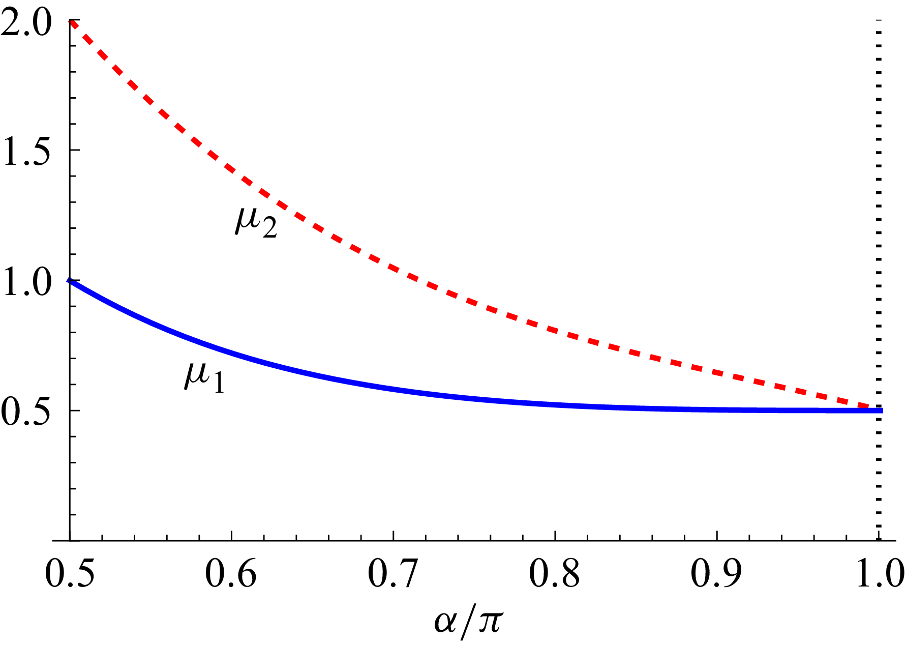
The functions $\mu _{1}(\alpha )$ and $\mu _{2}(\alpha )$ satisfying $F(\mu ,\alpha )=0$ and $G(\mu ,\alpha )=0$ respectively, showing that $\mu _{1}(\alpha )\le \mu _{2}(\alpha )$ , with equality only at the limit $\alpha =\pi$ .

Figure 11.

Streamlines $\psi =\psi _{0}$ for the streamfunction (4.1), with values of the constant $\psi _{0}$ on each streamline as marked; (a) $k=0.2$ ; (b) $k=0.5$ ; (c) $k=1.0$ ; (d) $k=5.0$ .

The relevant roots $\mu _{1}(\alpha )$ and $\mu _{2}(\alpha )$ for the two cases of antisymmetric and symmetric flow are replicated again in figure 10, showing that $\mu _{1}(\alpha )\le \mu _{2}(\alpha )$ with equality only in the limiting flat-plate situation $\alpha =\pi$ . In this limiting situation, any linear combination of the two flows (2.13) and (3.7) is a possible limiting solution of the Stokes equation ${\nabla} ^{4}\psi =0$ satisfying the no-slip conditions on both sides of the plate $\theta =\pm \pi$ . In Cartesian coordinates, such a linear combination may be written as an expression, homogeneous in $\{x, y \}$ of degree $3/2$

(4.1) \begin{equation} \psi (x,y; k)= \big [(x^2 +y^2)^{1/2}+x\big ]^{1/2}\big [(x^2 +y^2)^{1/2}+x+ky \big ], \end{equation}

for arbitrary constant $k$ . With this choice, note the obvious symmetry $\psi (x,y; -k)=\psi (x,-y; k)$ .

Four sets of streamlines $\psi (x,y; k)=$ const. are shown in figure 11, for $k= 0.2,0.5,1.0$ and $5.0$ . These are the asymptotic forms of flow near the leading edge of the plate, where the parameter $k$ is determined by remote conditions. Note how the separating streamline $\psi =0$ rotates anticlockwise as $k$ increases, asymptoting to $\theta =0$ for large $k$ (as in figure 9), when the rotating contribution to (4.1) is relatively weak.