World War II and its aftermath forcefully uprooted millions of Europeans.Footnote 1 During the war, Nazi Germany deported millions of people to die in concentration camps and millions of others to labor for the German war effort. Likewise, the Soviet Union deported hundreds of thousands of individuals from annexed territories (for example, the Baltic States and parts of Poland) to the Gulag labor camps and to exile settlements in Central Asia and Siberia. The war's end did not stop forced displacements. The major territorial changes that followed 1945 were accompanied by forced population transfers to increase ethnic homogeneity within the new borders. Poles had to leave former eastern territories of Poland (annexed by the Soviet Union), and Italians were expelled from Dalmatia and parts of Istria (annexed by Yugoslavia). The largest forced resettlement after World War II, and one of the largest such movements in human history,Footnote 2 involved Germans from East and Central Europe.
At least 12 million Germans fled or were expelled, most of them from the eastern territories of pre-World War I Germany and the Sudetenland. This huge inflow of expellees (Heimatvertriebene) drastically increased the population of what was about to become the Federal Republic of Germany (henceforth West Germany), from 39 million in 1939 to 48 million in 1950. By then, every sixth West German resident was an expellee.
The economic integration of expellees was a major challenge for the war-ridden country. Allied bombing campaigns had destroyed large parts of West Germany's housing stock, many industrial centers laid in ruins, and the labor market was in disarray. As a consequence, employment along with housing was a major source of conflict between expellees and the naive West German population. In fact, natives often viewed the newcomers as a threat to their economic interests and living standards (Connor Reference Connor2007). This article studies the effect of the expellee inflows on native employment to decide whether the fears of natives over job losses were indeed justified.
The displacement of Germans from East and Central Europe occurred in three distinct phases from 1944 to 1950. In the first phase, hundreds of thousands Germans fled westward at the final stages of the war to escape the approaching Red Army. These refugees predominately sought shelter in the nearest West German regions. Then, after the May 1945 fall of the Nazis, Polish and Czech authorities began to drive their remaining German populations out. The third phase followed the signature of the Treaty of Potsdam in August 1945. The treaty divided the former eastern territories of pre-World War II Germany between Poland and the USSR. Germans remaining east to the new border were brought to postwar Germany in compulsory and organized transfers. Attempts to rebalance the regional distribution of expellees were frustrated by deficient administrative structures and the French refusal to admit any expellees into their occupation zone. As a result, the regional distribution of expellees was very unequal when expulsions finally ended in 1950. At that time, the share of expellees in the population ranged from 5 percent in the state of Rhineland-Palatinate to 33 percent in Schleswig-Holstein.
Our analysis exploits this massive, sudden, and highly unequal increase in the labor force to study the effects on the employment-to-labor-force-rate (henceforth employment rate) of native West Germans using census data from September 1950. We break up the national labor market both by states and by occupations following David Card (Reference Card2001). As nearly all the Germans who lived in regions east to the new German border were forced to leave, the skill composition of immigrants was unusually rich. Natives in every occupation had to compete with expellees, but to quite varying degrees. Moreover, because inflow rates differed so much across labor market segments, we test for both a linear and a nonlinear relationship between native employment and expellee inflows.
While empirical analyses of the labor market effects of immigrationFootnote 3 are usually fraught with problems (Dustmann, Glitz, and Frattini Reference Dustmann, Glitz and Frattini2008), our specific historical setting simplifies the analysis. First, unlike in many other cases, expellees were close to perfect substitutes to native workers.Footnote 4 They all spoke German as their mother tongue and they had been educated in German schools. It thus seems reasonable that within a labor market segment, which we define by occupation and state (Bundesland), expellees and native West Germans were direct competitors. Second, endogenous location choices into thriving labor market segments should be of little importance for our case. Unlike voluntary migration, where individual decisions reflect the demand for skills in the origin and destination countries, expellees were not selected on the basis of their skills or attributes. Expellees were forced to relocate and few of them could choose their initial destination in West Germany. They either fled to regions close to their old homelands or, after the end of the war, were brought to West Germany in compulsory transfers. Once they had arrived in the West, their geographic mobility was severely restricted by law. Our setting is thus close to a natural experiment, in which immigrant inflows are independent of local labor market conditions. To address remaining endogeneity concerns, we complement OLS estimates with an instrumental variable strategy. Our instrument exploits regional variation in the prewar distribution of occupations and uses geographic proximity to predict expellee flows from the home regions of expellees to destination regions in West Germany.
Compared to most other immigration episodes, the mass arrival of expellees in postwar Germany arguably comes close to a worst-case scenario for natives as far as (short-run) employment effects are concerned.Footnote 5 Native workers had to compete against very similar migrant workers. In addition, migrants did not choose to immigrate because of favorable labor market conditions but were forced to relocate en masse to a war-ridden country. Indeed, we find that the inflow of expellees considerably reduced employment rates of native West Germans.Footnote 6 A 10 percentage point increase in the expellee share in a state-occupation cell decreased the employment rate of natives in the same cell by 4 percentage points. However, despite the initially dire labor market prospects in postwar Germany, expellee inflows had no effect on native employment as long as the expellee share did not exceed a level of about 15 percent. Only beyond that threshold did expellee inflows reduce native employment. To the best of our knowledge, we are the first to document such a nonlinear relation between native employment and immigrant inflows. It suggests that the West German labor market could absorb some expellee inflow without adverse employment effects on natives, but that absorption capacity was limited.
HISTORICAL BACKGROUND
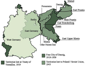
Henceforth, we will refer to those territories east of the current eastern border of Germany that were part of Germany prior to World War I as eastern territories (see Figure 1 for an overview of Germany's losses between 1919 and 1945). The eastern territories therefore include those regions that Germany lost in 1919 as well as those lost in 1945. The Sudetenland, which had been annexed from Czechoslovakia in September 1938, is not included (even though our empirical analysis will account for expellees from the Sudetenland). We refer to the Federal Republic of Germany as West Germany, and to the German Democratic Republic as East Germany (even before their formal creation in 1949). Together, West and East Germany represent the territory of current-day Germany.
GERMANY'S TERRITORIAL LOSSES, 1919–1945

The mass displacement of Germans from Eastern Europe occurred in three main phases (for further details, see Connor Reference Connor2007; Douglas Reference Douglas2012; Schulze Reference Schulze, Reinisch and White2011). The first phase began in July 1944 when Hitler allowed East Prussian authorities to organize a limited evacuation of women and children in the face of advancing Soviet troops. To prevent early territorial losses in the East, however, the Nazis delayed large-scale evacuations until January 1945 (Noble Reference Noble2006). As a result, the evacuations often started too late, if at all, and instead Germans fled en masse from the eastern front lines. In an attempt to stiffen the war effort, Nazi propaganda widely publicized Soviet atrocities, which only added to the population's panic. People rushed for the last trains or ships out of the territories under attack, and in many cases they fled on foot. Their escape routes were determined by the movement of the front. People from East Prussia, for instance, fled along the coast or boarded ships to North Germany as Soviet troops pushed westwards towards Berlin (Müller and Simon Reference Müller, Simon, Lemberg and Edding1959). Many refugees initially planned to return home after the end of the war, and some did so following Nazi Germany's May 1945 surrender. However, the Polish military soon stopped German refugees from returning to their former homes and turned them away at the Oder-Neisse line.
Starting in May 1945 authorities in Poland, soon followed by those in Czechoslovakia, began to expel the remaining German populations. These expulsions are known as “wild” because they were not sanctioned by an international agreement. They mark the second phase of the displacement. Germans were typically forced out of their homes on short notice, brought to holding camps to be shipped to occupied Germany by train or driven directly across the border. The Polish and Czech governments in exile had advocated the expulsions of German minorities since the beginning of the war. Their position was a direct response to Hitler's use of these minorities to grab first the Sudetenland and later parts of Poland. Although the Allies had agreed to the principle of such displacements before the end of the war, the wild expulsions were a way to create facts on the ground (Douglas Reference Douglas2012). And these “facts” could not be ignored when the Potsdam Conference convened in July of 1945.
The conference ended with the Treaty of Potsdam (August 2, 1945). In it, the United States, the United Kingdom, and the Soviet Union agreed to shift the border between Poland and Germany westwards to the Oder-Neisse line. Germany west to the Oder-Neisse line was divided into British, French, American, and Soviet zones of occupation. Poland, which lost a large part of its interwar territory to the Soviet Union, acquired Silesia, the eastern parts of Pomerania and Brandenburg, and most of East Prussia. The rest of East Prussia went to the Soviet Union (see Figure 1). These territories had nearly 10 million inhabitants and accounted for about 24 percent of Germany's area in 1937.
The Treaty of Potsdam also legalized the expulsions of Germans from Eastern Europe. It affirmed “that the transfer to [postwar] Germany of German populations, or elements thereof, remaining in Poland, Czechoslovakia, and Hungary, will have to be undertaken.” The agreement called for a temporary suspension of the expulsions until the Allied Control Council would agree on a plan to conduct the resettlement “in an orderly and humane” manner. Nevertheless, unauthorized expulsions continued until the end of 1945. On November 20 1945 the Allied Control Council announced a plan for the organized population transfers, and the third phase of the displacement began. The plan provided a timeline for moving the estimated 6.65 million Germans that were still living in Poland, Czechoslovakia, and Hungary, and set quotas for the expellee intake of each occupation zone. Most of the organized expulsions took place in the course of 1946. People were allowed to collect a few personal belongings, and were then either brought to an internment camp to await further transport or immediately put on often overloaded trains. In violation of official regulations, the transfers often separated families, as productive men were typically the last to be expelled. Expulsions continued, though on a much smaller scale, in the years after 1946.Footnote 7
Overall Size and Regional Distribution
By September 1950, when the mass displacement had finally come to an end, every sixth West German was an expellee.Footnote 8 Most expellees (55 percent or 4.4 million) came from the eastern provinces that Germany lost after World War II. Another 1.9 million expellees had lived in Czechoslovakia before the war, predominantly in the Sudetenland. The remaining expellees came mostly from the eastern territories that Germany had lost after its defeat in World War I, such as West Prussia, Posen, and Danzig.
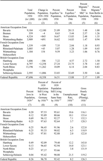
German expellees were very unevenly distributed across West German statesFootnote 9 (see Table 1). The regional distribution of expellees was initially determined by the spontaneous and largely undirected flight of Germans at the final stages of World War II (first phase of the displacement). As described, expellees initially fled to the most accessible regions west of the frontline and thus gathered in the eastern parts of the British and American zones (as well as in the Soviet zone). The wild expulsions (second phase) only added to the regional imbalances, as Germans were often driven just across the border into occupied Germany (for example, many Germans from the Sudetenland were forced into neighboring Bavaria). The organized expulsions (third phase) did little to level the regional imbalances in the distribution of expellees.
The plan to secure an equitable distribution of expellees across occupation zones fell to the French refusal to accept expellees into their occupation zone until 1947. France had not been invited to the Potsdam Conference and did thus not feel bound by the Treaty. Consequently, all expellees to West Germany were initially transferred to the American and British occupation zones. Moreover, many expellees did not reach their assigned zone. For instance, when the Czechoslovak expulsion trains crossed the U.S. zone, many of those bound for the Soviet zone jumped off (Douglas Reference Douglas2012, p. 190). And those who reached the Soviet zone were often determined to escape into the neighboring American and British zones.Footnote 10 Even in the American and British zones, organized expulsions did little to equalize the distribution of expellees. This was partly due to the collapse of German administration in 1945 and partly due to Allied policies. To prevent political unrest, the Allies instructed German authorities to house expellees, whenever possible, in private accommodations rather than refugee camps. Because cities were in shambles, most expellees were sent to the countryside (housing there had suffered less from bombing).Footnote 11 Yet, more rural states (Bavaria, Lower Saxony, and Schleswig-Holstein) were already overburdened with newcomers because of their proximity to the sending regions. As a result, the 1950 population share of expellees in the British zone ranged from 7.2 percent in the city state of Hamburg to 33 percent in Schleswig-Holstein (see Table 1, column 3).
Once expellees arrived in a region, their mobility was severely restricted. The Allies were anxious to control regional mobility and wanted all residents, not only expellees, to remain wherever they had been on the day of armistice. After the freeze was relaxed in 1947, moving required permits from the military administration. The permits were granted mostly to reunite families. General freedom of movement was only restored in May 1949 (Müller and Simon Reference Müller, Simon, Lemberg and Edding1959; Ziemer Reference Ziemer1973).
In addition to legal restrictions, moving was hampered by housing shortages and poor information about local labor market conditions. Indeed, the Allies initially banned almost all German newspapers, and the formation of expellee organizations. Consequently, the geographic distribution of expellee changed little before 1950. In fact, the correlation coefficient between the state-level expellee shares in 1946 and 1950 is 0.991 (see Table 1, columns 3 and 4). After 1950, however, large-scale resettlement programs were implemented and internal mobility picked up.
POPULATION CHANGES 1939–1950, OVERALL UNEMPLOYMENT AND WAGES IN WEST GERMAN STATES

Notes:
a Expellees are defined as German nationals or ethnic Germans who on 1 September 1939 lived (i) in the former German territories east to the Oder-Neisse line, (ii) the Saarland or, (iii) abroad, but only if their mother tongue was German. Figures for 1946 count all people who have lived abroad as expellees, as the census did not record their mother tongue. b Migrants from the SBZ and Berlin are defined as those residents of the 1950 population who had lived in the SBZ or in Berlin on 1 September 1939. c SBZ is the German abbreviation for the Soviet occupation zone (Sowjetische Besatzungszone). East Berlin is excluded. d The population share of Jews in Württemberg-Baden, Baden, and Württemberg-Hohenzollern are approximated by the share in Baden-Württemberg. The share for the Federal Republic includes the Saarland. e Ratio of a state's population in 1950 who on 1 September 1939 had lived in the same state and the state's population on 17 May 1939. f Children born after 1 September 1939 are assigned the place of residence of the father. g Ratio of the West German population in 1950 who on 1 September 1939 had lived in a given state and the state's population on 17 May 1939. h The unemployment rate is the share of unemployed among all employees. i The wage rate for Baden and Württemberg-Hohenzollern are approximated by the wage rate of Baden-Württemberg.
Sources:
Population figures are from the censuses of 13 September 1950, of 29 October 1946, and of 17 May 1939. Unemployment statistics are from the Federal Ministry of Labor and refer to 30 September 1950. Wage statistics are from the Federal Statistical Office. They refer to industrial workers and are from September 1950.
Population Change in West Germany, 1939 to 1950
The influx of almost eight million expellees was by far the most important driver of the dramatic increase in the West German population from 39.4 in 1939 to 47.7 million in 1950. But it was not the only one. The Census of 1950 also counted about one million people in West Germany who came from the Soviet zone (Sowjetische Besatzungszone, SBZ, excluding Berlin) (Table 1, column 5). In addition, half a million people, many of them evacuees, had lived in East or West Berlin (column 6). Overall, 3.3 percent of the West German population (excluding Berlin) had either lived in the SBZ or in Berlin before the war. The population share of migrants from the SBZ and Berlin was particularly large in Schleswig-Holstein (5.4 percent) and Lower Saxony (5.2 percent), two states with a border with East Germany. Therefore, the two states hosted both relatively more expellees and relatively more immigrants from East Germany than other states. In contrast, the share of migrants from the SBZ or Berlin was well below average in Bavaria, the state with the largest overall inflow of expellees.
West Germany experienced a large influx of immigrants, but it also suffered massive population losses between 1939 and 1950. First and foremost, millions of Germans died in World War II. In 1956 the Federal Statistical Office estimated that 1.8 million West German soldiersFootnote 12 and 180,000 West German civilians died in the war (Statistisches Bundesamt 1956a, 1956b). Second, almost none of the 103,300 Jews who had still lived in West Germany in May 1939Footnote 13 survived persecution and the Holocaust, and remained in West Germany after the war.Footnote 14 Third, 61,244 Germans were still held as prisoners of war or were detained abroad for criminal offenses in March 1950 (Statistisches Amt des Vereinigten Wirtschaftsgebietes 1950), although by then the vast majority of the approximately 11 million German prisoners of war had either been released or died in camps. Fourth, 89,900 West Germans, most of them relatives of U.S. or Canadian citizens, emigrated to North America and other overseas countries between 1945 and 1950 (Freund Reference Freund2004; Statistisches Bundesamt 1963).
In September 1950 only 38 million of the 47.7 million inhabitants of West Germany had already resided in West Germany before the war (or were born after 1939 to parents who had resided in West Germany in 1939). Without the population flows to West Germany, the West German population would have reached only 96.7 percent of its 1939 level (see Table 1, column 8). Population losses were particularly large in the two city states: Only 92.1 percent of Hamburg's and 93.9 percent of Bremen's population in 1939 still lived in (some state of) West Germany by 1950 (Table 1, column 8). In Hamburg alone, an estimated 40,000 people (or 2.3 percent of the 1939 population) died during the Allied air strikes. Hamburg was also home to an over-proportional number of Jews before the war (column 7), and both Bremen and Hamburg experienced greater emigration to North America than other regions.Footnote 15 In addition, the two city states also lost inhabitants to the other West German states. Many inhabitants of Bremen and Hamburg either fled or were evacuated from their home towns during the Allied air campaign. After the war ended, not all evacuees could return home, as housing was scarce and immigration restricted by law. Column 9 of Table 1 summarizes regional population losses in West Germany between 1939 and 1950. It reports the ratio of the number of individuals who resided in the same state both in 1939 and 1950 (or were born to them since 1939) to that state's population in 1939. The measure thus accounts for emigration, war-related deaths, and natural population movements. While the ratio is around 80 percent for Bremen and Hamburg, it exceeds 90 percent for all other West German states. More importantly, it does not correlate with expellee inflows once the two city states are excluded (correlation coefficient of 0.02).
Economic Conditions and Native-Expellee Relations
Expellees from East and Central Europe poured into a country whose infrastructure and housing stock had been heavily damaged during the war. However, despite the air raids, the aggregate capital stock of the German economy in 1950 was only 7 percent below its 1938 level. Massive investment into industrial capacity significantly increased productive capacity during the war and partially outweighed the impact of wartime destruction (Eichengreen and Ritschl Reference Eichengreen and Ritschl2009; Vonyó Reference Vonyó2012). Nevertheless, the inflow of expellees markedly decreased the capital-labor ratio of the West German economy.
While many native West Germans initially welcomed the expellees, relations between the two groups quickly deteriorated, when it became clear that the expellees were there to stay.Footnote 16 In June 1948 half of the expellees in the American Occupation Zone were dissatisfied by their treatment by native West Germans, up from 7 percent two years earlier (Merritt and Merritt Reference Merritt and Merritt1970). Conflicts between expellees and indigenous West Germans arose, in particular, over housing and employment. Natives were often unwilling to share their homes, and the enforced living together in a small space only created further tensions between native landlords and expellee tenants. Natives also saw the expellees as unwanted competitors in a tight labor market, and there is some evidence from local studies that employers discriminated against expellee workers (see, for example, Brosius Reference Brosius, Brosius and Hohenstein1985). To alleviate economic hardship, the states in the American and British occupation zones revived the unemployment insurance system of the Weimar Republic in 1947. The states in the French occupation zone followed suit in 1947/48. Unemployment benefits were paid for up to 26 weeks to persons (both natives and expellees) who had been employed for at least 26 weeks in the last 12 months (in a job that was subject to compulsory social insurance contributions). The level of benefits that a person received depended on her salary in the 13 weeks preceding her job loss. The replacement rate varied between 30 and 72 percent of the previous salary (Schmuhl Reference Schmuhl2003).
Economic recovery, in fact, came surprisingly quickly. In June 1948 a currency reform was implemented in the Western occupation zones and industrial production picked up rapidly. By 1950 industrial production almost doubled compared to 1948 and even surpassed prewar levels. Despite the boom in output, the currency reform led to a sharp increase in unemployment and, thus, aggravated the already tense relations between the native population and expellees (Connor Reference Connor2007).
By September 1950 regional unemployment rates differed markedly across states (see Table 1, column 10). At 21.5 percent, unemployment was highest in Schleswig-Holstein and well above the national average of 8.2 percent in Lower Saxony (14 percent) and Hamburg (12.2 percent). In contrast, it was quite low in Baden (2.6 percent) and Württemberg-Hohenzollern (2 percent). Despite these stark differences in unemployment rates, the quick resurrection of large industry-level unions that operated nationwide left little scope for regional wage differentiation, especially within industries (Eichengreen and Ritschl Reference Eichengreen and Ritschl2009; Vonyó Reference Vonyó2012).Footnote 17 While the average wages of industrial workers in the three states with the highest expellee inflows, Schleswig-Holstein, Lower Saxony, and Bavaria, were below the national average, regional wage differences were relatively small in comparison to the differences in unemployment rates (column 11). It seems that labor market adjustment to the very uneven influx of expellee workers mainly took place through employment, not wages.Footnote 18
EMPIRICAL STRATEGY
Defining Labor Market Segments
Following other studies of the labor market effects of immigration, we analyze the spatial correlation between labor market outcomes of natives and levels of immigration across local labor markets (German states). However, the overall fraction of expellees in a state is only an imperfect measure of competition between natives and migrants (Aydemir and Borjas Reference Aydemir and Borjas2011; Card Reference Card2001). To get a better measure, we split workers in each local labor market into skill groups. We then study the effect of an immigration-induced increase in the number of workers within a state-skill cell on the labor market outcomes of preexisting native workers in the same cell. We focus on labor market outcomes of males. Our definition of skill categories is based on occupations, as suggested by Card (Reference Card2001) and Rachel Friedberg (Reference Friedberg2001). We define occupations according to the eight categories (Berufsordnungen) in the first digit classification of occupations used by the German Federal Statistical Office for the Population Census 1950 (Systematik der Berufe 1950). The categories are: (I) Agricultural, forestry and fishery workers, gardeners, animal breeders, hunters; (II) Industrial occupations; (III) Craftsmen; (IV) Technical occupations; (V) Trade and transport occupations; (VI) Domestic and healthcare occupations; (VII) Administrative and legal occupations; (VIII) Education, research and arts occupations. Classifying workers into relatively broadly defined skill groups has the advantage that the resulting measure of immigrant competition does not miss competition from expellees in closely related occupations. Moreover, it reduces the possibility of endogenous selection into skill groups as workers are less likely to switch between more broadly defined occupations than between more narrowly defined occupations. However, some expellees were forced to switch even between broad occupational categories. They could simply not find jobs in occupations for which they were trained, and therefore often had to accept jobs for which they were overqualified (Connor Reference Connor2007).Footnote 19
Within state-occupation cells, expellees and natives were arguably close substitutes in the labor market. As noted above, expellees were not a selected subgroup of the sending region but represented a complete cross-section of society. They also shared the same language (though a different dialect) with natives.Footnote 20 Moreover, the ceded eastern territories, home to most expellees, had all been an integral part of Germany or Prussia for decades if not centuries.Footnote 21 Those expellees who had resided in the Sudetenland before World War II enjoyed wide-ranging minority rights in Czechoslovakia (Glassheim Reference Glassheim2000; Seton-Watson Reference Seton-Watson1938). Germans were guaranteed their own autonomous schools, proportional representation in parliament, and the right to use German in all official affairs. In fact, Germans and Czechs often lived in separate societies in Czechoslovakia, just as they had done in the Austro-Hungarian Empire. For instance, 97 percent of all German-speaking children attending primary school in Czechoslovakia went to a German school in 1935 (Seton-Watson Reference Seton-Watson1938).
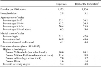
Table 2 compares sociodemographic characteristics of (male) expellees and the rest of the West German population in 1950. Expellees were slightly younger than non-expellees, as prewar birth rates had been somewhat higher in the former eastern territories than in the rest of Germany (Länderrat des Amerikanischen Besatzungsgebiets 1949). In addition, elderly expellees, in particular, might have died from the perils of the flight and expulsion. Being younger on average, expellees had a slightly higher probability of being single and tended to live in slightly smaller households. Overall, however, observed differences are small. The educational attainment of male expellees was slightly higher than that of native West Germans, but again differences were small (see Bauer, Braun, and Kvasnicka Reference Bauer, Braun and Kvasnicka2013 for further supportive evidence).
As noted earlier, agriculture was very important in the eastern territories. In 1939, 40.6 percent of the labor force was in agriculture in the eastern territories of pre-World War II Germany relative to an average of 25.9 percent (Länderrat des Amerikanischen Besatzungsgebiets 1949). This difference in the prewar occupational distribution of natives and expellees underlines the importance of stratifying local labor markets by occupation groups. As the agricultural sector was less productive than the non-agricultural sector (see, for example, Eichengreen and Ritschl Reference Eichengreen and Ritschl2009), the eastern territories were also relatively poor. Estimates suggest that the per capita national product in the eastern territories was around 20 percent below the German average (Gleitze Reference Gleitze1956).Footnote 22
SOCIODEMOGRAPHIC CHARACTERISTICS OF (MALE) EXPELLEES AND NATIVES IN WEST GERMANY, SEPTEMBER 1950

Notes:
Expellees are defined as German nationals or ethnic Germans who on 1 September 1939 lived (i) in the former German territories east to the Oder-Neisse line, (ii) the Saarland or (iii) abroad, but only if their mother tongue was German. The education statistics are for those who were born between 1885 and 1932 (aged 18 to 65 in 1950). The overwhelming majority of these persons should have completed their education by 1950.
1The education statistics distinguish between expellees and native West Germans. All other statistics distinguish between expellees and the rest of the population.
Sources:
All data except for educational attainment are from the census of 13 September 1950. Data on education is from a 10 percent sample of the census of 27 May 1970.
OLS Estimation
We are interested in the effects of immigration into a state-occupation cell on the employment rate of native males in the same cell. Let yij be the share of employed natives among all natives in occupation j who lived in state i in 1950. Our basic regression specification is
 \begin{equation}
y_{ij} = \alpha + \beta m_{ij} + x_i \gamma + d_j + \varepsilon _{ij}
\end{equation}
where mij is the share of male expellees in the total male labor force in state-occupation cell ij, xi a vector of state-specific control variables, dj a full set of occupation dummies, and ɛij the error term. In alternative specifications, we also add state dummies to equation 1 to account for unobservable factors at the state level. Our coefficient of interest, β, should be negative if expellee inflows reduced native employment.
The vector of state-specific control variables includes the share of housing units destroyed in the war, the prewar share of agricultural workers, and a dummy for the city states Bremen and Hamburg. The share of destroyed housing serves as a proxy for the war's economic dislocation.Footnote 23 It also captures the availability of housing, which influenced the regional distribution of expellees. The prewar share of workers employed in agriculture measures the importance of the agricultural base for a state. The most important receiving states Bavaria, Lower Saxony, and Schleswig-Holstein all had relatively large agricultural sectors. Finally, a dummy variable is assigned to the city- states of Hamburg and Bremen; they were both largely destroyed in the war and hosted relatively few expellees.Footnote 24 By including a set of occupation dummies, we control for occupation-specific productivity and demand factors. Such factors may have simultaneously affected occupational choices of natives and expellees and occupation-specific employment opportunities.
Errors are clustered at the skill-specific occupation-zone level to allow for correlation in economic shocks faced by individuals with similar skills who lived in the same occupation zone (American, English, or French). All regressions are weighted by the number of native male workers in each state-occupation cell.
IV Estimation
Our analysis uses cross-sectional data from 1950. By then, expellees might have already relocated to labor market segments with greater employment opportunities (restrictions on mobility had been fully phased out by 1949). This would lead to a spurious (positive) correlation between expellee shares and employment rates across labor market segments. More generally, if an unobserved factor increased both employment opportunities and the share of expellees in a state-occupation cell, we would underestimate the true employment effect of expellee inflows. To deal with unobserved factors at the stateFootnote 25 or state-occupation level, we instrument the expellee share in a state-occupation cell. Our instrumental variable strategy exploits regional variation in the prewar distribution of occupations as well as in the distance of the eastern territories and the Sudetenland to West German regions. Before proceeding, it is helpful to decompose the expellee share in a state-occupation cell as follows
 \begin{equation}
m_{ij} = \frac{{\sum\limits_s {\left({e_{si} \times occ_{sij}^e } \right)} }}{{\left({n_i \times occ_{ij}^n } \right) + \sum\limits_s {\left({e_{si} \times occ_{sij}^e } \right)} }}
\end{equation}
where esi is the total number of expellee workers from a sending region s that settled in the West German state i, ni is the native labor force in i, occe sij is the share of expellee workers from sending region s in state i and occupation j, and occn ij is the share of native workers in state i and occupation j. To illustrate the decomposition, let us consider the expellee share among agricultural workers in Schleswig-Holstein and suppose that there are just two sending regions, East Prussia and Silesia. Suppose further that Schleswig-Holstein took in 100,000 workers from East Prussia but only 10,000 workers from far-away Silesia; 20 percent of all expellees from the mainly rural state of East-Prussia but only 10 percent from more industrialized Silesia work as agricultural workers in Schleswig-Holstein. Finally, suppose that 10 percent of the 790,000 native workers in Schleswig-Holstein are agricultural workers. According to equation 2, the share of expellees among agricultural workers in Schleswig-Holstein is
 \begin{equation}
\frac{{100,000 \times 0.20 + 10,000 \times 0.10}}{{790,000 \times 0.10 + \left({100,000 \times 0.20 + 10,000 \times 0.10} \right)}} = 0.21
\end{equation}
Clearly, the share of expellees in a state-occupation cell depends both on the total inflow of expellees and on their occupational structure relative to that of the native population. Location and occupation choices are both potentially endogenous and may be affected by unobserved labor market conditions.
To construct our instrument, we proceed in two steps. First, we use geographical distances between sending and receiving regions to predict expellee flows from each sending to each receiving region. Second, we multiply the predicted flows by the prewar occupational structure of sending regions to obtain skill-specific expellee flows into West German states. Summing across sending regions gives the estimated migration-induced supply shock in occupation group j and state i. In what follows, we will describe the two steps in more detail. We start with the fact that the initial distribution of expellees across West German states in phase 1 (and to some extent in phase 2) of the displacement was largely driven by the distance between sending and receiving regions. For instance, Sudetenlanders mostly fled to neighboring Bavaria where they accounted for more than 50 percent of all expellees in 1946. In contrast, the share of Sudetenland expellees was negligible in faraway Schleswig-Holstein, the most northern state of West Germany. Conversely, Schleswig-Holstein was dominated by refugees from East-Prussia who arrived via the Baltic Sea. Such patterns of expellee inflows were driven by geography, and were arguably unrelated to local economic conditions in the receiving regions.
We run the following regression to predict the destinations of expellees
 \begin{equation}
share_{sr} = \delta + \lambda {\rm distance}_{sr} + \phi {\rm distance}_{sr}^2 + u_{sr}
\end{equation}
where sharesr is the share of male expellees from sending region s that resided in region r in 1950 and distancesi is a normalized measure of distance between sending and receiving regions.Footnote 26 Data on expellee shares are taken from the Census of 1950 (Statistisches Bundesamt 1953). We distinguish between ten source districts in the eastern territories and the SudetenlandFootnote 27 and 37 possible destination districts in West Germany (370 observations). Appendix Figure 1 maps the flows of expellees from the source districts to the destination districts. It shows that distance was important to the destination of expellee flows. An OLS regression of equation 3 demonstrates that distance between source and potential host regions reduced expellee inflows.Footnote 28 Coefficient estimates on the linear and quadratic distance terms are statistically significant at the 1 and 5 percent level, respectively, with an R2 of 0.225.Footnote 29 The prediction of sharesr is summed over all districts located in a state i and multiplied by the total number of expellees from sending region s to obtain an estimate for esi , the total inflow of expellee workers from sending region s into state i.
Unobserved labor market conditions in different labor market segments may not only affect location but also occupational choices of expellees within a state. The occupational distribution of sending regions in 1939 provides exogenous variation in the choice of occupations in 1950. The war insures that the occupational distribution of sending regions in 1939 is arguably exogenous to occupation-specific local labor market conditions in West German states in 1950. Many expellees came with occupation-specific human capital and they often sought employment in their former occupations after they arrived in West Germany.
The predicted skill-specific expellee inflow from a sending region s to a West German state i is the product of the predicted expellee inflow from s to i, êsi
, with the share of workers from s that worked in occupation j before the war, occsj
1939
. By summing over all sending regions, we obtain an estimate of the migration-induced supply shock in the relevant occupation group j and state i. The location of natives in specific segments of the labor market is potentially endogenous, too, as they may have responded to expellee inflows and moved to less crowded state-occupation cells. We address this problem by using the prewar population size of a state i, nativesi
1939
, and its occupational structure before the war, occij
1939
, to predict the postwar size of the native labor force in each state-occupation cell. The instrument for the share of expellees in state i and occupation
 $m\circ_y$
is then given by
 \begin{equation}
\hat m_{ij} = \frac{{\sum\limits_s {\left({\hat e_{si} \times occ_{sj}^{1939} } \right)} }}{{\left({native_i^{1939} \times occ_{ij}^{1939} } \right) + \sum\limits_s {\left({\hat e_{si} \times occ_{sj}^{1939} } \right)} }}
\end{equation}
DATA SOURCES AND DESCRIPTIVE STATISTICS
Employment, Expellees, and Covariates
Our main data source is the German population and occupation census of September 13, 1950.Footnote 30 It provides the size of the male labor force by state and occupation. The labor force comprises all economically active individuals (irrespective of their age), including the self-employed and unemployed. The census records current occupation for all individuals employed at the time of the enumeration and the last occupation for the unemployed. The census distinguishes between 440 occupations, which are aggregated to 38 occupation groups and nine occupation categories. Our analysis excludes workers in undefined occupations and helping family members, leaving us with 33 occupation groups and eight occupation categories. The census not only provides data on the total labor force in a state-occupation cell but also on the expellee labor force in the same cell, and thus allows us to calculate the share of expellees in each cell. The census defines expellees as German nationals or ethnic Germans who on 1 September 1939 lived (i) in the former German territories east to the Oder-Neisse line, (ii) the Saarland,Footnote 31 or (iii) abroad. The third group, however, includes only those Germans whose mother tongue was German (Statistisches Bundesamt 1953). Thus, by definition, all recorded expellees were German native speakers.
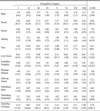
Appendix Table 1 reports the expellee share in each of the 88 state-occupation cells (11 states times eight one-digit occupations) that we use in our baseline regression. The expellee share varies widely across cells and ranges from 4.29 percent among agricultural, forestry, and fishery workers in Bremen to 35.10 percent among workers in industrial occupations in Schleswig-Holstein. Much of the variation in expellee shares is due to the very uneven distribution of expellees across states, as the very large state-level differences in the average expellee share show (last column of Appendix Table 1). Yet, expellees were also unevenly distributed across occupations. In the whole of West Germany, the share of expellees was highest in industrial occupations (18.03 percent) and lowest in technical occupations (11.51 percent). Perhaps surprisingly, the share of expellees among agricultural, forestry, and fishery workers (15.09 percent) was slightly below the average across all occupations. In fact, the proportion of expellees who worked in agriculture fell considerably between 1939 and 1950, and continued to fall in the years thereafter (Bauer, Braun, and Kvasnicka Reference Bauer, Braun and Kvasnicka2013; Lüttinger Reference Lüttinger1989). While many expellees initially began to work as manual laborers on farms, their productivity in agriculture was very low, and many of them were laid off after the currency reform in 1948 (Paqué Reference Paqué1987). Moreover, expellee farmers could rarely resume their business, as there was simply not enough farmland available for the newcomers (Connor Reference Connor2007). Some of them therefore left agriculture and sought jobs in more productive sectors.
Calculating the share of employed workers in the native labor force requires information on cell-specific unemployment of natives. Unfortunately, not all West German states published census data on occupation-specific unemployment. We thus resort to occupation-specific data on the registered unemployed provided by the Federal Ministry of Labor (Bundesministerium für Arbeit Reference für Arbeit1950). The classification of occupations is the same as the one used in the census. The unemployment data refer to 30 September 1950 (slightly after the labor force census). The unemployment data also use a slightly different definition of expellees than the census. It defines expellees as German nationals or ethnic Germans who on 1 January 1945 or before its flight or expulsion lived in the former German territories east to the Oder-Neisse line or abroad.
The census and the unemployment data only distinguish between expellees and the rest of the population. While the statistical agencies frequently refer to the rest of the population as natives (Einheimische) in their publications, these so-called natives are in effect non-expellees. Non-expellees include foreign civilians (but there were in effect none) and more importantly refugees from the Soviet zone and Berlin. The average employment rate is therefore a weighted average of the employment rate of natives and of migrants from the SBZ and Berlin. However, migrants from the SBZ accounted for only 2.6 percent of non-expellees, and migrants from Berlin for another 1.3 percent. The weight put on the employment rate of migrants from the SBZ and Berlin is therefore small.Footnote 32 Moreover, the labor market performance of workers from the Soviet Occupation Zone was comparable to the performance of the indigenous West German population (Lüttinger Reference Lüttinger1989). Therefore, the employment rate of non-expellees should be a very good proxy for the employment rate of natives. For simplicity, we continue to refer to non-expellees as natives.
The share of destroyed housing units in a state comes from Deutscher Städtetag (Reference Städtetag1949). The prewar share of workers employed in agriculture is based on the population and occupation census of 17 May 1939 (Statistisches Bundesamt 1954).Footnote 33
Instrument
The prewar distribution of occupations is taken from the occupation census of 17 May 1939 (Statistisches Reichsamt 1941). The one- and two-digit classification of occupations used in 1939 does not exactly match with the classification used in 1950. In the absence of an official recoding scheme, we use the finer three-digit classification of occupations of 1939 and assign, whenever possible, each occupation to the corresponding one- and two-digit occupation defined in the Census of 1950. The 1939 Census provides three-digit occupation data for 27 administrative units. Among those units are the five most important former homelands of expellees, namely East Prussia, Silesia, West Prussia, Pomerania, and the Sudetenland. When the 1939 administrative units do not match the later West German states, we calculate the prewar occupational structure of a later West German state as the population-weighted average of the administrative units on whose territories the state was founded.
Based on the predicted expellee inflows from source to receiving areas and the prewar distribution of occupations, we then calculate the instrument for the share of expellees in state-occupation cells.Footnote 34 Actual and predicted expellee inflows are highly correlated. An OLS regression of actual on predicted expellee inflows yields a precisely estimated coefficient of 0.504, with an R2 of 0.353.
RESULTS
Main Results
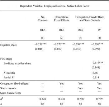
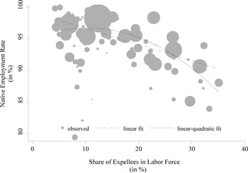
Table 3 summarizes our main results on the relationship between expellee inflows and employment opportunities of natives. Column 1 presents estimates from the most parsimonious OLS model that includes the share of expellees in the total male labor force as the only regressor. The highly significant coefficient estimate of −0.256 indicates that a 10 percentage point increase in the share of German expellees in a state-occupation cell is associated with a reduction of the native employment rate in the same cell by 2.6 percentage points. The dashed line in Figure 2 draws the linear regression line on the scatter plot of native employment rates and expellee shares and shows that the negative effect of expellee inflows is not driven by outliers.
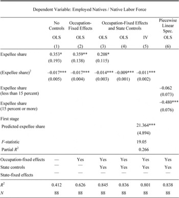
As a next step, we add controls at the occupation and state level to account for potential confounding factors. First, we include a full set of occupation dummies (column 2). The inclusion of occupation dummies eliminates national occupation-specific demand and productivity factors. Second, we add the prewar share of workers employed in agriculture, the share of destroyed housing units and a dummy for the city-states of Hamburg and Berlin to the model (column 3). These factors, all measured at the state level, influenced expellee flows and may potentially be related to employment outcomes of local residents. After the inclusion of these control variables, however, the coefficient on the expellee share changes little and remains highly statistically significant.
To address the concern that unobserved factors render the expellee share in state-occupation cells endogenous, we instrument the actual by the predicted expellee share (while still controlling for occupation-fixed effects and state controls). The results are presented in column 4 of Table 3. The first-stage regression shows that the predicted prevalence of expellees in a state-occupation cell is strongly and significantly correlated with the actual prevalence and explains large parts of its variation. The F-statistic is high, suggesting that we do not have a weak instrument problem. The IV estimation confirms that expellee inflows had an important impact on employment opportunities of natives. The IV estimate is somewhat larger than the corresponding OLS estimate. We now find that a 10 percentage point increase in the expellee share decreased the share of employed in the native labor force by 4 percentage points. This specification is our preferred one, as it accounts for the potential endogeneity of expellee shares in state-occupation cells.
EXPELLEE INFLOWS AND NATIVE EMPLOYMENT, LINEAR SPECIFICATION

*** = Significant at the 1 percent level.
Notes:
Standard errors are in parentheses and clustered at the skill-occupation-zone level. All regressions are weighted by the native male labor force in each state-occupation cell.
EXPELLEE INFLOWS AND NATIVE EMPLOYMENT

A remaining concern is the (positive) correlation between the inflow of expellees and the inflow of migrants from the SBZ and Berlin. If migrants from the SBZ and Berlin also had a negative effect on native employment, we will overestimate the effect of expellees on native employment. This omitted variable bias is unlikely to vanish in the IV estimation, as distance from West Germany to the eastern territories is correlated with the distance to East Germany. Unfortunately, we cannot directly control for the share of migrants from the SBZ and Berlin in a state-occupation cell, as the census does not provide data on the occupation of migrants from the SBZ and Berlin. Instead, we assess the potential magnitude of the bias, using the standard omitted variable bias formula. The bias will be larger, (i) the greater the effect of East Germans on native employment is and (ii) the stronger the correlation between the share of expellees and of East Germans across state-occupation cells. If we assume that migrants from East Germany had the same effect on native employment than expellees, and that the occupational distribution of the two groups were identical,Footnote 35 we find that our estimated effect exceeds the true effect by at most 17.8 percent (see the Appendix for details).
The size of expellee inflows differed dramatically across West Germany. To allow for potential nonlinearities in the relation between the native employment rate and the share of expellees, we add the squared expellee share as an additional regressor. Column 1 of Table 4 presents the corresponding regression results. Both the linear and quadratic expellee share terms are statistically significantly different from zero. The linear-quadratic regression specification fits the data much better than the linear specification. The R2 rises from 0.328 to 0.412 after the inclusion of the squared expellee share. Adding occupation dummies and state controls reduces the magnitude of the (positive) coefficient estimate on the linear expellee share term but hardly changes the coefficient estimate on the quadratic term (column 3). The solid line in Figure 3 plots the linear-quadratic regression from column 1 of Table 4. It shows that, the relation between the native employment rate and the share of expellees is almost flat until the expellee share exceeds a level of roughly 15 percent.
Once this level was reached, however, additional expellee inflows had an increasingly negative impact on native employment. Columns 4 and 5 present OLS and IV estimates of a specification that includes the squared but not the linear expellee share term as regressor. Estimating the linear-quadratic specification using the IV approach would require a second instrument, which we do not have. The IV regression for the nonlinear case thus focuses on a specification with a quadratic expellee share term only. Column 4 shows that the fit of the OLS regression is hardly reduced by dropping the linear expellee share term (the R2 drops from 0.845 to 0.836). The IV estimate of the squared expellee share is highly statistically significant and slightly larger than the OLS estimate. We also consider a piecewise linear specification to investigate the nonlinearity of the displacement effect (column 6). In particular, we allow the effect of expellee inflows on native employment to differ for labor market segments with relatively low expellee shares of less than 15 percent and labor market segments with relatively high expellee shares of 15 percent or more. Again, we find that the displacement effect is limited to labor market segments with high expellee inflows. While the coefficient is close to zero and not significant in labor market segments with relatively low expellee inflows, it becomes highly negative (coefficient estimate of −0.48) in labor market segments with high expellee inflows.
EXPELLEE INFLOWS AND NATIVE EMPLOYMENT, (LINEAR-)QUADRATIC SPECIFICATION

* = Significant at the 10 percent level.
** = Significant at the 5 percent level.
*** = Significant at the 1 percent level.
Notes:
Standard errors are in parentheses and clustered at the skill-occupation-zone level. All regressions are weighted by the native male labor force in each state-occupation cell.
Estimation with State-Fixed Effects
Predicted expellee inflows are only a valid instrument for actual expellee inflows if they are uncorrelated with unobserved labor market conditions in a state-occupation cell. One may be concerned that the distance from the former eastern territories to West German states, which we use to predict expellee inflows, correlates with unobserved state characteristics that directly affected native employment rates. If so, the exclusion restriction of our distance-based instrument will fail. Adding state-fixed effects removes all (observed and unobserved) heterogeneity between states, so that any remaining unobserved labor market conditions are specific to a state-occupation cell. The IV estimation then relies only on regional variation in the prewar occupational structure of expellees relative to natives to identify the employment effect of immigration.
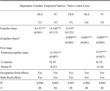
Table 5 shows the results of re-estimating the linear, linear-quadratic and quadratic specifications with both occupation and state dummies. In all specifications, expellee inflows coefficients remain negative and highly statistically significant. Adding fixed effects to the OLS regressions does, however, reduce the magnitude of the negative employment effect. The linear OLS regression now suggests that, on average, a 10 percentage point increase in the share of German expellees decreased the employment rate of natives by 1.5 percentage points (column 1). The smaller magnitude of the coefficient may indicate that our vector of control variables misses important state characteristics that simultaneously increased the inflow of expellees and reduced native employment. It may, however, also reflect the fact that state-fixed effects take away most of the variation in the data and potentially intensify problems related to measurement error (biasing our estimates towards zero).
Once we instrument actual with predicted expellee inflows, the results of the fixed effects regressions are very similar to those of our baseline regressions. The linear IV regression with fixed effects suggests that a 10 percentage point increase in the share of German expellees decreased the employment rate of natives by 3.3 percentage points (column 2). This is very close to our preferred point estimate of 4 percentage points from the linear IV regression without fixed effects (Table 3, column 4). We also continue to find strong evidence for a nonlinear relation between native employment and expellee shares in the fixed effects regressions (Table 4, columns 3–5).
EXPELLEE INFLOWS AND NATIVE EMPLOYMENT, FIXED EFFECTS REGRESSIONS

* = Significant at the 10 percent level.
*** = Significant at the 1 percent level.
Notes:
Standard errors are in parentheses and clustered at the skill-occupation-zone level. All regressions are weighted by the native male labor force in each state-occupation cell and include a full set of occupation and state dummies.
Displacement Effect over Time
In 1950, the year of our analysis, unemployment in West Germany reached its postwar peak. As West German economic growth soared in the 1950s, however, unemployment fell quickly and was virtually nonexistent by 1960.Footnote 36 In fact, expellees soon provided an important labor reservoir for the booming postwar industry and thus arguably made an important contribution to West Germany's economic miracle (Wirtschaftswunder) (Ambrosius Reference Ambrosius1996). Therefore, we expect the negative employment effect of the expellee influx to have been only short-lived.
EXPELLEE INFLOWS AND OVERALL EMPLOYMENT IN 1950 AND 1953

*** = Significant at the 1 percent level.
Notes:
Standard errors are in parentheses and clustered at the skill-occupation-zone level. All regressions are weighted by the size of the male labor force in each state-occupation cell in the respective year.
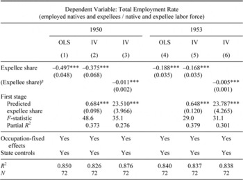
To test this prediction, we reestimate our main regressions using the employment rate of all males (including both natives and expellees) in 1950 and 1953 as new dependent variables (and the same set of explanatory variables as before). We expect that the negative employment effect of the expellee inflows was already markedly smaller in 1953 than in 1950. Unfortunately, data on employment rates by state and occupation are no longer available after 1953, and the statistic for 1953 does not distinguish between natives and expellees (so that we cannot calculate the cell-specific employment rate of natives in 1953).
The results in Table 6 show that the negative employment effect of the expellee inflows on the overall employment rate was already much smaller in 1953 than in 1950. According to the results of the linear IV specification, a 10 percentage point increase in the share of expellees reduced the overall employment rate by 1.7 percentage points in 1953 (column 5), compared to 3.8 percentage points in 1950 (column 2).Footnote 37 Given that full employment was reached by 1960, one can reasonably assert that the inflow of expellees did not significantly reduce employment rates in the long run.
CONCLUSION
We study the employment effects of one of the largest forced population movements in human history, the massive influx of German expellees from Eastern Europe to West Germany after World War II. We find that a 10 percentage point increase in the share of expellees in the labor force decreased the employment rate of natives by 4 percentage points. The displacement effect was, however, relatively short-lived and declined rapidly over time. Still, we find a substantially larger short-run displacement effect of immigration than most contemporary studies.
This difference might be due to the sheer size of the expellee inflows. In fact, the strong average displacement effect of expellee inflows is exclusively driven by labor market segments that experienced very high inflow rates (15 percent or more). The nonlinear relation between expellee inflows and native employment fits well with the widely shared belief that postwar West Germany, which was devastated by the Allied bombing campaigns, suffered from a relative shortage of physical capital (Giersch Reference Giersch1993; Paqué Reference Paqué1987). The scope to substitute labor for capital was limited, so the argument goes, and the maximum level of employment in labor market segments was restricted by capacity constraints.Footnote 38 As a result, labor market segments could initially only accommodate a limited inflow of expellees. The uneven expellee inflows apparently exhausted the capacity constraints in some labor market segments but not in others, and led to marked differences in local unemployment rates.
Our findings suggest that, up to a saturation point, the West German labor market was able to absorb expellees without adverse labor market effects. Given that native workers had to compete with highly comparable expellees who were forced to migrate to West Germany despite the dire labor market prospects, this result is remarkable. It may suggest that under today's much more favorable circumstances modest levels of immigration may have no or only small effects on native employment—as much of the contemporary literature indeed suggests (see Kerr and Kerr Reference Kerr and Kerr2011 for a summary of the literature and Longhi, Nijikamp, and Poot Reference Longhi, Nijkamp and Poot2010a, Reference Longhi, Nijkamp and Poot2010b for meta-analyses). Clearly, the levels of immigration witnessed by Germany at the end of World War II are rarely reached by today's immigration flows.
More generally, our finding of a nonlinear effect of immigration on native employment reminds us of the simple fact that the structural relationship between labor supply shifts and wages or employment is unlikely to be constant as we move along the labor demand curve. If the displacement effect of immigration increases with the size of the inflow (as it does in our setting), an equal distribution of immigrants across labor market cells can help to reduce the average displacement effect—and thus reduce the burden borne by natives on the labor market.
Appendix
Appendix 1: Additional Figures and Tables
DISTRICT-TO-DISTRICT FLOWS OF EXPELLEES FROM THE EASTERN TERRITORIES AND THE SUDETENLAND TO WEST GERMANY

EXPELLEE SHARES IN STATE-OCCUPATION CELLS (male population)

Appendix 2: Deriving the Bias from Omitting Migrants from the SBZ and Berlin
To derive the bias from omitting migrants from the SBZ and Berlin from our regression, start with our basic (unconditional) regression equation
 \begin{equation}
y_{ij} = \alpha + \beta m_{ij} + \varepsilon _{ij}
\end{equation}
Now suppose that the true regression equation contains the share of migrants from the SBZ and Berlin, denoted m* ij
 \begin{equation}
y_{ij} = \alpha ' + \beta 'm_{ij} + \xi m_{ij}^* + u_{ij}
\end{equation}
Suppose further that the share of migrants from the SBZ and Berlin in a state-occupation cell is related to the share of expellees in the same cell as follows
 \begin{equation}
m_{ij}^* = \theta + \vartheta m_{ij} + \upsilon _{ij}
\end{equation}
where θ is a constant and υ is an error term. Plugging (A3) into (A2) and rearranging gives
 \begin{equation}
y_{ij} = \left({\alpha ' + \xi \theta } \right) + \left({\beta ' + \vartheta \xi } \right)m_{ij} + \left({\xi \upsilon _{ij} + u_{ij} } \right)
\end{equation}
Therefore, the estimated effect of expellee inflows on native employment, β, equals the true effect, β’, plus a bias ϑ ξ
 \begin{equation}
\beta = \beta ' + \vartheta \xi
\end{equation}
The bias ϑ ξ depends i) on the strength of the effect of the inflow of migrants from the SBZ and Berlin on native employment (as captured by ξ) and ii) on the strength of the association between mij and m* ij (as captured by ϑ). If the inflow of migrants from the SBZ and Berlin has identical employment effects than the inflow of expellees (in other words, if ξ = β’), we can rewrite (A5) as β/β’ = 1 + ϑ.Footnote 39 The estimated coefficient β therefore exceeds β’ by ϑ percent.
To obtain an estimate of ϑ, we have to make some assumption on the occupational structure of migrants from the SBZ and Berlin (in West Germany in 1950). As we want to establish an upper bound on the omitted variable bias, we assume that the occupational distribution of migrants from the SBZ and Berlin is identical to that of expellees (so that the correlation between mij and m* ij is maximized). We then approximate the share of migrants from the SBZ and Berlin in a state-occupation cell as follows
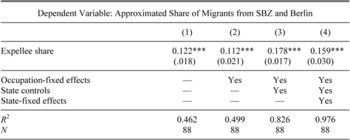
THE RELATION BETWEEN THE SHARE OF MIGRANTS FROM SBZ/BERLIN AND OF EXPELLEES

 \begin{equation}
m_{ij}^* = \frac{{pop_i^{SBZ/Berlin} }}{{pop_i^{Expellees} }} \times m_{ij}
\end{equation}
where popi SBZ/Berlin is the male population of state i who on 1 September 1939 had lived in the SBZ or Berlin, and popi Expellees is the male population who had lived in the eastern territories or abroad. The approximated share of migrants from the SBZ or Berlin in a state-occupation cell equals the share of expellees in the same cell times the state-level ratio of migrants from the SBZ and Berlin to expellees. We then regress m* ij on mij (and controls) to obtain an estimate of ϑ. The results suggest that an increase of the expellee share by 1 percentage point is associated with an increase of the share of migrants from the SBZ and Berlin by between 0.112 and 0.178 percentage points (see Appendix Table 2). These estimates correspond to the deviation of β from β’ (if ξ indeed equals β’).