2. Parameter regime

For the parameters explored in this study, we focus on the ‘Farfield’ observations of the internal tide that propagated south-west of the Hawaiian Islands (Rainville & Pinkel Reference Rainville and Pinkel2006). These observations, taken over 40 days in the autumn of 2001, were made $430$ km south-west of Oahu at a latitude of 18.39$^\circ$N. The Coriolis parameter at that latitude was $0.0000459\ \mbox {s}^{-1}$, in which here, and throughout this paper, we write $\mbox {s}^{-1}$ to represent radians per second. The ocean depth at the Farfield location was $H\simeq 5200$ m.

Measurements of temperature and conductivity (salinity) taken between the surface and $800$ m depth showed that the background density profile decreased approximately exponentially with depth below a $100$ m deep surface mixed layer. In particular, the buoyancy frequencies at $100$ m and $800$ m depth were approximately $10$ and $2$ cycles per hour (c.p.h.), respectively. From these data, we estimate the background squared buoyancy frequency profile below $z_0=-100$ m to be $N^2(z) \simeq N_0^2\,{\rm e}^{(z-z_0)/d}$, with $N_0\simeq 0.017\ \mbox {s}^{-1}$ ($\simeq 9.7$ c.p.h.) and $d\simeq 218$ m.

From measurements of both the isopycnal displacements and baroclinic energy flux, the dominant disturbances to the background took the form of vertical mode-1 internal tides at the semi-diurnal frequency of the lunar ($M_2$) tide, $\omega \simeq 0.000141\ \mbox {s}^{-1}$. Satellite altimetry and numerical modelling determined the horizontal wavelength of the $M_2$ internal tide to be approximately $150$ km (Rainville et al. Reference Rainville, Johnston, Carter, Merrifield, Pinkel, Worcester and Dushaw2010). The corresponding horizontal wavenumber is $k\simeq 4.2\times 10^{-5}\ \mbox {m}^{-1}$.

The root-mean-square isopycnal displacements of the semi-diurnal tide was largest between $400$ and $700$ m depth, with values $\gtrsim 25$ m at the spring tides, and $\lesssim 5$ m at the neap tides (Rainville & Pinkel Reference Rainville and Pinkel2006). From this we estimate the half peak-to-peak displacement to be $A_0\simeq 15\ (\pm 10)$ m.

We use these data to cast the key variables of our study as non-dimensional parameters that will guide approximations used in the following theory section as well as setting variables used in numerical simulations. The e-folding depth of the stratification relative to the ocean depth is $d/H \simeq 0.04$. The relative Coriolis and internal tide frequencies are $f/N_0\simeq 0.003$ and $\omega /N_0\simeq 0.008$, respectively. The relative horizontal wavenumber is $kH \simeq 0.2$. The half peak-to-peak amplitude relative to the ocean depth is $A_0/H \simeq 0.003\ (\pm 0.002)$. Taken relative to the e-folding depth of the stratification, we have $\alpha \equiv A_0/d \simeq 0.075 (\pm 0.050)$.

We are particularly interested in the behaviour of the internal tide as it travels south towards the equator, where ${f=0}$. Thus we neglect variations in bottom depth and assume that $kH\simeq 0.2$ is fixed. For simplicity, the equations are solved on the $f$-plane, with the evolution of the internal tide examined separately at different fixed values of $f$ between $0.003N_0$ and $0$.

3. Theory

Here, we present the theory for superharmonic excitation induced by a horizontally propagating, vertical mode-1 internal wave. After presenting the equations of motion, the vertical structure equation and polarization relations for small-amplitude internal waves are presented. Evolution equations are then derived for superharmonics excited by triad interactions between internal modes. In this work, we ignore the self-interaction of waves leading to an induced Eulerian flow (Bühler Reference Bühler2014; van den Bremer, Yassin & Sutherland Reference van den Bremer, Yassin and Sutherland2019). This is because, as is shown in our companion paper (Sutherland & Yassin Reference Sutherland and Yassin2022), superharmonics are near-resonant with the parent wave, whereas the induced Eulerian flow is not. Hence this flow has negligible influence upon the parent wave and its superharmonics.

3.1. Equations of motion

We consider the motion of inviscid, non-diffusive, incompressible Boussinesq fluid on the $f$-plane in a horizontally periodic channel bounded above and below by free-slip boundary conditions. The waves in this domain are taken to be two-dimensional, having structure in the along-wave ($x$) and vertical ($z$) directions. Although there can be motion in the spanwise ($y$) direction, the fields of interest are independent of $y$.

The momentum equations are

(3.1a–c)\begin{equation} \frac{{\rm D}u}{{\rm D}t} -fv ={-}\frac{1}{\rho_0}\, \frac{\partial p}{\partial x},\quad \frac{{\rm D}v}{{\rm D}t} +fu = 0,\quad \frac{{\rm D}w}{{\rm D}t} ={-}\frac{1}{\rho_0}\, \frac{\partial p}{\partial z} + b,\end{equation}

in which ${\rm D}/{\rm D}t\equiv \partial _t + u\partial _x + w\partial _z$ is the material derivative, $u$, $v$ and $w$ are the components of velocity in the $x$, $y$ and $z$ directions, respectively, $b=-g\rho /\rho _0$ is the buoyancy, $p$ and $\rho$ are the pressure and density fluctuations, respectively, and $\rho _0$ is the characteristic density. In these expressions, gravity ($g$) and the Coriolis parameter ($f$) are assumed to be constant. From internal energy conservation, we have

(3.2)\begin{equation} \frac{{\rm D}b}{{\rm D}t} ={-}N^2 w,\end{equation}

in which $N^2(z) = -(g/\rho _0) \, {\rm d} \bar {\rho }/{\rm d} z$ is the squared buoyancy frequency, and $\bar {\rho }(z)$ is the background density. In a uniformly stratified fluid, $\bar {\rho }$ increases linearly with depth and $N^2$ is constant. In this study, $N^2$ is taken to be $z$-dependent, as is necessary for the excitation of superharmonics.

By assuming that the fluid is incompressible, the $x$- and $z$-velocity components can be written in terms of the streamfunction $\psi$:

(3.3a,b)\begin{equation} u ={-}\frac{\partial\psi}{\partial z}, \quad w = \frac{\partial\psi}{\partial x}.\end{equation}

Taking the curl of the $x$- and $z$-momentum equations gives an equation for the evolution of the spanwise vorticity, $\zeta \equiv \partial _z u - \partial _x w$:

(3.4)\begin{equation} \frac{{\rm D}\zeta}{{\rm D}t} ={-}\frac{\partial b}{\partial x} + f\,\frac{\partial v}{\partial z}.\end{equation}

These nonlinear equations can be manipulated to be written as a linear operator acting on the streamfunction $\psi$, being forced by nonlinear terms (Wunsch Reference Wunsch2017; Baker & Sutherland Reference Baker and Sutherland2020):

(3.5)\begin{equation} \mathcal{L}\psi = \boldsymbol{\nabla}\boldsymbol{\cdot}\boldsymbol{F},\end{equation}

in which

(3.6)\begin{equation} \mathcal{L} \equiv\partial_{tt}\nabla^2 + N^2 \partial_{xx} + f^2 \partial_{zz}\end{equation}

and

(3.7)\begin{equation} \boldsymbol{F} \equiv\partial_t(\boldsymbol{u}\zeta) - \partial_x (\boldsymbol{u}b) + f\,\partial_z(\boldsymbol{u}v).\end{equation}

Here, $\nabla ^2 = \partial _{xx}+\partial _{zz}$ is the Laplacian, and $t$, $x$ and $z$ subscripts denote the corresponding partial derivatives. In solving the above equations, the domain is taken to be bounded above and below by free-slip horizontal boundaries at $z=0$ and $z=-H$.

3.2. Small-amplitude waves

Laying the groundwork for the nonlinear studies that follow, here we describe the initial structure of the internal tide, which we refer to hereafter as the ‘parent wave’, and then generalize this to describe the structure and polarization relations associated with the parent wave and its superharmonics.

The parent wave has a prescribed horizontal wavenumber $k$, and vertical displacement amplitude $A_0$. Although in reality the internal tide is modulated spatially, it is unnecessary to include these dynamics in the consideration of superharmonic excitation. The streamfunction characterizing the parent wave is given by

(3.8)\begin{equation} \psi^{(1)} = \frac{1}{2}\,\frac{\omega d}{k}\,\alpha\,a_1(T)\,\hat{\psi}_1(z) \, {\rm e}^{\mathrm{i}(kx- \omega t)} + \text{c.c.},\end{equation}

in which $\text {c.c.}$ denotes the complex conjugate, and $a_1(T)$ represents the slow time ($T$) evolution of amplitude, to be discussed in detail below. Somewhat arbitrarily, we have introduced $d$ to be the characteristic vertical scale of variation of $N^2(z)$, so that $\alpha \equiv A_0/d$ is the non-dimensional initial amplitude of the parent wave, expressed as the maximum vertical displacement relative to $d$. Substituting (3.8) into $\mathcal {L}\psi ^{(1)} =0$ gives an eigenvalue problem for the vertical structure $\hat {\psi }_1$ and its associated frequency $\omega$:

(3.9)\begin{equation} \hat{\psi}_1^{\prime\prime} + k^2\,\frac{N^2-\omega^2}{\omega^2-f^2}\,\hat{\psi}_1 =0, \quad \hat{\psi}_1({-}H)=\hat{\psi}_1(0)=0.\end{equation}

As justified below (see also Baker & Sutherland Reference Baker and Sutherland2020), we consider only superharmonics having the vertical structure of mode-1 waves for which $\hat {\psi }_1(z)>0$ for $-H< z<0$. These eigenfunctions are normalized so that $\max \{\hat {\psi }_1\}=1$. The vertical structure is plotted in figure 1 as computed for waves in exponential stratification,

(3.10)\begin{equation} N^2(z) = N_0^2\,{\rm e}^{(z-z_0)/d} \quad\text{for }{-H}\leq z\leq 0,\end{equation}

and in exponential stratification that includes a surface mixed layer

(3.11)\begin{equation} N^2(z) = \left\{\begin{array}{@{}ll} 0 & z_0< z\leq 0, \\ N_0^2\,{\rm e}^{(z-z_0)/d} & -H\leq z\leq z_0. \end{array}\right. \end{equation}

In both cases, we set $d=0.04H$ and $z_0=-0.019H$, equivalent to a 100 m deep mixed layer in an ocean of depth $H=5200$ m. These plots demonstrate that the vertical structure is not particularly sensitive to the presence of a mixed layer. The peak in the vertical structure occurs at depth $-0.14H$ (approximately $700$ m depth), which is comparable to the maximum isopycnal displacements observed at the Farfield site south-west of Hawaii (Rainville & Pinkel Reference Rainville and Pinkel2006).

Figure 1.

(a) Profiles of exponential stratification with $d=0.04H$ and $N=N_0$ at $z_0=-0.019H$ (thick black line) and of the same exponential stratification but with $N=0$ above $z=-0.019H$ (red line). (b) The corresponding vertical structure functions of mode-1 waves. The structure was computed for $k=0.2H$ and $f=0.003N_0$. In both cases, only the top 30 % of the full domain height is plotted.

The evolution of the parent wave is given by $a_1(T)$, in which $T=\epsilon t$ describes the slow time variation ($\epsilon \ll 1$) of the parent wave due to interactions with the superharmonics that it excites. With the streamfunction defined by (3.8), the initial non-dimensional amplitude of the parent wave is $a_1(0)=1$. As in Baker & Sutherland (Reference Baker and Sutherland2020), we will show that the small parameter $\epsilon$ is determined by the degree to which the forcing of the $2k$-superharmonic by the parent wave at frequency $2\omega$ is off-resonant with the natural frequency $\omega _2$ of the mode-1 superharmonic.

The parent wave self-interacts through the nonlinear terms in (3.7) to excite a superharmonic with wavenumber $2k$. The parent wave and its $2k$-superharmonic can then interact creating higher superharmonics, modifying the amplitude of the parent wave and superharmonics in time.

For convenience, we write the streamfunction for each of the parent ($n=1$) and its superharmonics ($n=2,3,\ldots$) as

(3.12)\begin{equation} \psi^{(n)}= \frac{1}{2}\,\alpha\,\frac{\omega d}{k}\,\psi_n \, {\rm e}^{\mathrm{i} n(kx-\omega t)} + \text{c.c.},\end{equation}

in which

(3.13)\begin{equation} \psi_n = a_n(T)\,\hat{\psi}_n(z), \quad n=1,2,3,\ldots.\end{equation}

The vertical structure is given by the solution to the eigenvalue problem

(3.14a,b)\begin{equation} \hat{\psi}_n^{\prime\prime} + (nk)^2\,\frac{N^2-\omega_n^2}{\omega_n^2-f^2}\,\hat{\psi}_n =0,\quad \hat{\psi}_n({-}H)=\hat{\psi}_n(0)=0,\quad n=1,2,3,\ldots,\end{equation}

in which $\omega _n$ is the natural frequency of a vertical mode-1 wave having wavenumber $nk$. As in (3.8), the amplitude $a_n(T)$ of the waves is assumed to depend upon a slow time scale $T=\epsilon t$.

The expression for $\psi ^{(n)}$ supposes that the frequency of the wave with wavenumber $nk$ is $n\omega$. This assumption is made because integer multiples of the parent wave frequency result from wave–wave interactions in the nonlinear terms. However, for $n>1$, the frequency $n\omega$ is not equal to the natural frequency $\omega _n$ of the mode-1 wave with wavenumber $nk$, although the difference in frequencies may be close, as demonstrated in the next subsection. It is this slight mismatch that leads to off-resonant forcing of successive superharmonics.

Given the streamfunction of the parent wave and its superharmonics, the other fields appearing in the nonlinear terms of $\boldsymbol {F}$ in (3.7) can be found from the polarization relations. These expressions are listed in table 1.

Table 1.

Expressions for the polarization relations of the fields with horizontal wavenumber $nk$, $n=1,2,\ldots$. The actual fields are found by multiplying by $\alpha (\omega d/k)\,\exp [\mathrm {i}n(kx-\omega t)]/2$ and adding the complex conjugate. In these expressions, primes on $\hat {\psi }_n$ denote $z$-derivatives.

3.3. Superharmonic cascade

Now consider the triad interaction in which a wave having wavenumber $lk$ interacts with a wave having wavenumber $mk$ to force a disturbance with wavenumber $nk$, in which $n=l+m$. Here, $l$, $m$ and $n$ can be negative as well as positive integers, with negative numbers arising from the complex conjugate terms in the polarization relations. From (3.7), the nonlinear forcing of $nk$-waves by $mk$- and $lk$-waves is given by

(3.15)\begin{equation} \boldsymbol{\nabla}\boldsymbol{\cdot}\boldsymbol{F}_{ml} = \boldsymbol{\nabla}\boldsymbol{\cdot}[\partial_t(\boldsymbol{u}_m\zeta_l) - \partial_x(\boldsymbol{u}_m b_l) + f\,\partial_z(\boldsymbol{u}_mv_l)], \quad |m|,|l|\geq 1,\end{equation}

in which $n=m+l$.

To find the response to the forcing, we use (3.6) to expand ${\mathcal {L}}\psi ^{(n)}$, with time derivatives acting upon $a_n(T)$ as well as the complex exponential. However, assuming that $\epsilon$ is small, the term $\epsilon ^2\,{\rm d}^2a_n/{\rm d}T^2$ can be neglected. Thus we find, for $n=1,2,3,\ldots$,

(3.16)\begin{equation} {\mathcal{L}}\psi^{(n)} \simeq \frac{1}{2}\,\alpha\,\frac{\omega d}{k}\, (nk)^2\,\frac{N^2-f^2}{\omega_n^2-f^2} \left[2\mathrm{i} n\omega \epsilon\,\frac{{\rm d}a_n}{{\rm d}T} + [(n\omega)^2 -\omega_n^2] a_n\right] \hat{\psi}_n \, {\rm e}^{\mathrm{i}n(kx-\omega t)}.\end{equation}

As in Baker & Sutherland (Reference Baker and Sutherland2020), we recognize that $\omega _2 \simeq 2\omega$, and so define the slow time evolution parameter $\epsilon$ to be

(3.17)\begin{equation} \epsilon \equiv \frac{4\omega^2 - \omega_2^2}{4\omega^2}.\end{equation}

For convenience, we make the following definition:

(3.18a,b)\begin{equation} B_1=0, \quad B_n = \frac{2}{n (n-1)}\,\frac{n^2\omega^2 - \omega_n^2}{4\omega^2-\omega_2^2}, \quad n=2,3,\ldots. \end{equation}

In particular, $B_2=1$ and empirical calculations show that $B_n \sim 1$ for sufficiently small $n\geq 2$ and $f/N_0$ not negligibly small. Explicit approximate analytical expressions for $B_n$ are given in Appendix A.

With these definitions, (3.16) becomes

(3.19)\begin{equation} {\mathcal{L}}\psi^{(n)} \simeq \alpha\,\frac{\omega d}{k}\, (\mathrm{i} n^3k^2\omega \epsilon )\, \frac{N^2-f^2}{\omega_n^2-f^2} \left[\frac{{\rm d}a_n}{{\rm d}T} - \mathrm{i}(n-1) \omega B_n a_n\right] \hat{\psi}_n \, {\rm e}^{\mathrm{i}n(kx-\omega t)}.\end{equation}

Equating (3.15) and (3.19), we get the following equation for the forcing of waves having wavenumber $nk$:

(3.20)\begin{equation} \left[\frac{{\rm d}a_n}{{\rm d}T} - \mathrm{i}(n-1) \omega B_n a_n\right] (N^2-f^2) \hat{\psi}_n ={-}\frac{\mathrm{i}}{\epsilon}\, \frac{\omega_n^2-f^2}{n^3k\omega^2 d} \, {\rm e}^{-\mathrm{i}n(kx-\omega t)}\, \alpha^{{-}1} \sum_{m+l=n} \boldsymbol{\nabla}\boldsymbol{\cdot}\boldsymbol{F}_{ml}.\end{equation}

In the sum, $n\geq 1$, $m\geq l$, and both $m$ and $l$ are non-zero integers, since here we are neglecting the generation of and interactions with the induced Eulerian flow. By construction, the complex exponentials in front of and (implicitly) within the sum cancel out.

While the vertical structure of the forcing on the right-hand side can be seen as a superposition of vertical modes, the response to this forcing is dominantly a mode-1 disturbance (Baker & Sutherland Reference Baker and Sutherland2020). The forcing of the mode-1 wave is found using the orthogonality of modes under the weight $N^2-f^2$. Thus multiplying both sides of (3.20) by $\hat {\psi }_n$ and integrating in $z$ from $-H$ to $0$ gives the ordinary differential equation governing the time evolution of $a_n(T)$. The result is a hierarchy of equations written explicitly in terms of the amplitude functions $a_n$:

(3.21)\begin{equation} \frac{{\rm d}a_n}{{\rm d}T} - \mathrm{i}(n-1) \omega B_n a_n ={-}\mathrm{i}\alpha\,\frac{\omega}{\epsilon} \sum_{m+l=n, m\geq l} E_{ml} a_m a_l,\quad n=1,2,3,\ldots,\end{equation}

in which $l$ is non-zero and $a_{-l} = a_l^\star$, the complex conjugate of $a_l$. The coefficients $E_{ml}$ are real and positive constants. Explicitly, for $m=l$ (and $n=2m$) these are

(3.22)\begin{align} E_{mm} &=\frac{1}{8n}\,d\,\frac{\omega_n^2-f^2}{\omega^2} \left[\int_{{-}H}^0 (N^2-f^2) \hat{\psi}_n^2\,{\rm d}z\right]^{{-}1}\nonumber\\ &\quad \times \left\{ \left(1+\frac{1}{2}\,\frac{nm\omega^2+f^2}{\omega_m^2-f^2}\right) \int_{{-}H}^0 \frac{{\rm d}N^2}{{\rm d}z}\,\hat{\psi}_m^2 \hat{\psi}_n\,{\rm d}z \right\},\end{align}

and for $m>l$ (and $n=m+l$),

(3.23)\begin{align} E_{ml} & =\frac{1}{4n}\,d\,\frac{\omega_n^2-f^2}{\omega^2} \left[\int_{{-}H}^0 (N^2-f^2) \hat{\psi}_n^2\,{\rm d} z\right]^{{-}1} \nonumber\\ & \quad \times \left\{ \left[1+\frac{ml}{n^2} \left(\frac{nl\omega^2+f^2}{\omega_l^2-f^2} + \frac{nm\omega^2+f^2}{\omega_m^2-f^2} \right) \right]\int_{{-}H}^0 \frac{{\rm d}N^2}{{\rm d}z}\, \hat{\psi}_m\hat{\psi}_l\hat{\psi}_n\,{\rm d} z \right. \nonumber\\ & \quad + \frac{\omega^2}{n} \left(\frac{m^2}{\omega_m^2-f^2} - \frac{l^2}{\omega_l^2-f^2} \right) \int_{{-}H}^0 (N^2-f^2) (l\hat{\psi}_m^\prime \hat{\psi}_l\hat{\psi}_n - m\hat{\psi}_m\hat{\psi}_l^\prime\hat{\psi}_n)\,{\rm d} z \nonumber\\ & \quad + f^2\,\frac{1}{n^2} \int_{{-}H}^0 l(m-2l)\,\frac{N^2-\omega_l^2}{\omega_l^2-f^2}\, \hat{\psi}_m^\prime \hat{\psi}_l\hat{\psi}_n + m(l-2m)\,\frac{N^2-\omega_m^2}{\omega_m^2-f^2}\, \hat{\psi}_m\hat{\psi}_l^\prime\hat{\psi}_n\,{\rm d} z \nonumber\\ &\quad + \left. f^2\,\frac{ml}{n^2} \int_{{-}H}^0 \frac{N^2-\omega_l^2}{\omega_l^2-f^2}\, \hat{\psi}_m\hat{\psi}_l^\prime\hat{\psi}_n + \frac{N^2-\omega_m^2}{\omega_m^2-f^2}\, \hat{\psi}_m^\prime\hat{\psi}_l\hat{\psi}_n\,{\rm d} z\right\}, \end{align}

in which $\omega _{-l} = \omega _l$ and $\hat {\psi }_{-l} = \hat {\psi }_l$.

The expressions for the interaction coefficients simplify significantly if we assume that the primary wave and the most significant excited superharmonics ($n\leq n_\star$) can all be treated as long waves, with $(n_\star k) H\ll 1$. Their derivations are given in Appendix A. In particular, this analysis shows that, independent of $f$, the dominant contribution to $E_{ml}$ comes from the term involving ${\rm d}N^2/{\rm d} z$, and that $E_{ml}\simeq 2E_{jj}$ if $m>l$ and $m+l=2j$.

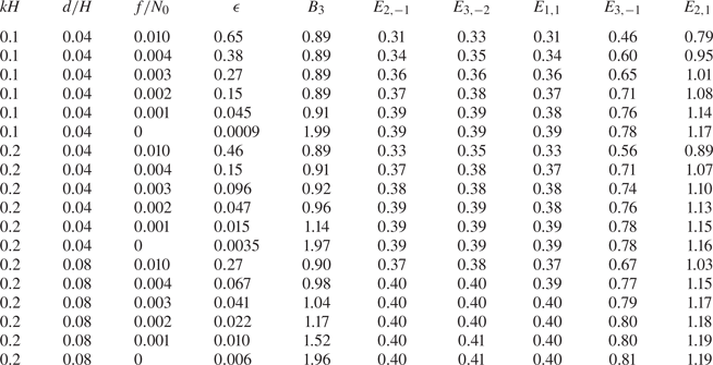
Table 2 lists values of these coefficients as they depend upon the characteristic wavenumber of the internal tide, the e-folding depth of the stratification and the relative Coriolis parameter. The coefficients $E_{ml}$ change little with the variations in $kH$, $d/H$ and $f/N_0$, which is consistent with the long-wave approximations (A2) and (A3). The most significant changes occur for $\epsilon$, which decreases rapidly as $f/N_0$ goes to zero. Consistent with (A7), the coefficient $B_3$ is close to $8/9$ for sufficiently large $f$, but $B_3\simeq 2$ if ${f=0}$.

Table 2.

Non-dimensional coefficients used to compute the evolution of the parent wave with horizontal wavenumber $k$ and its first two superharmonics, $2k$ and $3k$ ($n_\star =3$). The background $N^2$ profile is exponential, given by (3.10). In all cases, $z_0=-0.019H$ and the e-folding depth of the stratification is $d=0.04H$ or $0.08H$, as indicated. The Coriolis parameter, given relative to $N_0\simeq 0.017\ \mbox {s}^{-1}$, ranges from values near Hawaii to ${f=0}$ at the equator as well as the case $f/N_0=0.01$.

The coefficients $\epsilon$, $B_n$ and $E_{ml}$ were also computed for stratification having a surface mixed layer given approximately by (3.11), though to avoid the singularity in ${\rm d}N^2/{\rm d} z$, a hyperbolic tangent function was used to connect the uniform-density layer to the exponential stratification over a distance $0.1 z_0$. The values were found to differ by less than 3 % of the values in the table, consistent with a surface mixed layer having little effect upon the vertical structure function, as shown in figure 1. The coefficients were more sensitive to changing the stratification at depth by weakening the exponential decay at depth of the buoyancy frequency to be more representative of that in the abyss. A detailed exploration of the influence of the structure of the stratification upon the interaction coefficients goes beyond the scope of our present study.

In the special case of the self-interaction of the parent, as determined by the coupling coefficient $E_{11}$, (3.22) shows that this leads to superharmonics only if the fluid is non-uniformly stratified, as has been noted previously (Wunsch Reference Wunsch2015, Reference Wunsch2017; Sutherland Reference Sutherland2016; Varma & Mathur Reference Varma and Mathur2017; Baker & Sutherland Reference Baker and Sutherland2020).

Baker & Sutherland (Reference Baker and Sutherland2020) examined the truncated system of equations involving only the parent self-interaction creating a $2k$-superharmonic, and the $2k$-superharmonic interacting with the parent so as to modify the parent. Respectively, these are given explicitly by

(3.24a,b)\begin{equation} \frac{{\rm d}a_2}{{\rm d}T} - \mathrm{i} \omega a_2 ={-}\mathrm{i}\alpha\,\frac{\omega}{\epsilon}\,E_{11} a_1^2,\quad \frac{{\rm d}a_1}{{\rm d}T} ={-}\mathrm{i}\alpha\, \frac{\omega}{\epsilon}\,E_{2,-1} a_2 a_1^\star.\end{equation}

If the parent wave amplitude is sufficiently small, then the influence of the superharmonic upon the parent can be neglected, in which case $a_1(T)=1$, and the first equation gives $a_2(T)=E_{11}(\alpha /\epsilon ) [1-\exp (\mathrm {i}\omega T)]$. Recalling that $T=\epsilon t$, this shows that the superharmonic grows and decays periodically with frequency $\epsilon \omega$. Also, the $2k$-superharmonic grows to amplitude $\propto \alpha /\epsilon$ with respect to the parent. So the truncation of equations leading to (3.24a,b) is valid provided that $\alpha /\epsilon \ll 1$ (Baker & Sutherland Reference Baker and Sutherland2020).

If $\alpha /\epsilon \gtrsim 1$, then the $2k$-superharmonic can grow to non-negligible amplitude with respect to the parent. If the relative amplitude is fixed, but $\alpha /\epsilon$ is large due to $\epsilon$ being small, then the $2k$-superharmonic would remain large for longer times owing to the smaller beat frequency $\epsilon \omega$. Thus, in this circumstance, it is anticipated that the parent and $2k$-superharmonic should excite higher superharmonics.

Such considerations are not just a theoretical exercise. Although realistic internal tides have small amplitude, circumstances can exist where $\alpha /\epsilon \gg 1$ as a consequence of $\epsilon$ being smaller than $\alpha$. This is particularly likely near the equator where the cut-off frequency $f$ in the dispersion relation goes to zero so that, approaching the limit of very long waves ($kH\rightarrow 0$), $\omega \propto k$. Hence $2\omega (k)=\omega _2\equiv \omega (2k)$, in which case $\epsilon =0$. This is illustrated in figure 2, for which the dispersion relation is computed for mode-1 waves in exponential stratification with e-folding depth $d=0.04H$. At latitudes where $f/N_0=0.008$, $\omega _2$ is moderately offset from $2\omega$ so that $\epsilon \simeq 0.18$ for $kH=0.2$. However, at the equator there is near perfect resonance between the parent mode forcing frequency at $2\omega$ and the natural frequency of the $2k$-superharmonic, as indicated by the low value of $\epsilon \simeq 0.007$. Even for a parent tide with a relatively small vertical displacement amplitude $A_0=5$ m in an ocean of depth $H\simeq 5$ km and stratification with e-folding depth $d\simeq 200$ m, the non-dimensional amplitude $\alpha \simeq A_0/d=0.025$ is larger than $\epsilon$. This implies that progressively higher superharmonics may be excited as internal tides approach the equator.

Figure 2.

For mode-1 waves in stratification given by (3.10) with $d=0.04H$ and $z_0=-0.019H$, plots of the dispersion relation and comparison of $2\omega$ with $\omega _2$, with (a) $f=0.003N_0$, and (b) ${f=0}$. Plots of the corresponding values of $\epsilon$ are shown in (c) for $f=0.003N_0$ and ${f=0}$.

For given stratification, Coriolis parameter and parent wave horizontal wavenumber, the coefficients in (3.21) can be evaluated up to some truncation level $n\leq n_\star$. There are then $n_\star$ coupled equations involving terms with both $m\leq n_\star$ and $|l|< n_\star$. For $\alpha /\epsilon \ll 1$, it is sufficient to choose $n_\star =2$, leading to the pair of equations given by (3.24a,b). For the studies below of the internal tide approaching the equator, $\alpha /\epsilon$ can be much larger than $1$. In these cases, convergence of solutions is found by including superharmonics up to $n_\star =20$.

The system of ordinary differential equations was solved by straightforward time integration with equally spaced time steps ${\rm \Delta} T$. With ${\rm \Delta} T=0.001$ and $n_\star =20$, Matlab integrated the equations over the time of one beat period $2{\rm \pi} /(\epsilon \omega )$ in $\simeq 10$ s of real time on a single 2.7 GHz core. After the solutions were found, the results were rescaled to time $t=T/\epsilon$. The results are shown in figure 3 for cases in which the Coriolis parameter is representative of that near Hawaii and at the equator. Amplitudes are based upon observations of the tide between the neap and spring cycles.

Figure 3.

Time evolution of the amplitudes $a_n$, shown for the parent ($n=1$, solid black lines) and the first five superharmonics ($n=2$, dark blue; $n=3$, medium blue; $n=4$, light blue; $n=5$, dashed green; $n=6$, dashed pale green), computed for (a–c) $f=0.003N_0$ ($\epsilon \simeq 0.096$), and (d–f) ${f=0}$, ($\epsilon \simeq 0.0035$), and for amplitudes (a,d) $\alpha =0.025$, (b,e) $\alpha =0.075$, and (c, f) $\alpha =0.125$. In all cases, $k=0.2H$ and the background stratification is exponential with $N=N_0$ at $z_0=-0.019H$ and $d=0.04H$, and the solutions of (3.21) were found by setting a truncation level of $n_\star =20$.

For the smallest amplitude case with $f=0.003N_0$, only superharmonics with $n\lesssim 3$ grow to significant amplitude, as expected from the small value of $\alpha /\epsilon \simeq 0.26$. These grow and decay in amplitude with the predicted beat period $2{\rm \pi} /(\epsilon \omega ) \simeq 7700/N_0$. The parent wave amplitude barely deviates from its initial value in this case. In all the other cases considered, successive superharmonics are excited, with these growing to significant amplitude while the parent wave amplitude decreases substantially. Notably, the cascade is not monotonic with energy progressively passing to higher superharmonics. Particularly in cases with ${f=0}$, high-order superharmonics rapidly grow to amplitudes larger than $a_2$, but the $2k$-superharmonic can then dominate once more (for example, at time $N_0t\simeq 40\ 000$ if $\alpha =0.025$, as shown in figure 3(d), and at time $N_0t\simeq 23\ 000$ if $\alpha =0.075$, as shown in figure 3e).

It may seem that the competing superharmonics would manifest as a form of wave turbulence. However, as shown below, the superposition of superharmonics in cases with $\alpha /\epsilon \gtrsim 1$ results in the manifestation of a coherent, though not steady, solitary wave train. Finally, we note that the truncated system of equations leads to an energy conservation relation, at least for $n_\star \leq 3$. As shown in Appendix B, even as superharmonics grow at the expense of the parent wave, the sum of the squared amplitudes of all the waves remains close to $|a_1(T=0)|^2=1$.

4. Fully nonlinear solutions

For the purposes of testing the above prediction for the evolution of the internal tide, we performed fully nonlinear numerical simulations and ran diagnostics to compare the evolution of the primary wave amplitude and the amplitudes of each superharmonic.

The fully nonlinear equations were solved using the code described in detail in Sutherland (Reference Sutherland2016). The two-dimensional rotating Boussinesq equations were solved in a rectangular domain with horizontally periodic boundary conditions, and free-slip conditions at the top and bottom of the domain. Explicitly, the code solved the time evolution equations for spanwise vorticity ($\zeta$), spanwise velocity ($v$), and the buoyancy $b$:

(4.1)$$\begin{gather} \zeta_t ={-} u\zeta_x - w\zeta_z - b_x + f v_z + {{Re}}^{{-}1}\,{\mathcal{D}} \zeta, \end{gather}$$

(4.2)$$\begin{gather}v_t ={-} u v_x - w v_z - fu + {{Re}}^{{-}1}\,{\mathcal{D}} v, \end{gather}$$

(4.3)$$\begin{gather}b_t ={-} u b_x - w b_z - N^2 b + {{Re\,Pr}}^{{-}1}\,{\mathcal{D}} b, \end{gather}$$

which are extensions, respectively, of (3.4), (3.1b) and (3.2) to include viscous and diffusive terms. The fields were discretized vertically on an evenly spaced grid, and horizontally in terms of their horizontal Fourier components. The diffusion operator ${\mathcal {D}}$ is a Laplacian operator acting only upon horizontal Fourier components with horizontal wavenumbers greater than $32 k$, in which $k$ is the prescribed horizontal wavenumber of the parent wave. The Reynolds number ${Re}=H^2 N_0/\nu$ was set to $10^5$, and the Prandtl number ${Pr}$ was set to $1$. Although these values are smaller than realistic oceanographic values, they serve to damp numerical noise. Because no diffusivity was applied to disturbances with wavenumbers smaller than $32k$, the parent wave and superharmonics that grow to significant amplitude were not attenuated. At any time, the streamfunction was found by solving $\zeta =-\nabla ^2\psi$ and, from this, $u$ and $w$ were found using (3.3a,b).

The background squared buoyancy frequency in all simulations presented here was exponential, given by (3.10) with $d/H=0.04$ and $z_0=-0.019H$. The code worked in non-dimensional variables, with length and time scales set effectively by prescribing $H=1$ and $N_0=1$. However, for clarity, all variables below are given in units of $H$ and $N_0$.

In the simulations presented here, the horizontal wavenumber was prescribed by ${kH=0.2}$, and the Coriolis parameter was given by either $f=0.003N_0$ or ${f=0}$. For given $k$ and $f$, the vertical structure of the primary wave and its frequency was found by using a Galerkin method to solve (3.9), extracting the lowest frequency solution that corresponds to a mode-1 wave. The polarization relations were then used to initialize the code with the corresponding spanwise vorticity, spanwise velocity and buoyancy fields for one wavelength of the parent wave. In the simulations presented here the maximum vertical displacement amplitude, $A_0$, was set to be $A_0=0.001H$, $0.003H$ and $0.005H$, corresponding to $\alpha =0.025$, $0.075$ and $0.125$, respectively.

We begin by examining the evolution of a relatively small amplitude internal tide with $A_0=0.001H$ in background rotation representative of that near Hawaii, for which $f=0.003N_0$ (for dimensional units, see § 2). For the primary wave with $kH=0.2$, its frequency is $\omega \simeq 0.0085N_0$, and from the frequency of the $2k$-superharmonic, we have ${\epsilon =0.096}$. Because $\alpha /\epsilon \sim 0.26$ is somewhat smaller than $1$, only the lowest superharmonics are expected to grow to significant amplitude, and they are anticipated to beat with a period $2{\rm \pi} /(\epsilon \omega ) \simeq 7.7\times 10^3/N_0$. With $N_0=0.017\ \mbox {s}^{-1}$, this corresponds to a time of $5.2$ days.

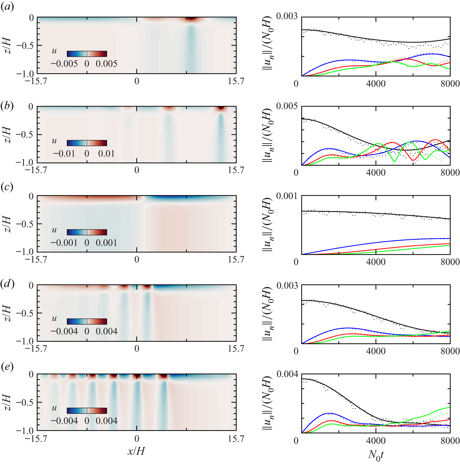
The results of the simulation and comparisons with theory are shown in figure 4. Here we choose to represent the results in terms of the horizontal velocity. A snapshot of the total horizontal velocity is shown at time $N_0t=4000$, corresponding to $2.7$ days (figure 4a). This time is approximately half the predicted beat period of the superharmonics. To reveal more clearly the superharmonics, figure 4(b) plots the horizontal velocity field after subtracting the signal from the primary wave. The snapshots show that the horizontally periodic structure of the parent wave is slightly modulated by the growth of superharmonics. At the surface, the positive (waveward) flow of the total horizontal velocity (figure 4a) extends over a shorter horizontal extent than the negative flow, and it is larger in magnitude than the negative flow. Primarily, this is a consequence of the positive flow of the $2k$-superharmonic interfering constructively with the positive flow of the parent wave, and interfering destructively with its negative flow.

Figure 4.

Supplementary movies are available at https://doi.org/10.1017/jfm.2022.689. From a simulation with $f=0.003N_0$ and $A_0 = 0.001 H$ ($\alpha =0.025$), snapshots at $N_0t=4000$ of (a) the total horizontal velocity field and (b) the horizontal velocity field with the parent wave removed. (c) The simulated (dotted lines) and predicted (solid lines) peak horizontal velocity at $z=0$ associated with the parent wave (black) and superharmonics with $n=2$ (blue), $n=3$ (red) and $n=4$ (green). In all cases, $kH=0.2$ and the background stratification is exponential with $N=N_0$ at $z_0=-0.019H$ and $d=0.04H$.

By Fourier decomposing the horizontal flow at the surface at each time, we compare the time evolutions of the simulated amplitude of the primary wave and its superharmonics with those predicted by theory. Explicitly, from the predicted amplitudes, $a_n(T) =a_n(\epsilon t)$, the magnitude of the surface flow associated with disturbances of horizontal wavenumber $nk$ is $\Vert u_n\Vert = \alpha (\omega d/k)\,|\hat {\psi }^\prime (0)|\,a_n$. Figure 4(c) shows excellent agreement between the simulated and predicted amplitudes of the primary wave and its first two superharmonics. Unlike the theory, the simulations exhibited small-scale oscillations about the predicted parent wave amplitude. These were due predominantly to weak interactions between the parent wave and the induced Eulerian flow, which has a mixed mode-1/mode-2 structure (Sutherland & Yassin Reference Sutherland and Yassin2022). The results show that for the moderately small value of $\alpha /\epsilon$ in this simulation, only the $2k$- and $3k$-superharmonics grow to significant amplitude, and the amplitude of the parent wave decreases only slightly by the time the superharmonics have grown to their largest amplitude at $N_0t\simeq 4000$.

By increasing the parent wave amplitude or by considering the wave evolution at lower latitudes, hence smaller $f$ and larger $\epsilon$, higher superharmonics grow to significant amplitude and the parent wave amplitude decreases non-negligibly. This is shown in the results of five simulations plotted in figure 5. Here, only the total horizontal velocity field is shown in the left-hand snapshots. The right-hand plots show the time evolution of the peak horizontal velocity at $z=0$ for the parent wave and for the $2k$-, $3k$- and $4k$-superharmonics. Higher superharmonics also grow to significant amplitude, but these are not plotted. Focusing on the right-hand plots, we see that the prediction of theory agrees well with the results of numerical simulations. For $\alpha /\epsilon \gtrsim 1$, a superharmonic cascade becomes more evident with higher superharmonics being excited and the parent wave amplitude decreasing significantly. In the cases with ${f=0}$, $\omega \simeq 0.0080$ and $\epsilon \simeq 0.0035$, the predicted beat period resulting from interactions between the parent wave and the $2k$-superharmonic alone is $2{\rm \pi} /(\epsilon \omega )\simeq 2\times 10^5/N_0$ (equivalent to $\simeq 136$ days). Although the range of times examined in figures 5(c–e) is much smaller than the beat period, the superharmonics are observed to grow to substantial amplitude owing to the large values of $\alpha /\epsilon$.

Figure 5.

(There are supplementary movies for (b,e).) As in figures 4(a,b), showing (left) snapshots of the total horizontal velocity field at $N_0t=4000$ and (right) the simulated (dotted) and predicted (solid) time evolutions of the peak surface horizontal velocity for the parent and first three superharmonics for five different cases, with: (a) $f=0.003N_0$, $A_0 = 0.003 H$, $\alpha / \epsilon \simeq 0.78$; (b) $f=0.003N_0$, $A_0 = 0.005 H$, $\alpha / \epsilon \simeq 1.30$; (c) ${f=0}$, $A_0 = 0.001 H$, $\alpha / \epsilon \simeq 7.1$; (d) ${f=0}$, $A_0 = 0.003 H$, $\alpha / \epsilon \simeq 21$; and (e) ${f=0}$, $A_0 = 0.005 H$, $\alpha / \epsilon \simeq 36$.

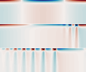
In all cases with $\alpha /\epsilon \gtrsim 1$, the superposition of superharmonics upon the parent wave eventually results in the formation of a solitary wave train. This is characterized by a sequence of localized disturbances with enhanced positive flow near the surface. As shown in the next section, each localized disturbance is associated with a wave of depression, where the isopycnal displacement has maximum downward extent. More waves in the wave train occur and develop more rapidly if $\alpha /\epsilon$ is larger. Thus although multiple superharmonics are excited, their phase relationship results in a coherent wave pattern rather than devolving into a random wave field. Such patterns have also been produced through separate models based upon extensions of shallow-water theory. The comparison between our theory and the shallow-water models is presented next.

5. Comparison with shallow-water theory

Several studies have examined the nonlinear evolution of the internal tide through extensions of shallow-water theory. Here, we compare the predictions of our model with two models, namely the Ostrovsky (hereafter KdV-f) equation (Ostrovsky & Stepanyants Reference Ostrovsky and Stepanyants1989) and the Miyata–Choi–Camassa equations (Miyata Reference Miyata1988; Choi & Camassa Reference Choi and Camassa1999), adapted to include the influence of rotation (Helfrich & Grimshaw Reference Helfrich and Grimshaw2008). The latter model we refer to hereafter as the MCC-f equations.

The KdV-f equation is an extension of the Korteweg–de Vries (KdV) equation that includes the influence of background rotation. Following the notation used above, it is assumed that the vertical displacement field associated with the waves is separable, so $\xi (x,z,t) = \eta (x,t)\,\hat {\psi }(z)$, in which $\eta$ satisfies (Ostrovsky & Stepanyants Reference Ostrovsky and Stepanyants1989)

(5.1)\begin{equation} \frac{\partial}{\partial x} \left[\frac{\partial\eta}{\partial t} + c_0\, \frac{\partial\eta}{\partial x} + \alpha_k \eta\,\frac{\partial\eta}{\partial x} + \beta_k\,\frac{\partial^3\eta}{\partial x^3} \right]=\frac{f^2}{2c_0}\,\eta.\end{equation}

Here, $c_0$ is the long-wave speed found in a system with zero background rotation, and $\alpha _k$ and $\beta _k$ are parameters respectively representing the importance of nonlinearity and non-hydrostatic effects. These are determined explicitly in terms of the vertical structure function $\hat {\psi }$ (Benney Reference Benney1966; Grimshaw & Helfrich Reference Grimshaw and Helfrich2012). Explicitly, in the Boussinesq approximation, we have

(5.2a,b)\begin{equation} \alpha_k =\frac{3}{2}\,c_0\,\frac{\displaystyle \int {(\hat{\psi}^\prime)}^3 \,{\rm d} z}{\displaystyle \int {(\hat{\psi}^\prime)}^2\,{\rm d} z},\quad \beta_k = \frac{1}{2}\,c_0\,\frac{\displaystyle \int \hat{\psi}^2\,{\rm d} z}{\displaystyle \int {(\hat{\psi}^\prime)}^2\,{\rm d} z}.\end{equation}

Given that the scale of $\eta$ is $A_0=\alpha d$, the scale of the nonlinear term relative to the advection term is $d \alpha \alpha _k/c_0 \sim \alpha$, and the scale of the non-hydrostatic term relative to the advection term is $\beta _k k^2/c_0 \sim d^2 k^2$. In these approximations, it is assumed that $\hat {\psi }^\prime$ scales as $1/d$, the inverse characteristic depth of the stratification. The scale of the term representing the influence of rotation relative to advection is $f^2/(c_0 k)^2 \sim (f/\omega )^2$. The approximations leading to (5.1) assume that these three scales are in balance and small: $\alpha \sim (dk)^2 \sim (f/\omega )^2\ll 1$.

The MCC-f equations have been formulated for a two-layer system, in which the upper layer has depth $h_1$, and the density jump between the lower and upper layer is represented by the reduced gravity $g^\prime$. The coupled equations are cast in terms of the upper-layer depth in the presence of an interfacial wave, $h=h_1-\eta$, the horizontal velocity differences between the lower and upper layers in the along-wave direction, $U=u_2-u_1$, and across-wave direction, $V=v_2-v_1$, and in terms of the barotropic transport in the across-wave direction, $Q = v_1 h + v_2 (H-h)$. The barotropic transport in the along-wave direction is assumed to be zero: $u_1 h + u_2 (H-h)=0$. Explicitly, the MCC-f equations are (Helfrich & Grimshaw Reference Helfrich and Grimshaw2008)

(5.3)$$\begin{gather} \frac{\partial h}{\partial t} =\frac{\partial}{\partial x} \left[ Uh\left(1-\frac{h}{H}\right)\right], \end{gather}$$

(5.4)$$\begin{gather}\frac{\partial U}{\partial t} =\frac{\partial}{\partial x} \left[ \frac{1}{2}\,U^2 \left(1-2\,\frac{h}{H}\right) + g'h\right] + f V + (D_2-D_1), \end{gather}$$

(5.5)$$\begin{gather}\frac{\partial V}{\partial t} ={-} U \left[ V\,\frac{1}{H}\,\frac{\partial h}{\partial x} - \frac{\partial V}{\partial x} \left(1-2\,\frac{h}{H}\right) + \frac{\partial Q}{\partial x} + f \right], \end{gather}$$

(5.6)$$\begin{gather}\frac{\partial Q}{\partial t} ={-}\frac{\partial}{\partial x} \left[ U Vh \left(1-\frac{h}{H}\right)\right]. \end{gather}$$

Here, the non-hydrostatic terms are represented by $D_1$ and $D_2$:

(5.7)\begin{equation} D_i = \frac{1}{h_i}\,\frac{\partial}{\partial x} \left[ \frac{1}{3}\,h_i^3 \left( \frac{\partial^2 u_i}{\partial x\,\partial t} + u_i\,\frac{\partial^2 u_i}{\partial x^2} - \left(\frac{\partial u_i}{\partial x}\right)^2 \right) \right],\quad i=1,2, \end{equation}

in which $h_2 = H-h_1$.

In order to compare our model results, for which the background stratification is continuous, to this two-layer model, we use (5.2a,b), in which the vertical structure function is that for a two-layer stratification. Thus we find

(5.8a–c)\begin{equation} c_0 = \sqrt{g^\prime \bar{H}},\quad \alpha_k ={-}\frac{3}{2}\,c_0\,\frac{1}{\bar{H}} \left(1-2\,\frac{h_1}{H_{2L}}\right),\quad \beta_k = \frac{1}{6}\,c_0 H_{2L} \bar{H}, \end{equation}

in which $\bar {H} = h_1 (H_{2L}-h_1)/H_{2L}$, and $H_{2L}$ is the total equivalent depth. These equations can be inverted so that, for given $c_0$, $\alpha _k$ and $\beta _k$ (determined from a system with continuous stratification), we determine the equivalent total depth and upper-layer depth, given respectively by

(5.9)$$\begin{gather} H_{2L} = 4\,\frac{\alpha_k\beta_k}{c_0^2} \left[1 +\sqrt{1+\frac{3c_0^3}{2\alpha_k^2\beta_k}}\right], \end{gather}$$

(5.10)$$\begin{gather}h_1 = 2\,\frac{\alpha_k\beta_k}{c_0^2} + H_{2L}/2. \end{gather}$$

For proper comparison with our theory and the KdV-f equation, the equivalent reduced gravity should be defined based upon the shallow-water speed $c_f$, determined from the dispersion relation that includes the influence of background rotation. Explicitly, $c_f = (\omega ^2-f^2)^{1/2}/k$ and $g' = c_f^2/\bar {H}$.

We solved the KdV-f equation by Fourier transforming $\eta$ in $x$, and then time-evolving the Fourier amplitudes. The MCC-f model was discretized in space with $x$-derivatives approximated by centred second-order finite differences. Both models were advanced in time using a fourth-order Adams–Bashforth–Moulton predictor–corrector scheme. The corrector step was iterated until the magnitude of the relative difference between successive fields was less than a tolerance of $10^{-6}$. These equations were solved in Matlab. Integrating in time up to $N_0t=5000$ was accomplished in seconds using our equations, in minutes for the KdV-f equation, and in about an hour for the MCC-f equations.

We compare the predictions of our theory with the KdV-f and MCC-f predictions for the two cases considered in figures 5(a,d), for which $A_0=0.003H$, and $f=0.003N_0$ and ${f=0}$. For the exponential stratification prescribed for those cases, the corresponding vertical structure functions give the coefficients of the KdV-f equation to be $c_0\simeq 0.040 N_0H$, $\alpha _k\simeq -0.80 N_0$, $\beta _k\simeq 0.00060 N_0H^3$ and $f^2/(2c_0)\simeq 0.00011 N_0$ in the case $f=0.003N_0$. The equivalent parameters for the two-layer system of the MCC-f equations are $H_{2L}\simeq 1.31H$, $h_1\simeq 0.073H$ and $g^\prime \simeq 0.023 N_0^2H$.

The predictions of the three models are shown in figure 6. For both cases with $f=0.003N_0$ and ${f=0}$, there is good qualitative agreement between the three models. All show the emergence of a single localized wave of depression in the case with $f=0.003N_0$, and a solitary wave train in the case with ${f=0}$. Quantitatively, the MCC-f model gives the poorest agreement, predicting that the waves are narrower with more waves in the wave train.

Figure 6.

Comparison of vertical displacement predicted by (a,d) the superharmonic cascade (SHC) model, (b,e) the KdV-f equation, and (c, f) the MCC-f model, in cases with $kH=0.2$, $A_0=0.003$ and (a–c) $f=0.003N_0$, and (d–f) ${f=0}$. For SHC and KdV-f, the background stratification is exponential with $N=N_0$ at $z_0=-0.019H$ and $d=0.04H$. For MCC-f, the equivalent parameters of the two-layer system are computed from the corresponding coefficients computed for the KdV-f equation. In all cases, the displacement is plotted at evenly spaced times, as indicated in (d), with successive times being vertically offset. The plots are given in a frame of reference moving with the phase speed $c_p$ of the parent wave.

Despite these minor discrepancies, it is reassuring that our superharmonic cascade model reproduces the results of the well-established shallow-water models when the parameters governing the amplitude and the importance of non-hydrostatic effects are in the appropriate regime.