1 Introduction
As mobile GPS is becoming widely available in the market, coupled with publicly accessible online maps (e.g. Google Maps), route planning and direction that show a desirable route from a departure point to the destination has grown to be one of the most popular navigation applications these days (Safar, Reference Safar2005; Xuan et al., Reference Xuan, Zhao, Taniar and Srinivasan2008, Reference Xuan, Zhao, Taniar, Safar and Srinivasan2011). The recommended routes by these systems are normally those with the shortest distance. Using these systems, users could easily adjust the turning points at any intersections, which alter the initial route to become a user-preferred route. More advanced navigation systems can even predict the traveling time of the chosen route. Route planning can be regarded as a successful application of shortest distance algorithms, like Dijkstra algorithm (Dijkstra, Reference Dijkstra1959).
Recently, route search has been extended to include locations to be visited along the planned route (Huang & Jensen, Reference Huang and Jensen2004; Terrovitis et al., Reference Terrovitis, Bakiras, Papadias and Mouratidis2005; Yoo & Shekhar, Reference Yoo and Shekhar2005; Zhang, Reference Zhang2008; Zhao et al., Reference Zhao, Xuan and Taniar2013; Kanza et al., Reference Kanza, Safra, Sagiv and Doytsher2008b; Zhao et al. Reference Zhao, Xuan, Rahayu, Taniar, Safar, Gavrilova and Srinivasan2011; Kanza et al., Reference Ilarri, Mena, Illarramendi, Yus, Laka and Marcos2008a, Reference Kanza, Safra and Sagiv2009). The aim was to find the shortest distance, and sometimes the most reliable route, that covers all user-defined locations or places. Although this is certainly useful, it is often impractical, due to a couple of reasons: (i) each location or place, which are normally a spatial business entity (e.g. bank, dry cleaner, supermarket) has the opening hours—this implies that when this place is visited, it must be during their business hours; and (ii) the traveling time from one location to another needs to be considered, as in many cases, traveling time is more useful than the distance alone. Hence, in order to make route planning over visiting locations, one must take into account these two constraints. In this paper, we refer to these constraints as Time Constraints. Therefore, our paper focuses on route search over multiple locations taking into consideration time constraints.
It is therefore imperative to assume that the route or path that arrives on the location outside the operation hour is considered as an invalid path. This problem exists in daily life, whereby we sometime have to choose a longer path to go back and forth places just to meet the business hours of one location before its closing time. Hence, we need to draw time constraints into our proposed methods.
Route search over multiple locations is often assumed to be the problem of kNN or continuous kNN in spatial and mobile databases (Roussopoulos et al., Reference Roussopoulos, Kelley and Vincent1995; Papadias et al., Reference Papadias, Zhang, Mamoulis and Tao2003; Kolahdouzan & Shahabi, Reference Kolahdouzan and Shahabi2004; Safar, Reference Safar2005). There is a huge distinction between kNN and route search. kNN finds spatial objects that closest located to the query point, without considering the path that needs to be established as the user has to visit each objects in the query result. Because of this, existing work on kNN is inapplicable to solve route search problems. Our previous work on incremental kNN (called ikNN; Zhao et al., Reference Zhao, Xuan and Taniar2013) attempts to solve route search problem whereby it could find the shortest distance to cover k number of homogenous type of locations—however, it does not consider time constraints, nor heterogenous multiple types of locations.
In this paper, we focus on two problems of route search over multiple heterogenous locations: one for fixed locations, and the other for flexible locations. Fixed locations refer to predetermined locations by the user, such as Citibank on a specific location, Pharmore pharmacy on a specific location, etc. In this case, not only specific business entity is specified, such as Citibank and not any bank, or Pharmore pharmacy and not any pharmacy, but also the specific location, such as Citibank on 180 High Street, or Pharmore pharmacy on 25 Cure Road, etc. Hence, a Route Search over Fixed Locations (our proposed algorithm is then called RFix) finds the most efficient route to visit the user-defined fixed locations in a non-predefined order.
Flexible locations, on other hand, refer to predetermined location types, are not the exact location itself. For example, if user wants to visit a pharmacy, which can be the pharmacy anywhere; or to visit Citibank, but can be in any branch. So, a route search over flexible locations, for example, is to find the most efficient route to visit Citibank, a pharmacy, etc. in a non-predefined order. Our proposed algorithm for Route Search over Flexible Locations is abbreviated as RFlex. Both RFix and RFlex use the travel time network to estimate the travel time between any two locations, as well as using the time constraints imposed by not only the operating hours of each location, but also the traveling time itself.
2 Related work
Some variations of route search have been investigated in earlier works (Pearson & Guesgen, Reference Pearson and Guesgen1998; Huang & Jensen, Reference Huang and Jensen2004; Ehliar & Liu, Reference Ehliar and Liu2005; Terrovitis et al., Reference Terrovitis, Bakiras, Papadias and Mouratidis2005; Yoo & Shekhar, Reference Yoo and Shekhar2005; Zhang, Reference Zhang2008; Zhao et al., Reference Zhao, Xuan and Taniar2013; Kanza et al., Reference Ilarri, Mena, Illarramendi, Yus, Laka and Marcos2008a; Kanza et al., Reference Kanza, Safra, Sagiv and Doytsher2008b). In Yoo and Shekhar (Reference Yoo and Shekhar2005) and Huang and Jensen (Reference Huang and Jensen2004), they try to find the route with smallest deviation to visit a new point when user travels a pre-defined route. Zhao et al. (Reference Zhao, Xuan and Taniar2013) and Terrovitis et al. (Reference Terrovitis, Bakiras, Papadias and Mouratidis2005) have single type of interest points and no time constraint involved. Considering the inaccuracy and incomplete issues, some works assigned scores or probabilities to each locations and the result path should pass the locations with high probabilities (Kanza et al., Reference Kanza, Safra, Sagiv and Doytsher2008b, Reference Kanza, Safra and Sagiv2009). In our query, the criteria is the path with shortest travel time which is different from shortest path (Xuan et al., Reference Taniar and Rahayu2011). In addition, in some route search, the path can go through multiple locations of the same type (Kanza et al., Reference Kanza, Safra, Sagiv and Doytsher2008b, Reference Kanza, Safra and Sagiv2009) while our path only visit one location for each type. Moreover, even if a lot of different constraints have been studied, there is no paper that draws time constraint into Route Search query. Although our proposed methods are significantly different from existing works (Ehliar & Liu, Reference Ehliar and Liu2005), they are still worth to be reviewed as they become our motivation.
2.1 Route search query
Route search query was proposed by Yaron Kanza et al. in 2008 (Kanza et al., Reference Kanza, Safra, Sagiv and Doytsher2008b). There are three semantics covered in this paper, such as given start point, end point and all types of user interests, the first semantics is to return the shortest route that goes via all relevant entities. A second semantics is to find the most-profitable route, which is the route having the highest accumulative relevance and the length of the route is within the given limit. A third semantics is to compute the most-reliable route, which goes through as much higher relevant entities as possible and the length of the route is within the given limit.
Route search query uses greedy insertion from both start point and end point to find the final path. In route search, similar as our methods, multiple location types are concerned and the final path must pass one location of each type in any order.
Outstanding Problems:
• Route search query chooses multiple criteria such as shortest distance, highest relevance or more relevant entities with higher relevance. While we choose the shortest travel time because we draw time constraint into the query and shortest distance cannot guarantee the shortest travel time.
• Route search query has a pre-defined path length limit while our methods are indifferent to travel distance.
• Route search query pre-defined the start and end point while our methods only give the start point.
• Route search query does not concern arriving time for any interest point while the optimum path of our methods should meet the time constraint of each type.
2.2 Incremental kNN
Incremental k nearest neighbor (iKNN; Zhao et al., Reference Zhao, Xuan and Taniar2013) is given a set of candidate interest points to find the shortest path, which starts at query point and goes through k interest points. For example, find the shortest path, which goes through three restaurants from q. It is a novel kNN because the result is the shortest path and the interest points are visited one by one. While it is not a Route Search query neither because all candidate interest points are single type, while our Route Search query involves multiple types, which needs access to different data structures such as multiple Network Voronoi Diagram (Okabe et al., Reference Okabe, Boots, Sugihara and Chiu2000; Kolahdouzan & Shahabi, Reference Kolahdouzan and Shahabi2004; Zhao et al., Reference Taniar and Rahayu2009) and the result path must cover every type.
iKNN uses network expansion as Incremental Network expansion (INE). In the process of network expansion, iKNN records all expansion branches until one path is full of k interest points. The path is set as the boundary. Continue to do the expansion, once there is a path shorter than the boundary; shrink it until all possible branches are expanded out of boundary. iKNN is similar with our proposed methods, such as both methods have a boundary identifier ( $$\[--><$> D/{{T}_{max}} <$><!--$$
) to shrink the expansion scope and numbers of points to be visited are given.
Outstanding Problems:
• iKNN considers all interest points as single type while our methods consider multiple location types.
• iKNN does not concern arriving time constraint for any interest point while the optimum path of our methods should meet the time constraint.
2.3 Additional specifications
Before we move on to the proposed methods, more specifications are described and compared with other existing works:
• Why cannot kNN solve Route Search query?
kNN cannot guarantee all locations to be fully covered, since the distance from query point to all interest points is the only criteria, and not the complete path.
• What are the differences between incremental kNN and Route Search query?
In incremental kNN, all interest points are considered as single type while in route search query, there are multiple types of interest points and the optimal path should go through all types of interest points.
• Can multiple 1_NN find all interest points?
If we use 1_NN to find the nearest neighbor until all types have been found, there is high possibility that the final path is not the most optimum one. The first nearest interest point may lead to a further distance to other interest points, as a result, it does not yield an optimum path. This is a common local minimal problem in scheduling.
• Why does the shortest time need to be used instead of the shortest distance?
Since the problem of answering Route Search queries is a generalization of the traveling salesman problem, it is unlikely to have an efficient solution, that is, there is no polynomial-time algorithm that solves the problem (unless P = NP; Kanza et al., Reference Ilarri, Mena, Illarramendi, Yus, Laka and Marcos2008a). Hence, as a solution, this paper incorporates time constraint in order to prune as many expansion branches as possible and makes the query more realistic. If we use time constraint to prune the expansion branch, choosing traveling time as criteria is straightforward and can be adjusted to different travel time period.
3 Proposed methods
In this section, our proposed Route Search for fixed locations (RFix) and flexible locations (RFlex) are described. In each method, the query is given first followed by detailed explanations of the key issues, then after listing the algorithm, an example will illustrate the processing steps. As travel time is chosen as criteria, travel time network needs to be introduced first.
In Travel time network (Ku et al., Reference Ku, Zimmermann, Wang and Wan2005), the measurement between nodes is the travel time instead of network distance. This is often more desirable because under certain conditions travel time is more meaningful than network distance, such as whether the path arriving at locations within their operating hours depends on the travel time, not travel distance. In this paper, we use the average travel speed in routine profile to estimate the approximate travel time. Figure 1 gives an example of a travel time network. We assume that the average travel time for each road segment is read from the traffic profile.
Road network vs. travel time network

3.1 Route search for fixed locations (RFix)
When the query is a RFix, this query can be categorized as RFix. Example 1 illustrates a RFix query. It can be expressed as follows: Start at q at 4:30pm, find the optimum path whose travel time is shortest and this path should visit A, B, C and D between 9:00am–5:00pm, 9:00am–5:30pm, 4:30pm–5:40pm and 6:00pm–6:30pm, respectively. Now we can treat q, A, B, C and D as locations and invoke our proposed method RFix to find an optimum path. The pruning conditions are explained as follows:
Example 1:Secretary will leave her office at 4:30pm. She has a plan to do:
• Fetch a suit from dry cleaner A and A's trading time is 9:00am–5:00pm.
• Fetch a contract from Company B and B's open hours are 9:00am–5:30pm.
• Send a report to manager's apartment C and he is at home 4:30pm–5:40pm.
• Pick up her son from kindergarten D and D's pick up period is 6:00pm–6:30pm.
3.1.1. RFix definition
The RFix query can be formally defined like this:
Definition 1 RFix is a route search query consisting of: Input: Type Set T = {t 1, t 2, …, tn}, Locations set P = {p 1, p 2, …, pn}, ∀ pi ∈ ti. Output: A Path l which goes through all ps in P and distancel is the shortest.
3.1.2 Pruning conditions
Since the problem of answering Route Search queries is a generalization of the traveling salesman problem, it is unlikely to have an efficient solution, hence an efficient pruning method is crucial. With the prune conditions, the candidate permutation is greatly reduced and that is the basis of our solutions. Two pruning conditions are discussed in this section. First, definition for Invalid Path and Valid Path are introduced here.
Definition 2 A path is invalid when at least one location's arriving time followed by this path is out of its operating hours; otherwise if it visits all user defined location types, it is a valid path.
 $$\left \matrix {{\exists {{P}_i}} \hfill \cr{Path(q\, \rightarrow \,{{P}_1}\, \rightarrow \, \ldots \, \rightarrow \,{{P}_i}\, \rightarrow \, \ldots \, \rightarrow \,{{P}_j})} \hfill \cr{T(q\, \rightarrow \,{{P}_1}\, \rightarrow \, \ldots \, \rightarrow \,{{P}_i})\, \notin \,OperatingHour({{P}_i})} \hfill \\\end{}} \right\}\, \Rightarrow \,Invalid(q\, \rightarrow \,{{P}_1}\, \rightarrow \, \ldots \, \rightarrow \,{{P}_i}\, \rightarrow \, \ldots \, \rightarrow \,{{P}_j})$$
Pruning condition 1: non-reversible visiting sequence. If q → Pi → Pj is a valid path while q → Pj → Pi is an invalid path as in Equation (1), (Pi, Pj) have non-reversible visiting sequence (q → Pi → Pj). Hence, any solution visiting Pj before Pi should be pruned.
 $$\left \matrix{ {valid(q\, \rightarrow \,{{P}_i}\, \rightarrow \,{{P}_j})} \hfill \cr {Invalid(q\, \rightarrow \,{{P}_j}\, \rightarrow \,{{P}_i})} \hfill \cr {Type({{P}_i}),\,Type({{P}_j})\, \subseteq \,LocationTypelist} \hfill \\\end{}} \right\}\, \Leftrightarrow \,P_{{i{\nleftarrow}}}^{\ \,{ \rightarrow }} {{P}_j}$$
Proposition 1 Given a query point q and two locations P 1and P 2
 $$\left \matrix{ {StartTime\, \gt \,OpenTime({{P}_1})} \hfill \cr {StartTime\, \gt \,OpenTime({{P}_2})} \hfill \cr {CloseTime({{P}_1})\, \lt \,CloseTime({{P}_2})} \hfill \cr {Invalid(q\, \rightarrow \,{{P}_1}\, \rightarrow \,{{P}_2})} \hfill \\\end{}} \right\}\,{\nRightarrow}\,Invalid(q\, \rightarrow \,{{P}_2}\, \rightarrow \,{{P}_1})$$
Proof If CloseTime(P 1) < CloseTime(P 2) which means P 1 closes earlier than P 2, it is possible that (P 1, P 2) have a non-reversible visiting sequence q → P 1 → P 2 because if we visit P 2 first, when we arrive P 1, it is already closed. It is self-evidence.
If CloseTime(P 1) < CloseTime(P 2) and q → P 1 → P 2 is invalid, we will prove that we cannot conclude q → P 2 → P 1 is invalid by contrapositive.
 $$\left. \matrix{ {T(q,{{P}_1}) + T({{P}_1},{{P}_2}) \approx 2\,\times\,T(q,{{P}_1})\, \gt \,CloseT({{P}_2}) \Rightarrow Invalid(q\, \rightarrow \,{{P}_1}\, \rightarrow \,{{P}_2})} \hfill \cr {T(q,{{P}_2}) + T({{P}_2},{{P}_1}) \approx T(q,{{P}_1})\, \lt \,CloseT({{P}_1}) \Rightarrow Valid(q\, \rightarrow \,{{P}_2}\, \rightarrow \,{{P}_1})} \hfill \\\end{}} \!\!\right\} \Leftrightarrow \,\exists P_{{2{\nleftarrow}}}^{\ \,\,{ \rightarrow }} {{P}_1}$$
□
Pruning condition 2: Invalid sub-paths make the entire path invalid. Any permutation containing invalid sub-path should be pruned. See Proposition 2.
 $$\left \matrix { {Invalid(q\, \rightarrow \,{{P}_i}\, \rightarrow \,{{P}_j})} \hfill \cr {StartTime\, \gt \,Max(OpenTime({{P}_i}),OpenTime({{P}_j}))} \hfill \\\end{}} \right\}\, \Rightarrow \,Invalid(q\, \rightarrow \, \ldots \, \rightarrow \,{{P}_i}\, \rightarrow \, \ldots \, \rightarrow \,{{P}_j})$$
Proof
$$\left \matrix{ {T(q\, \rightarrow \,{{P}_i}\, \rightarrow \,{{P}_j})\, \gt \,CloseTime({{P}_j})} \hfill &#x0026; {} \hfill \cr {T(q\, \rightarrow \,\ldots\, \rightarrow \,{{P}_i}\, \rightarrow \,{{P}_k}\, \rightarrow \,{{P}_j})\, \gt \,T(q\, \rightarrow \,{{P}_i}\, \rightarrow \,{{P}_j})} \hfill &#x0026; {} \hfill \cr {{{P}_k}\, \ne \,{{P}_i}\, \ne \,{{P}_j}} \hfill &#x0026; {} \hfill \\\end{}} \right\}}\\\end{}$$
□
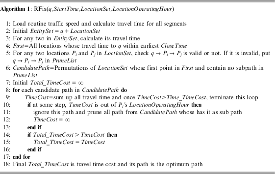
The RFix method is processed in the following steps and the algorithm is shown in Algorithm 1.
RFix(q,StartTime,LocationSet,LocationOperatingHour)
First, depending on current time period, retrieve the traffic speed and calculate the time cost between any two locations in the set, which includes the query point and all fixed locations. The process is similar to Dijkstra algorithm if the weight between entities are travel time cost.
Second, find all locations in First whose travel time to q is within the earliest close time, meaning that if the path goes to the other points first, the path already misses the location with the earliest close time. After checking its arriving time is in the operating hours, put it into First. As a result, First holds all possible locations which can be the first visited.
Third, for any two locations (Pi and Pj), calculate whether q → Pi → Pj match i, j’s operating hours or not. If not, record q → Pi → Pj into PruneList. Then generate all permutations of visiting sequence whose first visiting node is in First and do not include any sub path in PruneList.
Fourth, for each candidate path, sum up its cost time and compare the time with time constraint. Once it exceeds the time constraint, ignore it and filter the other path who has the same sub path. For example if q → P 1 → P 2 → P 3 fails to match time constraint and when query starts, P 1, P 2 and P 3 have opened already, q → P 1 → P 5 → P 2 → P 6 → P 3 should be pruned as well.
Finally, compare the time cost of the path left and choose the optimum one.
3.1.3 A case study
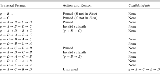
To clarify the algorithm, a case study (see in Figure 2) is presented. This case study is based on Example 1. Table 1 shows the RFix filter process.
RFix example. RFix =Route Search for fixed locations
RFix filter process
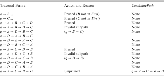
Firstly, q → B → A will make A over its close time, so B is not in the First list. The same goes for C.
Secondly, according to Proposition 2,  $$\[--><$> q\, \rightarrow \,{{C}_{4:55pm}}\, \rightarrow \,{{B}_{5:19pm}} <$><!--$$
is valid and
 $$\[--><$> q\, \rightarrow \,{{B}_{5:18pm}}\, \rightarrow \,{{C}_{5:42pm}} <$><!--$$
cannot meet C close time (5:40pm), so
 $$\[--><$> B_{{\nleftarrow}}^{ \rightarrow } C <$><!--$$
. Add q → B → C into PruneList.
Thirdly, the same as second step, add q → D → B into PruneList.
Finally, generate the permutation whose first node is A or D (in First) and does not contain sub path in PruneList. In this case, only one path lists. After checking this path satisfy all time constraints, it is the result of this query (q → A 4:35pm → C 5:03pm → B 5:27pm → D 6:22pm).
3.2 Route search for flexible locations (RFlex)
When the user has pre-defined the location types whereby any locations of that type can be visited, this query can be categorized as RFlex, see example 2. As there are no fixed locations, we should distill the location types first according to the query specification. Then the query can be summarized as finding an optimum path which goes through these types within the time constraint.
Example 2: Secretary will leave her office at 4:30pm. She has a plan to do:
• Deposit a cheque in any bank and all banks’ trading hour is 10:00am–5:00pm.
• Buy a printer in any shop and all shops’ operating hours is 11:00am–5:30pm.
• Post a letter in any post office and posts’ trading hour is 10:00am–5:40pm.
• Buy some medicine in any pharmacy and all pharmacies’ trading hour is 10:00am–6:30pm.
3.2.1 RFlex definition
The RFlex query can be formally defined like this:
Definition 3 RFlex is a route search query consisting of: Input: Type Set T = {t 1, t 2, …, tn}, Locations set P = {p 1, p 2, …, pm}, m > n. Type(pi, … ,pj) =tk ∈ T Output: A Path l which goes through ps and ps cover all types in T. Also distancel is the shortest.
3.2.2 Pruning conditions
Traditional Route Search query is an NP complete problem and the focus of this section is how to use time constraint to prune most of expansion branches. Basically, our pruning conditions prune the path which leads to unreachable point or which is out of time.
Proposition 3 (Pruning condition 3):If P satisfies Equation 7, P_NN holds Ps’ nearest NN of all types in unvisited_type, P, leads to a unreachable point. P will be pruned out candiate_next set (see Algorithm 3).
 $$\left \matrix { {TimeCost(P,P\_NN(Typ{{e}_i}))\, + \,TimeCost(q,P)\, \gt \,CloseTime(Typ{{e}_i})} \hfill \cr{Typ{{e}_i}\, \in \,unvisited\_type} \hfill \\\end{}} \right\}\, \Rightarrow \,Unreachable(P)$$
Proof
$$ \left \matrix { {CloseTime(Typ{{e}_i})\, \lt \,TimeCost(P,P\_NN({{P}_k})\,\leqslant \,TimeCost(P,\forall {{P}_i})} \hfill \cr{{{P}_i}\,\amp \,{{P}_k}\, \in \,Typ{{e}_m}\, \in \,unvisited\_type} \hfill \\\end{}} \right\}}}$$
□
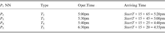
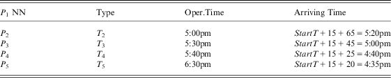
Example of Pruning condition 3: Figure 3 is a case study of Example 2. Suppose P 1 is the candidate_next point, according to Proposition 3, whether it should be pruned or not depends on the data in Table 2. Pi is the nearest neighbor of P 1 in Typei. As P 1's type is T 1, then unvisited_type = T 2, T 3, T 4, T 5. Find P 1's NN for each type in unvisited_type (Column 1 in Table 2). We can easily tell that P 2 is out of OperatingHours of Type 2, in other words, P 1 leads unvisited type T 2 unreachable. Consequently P 1 cannot be the candidate_next point.
Pruning condition 3
Proposition 3 Demo for RFlex
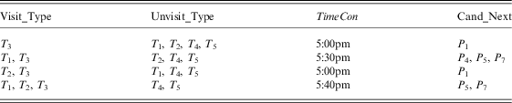
Proposition 4 (Pruning condition 4):Locations whose types are in unvisited_Type within TimeCon (see equation 9) can be in candidate_next. Equation 10which collects the candidate_next set can prune lots of interest points.
 $$StartTime\, \gt \,\mathop {\rm max}\limits_{\forall i\, \in \,n} (OperatingHours({{P}_i}))\, \Rightarrow \,TimeCon\, = \,{\rm max}(CloseTime(unvisited\_Type))$$
 $$candidate\_next(P)\, = \left \{\matrix {{\;\forall {{P}_i}} \hfill \cr {\;TimeCost(P,{{P}_i})\, \lt \,TimeCon} \hfill \cr {\;Type({{P}_i})\, \in \,unvisited\_Type} \hfill \\\end{}} \right.$$
Proof Suppose when we start the query, all locations are open, TimeCon should be set as the earliest close time in unvisited_Type as if the earliest close time type has not been visited, the locations that are going to be visited must be finished ahead of the earliest close time, otherwise when expanding to the earliest close time type, the arriving time is already out of the time constraint.
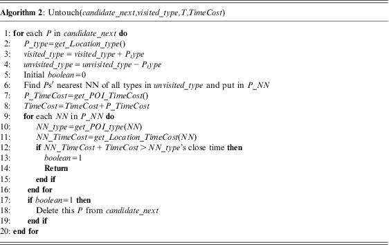
Untouch(candidate_next,visited_type,T,TimeCost)
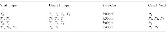
Example of Pruning condition 4: Referring to Figure 4 and Table 3, suppose P 3 of T 3 is the current expansion point. In Table 3, each line represents one scenario as the unvisited_Type is different. Take the first line as an example, if the only visited type is T 3, then the unvisited_Type = {T 1, T 2, T 4, T 5} and TimeCon = T 1's close time = 4:30pm. Only P 1 can be the candidate_next point because all of the other points are out of TimeCon according to Proposition 4. Algorithm 3 shows the process of how to find candidate_next points, which satisfies pruning conditions 4.
Pruning condition 4
Proposition 4 Demo for RFlex
CandidateNext(P,visited_type,T,TimeCost)

With these two pruning conditions, most expansions branches have been pruned. Although the execution time could potentially be exponential in the worst case because the pruning strategy is only heuristic, the pruning conditions do improve the performance significantly.
The detailed steps are shown as follows:
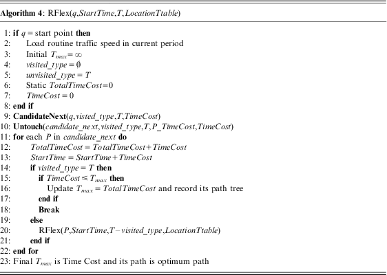
First, initialize Tmax as ∞ and it is the boundary identifier, which will hold the final result. Initialize the visited_type as ∅, which is the collection of the location types that have been visited. Also, initialize T as all location types of user interest.
Second, according to the current time period, load routine traffic speed and get all interest points around q whose travel time to q is within TimeCon. Collect them in a set call candidate_next and prune these points using pruning condition 3.
Third, for any point in candidate_next, do the following. Remove any P in candidate_next, add P's type into visited_type. Then repeat the second step until all types have been visited. Once this path's cost time is shorter than Tmax, replace Tmax with its cost time.
Finally, Tmax is the shortest travel time and its path is the optimum path.
The algorithm of RFlex is shown in Algorithm 4.
4 Performance evaluation
We used network and interest points data in Los Angeles in our experiments. We extracted eight different types of interest points to simulate different location types, including 15 parks, 29 coffee lounges, 31 bank branches, 54 hotels, 78 post offices, 158 pharmacies, 283 shops and 597 restaurants and all interest points are normally distributed.
In our experiments, we varied the following parameters: the number of location types, the congestion level (speed), density of interest points and the average time interval between locations to observe their effects on average processing time, memory as well as their improvement compared with the exhaustive traversal of all permutation approach.
4.1 Experimental results of RFix
Since number of locations highly influences our method's performance, we test the processing time (Figure 5(a)) and memory (Figure 5(b)) for two to eight locations based on three different traffic status (low, medium and high congestion).
Time and memory comparison between different number of locations and traffic status in RFix and time and memory incremental ratio when adding more locations. RFix =Route Search for fixed locations
RFlex(q,StartTime,T,LocationTtable)
From Figure 5(a) and Figure 5(b), we can easily tell that with the increasing number of locations, the processing time and memory are direct proportional to the number of locations. In addition, when the congestion level increases from low to high, the speed decreases at the same time and it causes a slightly increase of the processing time and memory. When it is extremely congested, the processing time and memory will cost ~8–14% more than the lower level. While adding one more location into query list, there will be exponential growth in processing time and logarithmic growth in memory size required, referring to Figure 5(c) and Figure 5(d) when location number is greater than 8, the performance scale increases sharply.
Without using our method, RFix query can be solved by traversing all permutations at the cost of processing time and memory size. To improve its performance, we have proposed two pruning conditions in this paper. Figure 6(a) and Figure 6(b) give the performance comparison in processing time and memory between with and without pruning conditions. Figure 6(c) highlights the advantages of our pruning conditions.
Proc. time and memory comparison between RFix and traversal methods. RFix =Route Search for fixed locations
To sum up, with the increasing number of locations, our methods with pruning conditions outperform the traversal methods in both processing time and memory aspects especially when the location number is greater than 3.
In this paper we include time constraint into Route Search query, normally user will follow rules: earliest close, first visit. In other words, the path is sorted by the close time sequence and this path is abbreviated as PDT. PDT ratio is the possibility that PDT is the optimum path (Equation 11). In this section, we analyze factors that will affect the visiting path, see Figure 7(a) and Figure 7(b).
PDT is optimum (RFix) ratio. RFix = Route Search for fixed locations
 $$PDT\,\,Ratio\, = \,\frac{{number\,\,of\,\,times(PDT\, = \,optimum\,\,path)}}{{n\,\,times\,\,experiments}}$$
Before analyzing our experiment results, first we define a factor called Travel distance span in average Time interval to objects Distribution region (TTD). Object Distribution Region (ODR) is the size of the region that user can arrive within the last location close time. TTD represents the coverage percentage of ODR in average time interval between locations.
 $$ODR\, = \,\pi {{(({\rm max}\,CloseTim{{e}_i}\,{\rm{ - }}\,StartTime)\times\,\overline{t} )}^2} $$
 $$TTD\, = \,\frac{{{\bigg( {\mathop{\sum}\limits_{i\, = \,1}^n (CloseTim{{e}_n}\,{\rm{ - }}\,CloseTim{{e}_{n\,{\rm{ - }}\,1}}} \big)/n} \bigg)\times\,\overline{t} }}{{ODR}}$$
Figure 7(a) shows that low travel speed will lead a high possibility that an optimum path is PDT until the average interval increases to 2 h or more, while high travel speed leads more possibility that optimum path is different from PDT when the average interval is >0.4 h. This result is in conformity with a common sense as if the average time interval between locations is small and speed is relatively slow, visiting locations along the close time sequence has a higher possibility to meet the time constraint because if we visit the later close time location, there will be a high possibility that we cannot catch the earlier location, and vice versa.
Figure 7(b) illustrates that if TTD increases, which means its coverage percentage in average time interval increases, the possibility that PDT is the optimum path drops. The percentage remains stable until TTD increases to around 1.
4.2 Experimental results of RFlex
For RFlex query, the average time interval between locations is a factor that affects the visiting sequence. People generally believe that if the average time interval between locations is large, the performance falls badly. While Figure 8(a) and Figure 8(b) prove that this conjecture is not correct because our RFlex goes down to get the first path and this path is set as boundary. As a result, the processing time is nearly linear and the memory decreases a little with the increasing average time interval between locations. As a result, our approach perform well even there is no time constraint when the number of locations remains constant.
RFlex in different time interval. RFix = Route Search for fixed locations
The processing time and memory will steeply increase with the increasing number of locations and this is already proven in RFix. In this section, we compare the differences between high density distributed objects (e.g. restaurant, density = 0.09375) and low density distributed objects (e.g. parks, density = 0.0024). In our experiments, we test the processing time and memory for locations numbers from 2 to 7 refer to Figure 9(a) and Figure 9(b) for low and high densities of locations.
Processing time and memory comparison for different object densities in RFlex and Processing time and memory incremental ratio when adding more location. RFix =Route Search for fixed locations
Figure 9(c) and Figure 9(d) show that if Route Search query involves more low density objects, with the increasing number of locations, the processing time and memory do increase, but much slower than the high density objects.
5 Conclusion and future work
This paper proposes novel Route Search methods with time constraint involving multiple object types. RFix provides a solution to users if they want to find the shortest travel time path for multiple location types and the locations of these types are fixed. RFlex helps users to find the shortest travel time path if the locations of these types are flexible. Both queries do not concern visiting sequence of objects subject to the final path as long as they arrive at each location within its operating hours. In our method, network Voronoi Diagram is used to find the candidate next visiting point within certain time range and it enriches the content of our mobile navigation system and gives more benefits to mobile users as well.
We performed several experiments to measure the performance of RFix and RFlex in different network conditions and object distributions. In general, our algorithm performs better if the number of locations is small. If the number of locations is <7, the performance is acceptable no matter how complex the road condition is and how objects are distributed. However, as expected, if the number of locations is >7, the processing time and memory increase sharply. In addition, if the average location close time interval is large, our optimum path has a high possibility that it is not PDT, which means discarding PDT and using our methods can give users a better path choice. Lastly when comparing RFix with the traditional traversal permutation method, it performs better and the advantage becomes obvious when number of locations increase up to 4.
In the future, we are going to incorporate intelligence techniques and context-aware in mobile navigation and mobile query processing (Waluyo et al., Reference Waluyo, Srinivasan and Taniar2003, Reference Waluyo, Srinivasan and Taniar2004; Goh & Taniar, Reference Goh and Taniar2004a, Reference Goh and Taniar2004b; Taniar & Rahayu, 2013). In addition, Route Search combined with dynamic query point or locations will also be investigated (Taniar & Rahayu, Reference Taniar and Rahayu2002, Reference Taniar and Rahayu2004; Waluyo et al., Reference Waluyo, Srinivasan and Taniar2005b; Taniar & Goh, Reference Taniar and Goh2007; Mammeri et al., Reference Mammeri, Morvan, Hameurlain and Marsit2009). Performance in mobile query processing is always an issue, we plan to examine more thoroughly the performance issues of mobile query processing including the use of data broadcast techniques (Ilarri et al., Reference Ilarri, Mena, Illarramendi, Yus, Laka and Marcos2012).
Acknowledgments
This research has been partially funded by the Australian Research Council (ARC) Discovery Project (Project No: DP0987687).