Introduction

We have closely examined a potential Mars polar-cap mission called Cryoscout. It relies on a cylindrical, tethered subsurface descent vehicle called the Cryobot (Reference FrenchFrench and others, 2001; Reference Zimmerman, Anderson, Carsey, Conrad, Engelhardt, French and HechtZimmerman and others, 2002), a thermal probe that combines the passive heating of the Philberth Probe (Reference AamotAamot, 1968; Reference Philberth and SplettstoesserPhilberth, 1976) with the forced heat transfer of hot-water drilling (Reference Engelhardt, Kamb and BolseyEngelhardt and others, 2000) through a heated jet in the nose. In the design and development of the Cryobot for this mission, key factors included the low ambient temperature of Mars ice, dust inclusions, overpressure protection, instrument integration, cleanliness and the initial entry into the ice.

The science data of the mission will be acquired at the surface, with an optical fiber in the tether, and on the Cryobot. The surface station will obtain meteorological and visual image data; the tether will be used as the temperature profiler using a commercially available Raman scattering system (Reference Forster, Schrotter, Merriam and BlackwellForster and others, 1997); and the Cryobot will be a platform for optical sensors for examining the ice, geochemical sensors for the meltwater, and an infrared optical absorption instrument for oxygen isotope determination.

In general, the ice cap reflects the atmospheric processes of the present at the surface, and it contains a direct and (arguably) continuous link to the past, including especially the climate and planetary history, in the sedimentary record. Polar cap exploration is of obvious value in understanding climate change. The Mars North Polar Cap is topographically quite similar to Greenland, although its temperature profile, microstructure and mechanical properties are probably significantly different. Finally, the north cap rests on the sea-floor of the putative early Mars ocean.

Our science plan is to accomplish the determination of the recent climate history of Mars, the description and analysis of the structure, stratigraphy and sedimentology of the cap, the characterization of present-day polar surface/atmosphere interactions, and a constraint on the evidence of Mars life through chemical and physical assessment of the meltwater.

Mars and Earth Ice

At present, we have no information about the microscopic character of the ice that makes up the Mars North Polar Cap. There are thermodynamic analyses indicating that the cap is made up of fresh-water ice, and modeling results indicating that the density structure has no low-density layer (Reference Arthern, Winebrenner and WaddingtonArthern and others, 2000), and while CO2 is the main constituent of the atmosphere, no satisfactory model for including measurable levels of it in the northern cap has been suggested. Theappearance of the surface is not a useful indicator of the nature and density of inclusions or horizons. The Greenland chronology has been established by annual-layer counting, but on Mars this is unlikely as the accumulation rate, while unknown, is thought to vary between 1 and 0.01 mm a–1, with some arguments that the accumulation may go long periods as a negative value.

The key to obtaining suitable data on the properties of Mars ice caps is in the design of an exploratory polar-cap in situ mission and its instrumentation, of which the optical systems for the visible stratigraphy and dust character are significant. In taking steps to obtain the optical data, we begin by noting that the polar cap ice may be clear in the fashion of deep ice-sheet ice from Greenland or Antarctica, or it may have sufficient dust and bubbles to be opaque, or somewhere in between. We therefore address two situations, one in which we can acquire data in light transmission/scattering, and one in which we collect data only in reflection (recognizing a special case of light penetration of a few millimeters). We are developing techniques for obtaining data for these cases at different sites in Earth’s ice sheets, taken to be possible analogs of Mars polar caps, and this paper addresses these techniques.

Ice Borehole Camera

The ice borehole camera (IBC) was designed, built and deployed in Ice Stream C, West Antarctica, by a Jet Propulsion Laboratory (JPL)–California Institute of Technology team (Reference Carsey, Behar, Lane, Realmuto and H.Carsey and others, 2002). It utilized down-looking and side-looking cameras in geometry much like what could be utilized on a Mars Cryobot. It did not deploy a dust-sensing system, as its objectives primarily addressed accretion ice. The Ice Stream C ice was relatively clear such that macro-mission scopic lithic inclusions could be seen even if a few centimeters beyond the borehole wall. Quantification of these inclusions calls for stereo analysis. Sample IBC images, including stereo pairs, have been discussed (Behar and others, 2001; Reference Carsey, Behar, Lane, Realmuto and H.Carsey and others, 2002), and we show here only one, previously unpublished, down-looking series (Fig.1).

Fig. 1.

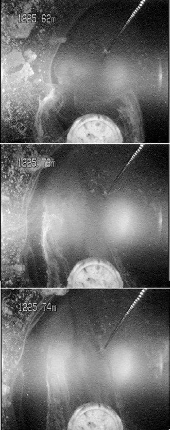
Down-looking images from the IBC deployed at 1225 m in Ice Stream C, Antarctica. A chain, as an aid to determining depth of viewing, and a compass, out of focus in this picture, are visible, as is the bore hole wall. This kind of image designed to provide data on bed nature and relative movement.

In Figure 1three frames of down-looking data are shown to illustrate the flow of water at the base of Ice Stream C taken in the 2000–01 study. The flow is visible in filaments of fine debris being advected toward the top of the image and demonstrating that the basal hydrology is active at this point. Flow is visible because the water has entrained a small amount of bed material, probably loess. If the material is in too great or too small concentration, the flow cannot be visualized with this technique, but if the water is too opaque as a result of the hot-water drill suspending it, it will clear in time if the hydrology is in fact active.

JPL Laser Dust Nephelometer

Standard digital camera images are of great value as descriptive data, and these data can be quantitatively inter­is preted for such variables as the distribution and size of large inclusions. Many other kinds of information are available using optical interrogation, and we demonstrate here that Mie scattering for dust analysis is at least as useful for in situ observations as for the well-established core analysis (Reference Ram and KoenigRam and Koenig, 1997) and that it provides data at finer resolution than some in situ strategies (Reference Bay, Price, Clow and GowBay and others, 2001). If the Mars ice is sufficiently clear that extinction lengths of several centimeters are realized, quantitative analysis of included dust can be addressed. We recognize here that Earth ice-sheet ice has very little in the way of impurities (∼0.01%), and that Mars ice may bear significantly more dust (perhaps as much as 20%).

Dust in ice sheets has long been known to vary by season and on longer terms due to climate change (Reference Hammer, Clausen, Dansgaard, Gundestrup, Johnsen and ReehHammer and others, 1978; Reference Dahl-Jensen, Thorsteinsson, Alley and ShojiDahl-Jensen and others, 1997; Reference Ram and KoenigRam and Koenig, 1997; Reference SteffensenSteffensen, 1997; Reference PetitPetit and others, 1999). For these concentrations, optical techniques are well established, first on meltwater and then on bubble-free ice itself, for assessment of the dust burden as it varies with depth and consequently time. In the bubble-free part of the core, light was scattered by dust particles (Reference Ram, Illing, Weber, Koenig and KaplanRam and others, 1995) over a dynamic range from a few to nearly 5000 relative units. Later the Greenland Ice Sheet Project 2 (GISP2) optics were calibrated (Reference Ram, Donarummo, Stolz and KoenigRam and others, 2000) to cover a range of dust loading to 4 10 000 μg kg–₁, and the signal intensity was linear with dust mass, as required for single-scattering. The results of Reference SteffensenSteffensen (1997) on meltwater and the scattering profiles of Ram and others are not suited to 1:1 comparison for several reasons, but they agree in substance. Light scattering from microbubbles associated with pressure relief long after ice-core removal was a problem for deep ice from cold intervals having high impurities (Reference Ram, Donarummo, Stolz and KoenigRam and others 2000), and is probably a source of error for this work as well. The crucial facts are that adequate climatically driven dynamic range exists, in the deep ice of Greenland, with particles suited to assessment by optical scattering, as predicted for the single-scattering regime.

Dust in the ice largely comes from three sources: ordinary atmospheric transport, dust storms and volcanic eruptions. Both Greenland Icecore Project (GRIP) and GISP2 dust analyses find the particle-size distributions close to power-law in form, with means in radius near 1 × 10_–6 m for both background dust and dust storms and for all climate conditions. A detailed and thorough analysis of the dust-storm events and the background dust in the GISP2 ice (Reference DonarummoDonarummo, 1997) shows that the size distribution is modified to somewhat larger particles, and the total dust mass is increased dramatically (in excess of an order of magnitude) during dust storms compared to background transport. The GRIP ice dust was comprehensively analyzed by Reference SteffensenSteffensen (1997) with results similar to GISP2, including a small shift of size distribution peak upward with colder climates, from about 0.9610–6 m (Holocene) to 1610–6 m (Last Glacial Maximum (LGM)). Total dust mass ranged from <50 μg kg–1 (recent) to >7000 μg kg–1 (LGM), and again the total dust mass is distributed strongly (84–99%) in the particle range centered at 1610–6 m radius. Reference PetitPetit and others (1999) examined ice from East Antarctica, and their results also show particles clustered near 1610–6 m radius, with a slight increase in size for glacial periods.

Particles near 1610–6 m radius constitute an ideal size distribution for optical measurement. Mars atmospheric dust has been optically examined and found to be in the same size range (Reference Ockert-Bell, Bell, Pollack, C. and ForgetOckert-Bell and others, 1997; Reference Tomasko, Doose, Lemmon, P. Smith and WegrynTomasko and others, 1999), as would be expected given that the deposition rate for this dust is pressure-independent. Clearly the Mars ice caps are expected to contain dust, and the dust should be in the size range for optical investigation using visible wavelength light. Theonly real issue is that of total dust-mass loading; if Mars ice has too much dust mass (or too little, which is unlikely) the single-scattering assumption will fail and the signal strength will not be readily interpretable.

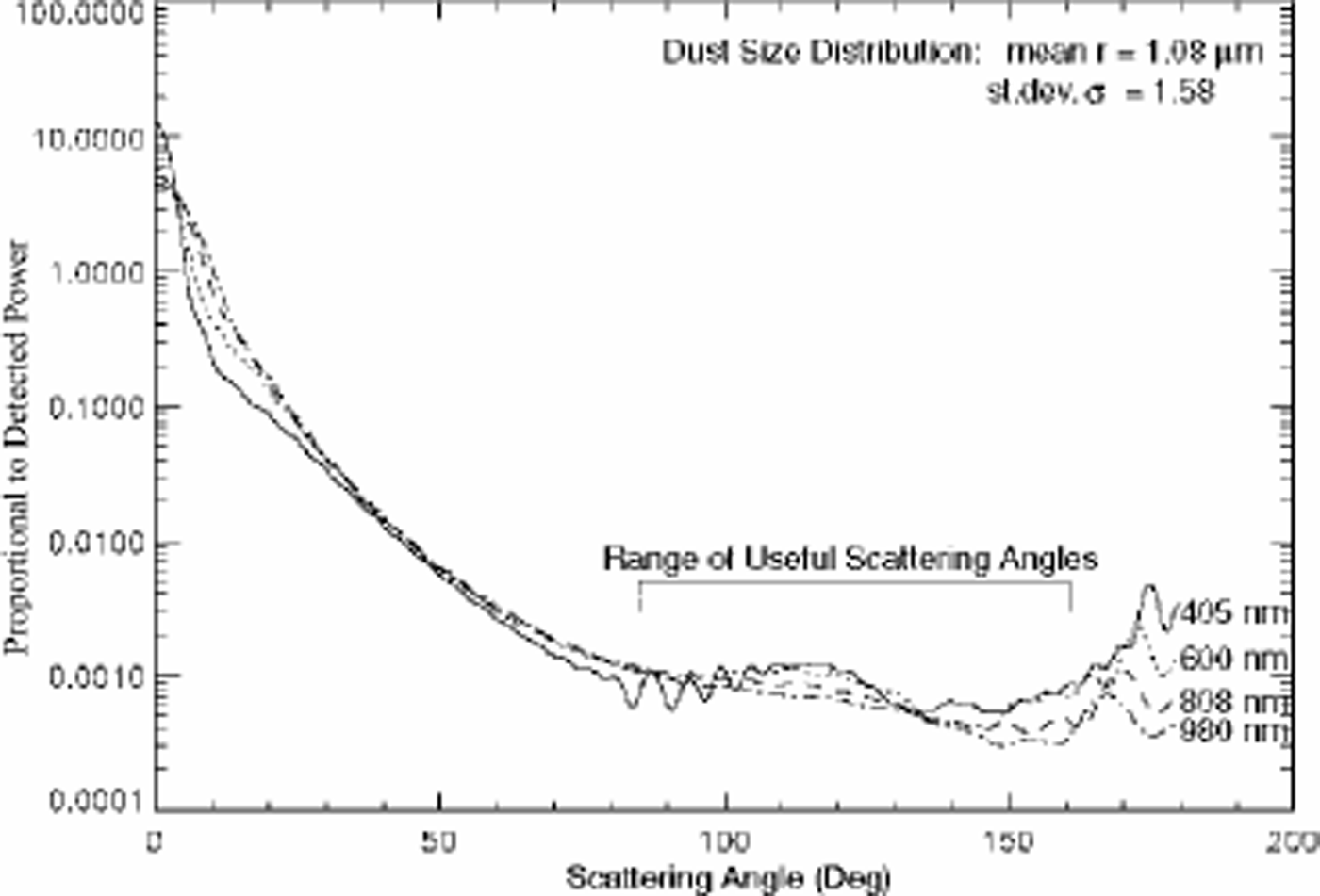
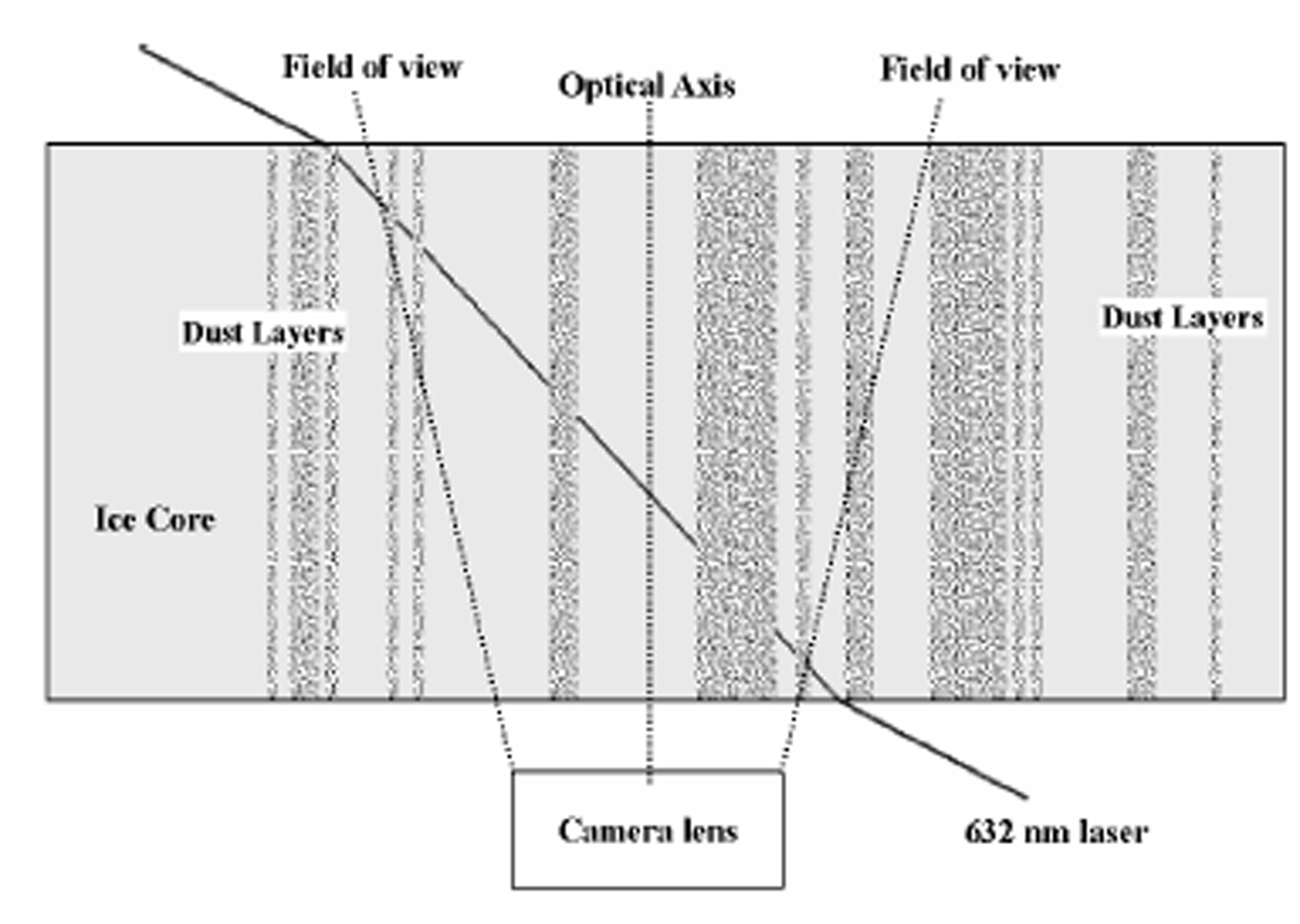
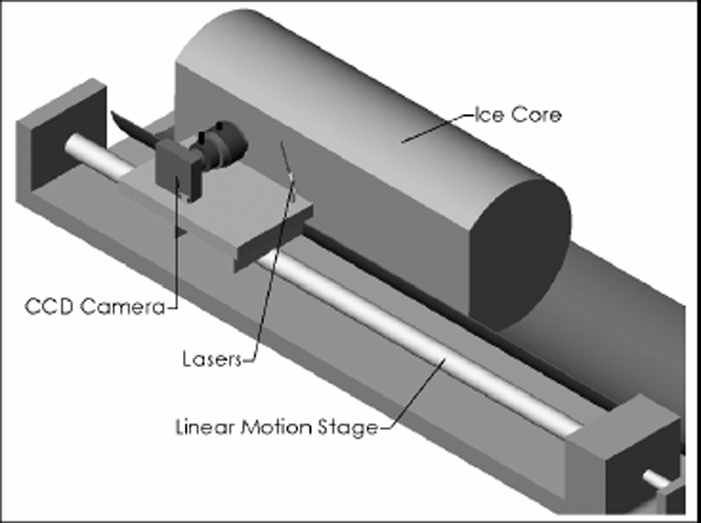
In Figure 2 we show the predicted detected power (using Reference Bohren and HuffmanBohren and Huffman, 1998) per 1000 particles, for light scattering from the Greenland distribution of dust particles (Reference SteffensenSteffensen, 1997). The flattening of the curve near 120°, and the relative insensitivity to wavelength mean that scattered light can be inverted to obtain the density of scatterers. To utilize the scattered power, the observational geometry of Figure 3 is employed. Note that the scattering angle varies from about 90° where the laser beam enters the camera field of observation on the right, and increases to about 130° where the beam exits. This geometrical set-up is accomplished with an ice core using equipment as configured in Figure 4. This geometry was used at the U.S. National Ice Core Laboratory (NICL) using an SBIG astronomical camera and solid-state red laser, and data were taken using a variety of exposure times and angles.

Fig. 2.

Predicted scattering using Mie equations for a collection of particles with the size distribution of Reference SteffensenSteffensen (1997). The geometry used obtains data over about 30° selectable from the range indicated in the plot. The use of particles in a range of sizes and shapes tends to wash out the lobes present in single-size calculations.

Fig. 3.

A cartoon of an ice core with dusty layers with oblique laser illumination and a camera to record scattered light.

Fig. 4.

As in Figure 3 except a computer-aided drawing of the observational system for using oblique laser scattering with an ice core. The core has a flat on one side as is usual for modern cores.

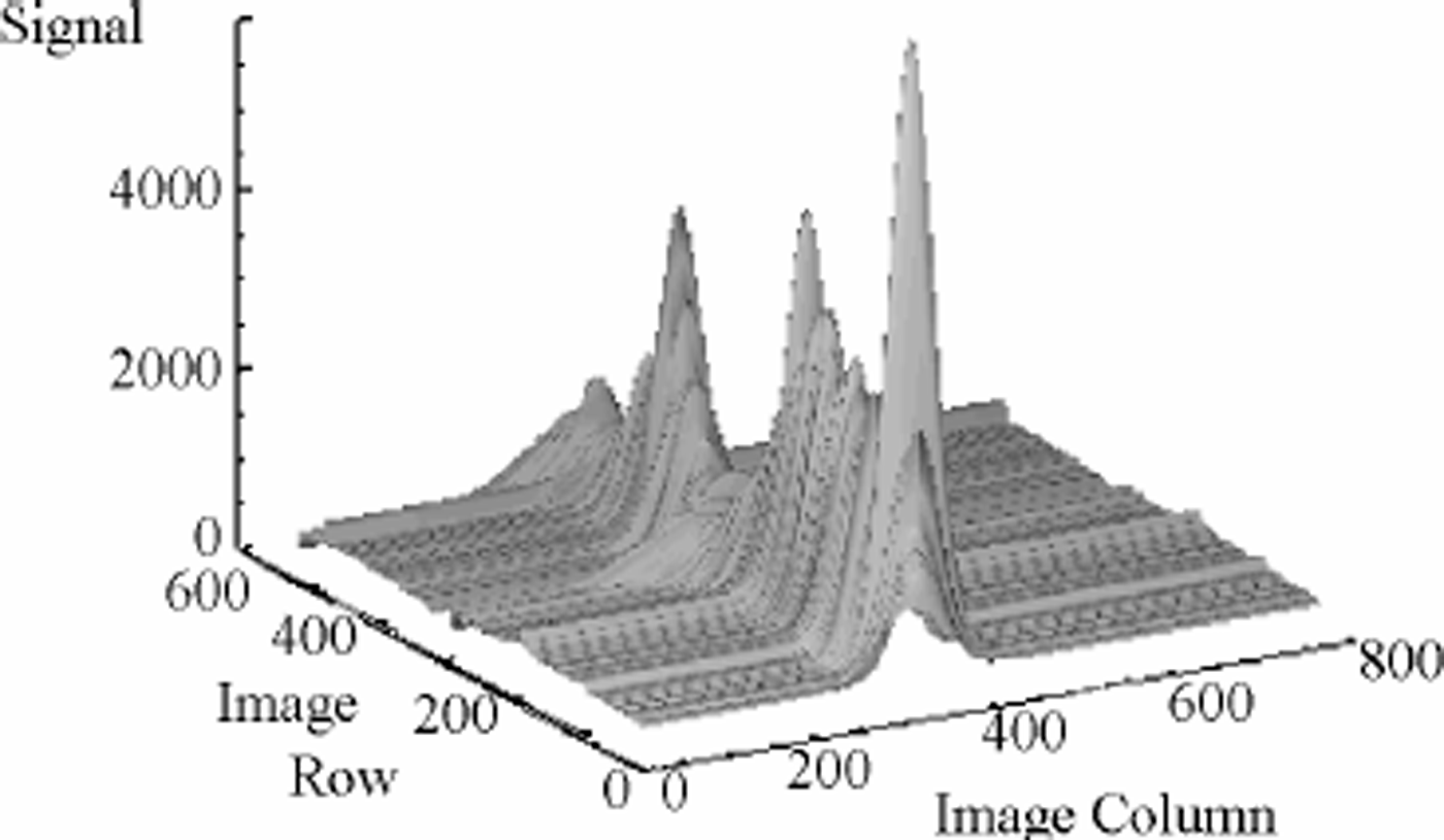
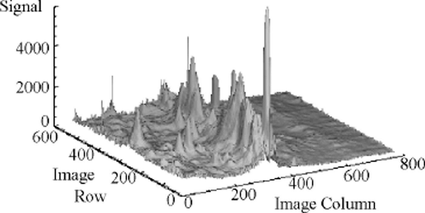
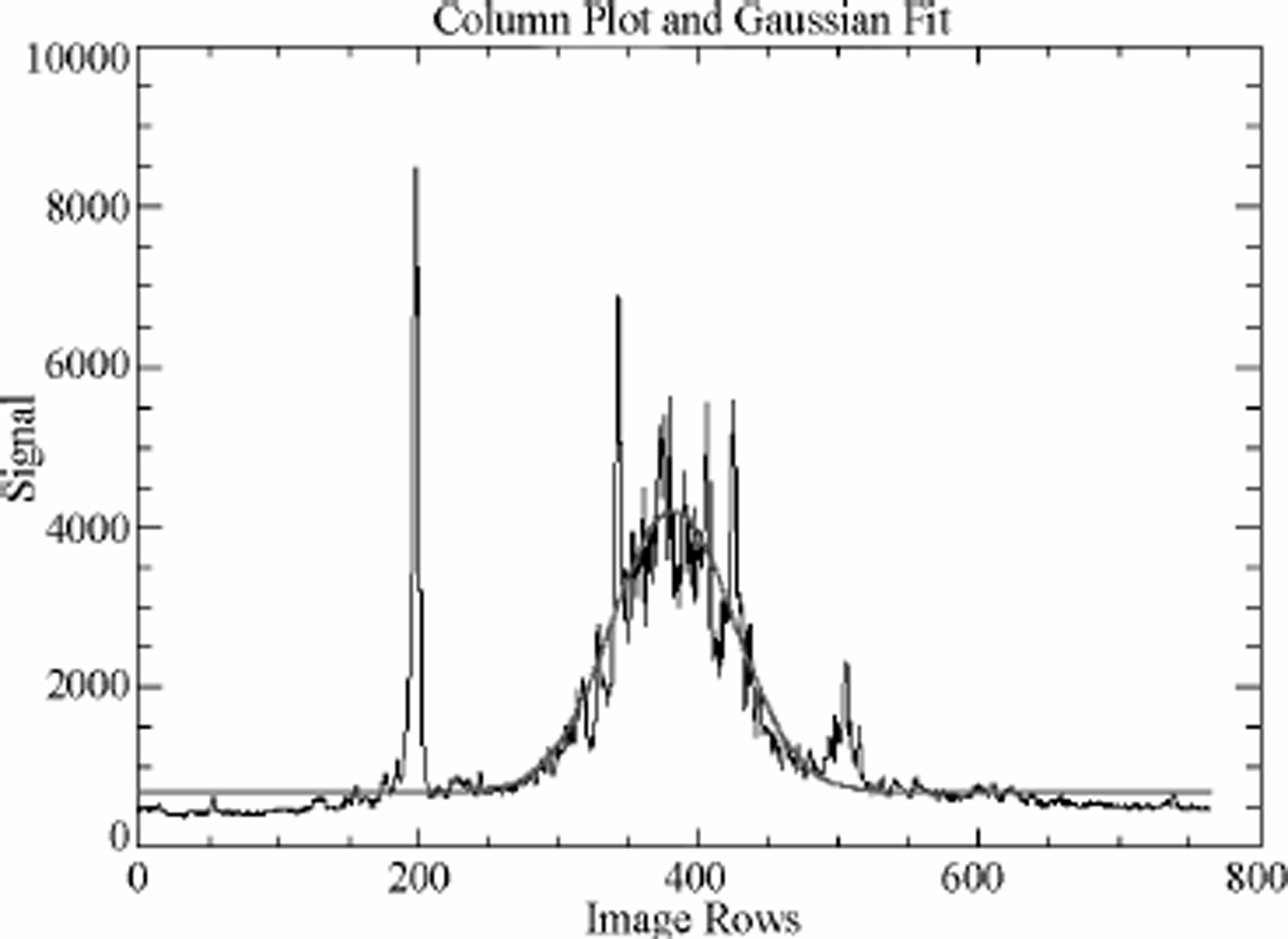
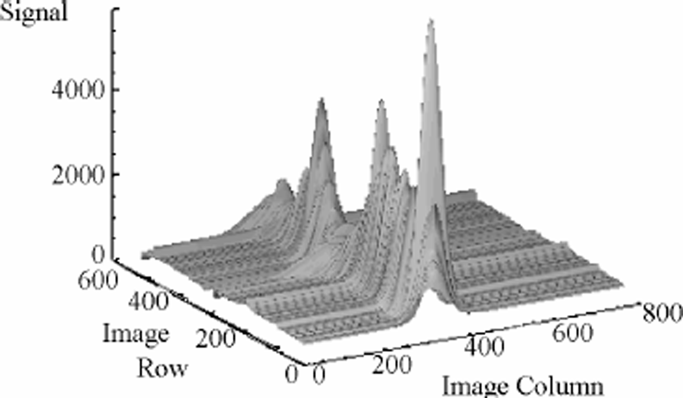
An image of data taken from 2503 m in the GISP2 core is shown in Figure 5 where the laser beam crosses the image from right to left near the center of the frame; layers of dust can clearly be seen in this negative image. Two aspects of the scattering are noteworthy. First, the less dusty levels are remarkably clear and well defined; secondly, the dusty intervals are characterized by measured light from above and below (in the figure) the center of the beam. This light is almost certainly due to multiple scattering. The image data are shown in Figure 6 in a three-dimensional format. The sharp peaks are taken to be light scattering from bubbles and other large inclusions, possibly present as a result of the 9 years that this ice has been resting at one atmosphere pressure. In Figure 7 a single row from an image is displayed along with a Gaussian fit to the curve with maximum near row 400 as this represents the path of the laser beam; each camera pixel represents 40 x 10_–6 m of ice. The laser beam is itself Gaussian. When the Gaussian smoothing is applied to the whole image, the three-dimensional representation in Figure 8 is the result. Strictly speaking, the peaks of the curves should be strongly analogous to the laser light-scattering (LLS) results of Reference Ram, Donarummo, Stolz and KoenigRam and others (2000).

Fig. 5.

A negative image taken in the geometry of Figure 4. Here the laser light is across the image from right to left, and the dark band across the center represents light scattered by dust. Other black spots are due to bubbles in the ice; they are large and very efficient scatterers of even stray light. Note the abruptness of the dusty-to-clear transition.

Fig. 6.

A three-dimensional representation of the scattering image shown in Figure 5. Note that the noise peaks off the laser track (and possibly those on the laser track as well) are narrow and can be very tall (bright).

Fig. 7.

One row from a scattering image. Here the dust data are represented by the maximum around 400 pixels, and bubble scatter noise can be seen near 200 and 500 pixels. The smooth line is a Gaussian fit to the data near pixel 400.

Fig. 8.

As in Figure 6, a three-dimensional representation of the scattering image, but this time the “data” shown are the Gaussian best fits as demonstrated in Figure 7.

In Figure 9 we show 3 cm of images with the laser dust nephelometer system compared to the Reference Ram, Donarummo, Stolz and KoenigRam and others (2000) results (as acquired from the U.S. National Snow and Ice Data Center (NSIDC)). To construct Figure 9, images were acquired on 5 mm translations of the camera laser down the core, and the separate image data are shown as different lines. Note that the image-to-image correlation is very good. In the lower graph of Figure 9, the Reference Ram, Donarummo, Stolz and KoenigRam and others (2000) data are shown; these data are archived at1mm resolution at 2500m depth. It is not possible at this time to locate precisely the laser nephelometer data with respect to the archived laser scattering data, as absolute depth could not be determined accurately due to an uneven core end, but the similarity in spatial data strongly suggests that the same dust signal is being investigated, as one would expect since the basic measurement principle is the same, only the geometry is slightly different.

Fig. 9.

(a) Gaussian area vs depth acquired by the laser nephelometer. The different lines are from different frames of the camera and laser translated 5 mm for each frame. (b) LLS data from GISP2 (Reference Ram and KoenigRam and Koenig, 1997) acquired NSIDC. We have taken the liberty of moving the Ram and Koenig data along a few centimeters to obtain an optimal core end is quite uneven, and it was not possible to tell the precise depth.

New Technology

We have described new technologies motivated primarily by their application to planetary ice observations. These technologies have, in addition, potential use in Earth Science. Ice cores are of immense value and are highly expensive. Cryobot profiles of ice sheets and caps offer the capability to acquire limited data with more extensive coverage at reduced cost to supply information relevant to such processes as paleocirculation and deformation. Cryobot profiles can also aid in the selection of sites for full coring operations.

Conclusions

We have discussed and demonstrated methods for acquiring simple but scientifically useful image data from Mars icecap ice involving a range of ice clarity from opaque ice to clear ice with banded dust inclusions analogous with Earth ice-sheet ice, although we do not expect to resolve annual layers. The detailed nature of Mars ice-cap ice is completely unknown and open to speculation for now. The general approach of optical examination can be taken considerably further of course, most notably through the use of analytical fluorescence and Raman scattering methods, which are well developed for laboratory work. It is our intention to develop these additional means of optically interrogating ice for future investigations of ice of Earth, Mars and Europa.