









1 Introduction
The rational homology of
$\operatorname {\mathrm {Out}}(F_n)$
 has been extensively studied in the last thirty years. The groups
$H_i(\operatorname {\mathrm {Out}}(F_n); \mathbb {Q})$
 have been computed for
$n \leq 7$
 and
$i \in \mathbb {Z}$
 by Vogtmann [Reference VogtmannVog06], Gerlits [Reference GerlitsGer02], Ohashi [Reference OhashiOha08], and Bartholdi [Reference BartholdiBar16]. The main tool for these calculations is the cellular structure of the spine of the Culler–Vogtmann Outer space [Reference Culler and VogtmannCV86] and its filtration due to Kontsevich [Reference KontsevichKon93, Reference KontsevichKon94, Reference Conant and VogtmannCV03].
Culler and Vogtmann [Reference Culler and VogtmannCV86] showed that the virtual cohomological dimension of
$\operatorname {\mathrm {Out}}(F_n)$
 is equal to
$2n-3$
 . Hatcher and Vogtmann proved that
$H_i(\operatorname {\mathrm {Out}}(F_n); \mathbb {Q})$
 stabilises when n is large enough [Reference Hatcher and VogtmannHV04] and Galatius showed that the stable value vanishes [Reference GalatiusGal11]. Further computations have been done towards understanding the classical rational and orbifold Euler characteristics of
$\operatorname {\mathrm {Out}}(F_n)$
 . The results of [Reference Morita, Sakasai and SuzukiMSS15, Reference Borinsky and VogtmannBV20, Reference Borinsky and VogtmannBV23] imply that in general the rational homology
$H_*(\operatorname {\mathrm {Out}}(F_n); \mathbb {Q})$
 contains many odd dimensional classes (in fact more than even dimensional classes). However, writing down these odd classes explicitly seems to be very difficult. For
$n \leq 6$
 the rational homology
$H_*(\operatorname {\mathrm {Out}}(F_n), \mathbb {Q})$
 is even (see, e.g., [Reference OhashiOha08]). A nontrivial odd dimensional group is computed in [Reference BartholdiBar16], where Bartholdi shows that
$H_{11}(\operatorname {\mathrm {Out}}(F_7); \mathbb {Q})$
 is isomorphic to
$\mathbb {Q}$
 . Bartholdi’s result uses Kontsevich’s filtration and computer calculations. No other odd dimensional nontrivial rational homology groups of
$\operatorname {\mathrm {Out}}(F_n)$
 have been detected so far.
In this paper we give a systematic way of producing odd dimensional classes in the rationalised complex topological K-theory of
$B\operatorname {\mathrm {Out}}(F_n)$
 . We show that for any prime
$p \geq 11$
 , the
$\mathbb {Q}$
 -vector space
$K^1(B\operatorname {\mathrm {Out}}(F_{p+1})) \otimes _{\mathbb {Z}} \mathbb {Q}$
 is nontrivial by providing a quadratic lower bound
$\frac {1}{24}(p-7)(p-5)$
 for the
$\mathbb {Q}_p$
 -dimension of its p-adic summand. We do not need any computer calculations to verify this. The main tools for our computations are the equivariant Chern character of Lück [Reference LückLü07] and the generalised Farrell–Tate cohomology defined by Klein in [Reference KleinKle01, Reference KleinKle02]. Before we explicitly formulate our results, we review general results on rational K-theory and Farrell–Tate cohomology.
Lück [Reference LückLü07] provided a conceptual way to compute the rational K-theory of
$BG$
 , where G is an infinite discrete group which admits a finite classifying G-space for proper actions. This classifying G-space is denoted by
$\underline {E}G$
 . It is uniquely determined up to G-equivariant homotopy equivalence by the properties that it is a G-CW complex and the fixed subspace
$\underline {E}G^H$
 is contractible if H is finite and empty otherwise. We say that G admits a finite
$\underline {E}G$
 if there is a finite G-CW complex model for
$\underline {E}G$
 . Equivalently, we can ask that the quotient
$\underline {E}G/G$
 is compact. For more details on
$\underline {E}G$
 and examples, see [Reference LückLü05b]. The following theorem of Lück is the main calculational tool in this paper [Reference LückLü07, Theorem 0.1]:
Theorem 1.1 (Lück)
Let G be a discrete group with a finite
$\underline {E}G$
 . Then for any
$m\in \mathbb {Z}$
 , the equivariant Chern character map

is an isomorphism, where
$\operatorname {\mathrm {con}}_p(G)$
 denotes the set of conjugacy classes of the nontrivial p-power-order elements, and
$C \langle g \rangle $
 denotes the centraliser of the cyclic subgroup generated by g.
For virtually torsion-free groups with finite virtual cohomological dimension and certain geometric finiteness conditions, an analogous theorem was obtained by Adem [Reference AdemAde92, Reference AdemAde93].
In this paper it will be convenient to mostly work with p-adic K-theory
$K_p$
 which sees the rational cohomology of
$BG$
 and the p-adic part of the above formula. The p-adic K-theory spectrum is defined as the p-completion of the complex K-theory spectrum [Reference BousfieldBou79, Section 2]. It follows from Lück’s formula (see also [Reference AdemAde93, Theorem 6.3]) that the Chern character induces an isomorphism for any
$m\in \mathbb {Z}$
 :

Various calculations have been done using this formula. Groups to which this formula was applied include certain graph products, arithmetic groups and mapping class groups (see, e.g., [Reference AdemAde92, Reference AdemAde93, Reference Lück, Patchkoria and SchwedeLPS24]). We list some of them: the amalgamated product
$L \ast _H M$
 , where
$H \leq L,M$
 , and
$H,L,M$
 are finite,
$\operatorname {\mathrm {SL}}_3(\mathbb {Z})$
 ,
$\operatorname {\mathrm {SL}}_2(\mathcal {O}_F)$
 , where F is a totally real field,
$\operatorname {\mathrm {SL}}_{p-1}(\mathbb {Z})$
 ,
$\operatorname {\mathrm {Sp}}_{p-1}(\mathbb {Z})$
 , for p an odd prime, the mapping class group
$\operatorname {\mathrm {MCG}}(\Sigma _{\frac {p-1}{2}})$
 , for
$p \geq 5$
 , and the right angled Coxeter group
$W(L)$
 , where L is a finite graph. (An alternative approach using a concrete cellular structure was used in [Reference Degrijse and LearyDL17] to compute the complex K-theory of
$BW(L)$
 .)
The Chern character isomorphism of Lück shows that it is more difficult to compute the rational (p-adic) K-theory of
$BG$
 than the rational cohomology of
$BG$
 since the latter is a direct factor of the former. However, one could expect that if the centralisers are not too large, then the factor

might be easier to compute. This is indeed the case for certain groups and primes as we will see below. But before we mention these computations, we give a conceptual interpretation of the latter summand in terms of Klein’s Farrell–Tate K-theory [Reference KleinKle01, Reference KleinKle02].
Let G be a virtual duality group in the sense of [Reference BrownBro82, Section VIII.11] with finite virtual cohomological dimension d. The classical Farrell–Tate cohomology groups
$\widehat {H}^*(G,M)$
 , defined in [Reference FarrellFar78] and [Reference BrownBro82], measure the failure of the duality map

being an equivalence. Here
$D_G$
 denotes the dualising module
$H^d(G; \mathbb {Z}[G])$
 and M is any
$\mathbb {Z}[G]$
 -module. If the Farrell–Tate cohomology vanishes for a general M, then G is a Bieri–Eckmann duality group [Reference Bieri and EckmannBE73]. If M is a
$\mathbb {Q}[G]$
 -module, then the Farrell–Tate cohomology groups
$\widehat {H}^*(G,M)$
 vanish, witnessing the fact that virtual duality groups are rational duality groups [Reference BieriBie81, Theorem 9.2] (see also [Reference BrownBro82, Section X.3]).
Now if we take any generalised cohomology theory
$E^*(-)$
 and a group G, following Klein [Reference KleinKle01, Reference KleinKle02], one can define the associated generalised Farrell–Tate cohomology
$\widehat {E}^*(BG)$
 with coefficients in E. These groups measure the failure of duality in E-(co)homology. In the special case
$E=K_p$
 , one obtains the p-adic Farrell–Tate K-theory groups
$\widehat {K_p}^*(BG)$
 . Before giving the technical definition of
$\widehat {K_p}^*(BG)$
 , we observe that the importance of these groups becomes clear from the following proposition which we prove as Proposition 4.1 in Section 4:
Proposition A. Let G be a discrete group with a finite
$\underline {E}G$
 and p a prime. Then for any
$m\in \mathbb {Z}$
 , the equivariant Chern character induces an isomorphism

The precise definition of the generalised Farrell–Tate cohomology is recalled in Section 3. Here we only give a sketch and compare it to the classical picture: In [Reference KleinKle01] Klein introduces a spectrum
$D_G$
 with a G-action, called the dualising spectrum. For any spectrum E with a G-action, he also constructs the norm map

going from the homotopy orbits to the homotopy fixed points [Reference KleinKle01]. The cofibre of this map is denoted by
$E^{tG}$
 and is called the generalised Farrell–Tate spectrum. These objects and constructions are direct higher homotopical generalisations of classical objects and constructions in group cohomology. The dualising spectrum
$D_G$
 is a generalisation of the dualising module
$H^d(G; \mathbb {Z}[G])$
 of a virtual duality group G with virtual cohomological dimension d. Homotopy orbits and fixed points are generalisations of (derived) G-coinvariants and G-invariants, respectively. The homotopy groups of the Farrell–Tate spectrum generalise the classical Farrell–Tate cohomology. The p-adic Farrell–Tate K-theory groups
$\widehat {K_p}^*(BG)$
 of G are then defined to be the homotopy groups
$\pi _{-\ast } (K_p^{tG})$
 , where G acts trivially on
$K_p$
 . In Section 3 we show that if G has a finite
$\underline {E}G$
 , then the groups
$\widehat {K_p}^*(BG)$
 are rational (that is, they are vector spaces over
$\mathbb {Q}$
 ).
As observed above, the Farrell–Tate K-theory measures the failure of duality in K-theory. Proposition A implies that
$\widehat {K_p}^0(BG)$
 never vanishes unless G is p-torsion-free. However,
$\widehat {K_p}^1(BG)$
 can vanish and this leads to a notion of p-adic weak duality which we introduce in Section 4. We show that
$\widehat {K_p}^1(BG)$
 vanishes if and only if the norm map

is an isomorphism. In Section 4 we give examples of groups which satisfy this weak form of duality: the arithmetic groups
$\operatorname {\mathrm {SL}}_3(\mathbb {Z})$
 ,
$\operatorname {\mathrm {Sp}}_{p-1}(\mathbb {Z})$
 , and the mapping class group
$\operatorname {\mathrm {MCG}}(\Sigma _{\frac {p-1}{2}})$
 (where
$p \geq 5$
 ). On the other hand we show that
$\operatorname {\mathrm {GL}}_{p-1}(\mathbb {Z})$
 for
$p \geq 5$
 does not satisfy this weak duality. We also show that the difference between the
$\mathbb {Q}_p$
 -dimensions of
$\widehat {K_p}^0(BG)$
 and
$\widehat {K_p}^1(BG)$
 can be arbitrarily large.
After understanding the generalities of the p-adic Farrell–Tate K-theory, we apply Proposition A to
$\operatorname {\mathrm {Out}}(F_n)$
 . In Section 7 we make a full calculation of
$\widehat {K_p}^*(B\operatorname {\mathrm {Out}}(F_n))$
 in the following cases:
-
• For $p \geq 3$
 and
$n=p-1,p$
;
-
• For $p \geq 5$
and
$n=p+1,p+2$
; -
• For $p \geq 7$
and
$n=p+3$
.


In this range
$\operatorname {\mathrm {Out}}(F_n)$
 does not contain subgroups isomorphic to
$\mathbb {Z}/p \times \mathbb {Z}/p$
 or
$\mathbb {Z}/p^2$
 and the classical Farrell–Tate cohomology is computed in [Reference Glover and MislinGM00, Reference ChenChe97]. The Farrell–Tate K-theory has not yet been explored. Chen’s thesis [Reference ChenChe97] classifies conjugacy classes of order p elements in this range excluding
$n=p+1$
 and shows that these elements are given by isometries of the rose and theta type graphs. Chen also computes the centralisers of these elements. This allows us to almost immediately compute
$\widehat {K_p}^*(B\operatorname {\mathrm {Out}}(F_n))$
 in the above range when
$n \neq p+1$
 . In particular,
$\widehat {K_p}^1(B\operatorname {\mathrm {Out}}(F_n))=0$
 unless
$n = p+1$
 . For
$n=p+3$
 , we also need a recent calculation of
$H^*(\operatorname {\mathrm {Out}}(F_3); \bigwedge ^{2} H_1(F_3;\mathbb {Q}))$
 due to Satoh [Reference SatohSat24].
The case
$n = p+1$
 requires a nontrivial geometric input. Chen’s thesis provides 3 conjugacy classes of order p elements: one given by an isometry of a rose
$R_p$
 , and the other two by isometries of theta graphs named
$\theta _{02}$
 and
$\theta _{11}$
 . All these admit obvious order p lifts to
$\operatorname {\mathrm {Aut}}(F_{p+1})$
 . We show in Section 6 that there is exactly one more conjugacy class of order p elements, represented by an element which we denote by
$\Phi $
 . This class does not admit an order p lift to
$\operatorname {\mathrm {Aut}}(F_{p+1})$
 which makes it nontrivial to study: it is induced by a rotation of the graph of Figure 1.
Figure 1

In Section 6 we classify the dimensions where such elements can occur and compute the rational homology of the centraliser of
$\Phi $
 . In order to do this, we define a map with finite kernel from
$C\langle \Phi \rangle $
 to a finite index subgroup of
$\operatorname {\mathrm {Out}}(F_2)$
 . This enables us to define an action of
$C \langle \Phi \rangle $
 on a tree (the reduced spine of
$\operatorname {\mathrm {CV}}_2$
 ). The stabilisers in this action are finite, and so a Mayer–Vietoris argument shows that the rational homology agrees with that of the quotient graph. To calculate it, we must compute the number of edge and vertex orbits, which we do by means of an equivalent computation in finite groups. The rational homology is given in Corollary 6.8. We note that the element
$\Phi $
 has also been studied in [Reference Bridson and PiwekBP24], where they show that it is the unique conjugacy class in
$\operatorname {\mathrm {Out}}(F_{p+1})$
 defining a free-by-cyclic group isomorphic to
$F_2 \times \mathbb {Z}$
 .
By combining the results of Section 6 with Proposition A, we obtain the following theorem, which we prove as Theorem 7.1 in Section 7:
Theorem B. Let
$p \geq 5$
 be a prime. Then we have

and

As a consequence, we see that when
$p \geq 11$
 , then

In particular, this produces a family of nontrivial odd dimensional classes in the K-theory of
$B\operatorname {\mathrm {Out}}(F_n)$
 . The first class occurs for
$p=11$
 , where we get

In the final section of the paper, we combine our calculations with the computations of Vogtmann, Hatcher, Brady, Gerlits, Ohashi, Bartholdi, and Satoh [Reference BradyBra93, Reference Hatcher and VogtmannHV98, Reference VogtmannVog02, Reference GerlitsGer02, Reference OhashiOha08, Reference BartholdiBar16, Reference SatohSat24]. We produce a table of low-dimensional values of
$\widehat {K_p}^*(B\operatorname {\mathrm {Out}}(F_{n}))$
 (see Table 4) and
$K_p^*(B\operatorname {\mathrm {Out}}(F_{n})) \otimes _{\mathbb {Z}} \mathbb {Q}$
 (see Table 5) which can be computed using currently available methods. For p-adic Farrell–Tate K-theory, the first odd dimensional class appears in
$\widehat {K_{7}}^1(B\operatorname {\mathrm {Out}}(F_{11}))$
 . The existence of this class requires Gerlits’ computer calculation of
$H_7(\operatorname {\mathrm {Aut}}(F_5); \mathbb {Q})$
 , which is isomorphic to
$\mathbb {Q}$
 . The next nontrivial odd class shows up in
$\widehat {K_{11}}^1(B\operatorname {\mathrm {Out}}(F_{12}))$
 , which is the class we construct explicitly using the Chern character. Further, Bartholdi’s computer calculation [Reference BartholdiBar16] implies that
$K^1(B\operatorname {\mathrm {Out}}(F_{7})) \otimes _{\mathbb {Z}} \mathbb {Q}$
 is nontrivial and the above argument shows that
$K^1(B\operatorname {\mathrm {Out}}(F_{11})) \otimes _{\mathbb {Z}} \mathbb {Q}$
 is nonzero. However, again the first nontrivial odd class in rational K-theory which we can see without computer calculations lives in
$K^1(B\operatorname {\mathrm {Out}}(F_{12})) \otimes _{\mathbb {Z}} \mathbb {Q}$
 .
2 Preliminaries from homotopy theory
We will use the language of model categories for simplifying the exposition. See, for example, [Reference QuillenQui67, Reference HoveyHov99] for the background in model categories. All the homotopy theoretic constructions in this paper can also be done with
$\infty $
 -categories.
The category of topological spaces is denoted by
$\operatorname {\mathrm {Top}}$
 . This is a model category with weak homotopy equivalences as weak equivalences and Serre fibrations as fibrations. Typical cofibrant objects are cellular complexes. In particular, any CW-complex is cofibrant.
Let G be a discrete group. We let
$\operatorname {\mathrm {Top}}_G$
 denote the category of G-spaces. This can be equipped with a projective model structure [Reference Schwede and ShipleySS00], where weak equivalences are G-equivariant maps which are underlying nonequivariant weak equivalences. Cofibrant objects are given by cell complexes with a free G-action. In particular, if X is a CW-complex with a G-action, then the projection map
$X \times EG \to X$
 is a cofibrant replacement.
We will also need the category of spectra
$\operatorname {\mathrm {Sp}}$
 . Here we can take any symmetric monoidal model category of spectra such as symmetric or orthogonal spectra equipped with the projective model structure, see, for example, [Reference Hovey, Shipley and SmithHSS00, Reference Mandell, May, Schwede and ShipleyMMSS01]. The symmetric monoidal structure on
$\operatorname {\mathrm {Sp}}$
 is given by the smash product which we denote by
$\otimes $
 . The unit of this structure is the sphere spectrum
$\mathbb {S}$
 . Tautologically, the category
$\operatorname {\mathrm {Sp}}$
 is equivalent to
$\mathbb {S}-\operatorname {\mathrm {Mod}}$
 . For nonexperts, one can think of the symmetric monoidal category of spectra as the higher homotopical algebra analog of the category of abelian groups with the tensor product. The unit
$\mathbb {S}$
 then behaves like
$\mathbb {Z}$
 , the unit of the tensor product. Given a spectrum E and an integer n, one can define the n-th (stable) homotopy group
$\pi _nE$
 as the group of homotopy classes of maps from the n-th suspension of
$\mathbb {S}$
 to E. In particular, one has
$\pi _0\mathbb {S} \cong \mathbb {Z}$
 . A spectrum E is called rational if
$\pi _nE$
 is a rational vector space for any
$n \in \mathbb {Z}$
 .
A ring spectrum (or an
$\mathbb {S}$
 -algebra) is an associative monoid in
$\operatorname {\mathrm {Sp}}$
 . The category
$\mathbb {S}-\operatorname {\mathrm {Alg}}$
 of ring spectra can be equipped with the projective model structure where fibrations and weak equivalences are those morphisms in
$\mathbb {S}-\operatorname {\mathrm {Alg}}$
 which are underlying fibrations and weak equivalences in
$\operatorname {\mathrm {Sp}}$
 , respectively. By [Reference Schwede and ShipleySS00, Theorem 4.1(3)], a cofibration of ring spectra is a cofibration of the underlying spectra if the source is cofibrant as a spectrum. For any ring spectrum R, the category of left and right modules
$R-\operatorname {\mathrm {Mod}}$
 and
$\operatorname {\mathrm {Mod}}-R$
 can also be equipped with projective model structures where fibrations and weak equivalences are given by the underlying notions on spectra [Reference Schwede and ShipleySS00].
The categories of spaces and spectra are related by an adjunction. The suspension spectrum functor

is a left adjoint functor which is a left Quillen functor (here
$+$
 stands for adding a disjoint basepoint). In particular, it preserves cofibrations and weak equivalences between CW-complexes.
Given a discrete group G, the suspension spectrum
$\Sigma ^{\infty }_+G$
 of the discrete space G becomes a ring spectrum using the multiplication of G. We denote this ring spectrum by
$\mathbb {S}[G]$
 . One can think of
$\mathbb {S}[G]$
 as the higher algebra analog of the group ring
$\mathbb {Z}[G]$
 . In particular, we have
$\pi _0\mathbb {S}[G] \cong \mathbb {Z}[G]$
 .
The category of abelian groups with a left (right) G-action is equivalent to the category of left (right) modules over
$\mathbb {Z}[G]$
 . Analogously, the category of G-objects in
$\operatorname {\mathrm {Sp}}$
 is equivalent to the module category
$\mathbb {S}[G]-\operatorname {\mathrm {Mod}}$
 . This is equipped with the standard model structure from [Reference Schwede and ShipleySS00] as discussed above. The suspension spectrum extends to a left Quillen functor on the level of G-objects

In particular, if X is a CW-complex with a G-action, then
$\Sigma ^{\infty }_+(EG \times X)$
 is a cofibrant replacement of
$\Sigma ^{\infty }_+X$
 . An object in
$\mathbb {S}[G]-\operatorname {\mathrm {Mod}}$
 will be called a G-spectrum for short.
Let
$H \leq G$
 be a subgroup. The the restriction functor

is a right Quillen functor whose left adjoint is given by the induction functor

These functors are analogs of the classical restriction and induction functors between
$\mathbb {Z}[G]$
 -modules and
$\mathbb {Z}[H]$
 -modules.
We will also need the mapping spectrum functor which is the analogue of the
$\operatorname {\mathrm {Hom}}$
 functor in abelian groups. The smash product
$\otimes $
 in
$\operatorname {\mathrm {Sp}}$
 has a right adjoint, the internal mapping spectrum functor
$\operatorname {\mathrm {Map}}(-,-)$
 . This functor can be used to define the generalised cohomology theory associated to any spectrum. Given a (fibrant or equivalently omega) spectrum E and a CW-complex X, the n-th E-cohomology group of X, denoted by
$E^n(X)$
 , is defined to be
$\pi _{-n}\operatorname {\mathrm {Map}}(\Sigma ^{\infty }_+ X, E)$
 .
If E and
$E'$
 are G-spectra, then
$\operatorname {\mathrm {Map}}_G(E,E')$
 denotes the mapping spectrum of G-equivariant maps. This is the fixed point spectrum of the mapping spectrum
$\operatorname {\mathrm {Map}}(E,E') \in \mathbb {S}[G]-\operatorname {\mathrm {Mod}}$
 where the action is given via the conjugation.
Finally, we will crucially use the orbit and fixed point functors. The inflation functor

which equips any spectrum with a trivial G-action has both left and right adjoints. The right adjoint sends a G-spectrum E to the fixed point spectrum
$E^G$
 and the left adjoint to the orbit spectrum
$E_G$
 . These functors are not always homotopically well-behaved, though: they are not homotopy invariant on underlying fibrant and cofibrant objects respectively. Because of this one introduces homotopy invariant versions: the homotopy fixed points
$E^{hG}$
 of E is defined to be the spectrum
$\operatorname {\mathrm {Map}}_G(\Sigma ^{\infty }_{+}EG,E)$
 . This functor preserves weak equivalences between underlying fibrant objects. Similarly the homotopy orbits
$E_{hG}$
 is defined to be the orbit spectrum
$(E \otimes \Sigma _+^{\infty }EG)_G$
 . It sends weak equivalences between underlying cofibrant objects to weak equivalences. In particular, the action on E does not have to be free for invariance of homotopy orbits. Again these definitions are motivated by the analogous notions in
$\mathbb {Z}[G]$
 -modules, namely G-invariants and G-coinvariants. In what follows we will write
$E^{hG}$
 and
$E_{hG}$
 for not necessarily underlying fibrant and cofibrant E implicitly replacing E if necessary.
3 Klein’s dualising complex and the norm map
In [Reference KleinKle01] Klein introduced a G-spectrum
$D_G$
 called the dualising spectrum and the norm map

where E is any G-spectrum. In this section we recall Klein’s construction and prove the following:
Proposition 3.1. Let G be a discrete group with a finite
$\underline {E}G$
 . Suppose E is a ring spectrum which is underlying cofibrant and let
$h \colon \mathbb {S}[G] \to E$
 be a morphism of ring spectra. If for any finite subgroup
$H \leq G$
 , the norm map

is an equivalence, then the norm map

is an equivalence.
We offer here a somewhat alternative description of the norm map in the special case when E is a ring spectrum and the G-action on the underlying spectrum of E comes from a ring spectrum map
$h \colon \mathbb {S}[G] \to E$
 . This is motivated by the following simple algebraic observation: suppose G is a finite group, R is a ring and we are given a ring homomorphism
$h \colon \mathbb {Z}[G] \to R$
 . We equip the underlying abelian group of R with a left G-action via h. Then the group
$R^G$
 of G-invariants is a right R-module via the multiplication of R from the right and hence the fixed point map
$h^G \colon \mathbb {Z}[G]^G \to R^G$
 can be extended to a map

Composing with the isomorphism
$\mathbb {Z} \cong \mathbb {Z}[G]^G$
 sending
$1$
 to the norm element
$\sum _{g \in G} g \in \mathbb {Z}[G]$
 , one recovers the norm map
$N \colon R \to R^G$
 which then factors over the G-coinvariants
$R_G$
 .
Now we start with the setup of Proposition 3.1. We use the fibrant replacement functor
$(-)^f$
 on the category of ring spectra
$\mathbb {S}-\operatorname {\mathrm {Alg}}$
 , which comes with an acyclic cofibration
$E \to E^f$
 . If E is cofibrant as a spectrum, then by [Reference Schwede and ShipleySS00, Theorem 4.1(3)], the map
$E \to E^f$
 is a cofibration of spectra. This implies that
$E^f$
 has a cofibrant underlying spectrum too.
Definition 3.2 [Reference KleinKle01]
Let G be a discrete group. Klein’s dualising spectrum
$D_G$
 is defined to be the homotopy fixed points spectrum

This spectrum is equipped with a right G-action via the right G-action on
$\mathbb {S}[G]^f$
 .
In particular, if H is a finite group, by [Reference KleinKle01, Theorem 10.1], the dualising spectrum is H-equivariantly equivalent to the sphere spectrum
$\mathbb {S}$
 with the trivial action and Klein’s norm map

specialises to the norm map

By [Reference KleinKle01, Corollary 10.2], this map is an equivalence for H-spectra of the form
$\mathbb {S}[H] \otimes Y$
 , where Y is any H-spectrum.
Let X be a finite proper G-CW complex. The morphism of ring spectra

induces a morphism on mapping spectra

The target of this morphism is a right
$E^f$
 -module using the multiplication of
$E^f$
 from the right. Hence
$h_*^f$
 induces a map

where
$EG$
 gets projected down to the base-point. Analogously to the homotopy fixed points of
$\mathbb {S}[G]$
 , the spectrum
$\operatorname {\mathrm {Map}}_G(\Sigma ^{\infty }_+(EG \times X), \mathbb {S}[G]^f)$
 has a right G-action induced by the right G-action on
$\mathbb {S}[G]^f$
 . It is now straightforward to check that the map
$\overline {N}$
 factors through G-coinvariants yielding the norm map

It follows directly from the construction in [Reference KleinKle01, Section 3] that if we take
$X=\underline {E}G$
 , then the map
$N_G$
 coincides with Klein’s norm map.
Proof of Proposition 3.1. We will show that the map

is an equivalence for any finite proper G-CW complex X. Taking
$X=\underline {E}G$
 then will yield the statement of Proposition 3.1. The map
$N_G$
 is natural in X and the source and target of
$N_G$
 send finite homotopy colimits to finite homotopy limits. Hence to show that
$N_G$
 is an equivalence, it suffices to show that it is an equivalence for
$X=G/H$
 , where
$H \leq G$
 is any finite subgroup. By the restriction-induction adjunction the map

is equivalent to the map

This map fits into a commutative diagram

where the left vertical map is induced by the inclusion
$\iota ^H \colon \mathbb {S}[H] \to \mathbb {S}[G]$
 and the diagonal map is Klein’s norm for the finite subgroup H. Hence to show that
$N_G$
 is an equivalence it suffices to show that
$\iota _*^H$
 is an equivalence. By [Reference KleinKle01, Corollary 10.2] and naturality of the norm,
$\iota _*^H$
 is equivalent to the map

induced by the inclusion
$H \leq G$
 . By definition of homotopy orbits this map is equivalent to the identity

which completes the proof.
The following is due to Klein [Reference KleinKle01]:
Definition 3.3. The Farrell–Tate spectrum of G with coefficients in E is the cofibre of the norm map and is denoted by
$E^{tG}$
 .
The homotopy groups
$\pi _{-\ast }(E^{tG})$
 can be thought as the Farrell–Tate cohomology groups with coefficients in E. In what follows we denote
$\pi _{-\ast }(E^{tG})$
 by
$\widehat {E}^*(BG)$
 .
By definition, we have a cofibre sequence

Hence the norm is an equivalence if and only if the Farrell–Tate spectrum vanishes.
Example 3.4. Suppose that we are given G, E, and
$h \colon \mathbb {S}[G] \to E$
 as in Proposition 3.1. Assume additionally that E is rational. Then the Farrell–Tate spectrum
$E^{tG}$
 vanishes. Indeed, this follows from Proposition 3.1 and from the following two facts: Finite groups are rationally acyclic and the classical norm map from coinvariants to invariants is a rational isomorphism for finite groups.
Now let
$K_p$
 denote the p-adic complex K-theory spectrum which is a (cofibrant) ring spectrum. The augmentation
$\mathbb {S}[G] \to \mathbb {S}$
 composed with the unit
$\mathbb {S} \to K_p$
 gives a map of ring spectra
$\mathbb {S}[G] \to K_p$
 which equips
$K_p$
 with the trivial G-action.
Proposition 3.5. Let G be a discrete group with finite
$\underline {E}G$
 . Then the Farrell–Tate spectrum
$K_p^{tG}$
 is rational.
Proof. Since
$K_p^{tG}$
 is p-local, it suffices to show that the mod p reduction
$(K_p/p)^{tG}$
 vanishes. By the Adams splitting we have

where
$K(1)$
 is the first Morava K-theory ring spectrum at the prime p. Again the unit precomposed with the augmentation gives a morphism of ring spectra

which equips
$K(1)$
 with the trivial G-action. Since the norm map is natural, it further suffices to show that
$K(1)^{tG}$
 vanishes. This now follows from Proposition 3.1 and a result of Greenlees-Sadofsky [Reference Greenlees and SadofskyGS96] which says that
$K(1)^{tH}$
 vanishes for H a finite group.
Remark 3.6. Let
$K(n)$
 denote the n-th Morava K-theory at the prime p. A forthcoming paper joint with Gijs Heuts will show that for any discrete group G with a finite
$\underline {E}G$
 and a
$K(n)$
 -local spectrum E with a G-action, the Farrell–Tate spectrum
$E^{tG}$
 vanishes
$K(n)$
 -locally. (See also [Reference Carmeli, Cnossen, Ramzi and YanovskiCCRY25] for a more general result on Tate vanishing.) We will also give an alternative construction of
$D_G$
 in terms of the
$\infty $
 -category of proper G-spectra of [Reference Degrijse, Hausmann, Luck, Patchkoria and SchwedeDHL+23] and [Reference Linskens, Nardin and PolLNP24] and give an
$\infty $
 -categorical proof of a more general version of Proposition 3.1 which does not require E to be a ring spectrum. We do not need these generalisations in the present paper though.
4 Farrell–Tate K-theory and duality in complex K-theory
In this section we give an explicit formula for the p-adic Farrell–Tate K-theory using Lück’s Chern character. We will also explain how exactly Farrell–Tate K-theory measures failure of duality in K-theory.
Proposition 4.1. Let G be a discrete group with a finite
$\underline {E}G$
 and p a prime. Then for any
$m \in \mathbb {Z}$
 , the equivariant Chern character induces an isomorphism

Proof. Let
$K_{\mathbb {Q}_p}$
 denote the rationalisation of the p-adic K-theory spectrum
$K_p$
 . The Farrell–Tate spectrum
$K_p^{tG}$
 is rational by Proposition 3.5. By naturality of the norm map [Reference KleinKle01], we have a commutative diagram of spectra with exact rows in the stable homotopy category:

The left vertical map is an equivalence since the rationalisation commutes with (homotopy) colimits. Hence the construction and naturality of the Chern character [Reference LückLü05a] and Theorem 1.1 imply that it suffices to show that the left lower map is an equivalence. This follows from Example 3.4.
Example 4.2. If G is a finite group, then all the centralisers are finite and hence rationally acyclic. We recover a well-known computation of the Tate construction for equivariant K-theory for finite groups (see, e.g., [Reference Jackowski and OliverJO96, page 125] and [Reference Greenlees and MayGM95, Theorem 13.1]):

and

for any integer
$m \in \mathbb {Z}$
 .
Klein has observed [Reference KleinKle01], that the Farrell–Tate spectrum
$E^{tG}$
 sees the failure of (Poincaré) duality in E-theory. Since topological K-theory is
$2$
 -periodic, Proposition 4.1 allows us to measure exactly how significant this failure of duality is. In fact, in certain cases we have some weak forms of duality.
For convenience we denote the homotopy groups
$\pi _*(D_G \otimes _{hG} K_p)$
 of the homotopy orbit spectrum by
$(K_p)_*(BG; D_G)$
 . One can think of these groups as the p-adic K-homology groups with coefficients in the local coefficient system determined by
$D_G$
 . Then by definition and Bott periodicity, we have a six-term exact sequence

In particular, we see from this long exact sequence that the rationalised norm map

is never an isomorphism of graded
$\mathbb {Q}$
 -vector spaces unless the group G is p-power torsion-free. Indeed by Proposition 4.1, the group
$\widehat {K_p}^0(BG)$
 always contains the product
$\prod _{[g] \in \operatorname {\mathrm {con}}_{p}(G)} \mathbb {Q}_p$
 as a retract.
Definition 4.3. Let G be a discrete group with a finite
$\underline {E}G$
 and p a prime. We say that G satisfies weak duality in p-adic K-theory if the map

is injective and the map

is surjective.
Proposition 4.4. Let G be a discrete group with a finite
$\underline {E}G$
 and p a prime. Then the following are equivalent:
-
(i) The group G satisfies weak duality in p-adic K-theory;
-
(ii) The p-adic Farrell–Tate K-theory group $\widehat {K_p}^1(BG)$
vanishes; -
(iii) The map
$$\begin{align*}N_G \otimes_{\mathbb{Z}} \mathbb{Q} \colon (K_p)_{-1}(BG; D_G) \otimes_{\mathbb{Z}} \mathbb{Q} \to K_p^1(BG) \otimes_{\mathbb{Z}} \mathbb{Q} \end{align*}$$
is an isomorphism.
-
(iv) For any p-power order element $g \in G$
, the centraliser
$C\langle g \rangle $
has even rational cohomology.


Proof. The equivalence
$(i) \Longleftrightarrow (ii)$
 is an easy consequence of the six term exact sequence. The equivalence
$(ii) \Longleftrightarrow (iii)$
 follows from the construction of the Chern character [Reference LückLü07], Proposition 3.5, and Proposition 4.1 which imply that the map

is split surjective. The equivalence
$(iv) \Longleftrightarrow (ii)$
 follows from Proposition 4.1.
Remark 4.5. Proposition 4.4 motivates more careful study of the rational cohomology of the centralisers
$C\langle g \rangle $
 , where g is a p-power order element. In particular, detecting nontrivial odd dimensional cohomology classes for the centralisers would automatically imply that
$\widehat {K_p}^1(BG)$
 does not vanish and hence the group G does not have weak duality in p-adic K-theory. We also note that any nontrivial odd dimensional class in
$\widehat {K_p}^1(BG)$
 gives a nontrivial odd dimensional class in the rational K-theory
$K^*(BG) \otimes _{\mathbb {Z}} \mathbb {Q}$
 which does not come from the rational cohomology. Below we will detect these kinds of odd dimensional classes in
$K^*(B\operatorname {\mathrm {Out}}(F_{p+1})) \otimes _{\mathbb {Z}} \mathbb {Q}$
 when
$p \geq 11$
 . For example, we will construct a class in
$K^1(B\operatorname {\mathrm {Out}}(F_{12})) \otimes _{\mathbb {Z}} \mathbb {Q}$
 which does not come from
$H^*(\operatorname {\mathrm {Out}}(F_{12}); \mathbb {Q})$
 .
When G satisfies weak duality in p-adic K-theory, that is,
$\widehat {K_p}^1(BG)=0$
 , then
$\widehat {K_p}^0(BG)$
 measures the exact failure of honest duality. The smaller this is, the closer to honest duality we get. By the
$6$
 -term exact sequence, the cokernel of
$N_G \colon (K_p)_0(BG; D_G) \to K_p^0(BG)$
 injects into
$\widehat {K_p}^0(BG)$
 and
$\widehat {K_p}^0(BG)$
 surjects onto the kernel of
$N_G \colon (K_p)_{-1}(BG; D_G) \to K_p^1(BG)$
 . The best possible case is when all centralisers of p-power order elements are rationally acyclic. In this case
$\widehat {K_p}^0(BG) \cong \prod _{[g] \in \operatorname {\mathrm {con}}_{p}(G)} \mathbb {Q}_p$
 .
5 Examples
In this section we compute some examples and study the behavior of their p-adic Farrell–Tate K-theory. In general all possibilities can occur: all centralisers can be rationally acyclic,
$\widehat {K_p}^*(BG)$
 can be even while some centralisers are not rationally acyclic,
$\widehat {K_p}^1(BG)$
 might not be trivial and the Farrell–Tate K-theory Euler characteristic

can be arbitrarily small or large. Simple examples can be provided by direct products
$G \times \mathbb {Z}/p$
 , where G is a p-torsion free group with a finite
$\underline {E}G$
 . For instance we could take the following examples to cover some of these cases:
$G=F_n$
 and p any prime,
$G=\operatorname {\mathrm {Sp}}_4(\mathbb {Z})$
 and
$p \geq 7$
 ,
$G=\operatorname {\mathrm {SL}}_4(\mathbb {Z})$
 and
$p \geq 7$
 , and
$G=\operatorname {\mathrm {SL}}_2(\mathbb {Z})$
 and
$p=5$
 . We do not go into details of these examples because they are straightforward. All these examples have central order p elements and hence centralisers are very large (in fact the full group). Our goal below is to provide interesting examples where centralisers are quite small, showing the usefulness of Proposition 4.1.
We start with arithmetic groups. It follows from [Reference JiJi07] that any arithmetic group admits a finite
$\underline {E}G$
 .
5.1 The general linear group
$\operatorname {\mathrm {SL}}_3(\mathbb {Z})$

The group
$\operatorname {\mathrm {SL}}_3(\mathbb {Z})$
 has only
$2$
 and
$3$
 -primary torsion. The K-theory of
$B\operatorname {\mathrm {SL}}_3(\mathbb {Z})$
 is computed in [Reference Tezuka and YagitaTY92] and is shown to be even. Soulé in [Reference SouléSou78] provided a finite cellular model of
$\underline {E}\operatorname {\mathrm {SL}}_3(\mathbb {Z})$
 and showed that
$\underline {E}\operatorname {\mathrm {SL}}_3(\mathbb {Z})/\operatorname {\mathrm {SL}}_3(\mathbb {Z})$
 is contractible. Hence,
$\operatorname {\mathrm {SL}}_3(\mathbb {Z})$
 is in particular rationally acyclic. The papers [Reference AdemAde92] and [Reference Lück, Patchkoria and SchwedeLPS24] show that the centralisers of prime power order elements are rationally acyclic. This implies that for any prime p, we have

and hence
$\operatorname {\mathrm {SL}}_3(\mathbb {Z})$
 satisfies weak duality in p-adic K-theory. By [Reference Tezuka and YagitaTY92] and [Reference TaharaTah71], we know the classification of finite order elements: there are
$2$
 conjugacy classes of order
$3$
 elements,
$2$
 conjugacy classes of order
$2$
 elements and
$2$
 conjugacy classes of order
$4$
 elements. Hence

and

5.2 The general linear group
$\operatorname {\mathrm {GL}}_{p-1}(\mathbb {Z})$
for a prime
$p \geq 5$


It follows from [Reference AshAsh89, Section 2] and [Reference Levitt and NicolasLN98] that any nontrivial p-subgroup of
$\operatorname {\mathrm {GL}}_{p-1}(\mathbb {Z})$
 is isomorphic to
$\mathbb {Z}/p$
 . Further, the paper [Reference Latimer and MacDuffeeLM33] (see also [Reference Sjerve and YangSY97, Reference AshAsh89]) implies that the conjugacy classes of order p elements are in bijection with the ideal class group
$\operatorname {\mathrm {Cl}}(\mathbb {Q}(\zeta _p))$
 . It follows from [Reference AshAsh89, Lemma 4] that
$C\langle A \rangle $
 for any A of order p is isomorphic to the group of units in
$\mathbb {Z}[\zeta _p]$
 which, by the Dirichlet unit theorem, is isomorphic to

Hence by Proposition 4.1, we get

and

These formulas combined with Lück’s theorem (Theorem 1.1) recover a calculation of Adem ([Reference AdemAde93, Example 6.7] and [Reference AdemAde92, Example 4.5]). We see that the group
$\operatorname {\mathrm {GL}}_{p-1}(\mathbb {Z})$
 does not satisfy weak duality in p-adic K-theory and the Farrell–Tate K-theory Euler characteristic vanishes.
5.3 The symplectic group
$\operatorname {\mathrm {Sp}}_{p-1}(\mathbb {Z})$
for a prime
$p \geq 5$


It follows from [Reference AshAsh89, Section 2] and [Reference Levitt and NicolasLN98] that any nontrivial p-subgroup of
$\operatorname {\mathrm {Sp}}_{p-1}(\mathbb {Z})$
 is isomorphic to
$\mathbb {Z}/p$
 . The paper [Reference Sjerve and YangSY97] shows that the conjugacy classes of the elements of order p in
$\operatorname {\mathrm {Sp}}_{p-1}(\mathbb {Z})$
 are in bijection with the set of equivalence classes of the pairs
$(I, a)$
 , where I is an integral ideal in
$\mathbb {Z}[\zeta _p]$
 and
$I \cdot \overline {I}=(a)$
 , where
$a=\overline {a}$
 . It follows form [Reference Sjerve and YangSY97, Theorem 3] that the number of such equivalence classes is equal to
$2^{\frac {p-1}{2}}h_p^{-}$
 , where

is the relative class number. By [Reference BuschBus02, Section 3.2] and [Reference BrownBro74], we know that for any element A of order p, the centraliser of A is finite and

As a consequence by Proposition 4.1, we get

and

In particular,
$\operatorname {\mathrm {Sp}}_{p-1}(\mathbb {Z})$
 satisfies weak duality in p-adic K-theory.
5.4 The mapping class group
$\operatorname {\mathrm {MCG}}(\Sigma _{\frac {p-1}{2}})$
for a prime
$p \geq 5$


Let
$\operatorname {\mathrm {MCG}}(\Sigma _{\frac {p-1}{2}})$
 be the mapping class group of the closed oriented surface of genus
$\frac {p-1}{2}$
 . The papers [Reference BroughtonBro90, Reference Ji and WolpertJW10, Reference MislinMis10] show that mapping class groups admit a finite model for
$\underline {E}G$
 .
It follows from [Reference XiaXia90, Chapter III] that any nontrivial finite p-subgroup of
$\operatorname {\mathrm {MCG}}(\Sigma _{\frac {p-1}{2}})$
 is isomorphic to
$\mathbb {Z}/p$
 . By [Reference XiaXia90, Section 3.1], the number of conjugacy classes of order p elements is equal to

Additionally it follows from [Reference XiaXia90, Section 3.2] that the centralisers of order p elements are finite. Hence, by Proposition 4.1

and

In particular,
$\operatorname {\mathrm {MCG}}(\Sigma _{\frac {p-1}{2}})$
 satisfies weak duality in p-adic K-theory.
5.5 Amalgamated products of finite groups
Interesting examples arise by considering amalgamated products of finite groups. By Bass–Serre theory [Reference SerreSer03], we know that any such group admits a finite
$\underline {E}G$
 , its Bass–Serre covering tree. Consider

where p is an odd prime and
$\mathbb {Z}/(p-1)$
 is acting as the automorphism group of
$\mathbb {Z}/p$
 . Then G has only one conjugacy class of order p elements and its centraliser is isomorphic to

where
$F_{p-2}$
 is the free group on
$p-2$
 generators. By Proposition 4.1, we get

and

This group does not satisfy weak duality in p-adic K-theory. The Farrell–Tate K-theory Euler characteristic is equal to
$3-p$
 and goes to
$-\infty $
 when the prime increases. We note though that the group G is rationally acyclic.
To summarise, we saw that the groups
$\operatorname {\mathrm {SL}}_3(\mathbb {Z})$
 ,
$\operatorname {\mathrm {Sp}}_{p-1}(\mathbb {Z})$
 ,
$\operatorname {\mathrm {MCG}}(\Sigma _{\frac {p-1}{2}})$
 satisfy weak duality, while
$\widehat {K_p}^0(BG)$
 can be an arbitrarily large finite dimensional
$\mathbb {Q}_p$
 -vector space. The group
$\operatorname {\mathrm {GL}}_{p-1}(\mathbb {Z})$
 provides an example where
$\widehat {K_p}^0(BG)$
 and
$\widehat {K_p}^1(BG)$
 have the same dimension (increasing with p) and hence the Farrell–Tate K-theory Euler characteristic vanishes. Aside from
$\operatorname {\mathrm {SL}}_3(\mathbb {Z})$
 which is rationally acyclic by [Reference SouléSou78], the rational cohomologies of these groups are not fully computed. The last example shows that
$\widehat {K_p}^1(BG)$
 can be arbitrarily large while
$\widehat {K_p}^0(BG)$
 is as small as possible and G is rationally acyclic. Below we will show that
$\operatorname {\mathrm {Out}}(F_{p+1})$
 provides a similar example to the latter but in this case the rational cohomology is very interesting and far away from being computed.
6 Elements of order p and their centralisers
In this section we study conjugacy classes of order p elements in
$\operatorname {\mathrm {Out}}(F_n)$
 when
$p-1 \leq n \leq 2p-3$
 and their centralisers. The results when
$n \neq p+1$
 are well known and can be found in [Reference ChenChe97, Reference Glover, Mislin and VoonGMV98]. By [Reference Glover, Mislin and VoonGMV98, Corollary 2.2] the group
$\operatorname {\mathrm {Out}}(F_n)$
 is p-periodic for
$p-1 \leq n \leq 2p-3$
 , that is, it does not contain
$\mathbb {Z}/p \times \mathbb {Z}/p$
 as a subgroup. Additionally, the natural map
$\operatorname {\mathrm {Out}}(F_n) \to \operatorname {\mathrm {GL}}_n(\mathbb {Z})$
 has torsion-free kernel and there are no order
$p^2$
 elements in
$\operatorname {\mathrm {GL}}_n(\mathbb {Z})$
 in this range [Reference Levitt and NicolasLN98]. Hence any finite p-subgroup of
$\operatorname {\mathrm {Out}}(F_n)$
 for
$p-1 \leq n \leq 2p-3$
 is isomorphic to
$\mathbb {Z}/p$
 .
All the graphs we consider in this section are connected. We establish the following conventions for our actions. (Note that as soon as one of these is decided, the others follow.)
-
(1) $F_n$
acts on trees on the left; -
(2) $\operatorname {\mathrm {Aut}}(F_n)$
acts on
$F_n$
on the left; -
(3) $\operatorname {\mathrm {Aut}}(F_n)$
(hence
$\operatorname {\mathrm {Out}}(F_n)$
) acts on
$\operatorname {\mathrm {CV}}_n$
on the right.


We need the following theorem, the
$\operatorname {\mathrm {Out}}(F_n)$
 realisation theorem, which was proved independently by Culler [Reference CullerCul84], Khramtsov [Reference KhramtsovKhr87] and Zimmermann [Reference ZimmermannZim81].
Theorem 6.1. Every finite subgroup of
$\operatorname {\mathrm {Out}}(F_n)$
 is realised by a group of isometries of a finite graph; every finite subgroup of
$\operatorname {\mathrm {Aut}}(F_n)$
 is realised by such a group of isometries preserving some basepoint.
First we review the rose and theta type elements
$R_l$
 and
$\theta _{st}$
 , where
$2 \leq l \leq n$
 and
$0\leq s \leq t \leq n$
 and
$s+t+l-1=n$
 . They are described algebraically for instance in [Reference ChenChe97]; geometrically they can be realised by isometries of the graphs in Figure 2. The element
$R_l$
 is realised on the rose in (A), where it cyclically permutes the edges labelled
$x_i$
 and leaves the rest fixed. The element
$\theta _{st}$
 is realised on the graph in (B), by an isometry cyclically permuting the edges labelled
$x_i$
 and leaving the others fixed. In this case there is a choice of basepoint to be made when defining an element of
$\operatorname {\mathrm {Aut}}(F_n)$
 : the convention is that the basepoint for
$\theta _{st}$
 is chosen to be the one on the right-hand side of the figure. If
$s\neq t$
 these choices give elements
$\theta _{st}$
 and
$\theta _{ts}$
 that are not conjugate in
$\operatorname {\mathrm {Aut}}(F_n)$
 but whose images become conjugate in
$\operatorname {\mathrm {Out}}(F_n)$
 . These elements have order l and their centralisers in
$\operatorname {\mathrm {Out}}(F_n)$
 are computed in [Reference ChenChe97, Section 2.2 and Section 2.3]:
Proposition 6.2. Let
$2 \leq l \leq n$
 and
$0\leq s \leq t \leq n$
 and
$s+t+l-1=n$
 . Then we have

and

where
$\delta _{st}$
 is the Kronecker delta.
Graphs with isometries realising
$R_l$
 and
$\theta _{st}$
 .

Figure 2 Long description
Panel A on the left displays a single central node with multiple directed loops. The loops are labeled x one, x two, up to x l, and z one up to z n minus l, with dotted lines indicating continuation. Panel B on the right shows two nodes connected by a directed edge labeled x one. The left node has loops labeled x two to x l and y one to y s, while the right node has loops labeled z one, z two, up to z t, with dotted lines for omitted labels. The edge between nodes is labeled x one, and the loops are distributed around each node.
Here
$\mathbb {Z}/2$
 acts on
$F_{n-l} \rtimes \operatorname {\mathrm {Aut}}(F_{n-l})$
 by sending
$(x,\sigma )$
 to
$(x^{-1}, \alpha _x \sigma )$
 , where
$x \in F_{n-l}$
 , and
$\sigma \in \operatorname {\mathrm {Aut}}(F_{n-l})$
 , and
$\alpha _x(t)=xtx^{-1}$
 (see, e.g., [Reference ChenChe97, page 32]), and when
$t=s$
 , then
$\mathbb {Z}/2$
 acts on
$\operatorname {\mathrm {Aut}}(F_t) \times \operatorname {\mathrm {Aut}}(F_t)$
 by flipping the factors.
By construction, the rose and theta type elements of order l come from order l elements in
$\operatorname {\mathrm {Aut}}(F_n)$
 . In fact in the range
$p-1 \leq n \leq 2p-3$
 any order p element of
$\operatorname {\mathrm {Out}}(F_n)$
 is conjugate to a theta or rose type element except when
$n=p+1$
 [Reference ChenChe97, Proposition 3.1.2]. The rest of the section is devoted to investigating this last case.
We show in Corollary 6.5 that up to conjugacy there is exactly one element of order p in
$\operatorname {\mathrm {Out}}(F_{p+1})$
 which does not lift to an order p element in
$\operatorname {\mathrm {Aut}}(F_{p+1})$
 (every other order p element in
$\operatorname {\mathrm {Out}}(F_{p+1})$
 is conjugate to a rose or theta type element). We denote this element by
$\Phi $
 . The element
$\Phi $
 and its centraliser seem not to be well-studied. Its existence and uniqueness has been recently independently proved by Bridson and Piwek [Reference Bridson and PiwekBP24, Proposition 7.1]. We compute the centraliser of
$\Phi $
 which seems to be a new result. In particular, the calculations of [Reference ChenChe97] and [Reference Glover and MislinGM00] do not give any information about the centraliser.
Our arguments take place in the (reduced) equivariant spine, introduced by Krstic–Vogtmann [Reference Krstić and VogtmannKV93] and subsequently studied, for instance, by Bestvina–Feighn–Handel [Reference Bestvina, Feighn and HandelBFH23]. For a finite order element
$\Phi $
 of
$\operatorname {\mathrm {Out}}(F_n)$
 , or more generally a finite subgroup, this is a certain subspace of the outer space
$\operatorname {\mathrm {CV}}_n$
 . It is a subcomplex of the spine of
$\operatorname {\mathrm {CV}}_n$
 , consisting of fixed points of
$\Phi $
 , so it is (like the spine itself) a simplicial complex. It is not an
$\operatorname {\mathrm {Out}}(F_n)$
 -invariant subspace, but it is preserved by the centraliser and normaliser in
$\operatorname {\mathrm {Out}}(F_n)$
 of
$\Phi $
 . It plays two dual roles in our proof. The first is in solving the conjugacy problem, following Krstic–Lustig–Vogtmann’s algorithm [Reference Krstić, Lustig and VogtmannKLV01]; two finite order elements of
$\operatorname {\mathrm {Out}}(F_n)$
 are conjugate if they are induced by the same automorphism of the same (unmarked) graph; understanding the options amounts to understanding the vertex orbits of the centraliser action on the equivariant spine. In particular, we will use the elementary equivariant expansions and collapses introduced by Krstic–Vogtmann to enable us to find identical representatives. The second is in understanding the centraliser through its action on this spine: while strictly speaking we work in the spine of outer space corresponding to a different free group, work of Lyman [Reference LymanLym23] implies that there is an equivariant isometry between these spines.
Proposition 6.3. Suppose
$\Phi $
 is an element of
$\operatorname {\mathrm {Out}}(F_n)$
 of order p a prime, and is not represented by an element of
$\operatorname {\mathrm {Aut}}(F_n)$
 of order p. Then
$\Phi $
 is realised by an automorphism f of a graph
$\Gamma $
 having the following properties:
-
(1) The automorphism f acts freely on $\Gamma $
; -
(2) There is a single orbit of vertices;
-
(3) There is an orbit of edges forming a p-cycle, and (choosing the appropriate orientation) with $f(\iota (e))=\tau (e)$
, where
$\iota (e)$
denotes the source vertex and
$\tau (e)$
denotes the target vertex; -
(4) All edges outside this orbit are loops at a vertex, satisfying $\iota (e)=\tau (e)$
.


The outer automorphisms considered in Proposition 6.3 are all realised by a graph automorphism rotating this
$\Gamma $
 by
$2\pi /p$
 .

Figure 3 Long description
At the top is a vertex with two attached loops, both labeled k. Moving clockwise, each of the next five vertices also has two loops labeled k. All vertices are connected in a hexagonal cycle by single directed edges. At the bottom, a dotted edge labeled p connects the two lowest vertices. All loops are drawn with arrows indicating direction, and the k labels are placed near the loops at each vertex.
A key step is the existence of the following ‘equivariant slide’ move in the situations we are considering.
Lemma 6.4. Suppose f is an automorphism of a graph
$\Gamma $
 so that the action is free, with one orbit of vertices, and that edges s and t are in distinct orbits and form a (coherently oriented) path of length 2, meeting at
$v=\tau (s)=\iota (t)$
 . Then there is an equivariant Whitehead move sliding s along t.
That is, the effect of the move is that – after relabelling – the graph and action are unchanged except now
$\tau (s)=\tau (t)$
 (and of course this behaviour is duplicated across the orbit).
Proof. First do an equivariant expansion at v, introducing an edge labelled
$t'$
 and choosing to attach t coherent with
$t'$
 , s incoherent with
$t'$
 and all other edges at v to the initial vertex of
$t'$
 .
Schematic for the Whitehead move described in Lemma 6.4.

Figure 4 Long description
The top panel, labeled A Initial state, shows a directed graph with three main nodes connected by edges, with s and t labeled on two horizontal edges. The middle panel, labeled B After the expansion, shows an added node between s and t, with the new edge labeled t prime and a curved edge connecting s and t prime. The bottom panel, labeled C After the collapse, shows the graph after the collapse step, where the edge t is removed and the curved edge connects s and t prime directly. All nodes are depicted as black dots, and arrows indicate edge directions. The transformation illustrates the Whitehead move as described in Lemma 6.4.
Now collapse t: after relabelling,
$t'$
 joins the vertices joined by t in the original graph, but s joins
$\iota (s)$
 to
$\tau (t')$
 rather than
$\iota (t)$
 as originally. Figure 4 shows the steps; note however that there is no requirement for any of the vertices to be distinct.
Proof of Propsition 6.3
By Theorem 6.1, the element
$\Phi $
 is induced by an isometry of a finite (marked) graph
$\Gamma $
 . Denote this isometry by f: we will gradually alter f and
$\Gamma $
 until they satisfy all the required properties.
If a graph automorphism inducing
$\Phi $
 fixes a vertex, then it gives rise to a finite order element of
$\operatorname {\mathrm {Aut}}(F_n)$
 . So any graph automorphism inducing an element satisfying the hypotheses cannot have a fixed point. (If
$p=2$
 , one might be concerned that the fixed point was the midpoint of an edge; this is equally disallowed by the assumption that there cannot be a fixed base point.) Since cyclic groups of prime order have no proper subgroups, all stabilisers are trivial, and the action is free. In particular,
$\Gamma $
 must have l orbits each of p vertices. Suppose l is at least 2. Then in order for
$\Gamma $
 to be connected there is an edge e joining two vertices in different orbits. The orbit of e consists of p edges with disjoint adjacent vertices, so is an equivariant forest, and we can collapse it. Repeating this, we end up with a graph
$\Gamma $
 supporting an automorphism realising
$\Phi $
 with only a single orbit of p vertices.
We now describe a series of equivariant slides which will arrange for the edges to satisfy the final two claims. Picking any vertex v, we first arrange for an edge joining v to
$f(v)$
 . Since
$\Gamma $
 is connected, there is a reduced path
$\gamma =e_1e_2 \dots e_n$
 joining these two vertices. If it has length 1 we are done; so we will describe a procedure to reduce its length. If any
$e_i$
 and
$e_{i+1}$
 in this path are in different orbits then we may apply the equivariant slide of Lemma 6.4 to slide
$e_i$
 across
$e_{i+1}$
 , resulting in a graph
$\Gamma '$
 , again with one orbit of vertices and a free action of f, but now with a shorter path
$\gamma ' = e_1 \dots e^{\prime }_{i} e_{i+2} \dots e_n$
 joining v to
$f(v)$
 . (The reduction might occur in more than one place simultaneously, in which case the length of the new path would be less than
$n-1$
 .)
So we can assume that
$\gamma $
 is composed of edges which are all in the same orbit. The concatenation
$\gamma f(\gamma ) \dots f^m(\gamma )$
 will again be composed of edges in the same orbit and joins v to
$f^{m+1}(v)$
 ; running
$m=0$
 up to
$m=p-1$
 implies that there are paths composed of edges in the same orbit joining v to every other vertex. Since the edge orbits are also of cardinality p, this can only happen if this orbit forms a p-cycle, visiting (in some order) each of
$v, f(v), \dots f^{p-1}(v)$
 .
Let e be the edge in this cycle originating at v. Now take any other edge d at v, and observe that its endpoint lies somewhere on the cycle consisting of the edges
$e,f(e),f^2(e), \dots , f^{p-1}(e)$
 (in some order), since this visits all vertices exactly once. Repeatedly applying Lemma 6.4 to slide d over edges in the orbit of e will at some stage (at most
$p-1$
 slides are required, or
$(p-1)/2$
 if one picks the opposite orientation on the orbit of e) produce a
$d'$
 joining v to
$f(v)$
 , as we required.
Fixing an orbit of edges
$f^i(e)$
 satisfying Property (3) of the statement, we may slide any other orbit of edges along this cycle until
$\tau (e)=\iota (e)$
 , eventually arranging for all other orbits to be loops, as claimed by Property (4).
We now deduce certain algebraic properties of
$\Phi $
 , its centraliser
$C\langle \Phi \rangle $
 , and its normaliser
$N\langle \Phi \rangle $
 from the realisation given by Proposition 6.3.
Corollary 6.5. Suppose
$\Phi $
 is an element of
$\operatorname {\mathrm {Out}}(F_n)$
 of order p a prime, and is not represented by an element of
$\operatorname {\mathrm {Aut}}(F_n)$
 of order p. Then:
-
(1) $n \equiv 1 \mod p$
; -
(2) $\operatorname {\mathrm {Out}}(F_n)$
contains one conjugacy class of elements fitting this description; -
(3) The centraliser $C \langle \Phi \rangle $
maps with finite kernel onto a finite index subgroup of
$\operatorname {\mathrm {Out}}(F_m)$
, with
$m=1+(n-1)/p$
; -
(4) The quotient $N\langle \Phi \rangle / C\langle \Phi \rangle $
is isomorphic to
$\mathbb {Z}/(p-1)$
.


Claims (1) and (2) were independently obtained as part of [Reference Bridson and PiwekBP24, Proposition 7.1], in the context of studying the free-by-cyclic groups defined by such an automorphism.
Proof. Let
$\Gamma $
 be the graph and f the automorphism realising
$\Phi $
 given by Proposition 6.3. Then:
-
(1) The rank of $\Gamma $
is
$p(k+1)-p+1$
, where k is the number of loops at each vertex. -
(2) Since by Proposition 6.3 any outer automorphism with the given properties can be represented on the same graph with the same action, [Reference Krstić, Lustig and VogtmannKLV01, Theorem 2.4] implies that they are in the same conjugacy class.
-
(3) Consider the preimage $\widehat {\langle \Phi \rangle }$
in
$\operatorname {\mathrm {Aut}}(F_n)$
of the subgroup generated by
$\Phi $
. This is a virtually free group without any assumption on
$\Phi $
beyond finite order, but in the setup here it is actually free. To see this, we use the fact that it acts on the universal covering tree T of
$\Gamma $
(this is a consequence of the proofs of Theorem 6.1, which begin by observing that
$\widehat {\langle \Phi \rangle }$
is virtually free and hence acts on a tree by [Reference Karrass, Pietrowski and SolitarKPS73]; interpreting the alterations to
$\Gamma $
and f as equivariant alterations to this tree imply the claim), and this action is free since this is true both of the action of
$\operatorname {\mathrm {Inn}}(F_n) \cong F_n$
on T and of the induced action of
$\widehat {\langle \Phi \rangle }/\operatorname {\mathrm {Inn}}(F_n) \cong \langle \Phi \rangle $
on
$T/\operatorname {\mathrm {Inn}}(F_n) \cong \Gamma $
.This means that $\widehat {\langle \Phi \rangle }$
is free. Its rank is the rank of
$\Gamma /\langle \Phi \rangle $
, which is
$m= k+1$
; since
$n= pk+1$
this is as in the statement. We have the following short exact sequence $$\begin{align*}1 \to F_n \to F_m \cong \widehat{\langle \Phi \rangle} \to \mathbb{Z}/p \to 1.\end{align*}$$It follows from [Reference Andrew and MartinoAM22, Proposition 5.4.2] that the (finite index) subgroup of $\operatorname {\mathrm {Aut}}(F_m)$
preserving the finite index subgroup
$F_n$
and inducing the trivial automorphism on the finite quotient is isomorphic to the subgroup of
$\operatorname {\mathrm {Aut}}(F_n)$
commuting with
$\Phi \in \operatorname {\mathrm {Out}}(F_n)$
up to inner automorphisms, which is the preimage of
$C \langle \Phi \rangle $
. Passing this isomorphism to the quotients, we see that
$C \langle \Phi \rangle $
must map with finite kernel (the subgroup
$\langle \Phi \rangle $
) to a finite index subgroup of
$\operatorname {\mathrm {Out}}(F_m)$
.
-
(4) Notice that since $\Phi $
is of order p and not represented by a finite order automorphism, the same is true of all its nontrivial powers. By part (2), this means that
$\Phi $
is conjugate to each
$\Phi ^k$
with
$k \in \{1 \dots p-1\}$
. These conjugating elements are contained in the normaliser of
$\langle \Phi \rangle $
, and so we see that this normaliser induces the whole of
$\operatorname {\mathrm {Aut}}(\langle \Phi \rangle )$
, which is isomorphic to
$\mathbb {Z}/(p-1)$
. The kernel of the map
$N\langle \Phi \rangle \to \operatorname {\mathrm {Aut}}(\langle \Phi \rangle )$
is exactly the centraliser of
$\Phi $
.


If N is a normal subgroup of
$F_n$
 , then it is
$\operatorname {\mathrm {Inn}}(F_n)$
 -invariant, and we so can consider the
$\operatorname {\mathrm {Out}}(F_n)$
 action on the set of normal, index p subgroups of
$F_n$
 . If, as in this case, the quotient is abelian, then
$g^{-1}tgN = g^{-1}N tN gN = tN$
 , so the inner automorphisms also preserve all of the cosets of these subgroups, and there is an induced
$\operatorname {\mathrm {Out}}(F_n)$
 action on these cosets. In the next lemma we consider a stabiliser of some normal subgroup N and its cosets, and begin to understand its action on Culler–Vogtmann space.
Lemma 6.6. Suppose x is a point in
$CV_n$
 , where
$n \geq 2$
 , and A is the finite index subgroup of
$\operatorname {\mathrm {Out}}(F_n)$
 preserving some normal subgroup N of
$F_n$
 , which has prime index p, as well as its cosets. Then the following sets have the same finite cardinality:
-
• the A-orbits of points in the $\operatorname {\mathrm {Out}}(F_n)$
-orbit of x; -
• the $\operatorname {\mathrm {Out}}(F_n)_x$
-orbits of pairs
$(N, tN)$
where N is an index p normal subgroup of
$F_n$
and
$tN \neq N$
; -
• the $\operatorname {\mathrm {Out}}(F_n)_x$
-orbits of nontrivial maps
$F_n \to \mathbb {Z}/p$
.


Proof. A nontrivial map from
$F_n$
 to
$\mathbb {Z}/p$
 is uniquely determined by its kernel and by identifying the preimage of 1, which is to say the data
$(N,tN)$
 . This gives the bijection between the second and third items. Since these actions are of a finite group on a finite set, the cardinality is finite. (There is a change of side of the action, but there is a correspondence between the orbits: precomposing a map
$F_n \to \mathbb {Z}/p$
 with
$\varphi $
 is equivalent to sending
$(N,tN)$
 to
$(\varphi ^{-1}(N),\varphi ^{-1}(tN))$
 .)
Now we claim that, for the action of
$\operatorname {\mathrm {Out}}(F_n)$
 , there is only one such orbit. Through the lens of nontrivial maps
$F_n \to \mathbb {Z}/p$
 , this is equivalent to the claim that there is a single Nielsen equivalence class (orbit under the action of
$\operatorname {\mathrm {Aut}}(F_n)$
 ) of generating sets of
$\mathbb {Z}/p$
 with cardinality
$n \geq 2$
 . This follows from the Euclidean algorithm; a proof (in the more general setting of finite abelian groups) is given in [Reference Diaconis and GrahamDG99].
Since N is normal and prime index, the quotient group
$F_n/N$
 is isomorphic to
$\mathbb {Z}/p$
 and an automorphism of this quotient is determined by the image of any nontrivial element. Hence if
$\Phi $
 preserves N, it preserves all the cosets of N if and only if it preserves any nontrivial coset. So A is exactly equal to the stabiliser of some (hence every) pair
$(N,tN)$
 .
In general, if G acts (on the left) on some set with
$G_x$
 the stabiliser of some element x, and H is a subgroup of G, then the double cosets
$HgG_x$
 index the H-orbits that partition the G-orbit of x. If the G action was on the right, then they are indexed by
$G_x g H$
 instead. We have two actions of
$\operatorname {\mathrm {Out}}(F_n)$
 on different sides: the left action on conjugacy classes in
$F_n$
 , inducing a transitive left action on the pairs
$(N,tN)$
 , and a right action on
$\operatorname {\mathrm {CV}}_n$
 . Hence the double cosets
$\operatorname {\mathrm {Out}}(F_n)_x \Psi A$
 index both the A-orbits of points in the
$\operatorname {\mathrm {Out}}(F_n)$
 -orbit of x, and the
$\operatorname {\mathrm {Out}}(F_n)_x$
 -orbits of pairs
$(N, tN)$
 . So the cardinality of the first item agrees with the other two.
We now specialise to the case of
$n=p+1$
 , or equivalently
$m=2$
 .
Proposition 6.7. Suppose p is prime,
$n=p+1$
 , and
$\Phi $
 is an order p element of
$\operatorname {\mathrm {Out}}(F_n)$
 that is not represented by an element of
$\operatorname {\mathrm {Aut}}(F_n)$
 of order p. Then
$C \langle \Phi \rangle $
 acts on a tree with finite stabilisers, and if
$p\geq 5$
 the action has
$\frac {1}{24}(p-1)(5p+29)$
 orbits of vertices and
$\frac {1}{4}(p-1)(p+3)$
 orbits of edges. If
$p=2$
 , then there are 3 orbits of vertices and 2 of edges, and if
$p=3$
 there are 4 orbits of vertices and 3 of edges.
Proof. We use the identification of
$C \langle \Phi \rangle /\langle \Phi \rangle $
 with the subgroup A of
$\operatorname {\mathrm {Out}}(F_2)$
 preserving an index p normal subgroup as well as its cosets. The reduced spine of
$\operatorname {\mathrm {CV}}_2$
 is a tree with a minimal action of
$\operatorname {\mathrm {Out}}(F_2)$
 . This action has two orbits of vertices, ‘rose-type’ and ‘theta-type’, and one orbit of edges, and the stabilisers are finite (we describe them below). Hence there is a minimal action of
$C \langle \Phi \rangle $
 via its quotient to A; the stabilisers for this action are also finite as extensions of finite groups by finite groups.
By Lemma 6.6 we can calculate the number of A orbits each
$\operatorname {\mathrm {Out}}(F_2)$
 orbit is partitioned into by instead considering the orbits of the point stabilisers on the set of nontrivial maps
$F_2 \to \mathbb {Z}/p$
 . In each case, this is an action of a finite group on a finite set, and so we may use the ‘lemma that is not Burnside’s’ [Reference RotmanRot95, Theorem 3.22]. This asserts that the number of orbits is equal to

where
$\operatorname {\mathrm {Fix}}(g)$
 is the set of points fixed by the element g. The (nontrivial) maps to
$\mathbb {Z}/p$
 can be characterised by a pair
$(l,m)$
 of elements, taken to be the images of a fixed basis
$\{a,b\}$
 of
$F_2$
 , and such that
$(l,m) \neq (0,0)$
 , and we use this characterisation in what follows.
For the edge, the stabiliser is isomorphic to the Klein four group
$D_2$
 , and choosing an appropriate representative of the orbit it is generated by
$\tau $
 interchanging a and b, and
$\sigma _e$
 inverting both generators. The situation is as in Table 1: the ‘implications’ column records the condition that the map determined by
$(l,m)$
 is fixed by precomposition with the given automorphism. The ‘solutions’ are determined modulo p; for
$p=2,3$
 there can be extra solutions so these are recorded separately.
Edge orbits.

Table 1 Long description
The table has five columns and four rows. The first row contains headers: automorphism, implications, and solutions subdivided into mod 2, mod 3, and mod p. Row one: automorphism Id, implication none, solutions 3 for mod 2, 8 for mod 3, and p minus 1 for mod p. Row two: automorphism sigma sub e, implication open parenthesis l comma m close parenthesis equals open parenthesis minus l comma minus m close parenthesis, solutions 3 for mod 2, 0 for mod 3, 0 for mod p. Row three: automorphism tau, implication open parenthesis l comma m close parenthesis equals open parenthesis m comma l close parenthesis, solutions 1 for mod 2, 2 for mod 3, p minus 1 for mod p. Row four: automorphism tau sigma sub e, implication open parenthesis l comma m close parenthesis equals open parenthesis minus m comma minus l close parenthesis, solutions 1 for mod 2, 2 for mod 3, p minus 1 for mod p.
Summing, there are 2 orbits of edges if
$p=2$
 , 3 if
$p=3$
 and in general
$\frac {1}{4}(p-1)(p+3)$
 .
For the rose-type vertices, the stabiliser is isomorphic to
$D_4$
 , with (after choosing a representative) generators
$\tau $
 interchanging a and b and
$\sigma _r$
 sending
$a \mapsto b \mapsto a^{-1}$
 . (One can check this is order 4, even as an automorphism.) Note that
$\sigma _r^2=\sigma _e$
 .
The situation is shown in Table 2. Summing, there are 2 orbits of rose-type vertices if
$p=2,3$
 and in general
$\frac {1}{8}(p-1)(p+5)$
 .
Rose vertex orbits.

Table 2 Long description
The table consists of eight rows and five columns. The first column lists automorphisms: Id, sigma sub r, sigma sub r squared, sigma sub r cubed, tau, tau sigma sub r, tau sigma sub r squared, tau sigma sub r cubed. The second column shows implications: none, open parenthesis l, m close parenthesis equals open parenthesis m, minus l close parenthesis, open parenthesis l, m close parenthesis equals open parenthesis minus l, minus m close parenthesis, open parenthesis l, m close parenthesis equals open parenthesis minus m, l close parenthesis, open parenthesis l, m close parenthesis equals open parenthesis m, l close parenthesis, open parenthesis l, m close parenthesis equals open parenthesis l, m close parenthesis, open parenthesis l, m close parenthesis equals open parenthesis m, minus l close parenthesis, open parenthesis l, m close parenthesis equals open parenthesis minus l, m close parenthesis. The third column, labeled mod 2, contains values: 3, 1, 3, 1, 1, 3, 1, 3. The fourth column, labeled mod 3, contains values: 8, 0, 0, 0, 2, 2, 2, 2. The fifth column, labeled mod p, contains: sigma minus 1, 0, 0, 0, p minus 1, p minus 1, p minus 1, p minus 1. Each row aligns automorphism with its corresponding implication and solution counts under each modulus.
For the theta-type vertices, the stabiliser is isomorphic to
$D_6$
 with (after choosing a representative) generators
$\tau $
 interchanging a and b and
$\sigma _t$
 sending
$a \mapsto b \mapsto ba^{-1}$
 . This last generator is order 6 only as an outer automorphism, and
$\sigma _t^3$
 represents the same outer automorphism as
$\sigma _e$
 .
The situation is shown in Table 3. Summing, there is one orbit of theta-type vertices if
$p=2$
 , 2 orbits if
$p=3$
 and in general
$\frac {1}{12}(p-1)(p+7)$
 .
Theta vertex orbits.

Table 3 Long description
Beginning at the top row, the automorphism column lists operators: I d, sigma sub t, sigma sub t squared, sigma sub t cubed, tau, tau sigma sub t, tau sigma sub t squared, tau sigma sub t cubed, tau sigma sub t to the fourth, tau sigma sub t to the fifth. The implications column contains either ‘none’ or expressions such as open parenthesis l comma m close parenthesis equals open parenthesis m comma m minus l close parenthesis, open parenthesis l comma m close parenthesis equals open parenthesis m minus l comma minus l close parenthesis, and similar forms. The solutions columns are labeled mod 2, mod 3, and mod p. For I d, the implications are none, with solution counts 3, 8, and l minus 1. For sigma sub t and sigma sub t cubed, implications are open parenthesis l comma m close parenthesis equals open parenthesis m comma m minus l close parenthesis and open parenthesis l comma m close parenthesis equals open parenthesis l minus m comma l close parenthesis, with solution counts 0 for all moduli. For sigma sub t squared and sigma sub t to the fourth, implications are open parenthesis l comma m close parenthesis equals open parenthesis m minus l comma minus m close parenthesis and open parenthesis l comma m close parenthesis equals open parenthesis minus l comma m minus l close parenthesis, with solution counts 0 for mod 2 and mod p, 2 for mod 3. For tau, tau sigma sub t, tau sigma sub t squared, tau sigma sub t cubed, tau sigma sub t to the fourth, tau sigma sub t to the fifth, implications are open parenthesis l comma m close parenthesis equals open parenthesis m comma l close parenthesis, open parenthesis l comma m close parenthesis equals open parenthesis l comma l minus m close parenthesis, open parenthesis l comma m close parenthesis equals open parenthesis m minus l comma m close parenthesis, open parenthesis l comma m close parenthesis equals open parenthesis minus m comma minus l close parenthesis, open parenthesis l comma m close parenthesis equals open parenthesis m minus l comma m close parenthesis, open parenthesis l comma m close parenthesis equals open parenthesis m minus l comma m close parenthesis, respectively. Solution counts for these rows are 1 for mod 2, 2 for mod 3, and l minus 1 for mod p. All values are presented in the same spatial order as the table.
Summing the two kinds of vertices, we see that the action of A on the tree has 3 orbits of vertices if
$p=2$
 , 4 if
$p=3$
 and in general
$\frac {1}{24}(p-1)(5p+29)$
 .
Corollary 6.8. Suppose p is prime,
$n=p+1$
 , and
$\Phi $
 is an order p element of
$\operatorname {\mathrm {Out}}(F_n)$
 that is not represented by an element of
$\operatorname {\mathrm {Aut}}(F_n)$
 of order p. Then the rational homology of
$C:= C\langle \Phi \rangle $
 is given by

Proof. Since the action of Proposition 6.7 is with finite stabilisers, a Mayer–Vietoris argument [Reference BrownBro82, Chapter VII.9] gives that the rational homology of
$C\langle \Phi \rangle $
 agrees with the (rational) homology of the quotient graph. The dimension of the first homology group then follows from the calculations of the number of edge and vertex orbits for this action.
Remark 6.9. Since A is finite index in
$\operatorname {\mathrm {Out}}(F_m)$
 , there is an injective transfer map
$\mathrm {tr}: H_\ast (\operatorname {\mathrm {Out}}(F_m);\mathbb {Q}) \to H_\ast (A;\mathbb {Q})$
 [Reference BrownBro82, Chapter III.9], and any odd dimensional classes in the homology of
$\operatorname {\mathrm {Out}}(F_m)$
 give rise to odd dimensional classes in the homology of A. Working rationally, this is isomorphic to the homology of
$C\langle \Phi \rangle $
 , and so we will also see nontrivial classes for the centraliser arising this way. The earliest odd-dimensional class that occurs this way is for
$p=2$
 and
$n=13$
 , where we will see the transfer of Bartholdi’s class in
$H_{11}(\operatorname {\mathrm {Out}}(F_7);\mathbb {Q})$
 : the classes witnessed by Corollary 6.8 occur in much lower dimensions and are not in the image of the transfer map.
7 The p-adic Farrell–Tate K-theory of
$\operatorname {\mathrm {Out}}(F_{n})$
for
$n=p-1,p,p+1,p+2,p+3$


In this section we start investigating the p-adic Farrell–Tate K-theory of
$\operatorname {\mathrm {Out}}(F_{n})$
 . Proposition 4.1 can be applied to
$\operatorname {\mathrm {Out}}(F_{n})$
 since it admits a finite
$\underline {E}G$
 by [Reference Culler and VogtmannCV86] and [Reference Krstić and VogtmannKV93]. We give a full computation of
$\widehat {K_p}^*(B\operatorname {\mathrm {Out}}(F_{n}))$
 in the following cases:
-
• For $p \geq 3$
and
$n=p-1,p$
; -
• For $p \geq 5$
and
$n=p+1,p+2$
; -
• For $p \geq 7$
and
$n=p+3$
.


It turns out that the cases
$n=p-1$
 , p,
$p+2$
 follow quite easily from previously known results and Proposition 4.1. The case
$n=p+3$
 additionally requires a recent calculation of Satoh [Reference SatohSat24]. Finally, the case
$n=p+1$
 essentially uses the new results of Section 6. Note that at various points we require information about rational cohomology, and we have at our disposal results about rational homology: with untwisted coefficients these are linear duals, and hence will always have the same dimension.
7.1 The case
$n=p-1$

Let
$p \geq 3$
 (the case
$p=2$
 is straightforward). It follows from [Reference Glover, Mislin and VoonGMV98] and [Reference ChenChe97, Proposition 3.1.2] that
$\theta _{00}$
 represents the only conjugacy class of order p elements in
$\operatorname {\mathrm {Out}}(F_{p-1})$
 . By Proposition 6.2 and Proposition 4.1, since the centralisers are finite, we obtain

and

7.2 The case
$n=p$

Here we assume
$p \geq 3$
 . The case
$p=2$
 is considered separately below in Subsection 8.1. By [Reference ChenChe97, Proposition 3.1.2] the group
$\operatorname {\mathrm {Out}}(F_p)$
 has exactly
$2$
 conjugacy classes of order p elements, given by
$\theta _{01}$
 and
$R_p$
 . By Proposition 6.2 and Proposition 4.1, we obtain

and

We conclude that the groups
$\operatorname {\mathrm {Out}}(F_{p})$
 and
$\operatorname {\mathrm {Out}}(F_{p-1})$
 satisfy weak duality in p-adic K-theory for
$p \geq 3$
 . This is not the case for
$\operatorname {\mathrm {Out}}(F_{p+1})$
 as we will see below.
7.3 The case
$n=p+1$

This case is more involved than the previous cases. Let
$p \geq 5$
 . It follows from [Reference ChenChe97, Proposition 3.1.1] that there are exactly
$4$
 conjugacy classes of order p elements in
$\operatorname {\mathrm {Aut}}(F_{p+1})$
 , denoted by
$R_p$
 ,
$\theta _{02}$
 ,
$\theta _{20}$
 and
$\theta _{11}$
 . The dual elements
$\theta _{20}$
 and
$\theta _{02}$
 become conjugate in
$\operatorname {\mathrm {Out}}(F_{p+1})$
 [Reference ChenChe97, Lemma 3.1.2]. By combining this with Corollary 6.5, we conclude that
$\operatorname {\mathrm {Out}}(F_{p+1})$
 has
$4$
 conjugacy classes of order p elements represented by
$R_p$
 ,
$\theta _{02}$
 ,
$\theta _{11}$
 , and
$\Phi $
 . Next, using Proposition 6.2, one has

where both copies of
$\mathbb {Z}/2$
 act by the sign. Further, we have

and

where
$\mathbb {Z}/2$
 acts on
$\mathbb {Z}/2 \times \mathbb {Z}/2$
 by flipping the factors. The centraliser of
$\Phi $
 and its rational cohomology were studied in Section 6.
Theorem 7.1. Let
$p \geq 5$
 be a prime. Then we have

and

Proof. By Proposition 4.1, the equivariant Chern character induces an isomorphism
$(m=0,1)$
 :

Since finite groups are rationally acyclic, it follows from [Reference Hatcher and VogtmannHV98] that the centraliser
$C\langle \theta _{02} \rangle $
 is rationally acyclic. The centraliser
$C\langle \theta _{11} \rangle $
 is finite and hence rationally acyclic. Finally, by twice using the Lyndon–Hochschild–Serre spectral sequence, we can see that
$C\langle R_p \rangle $
 is also rationally acyclic. Now the result follows from the calculation of
$H^{*}(C \langle \Phi \rangle; \mathbb {Q}_p)$
 which was done in Corollary 6.8.
We conclude that the groups
$\operatorname {\mathrm {Out}}(F_{p+1})$
 for
$p \geq 11$
 do not satisfy weak duality in p-adic K-theory. The Farrell–Tate K-theory Euler characteristic tends to
$-\infty $
 as p tends to
$\infty $
 , showing that the failure of weak duality increases as the prime p grows. The element
$\Phi $
 plays a crucial role in this, since the similar phenomenon does not occur for the cases
$n=p-1$
 , p,
$p+2$
 , and
$p+3$
 .
7.4 The case
$n=p+2$

Let
$p \geq 5$
 . By [Reference ChenChe97, Proposition 3.1.2], the conjugacy classes of order p elements are represented by
$R_p$
 ,
$\theta _{03}$
 , and
$\theta _{12}$
 . By Proposition 6.2, the centralisers are given as follows:


and

It follows from the proof of [Reference ChenChe97, Proposition 3.4.4, page 56] and the Lyndon–Hochschild–Serre spectral sequence that
$C\langle R_p\rangle $
 is rationally acyclic. The centralisers
$C\langle \theta _{03} \rangle $
 and
$C\langle \theta _{12} \rangle $
 are rationally acyclic as well by [Reference Hatcher and VogtmannHV98]. Hence, using Proposition 4.1, we obtain

In particular,
$\operatorname {\mathrm {Out}}(F_{p+2})$
 satisfies weak duality in p-adic K-theory for
$p \geq 5$
 .
7.5 The case
$n=p+3$

Let
$p \geq 7$
 . Again by [Reference ChenChe97, Proposition 3.1.2], the conjugacy classes of order p elements are represented by
$R_p$
 ,
$\theta _{04}$
 ,
$\theta _{13}$
 , and
$\theta _{22}$
 . By Proposition 6.2, the centralisers are given as follows:


and

By [Reference Hatcher and VogtmannHV98] and Lyndon–Hochschild–Serre spectral sequence arguments, the centralisers
$C\langle \theta _{13} \rangle $
 and
$C\langle \theta _{22} \rangle $
 are rationally acyclic. Again by [Reference Hatcher and VogtmannHV98] and Gerlits’ thesis [Reference GerlitsGer02, Theorem 3.3], we know that
$H_i(\operatorname {\mathrm {Aut}}(F_4); \mathbb {Q})=0$
 , unless
$i=0,4$
 and
$H_4(\operatorname {\mathrm {Aut}}(F_4); \mathbb {Q}) \cong \mathbb {Q}$
 , implying that
$H^4(C\langle \theta _{04} \rangle; \mathbb {Q}) \cong \mathbb {Q}$
 and
$H^i(C\langle \theta _{04} \rangle; \mathbb {Q})=0$
 if
$i \neq 0,4$
 . Some more work is required to compute the rational cohomology of
$C\langle R_p\rangle $
 . This is done in Lemma 7.2 below which shows that
$H^4(C\langle R_p\rangle; \mathbb {Q}) \cong \mathbb {Q}$
 and
$H^i(C\langle R_p\rangle; \mathbb {Q})=0$
 if
$i \neq 0,4$
 . All in all, we get:

In particular,
$\operatorname {\mathrm {Out}}(F_{p+3})$
 satisfies weak duality in p-adic K-theory for
$p \geq 7$
 .
Lemma 7.2. Let
$l \geq 2$
 . Then the rational cohomology of the centraliser
$C\langle R_l\rangle $
 of
$R_l \in \operatorname {\mathrm {Out}}(F_{l+3})$
 is given by

Proof. By Proposition 6.2 and a Lyndon–Hochschild–Serre spectral sequence argument, it suffices to compute

for any
$i \in \mathbb {Z}$
 . Here we recall that
$\mathbb {Z}/2$
 acts on
$F_3 \rtimes \operatorname {\mathrm {Aut}}(F_3)$
 by sending
$(x,\sigma )$
 to
$(x^{-1}, \alpha _x \sigma )$
 , where
$x \in F_3$
 , and
$\sigma \in \operatorname {\mathrm {Aut}}(F_3)$
 , and
$\alpha _x(t)=xtx^{-1}$
 (see, e.g., [Reference ChenChe97, page 32]). Following [Reference ChenChe97, (3.5.23), page 61], we consider the extension

where
$F_3$
 acts on
$F_3$
 via the conjugation. This short exact sequence is in fact a short exact sequence of groups with
$\mathbb {Z}/2$
 -actions. The action on
$\operatorname {\mathrm {Out}}(F_3)$
 is trivial, the action on the middle term was described above and the action on
$F_3 \rtimes F_3$
 is given by

The group
$F_3 \rtimes F_3$
 is isomorphic to
$F_3 \times F_3$
 via the shear map (sending
$(x,y)$
 to
$(xy, y)$
 ) and the
$\mathbb {Z}/2$
 -action on
$F_3 \rtimes F_3$
 corresponds to the flip action on
$F_3 \times F_3$
 . Now, the Lyndon–Hochschild–Serre spectral sequence for this extension is given by:

where
$\operatorname {\mathrm {Out}}(F_3)$
 acts on
$H^*(F_3 \times F_3; \mathbb {Q})$
 via the diagonal action of
$\operatorname {\mathrm {Aut}}(F_3)$
 on
$F_3 \times F_3$
 . Since the cohomological dimension of
$F_3$
 is equal to
$1$
 , the Künneth theorem gives the following description of the
$E_2$
 -term:

We know that
$\operatorname {\mathrm {Out}}(F_3)$
 is rationally acyclic using [Reference BradyBra93, Reference OhashiOha08]. By [Reference ChenChe97, Lemma 3.2.2], we also know that
$H^i(\operatorname {\mathrm {Out}}(F_3); H^1(F_3; \mathbb {Q}))=0$
 for any
$i \in \mathbb {Z}$
 , and
$H^i(\operatorname {\mathrm {Out}}(F_3); H^1(F_3; \mathbb {Q})^{\otimes 2})=0$
 unless
$i=2$
 . Furthermore, again by [Reference ChenChe97, Lemma 3.2.2], one has
$H^2(\operatorname {\mathrm {Out}}(F_3); H^1(F_3; \mathbb {Q}) ^{\otimes 2}) \cong \mathbb {Q}$
 . Hence the Lyndon–Hochschild–Serre spectral sequence collapses and implies that
$H^i(F_3 \rtimes \operatorname {\mathrm {Aut}}(F_3); \mathbb {Q})=0$
 unless
$i=0,4$
 and

Furthermore, this isomorphism is
$\mathbb {Z}/2$
 -equivariant, implying that the group of invariants
$H^4(F_3 \rtimes \operatorname {\mathrm {Aut}}(F_3); \mathbb {Q})^{\mathbb {Z}/2}$
 is isomorphic to

Here we take
$\mathbb {Z}/2$
 -fixed points with respect to the action coming from the
$\mathbb {Z}/2$
 -action on
$H^1(F_3; \mathbb {Q}) ^{\otimes 2}$
 which is given by the sign and flipping the tensor factors. The sign appears because of the Künneth theorem. Since we are working rationally, one has

and since the
$\mathbb {Z}/2$
 -action involves the sign, the
$\operatorname {\mathrm {Out}}(F_3)$
 -module
$(H^1(F_3; \mathbb {Q})^{\otimes 2})^{\mathbb {Z}/2}$
 is isomorphic to the second exterior power
$\bigwedge ^2 H^1(F_3; \mathbb {Q})$
 . Hence it remains to show that

Satoh in [Reference SatohSat24, Theorem 3] computes the cohomology with coefficients in the dual module
$\bigwedge ^2 H_1(F_3; \mathbb {Q})$
 :

To make this calculation, Satoh uses the (finite) Brown cochain complex (also referred to as the Bredon cochain complex) of the equivariant spine
$K_3$
 of
$CV_3$
 with coefficients in
$\bigwedge ^2 H_1(F_3; \mathbb {Q})$
 . For any
$\operatorname {\mathrm {Out}}(F_3)$
 -equivariant l-cell
$\sigma $
 of
$K_3$
 , we have the corresponding summand
$(\bigwedge ^2 H_1(F_3; \mathbb {Q}))^{G_{\sigma }}$
 in the
$\mathbb {Q}$
 -vector space of l-cochains, where
$G_{\sigma }$
 is the (finite) stabiliser of
$\sigma $
 . By [Reference SatohSat24, Theorem 3], the Euler characteristic of this chain complex is equal to
$1$
 . The Brown cochain complex for
$\bigwedge ^2 H^1(F_3; \mathbb {Q})$
 is different from the one for
$\bigwedge ^2 H_1(F_3; \mathbb {Q})$
 . However, the
$\mathbb {Q}$
 -dimensions of the modules of l-cochains agree for any l since rationally taking invariants with respect to finite groups commutes with forming dual vector spaces. Hence the Euler characteristics for
$H^*(\operatorname {\mathrm {Out}}(F_3); {\bigwedge }^{2} H_1(F_3; \mathbb {Q}))$
 and
$H^*(\operatorname {\mathrm {Out}}(F_3); {\bigwedge }^{2} H^1(F_3; \mathbb {Q}))$
 agree and we obtain

showing that there exists i such that
$\dim H^i(\operatorname {\mathrm {Out}}(F_3); {\bigwedge }^2 H^1(F_3; \mathbb {Q})) \neq 0$
 . We already know that all these cohomology groups are trivial except possibly for
$i=2$
 , implying that

which completes the proof.
8 Low-dimensional calculations and odd classes in K-theory of
$\operatorname {\mathrm {Out}}(F_n)$

In this section we attempt to calculate the p-adic Farrell–Tate K-theory of
$\operatorname {\mathrm {Out}}(F_n)$
 when
$n \leq 12$
 . For appropriate primes we manage to fully calculate these K-theory groups. As a consequence we see that there is an explicit class in
$K^1(B\operatorname {\mathrm {Out}}(F_{12})) \otimes _{\mathbb {Z}} \mathbb {Q}$
 which does not come from the rational cohomology of
$\operatorname {\mathrm {Out}}(F_{12})$
 . With the methods previously available we cannot find such classes in the groups
$K^1(B\operatorname {\mathrm {Out}}(F_{n})) \otimes _{\mathbb {Z}}\mathbb {Q}$
 for
$n \leq 11$
 without using computer calculations.
The p-adic Farrell–Tate K-theory of
$\operatorname {\mathrm {Out}}(F_n)$


Table 4 Long description
The header row lists primes 2, 3, 5, 7, and 11, each split into even and odd columns. The leftmost column gives n values from 2 to 12. For n equals 2, the entries are Q sub 2 to the 4th power and 0 for prime 2, Q sub 3 and 0 for prime 3, and 0 for all other primes and parity. For n equals 3, only the odd column for prime 3 has Q sub 3 to the 2nd power, with 0 elsewhere. For n equals 4, only the even column for prime 5 has Q sub 5, with 0 elsewhere. For n equals 5, only the odd column for prime 5 has Q sub 5 to the 2nd power, with 0 elsewhere. For n equals 6, only the even column for prime 5 has Q sub 5 to the 4th power, and the odd column for prime 7 has Q sub 7, with 0 elsewhere. For n equals 7, only the odd column for prime 5 has Q sub 5 to the 3rd power, and the even column for prime 7 has Q sub 7 to the 2nd power, with 0 elsewhere. For n equals 8, only the odd column for prime 5 has Q sub 5 to the 7th power, and the even column for prime 7 has Q sub 7 to the 4th power, with 0 elsewhere. For n equals 9, only the odd column for prime 7 has Q sub 7 to the 3rd power, with 0 elsewhere. For n equals 10, only the odd column for prime 7 has Q sub 7 to the 6th power, and the even column for prime 11 has Q sub 11, with 0 elsewhere. For n equals 11, only the odd column for prime 7 has Q sub 7 to the 5th power plus H superscript even, the even column for prime 7 has H superscript operatorname mathrm odd, and the odd column for prime 11 has Q sub 11 to the 2nd power, with 0 elsewhere. For n equals 12, only the odd column for prime 11 has Q sub 11 to the 4th power and the even column for prime 11 has Q sub 11, with 0 elsewhere. All other entries are 0.
The rationalised p-adic K-theory of
$\operatorname {\mathrm {Out}}(F_n)$


Table 5 Long description
The table has rows for p values 2, 3, 4, 5, 6, and 7, and columns for even and odd degrees for each p equal to 2, 3, 5, and 7. The first row lists p, then for each p, the even and odd columns. For p equal to 2: even degree is Q sub 2 to the 5th power, odd is 0; for p equal to 3: even is Q sub 3 squared, odd is 0; for p equal to 5: even is Q sub 5, odd is 0; for p equal to 7: even is Q sub 7, odd is 0. For p equal to 3: even degree is blank, odd is blank; for p equal to 3: even is Q sub 3 cubed, odd is 0; for p equal to 5: even is Q sub 5, odd is 0; for p equal to 7: even is Q sub 7, odd is 0. For p equal to 4: even and odd for p equal to 2 and 3 are blank; for p equal to 5: even is Q sub 5 cubed, odd is 0; for p equal to 7: even is Q sub 7 squared, odd is 0. For p equal to 5: even and odd for p equal to 2 and 3 are blank; for p equal to 5: even is Q sub 5 cubed, odd is 0; for p equal to 7: even is Q sub 7, odd is 0. For p equal to 6: even and odd for p equal to 2 and 3 are blank; for p equal to 5: even is Q sub 5 to the 6th power, odd is 0; for p equal to 7: even is Q sub 7 cubed, odd is 0. For p equal to 7: even and odd for p equal to 2 and 3 are blank; for p equal to 5: even is Q sub 5 to the 5th power, odd is Q sub 5; for p equal to 7: even is Q sub 7 to the 4th power, odd is Q sub 7.
Table 4 shows the values of the p-adic Farrell–Tate K-theory of
$\widehat {K_p}^*(B\operatorname {\mathrm {Out}}(F_n))$
 for
$p \leq 11$
 and
$n \leq 12$
 which we can compute by combining our methods with previous computations. The empty spaces indicate groups which are not computed.
Here we use the notations
$H^{\operatorname {\mathrm {ev}}}=\prod _{i> 0}H^{2i}(F_{4} \rtimes \operatorname {\mathrm {Aut}}(F_{4}); \mathbb {Q}_7)^{\mathbb {Z}/2}$
 and
$H^{\operatorname {\mathrm {odd}}}=\prod _{i \geq 0}H^{2i+1}(F_{4} \rtimes \operatorname {\mathrm {Aut}}(F_{4}); \mathbb {Q}_7)^{\mathbb {Z}/2}$
 . These groups have not been computed. Most of the entries in this table can be explained using Section 7 and in particular Theorem 7.1. We also rely on the low-dimensional computations of the rational cohomology of
$\operatorname {\mathrm {Out}}(F_n)$
 and
$\operatorname {\mathrm {Aut}}(F_n)$
 due to Brady, Vogtmann, Hatcher, Gerlits, Ohashi, and Bartholdi [Reference BradyBra93, Reference Hatcher and VogtmannHV98, Reference VogtmannVog02, Reference GerlitsGer02, Reference OhashiOha08, Reference BartholdiBar16]. These computations combined with Table 4 and Lück’s Theorem (Theorem 1.1) give calculations for the rational p-adic K-theory
$K_p^*(B\operatorname {\mathrm {Out}}(F_n)) \otimes _{\mathbb {Z}} \mathbb {Q}$
 for
$p \leq 7$
 and
$n \leq 7$
 , which are shown in Table 5.
We give details of the most interesting and exceptional entries in these tables below. The rest follow easily.
8.1
K-theory of
$\operatorname {\mathrm {Out}}(F_2)$

It follows from [Reference NielsenNie24] that the natural map
$\operatorname {\mathrm {Out}}(F_2)$
 to
$\operatorname {\mathrm {GL}}_2(\mathbb {Z})$
 is an isomorphism. On the other hand,
$\operatorname {\mathrm {GL}}_2(\mathbb {Z})$
 is isomorphic to the amalgamated product

Thus the K-theory of
$B\operatorname {\mathrm {Out}}(F_2)$
 can be calculated using a Mayer–Vietoris sequence argument. The relevant primes here are
$p=2,3$
 as
$\operatorname {\mathrm {Out}}(F_2)$
 only contains
$2$
 and
$3$
 primary torsion.
For Farrell–Tate K-theory we get

and

The latter agrees with the calculation in Subsection 7.1. In fact in this case one can fully compute the (integral) K-theory groups, though we do not go into details here. We only summarise the rational K-theory groups

In particular,
$\widehat {K_p}^1(B\operatorname {\mathrm {Out}}(F_{2}))$
 vanishes for any prime p.
8.2
K-theory of
$\operatorname {\mathrm {Out}}(F_7)$

Assume that
$p \geq 5$
 . The relevant primes in this case are
$p=5,7$
 . We only consider the case
$p=5$
 since
$p=7$
 is analogous.
Using Subsection 7.4, we obtain

Bartholdi computed the rational homology of
$\operatorname {\mathrm {Out}}(F_7)$
 [Reference BartholdiBar16]: it has two even and one odd dimensional classes. By Bartholdi’s calculation and Theorem 1.1, we get a full calculation of the rational
$5$
 -adic K-theory:

This is the first instance when an odd class in the K-theory of
$\operatorname {\mathrm {Out}}(F_n)$
 appears, though the Farrell–Tate K-theory is still even.
8.3 The Farrell–Tate K-theory of
$\operatorname {\mathrm {Out}}(F_8)$

The
$p=7$
 case follows immediately from Theorem 7.1. We have to carefully consider the
$p=5$
 case since
$8>7=2 \cdot 5-3$
 . The group
$\operatorname {\mathrm {Out}}(F_8)$
 contains, up to conjugacy, one rank
$2$
 elementary abelian
$5$
 -subgroup (i.e., a subgroup isomorphic to
$\mathbb {Z}/5 \times \mathbb {Z}/5$
 ). For conjugacy classification of order
$5$
 elements, one needs to use the results of Glover and Henn [Reference Glover and HennGH10, Proposition 1.3]. We have the rose and theta elements
$R_5$
 ,
$\theta _{04}$
 ,
$\theta _{13}$
 , and
$\theta _{22}$
 . Additionally there is one extra conjugacy class of order
$5$
 elements represented by
$\Delta $
 , a diagonal embedding into a rank
$2$
 elementary abelian
$5$
 -subgroup. The centraliser of
$\Delta $
 is rationally acyclic by [Reference Glover and HennGH10, Proposition 1.3]. Furthermore, by Chen’s thesis (Proposition 6.2), we have


and

The rational cohomology of
$C\langle R_5\rangle $
 was computed in Lemma 7.2. Further, by [Reference Hatcher and VogtmannHV98] the centralisers
$C\langle \theta _{13} \rangle $
 and
$C\langle \theta _{22} \rangle $
 are rationally acyclic. Again by [Reference Hatcher and VogtmannHV98] and Gerlits’ thesis [Reference GerlitsGer02, Theorem 3.3], we know that
$H_i(\operatorname {\mathrm {Aut}}(F_4); \mathbb {Q})=0$
 , unless
$i=0,4$
 and
$H_4(\operatorname {\mathrm {Aut}}(F_4); \mathbb {Q}) \cong \mathbb {Q}$
 . Hence, by Proposition 4.1, we get

We cannot fully compute the rational
$5$
 -adic K-theory since the rational cohomology of
$\operatorname {\mathrm {Out}}(F_8)$
 has not been calculated.
8.4 The Farrell–Tate K-theory of
$\operatorname {\mathrm {Out}}(F_{11})$

Here the relevant primes are
$p \leq 11$
 . This is the first instance when the Farrell–Tate K-theory has odd classes, though we cannot see these classes explicitly.
The conjugacy classes of
$7$
 -torsion elements are represented by
$R_7$
 ,
$\theta _{05}$
 ,
$\theta _{14}$
 ,
$\theta _{23}$
 , and the centralisers are given as follows (Proposition 6.2):


and

Gerlits in [Reference GerlitsGer02] showed using computer calculations that
$H_7(\operatorname {\mathrm {Aut}}(F_5); \mathbb {Q})=\mathbb {Q}$
 and
$H_i(\operatorname {\mathrm {Aut}}(F_5); \mathbb {Q})=0$
 unless
$i=0,7$
 . Using [Reference GerlitsGer02, Reference Hatcher and VogtmannHV98] and Proposition 4.1, we get

Here
$H^{\operatorname {\mathrm {ev}}}$
 and
$H^{\operatorname {\mathrm {odd}}}$
 are direct sums of positive even and odd dimensional rational cohomologies, respectively. We are not aware of a computation of the groups
$H^{*}(F_{4} \rtimes \operatorname {\mathrm {Aut}}(F_{4}); \mathbb {Q})$
 or
$H^{*}(F_{4} \rtimes \operatorname {\mathrm {Aut}}(F_{4}); \mathbb {Q})^{\mathbb {Z}/2}$
 . The latter is closely related to
$H^{*}(\operatorname {\mathrm {Out}}(F_{4}); \bigwedge ^2 H^1(F_4;\mathbb {Q}))$
 and
$H^{*}(\operatorname {\mathrm {Out}}(F_{4}); H^1(F_4;\mathbb {Q}))$
 which also seem to be unknown. We conclude with the observation that
$n=11$
 is the smallest integer for which one knows that an odd dimensional class in the p-adic Farrell–Tate K-theory of
$\operatorname {\mathrm {Out}}(F_n)$
 appears for some prime p. (Though not the smallest prime: see Remark 8.1 below which explains that
$\widehat {K_2}^1(B\operatorname {\mathrm {Out}}(F_{13}))$
 is nontrivial.) However, the construction of this class relies on the computer calculations of Gerlits [Reference GerlitsGer02].
The
$p=11$
 case is straightforward.
8.5 The Farrell–Tate K-theory of
$\operatorname {\mathrm {Out}}(F_{12})$

Again the relevant primes here are
$p \leq 13$
 and we are able to do full computations only in the cases
$p=11, 13$
 . The case
$p=13$
 is straightforward. For
$p=11$
 we detect an explicit odd dimensional class in
$K_{11}^1(B\operatorname {\mathrm {Out}}(F_{12})) \otimes _{\mathbb {Z}} \mathbb {Q}$
 . Indeed, by Theorem 7.1, we obtain

More explicitly, the
$\mathbb {Q}_{11}$
 -vector space
$\widehat {K_{11}}^1(B\operatorname {\mathrm {Out}}(F_{12}))$
 maps isomorphically to

using the equivariant Chern character. This group is computed in Corollary 6.8 and is isomorphic to
$\mathbb {Q}_{11}$
 . Hence one detects a class in
$K^1(B\operatorname {\mathrm {Out}}(F_{12})) \otimes _{\mathbb {Z}} \mathbb {Q}$
 which maps to the generator of

under the equivariant Chern character isomorphism. To our knowledge this is the first time that any nontrivial class has been detected in the odd K-theory of
$\operatorname {\mathrm {Out}}(F_n)$
 , for any n, using an argument that does not rely on computer calculations.
Remark 8.1. One can construct nontrivial classes in
$\widehat {K_{p}}^1(B\operatorname {\mathrm {Out}}(F_{n}))$
 for lower primes using Remark 6.9. For instance, when
$p=2$
 and
$n=13$
 , the transfer of Bartholdi’s class in
$H_{11}(\operatorname {\mathrm {Out}}(F_7) ;\mathbb {Q})$
 produces a nontrvial class in
$H_{11}(C\langle \Phi \rangle; \mathbb {Q})$
 which in turn gives a nontrivial class in
$\widehat {K_{2}}^1(B\operatorname {\mathrm {Out}}(F_{13}))$
 . However, clearly the construction of this class in Farrell–Tate K-theory relies on Bartholdi’s computer calculation.
Acknowledgments
We would like to thank Takao Satoh and Ric Wade for helpful conversations. We would also like to thank the University of Oxford, the University of Aberdeen and the Isaac Newton Institute for Mathematical Sciences for hospitality.
Competing interest
The authors have no competimng interest to declare.
Financial support
This work has received funding from the European Research Council (ERC) under the European Union’s Horizon 2020 research and innovation programme (Grant agreement No. 850930). The first named author was supported by the Royal Society of Great Britain, and the second named author was supported by the EPSRC grant EP/X038424/1 ‘Classifying spaces, proper actions and stable homotopy theory’. This work was also supported by the EPSRC grant No. EP/R014604/1.


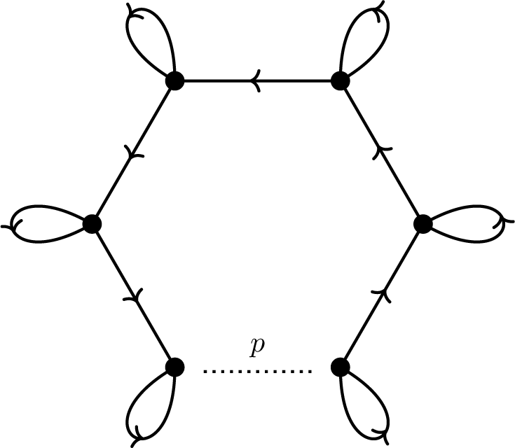
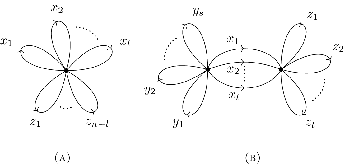


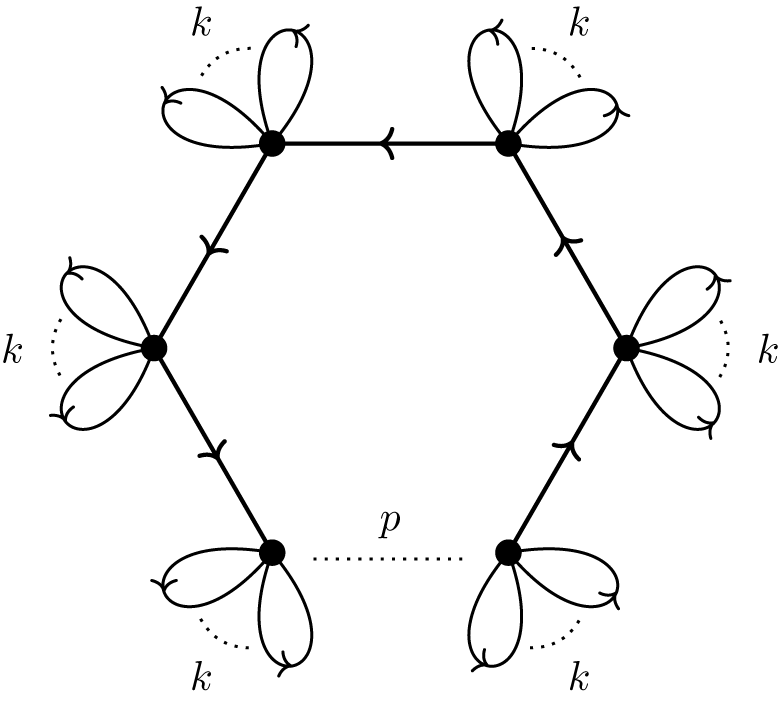


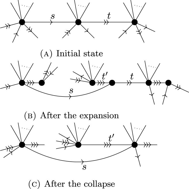
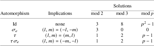
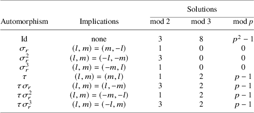
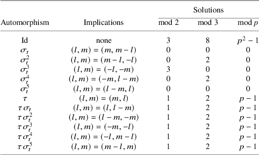
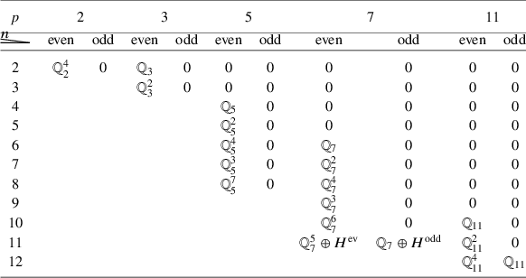

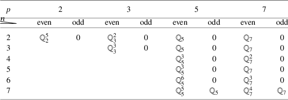


 Open access

