1. Introduction
Large-eddy simulation (LES) is an important approach for simulating turbulent flows. In LES, the large (or resolvable) scales of the flow field are explicitly computed while the effects of the smaller (subgrid) scales are modelled. The premise of LES is that if the energy-containing scales are well-resolved, then their statistics will be insensitive to the subgrid-scale (SGS) model, given that it extracts energy from the resolvable scales at the correct rate (Lilly Reference Lilly and Goldstine1967; Nieuwstadt & de Valk Reference Nieuwstadt and de Valk1987; Domaradzki, Liu & Brachet Reference Domaradzki, Liu and Brachet1993; Mason Reference Mason1994; Borue & Orszag Reference Borue and Orszag1998; Wyngaard Reference Wyngaard2004). This level of resolution requires the smallest resolvable scales to be in the inertial range. In LES of high-Reynolds-number turbulent boundary layers, however, the smallest resolvable scales in the near-wall region are inevitably in the energy-containing range (Kaimal et al. Reference Kaimal, Wyngaard, Izumi and Coté1972; Mason Reference Mason1994; Peltier et al. Reference Peltier, Wyngaard, Khanna and Brasseur1996; Tong et al. Reference Tong, Wyngaard, Khanna and Brasseur1998; Tong, Wyngaard & Brasseur Reference Tong, Wyngaard and Brasseur1999), leading to inherent under-resolution of the LES field. As a result, significant portions of the turbulent stress and scalar flux are carried by the subgrid scales, resulting in strong dependence of the near-wall LES results on the SGS model (e.g. Mason & Thomson Reference Mason and Thomson1992; Tong et al. Reference Tong, Wyngaard and Brasseur1999). Consequently, deficiencies in the SGS model are likely to have an adverse impact on near-wall LES statistics. For convective atmospheric boundary layers (ABLs), errors in the surface layer can also propagate into the mixed layer and alter the flow structure there (e.g. Khanna & Brasseur Reference Khanna and Brasseur1998; Ludwig, Chow & Street Reference Ludwig, Chow and Street2009), likely due to the upward turbulent transport.
To better understand the effects of the SGS turbulence on resolvable-scale statistics and those of the SGS model on LES statistics, Chen et al. (Reference Chen, Zhang, Wang and Tong2003) and Chen & Tong (Reference Chen and Tong2006) developed a statistical approach based on the evolution equation of the one-time, one-point joint probability density function (JPDF) of the resolvable-scale velocity, which contains all one-point resolvable-scale velocity statistics. They showed that the necessary conditions for LES to correctly predict the resolvable-scale velocity JPDF are that the conditional means of the SGS stress and SGS stress production rate must be reproduced by the SGS model. Similarly, the effects of the SGS temperature flux on the resolvable-scale potential temperature can be studied statistically using the transport equation of the one-time, one-point probability density function (PDF) of the resolvable-scale temperature, which shows that the necessary conditions for LES to correctly predict the resolvable-scale temperature PDF are that the conditional means of the SGS temperature flux and SGS temperature variance production rate must be reproduced by the SGS model.
Previous studies have successfully applied the JPDF equation to study the SGS dynamics, to identify SGS model deficiencies, and to evaluate SGS model performance in numerical simulations. A priori tests of the Smagorinsky model, the nonlinear model, the mixed model and the Kosović nonlinear model have found that, although these models can predict well certain components of the conditional mean SGS stress and SGS production rate, none are able to correctly predict both terms (Chen & Tong Reference Chen and Tong2006). The Smagorinsky model and the Kosović nonlinear model under-predict the anisotropy and the variations of the level of anisotropy, which are considered to be important for predicting the mean shear and the streamwise velocity variance, whereas the nonlinear model and the mixed model over-predict both. These results are consistent with a posteriori tests performed using the JPDF equation (Chen et al. Reference Chen, Otte, Sullivan and Tong2009).
To develop improved SGS parameterizations, additional physics, including history and non-local effects, must be incorporated into the SGS model. Transport-equation-based SGS models are well-suited for this purpose and have the potential to predict LES statistics with more accuracy (Deardorff Reference Deardorff1972, Reference Deardorff1973; Wyngaard Reference Wyngaard2004; Hatlee & Wyngaard Reference Hatlee and Wyngaard2007; Nguyen et al. Reference Nguyen, Horst, Oncley and Tong2013). Recent a posteriori tests of the transport-equation-based SGS model have found that the modelled SGS conservation equations could predict the conditional mean deviatoric SGS stress and its production rate better than could an eddy-diffusivity closure (Ramachandran Reference Ramachandran2010). Both, however, under-predict considerably the level of near-wall anisotropy. The enhanced performance of the transport-equation-based model was attributed to the inclusion of additional production and advection mechanisms that are absent in eddy-diffusivity closures, while its inability to predict correctly the SGS anisotropy was argued to be due to the absence of a model for the rapid pressure term in the modelled pressure–strain-rate correlation (Ramachandran & Wyngaard Reference Ramachandran and Wyngaard2011). Recent analyses of the full SGS transport equations by Nguyen et al. (Reference Nguyen, Horst, Oncley and Tong2013) using field measurement data, however, elucidated the role of the pressure–strain-rate correlation in the convective atmospheric surface layer and showed that it is the main cause of anisotropy, contrary to its commonly modelled role of causing return to isotropy. In the present study, we further investigate the SGS physics that govern the evolution of the resolvable-scale JPDF using the transport equations of the conditional mean SGS stress and SGS temperature flux.
In order for LES to predict correctly the resolvable-scale velocity JPDF and the resolvable-scale temperature PDF, the SGS model needs to predict the conditional mean SGS stress and the conditional mean SGS temperature flux. The former transports the velocity JPDF in both velocity and physical spaces, while the latter transports the temperature PDF in both scalar and physical spaces. To obtain the conditions for correctly predicting the conditional mean SGS stress and SGS flux, we utilize their transport equations, which are derived in appendix A following the method given by Pope (Reference Pope2010) for the self-conditioned LES field. The transport equation for the conditional mean SGS stress,
 $\langle {\it\tau}_{ij}|\boldsymbol{u}^{r}=\boldsymbol{v}\rangle$
, is
 $$\begin{eqnarray}\displaystyle \frac{\partial \left\langle {\it\tau}_{ij}|\boldsymbol{u}^{r}\right\rangle }{\partial t} & = & \displaystyle -v_{k}\frac{\partial \left\langle {\it\tau}_{ij}|\boldsymbol{u}^{r}\right\rangle }{\partial x_{k}}-\left\langle \left(\frac{\partial u_{l}^{r}}{\partial t}+u_{k}^{r}\frac{\partial u_{l}^{r}}{\partial x_{k}}\right)|\boldsymbol{u}^{r}\right\rangle \frac{\partial \left\langle {\it\tau}_{ij}|\boldsymbol{u}^{r}\right\rangle }{\partial v_{l}}\nonumber\\ \displaystyle & & \displaystyle +\,\left\langle \frac{\partial }{\partial x_{k}}\unicode[STIX]{x1D61B}_{ijk}^{(t)}|\boldsymbol{u}^{r}\right\rangle +\left\langle \unicode[STIX]{x1D617}_{ij}|\boldsymbol{u}^{r}\right\rangle +\left\langle \unicode[STIX]{x1D617}_{Bij}|\boldsymbol{u}^{r}\right\rangle +\left\langle {\it\Pi}_{ij}|\boldsymbol{u}^{r}\right\rangle -\left\langle {\it\epsilon}_{ij}|\boldsymbol{u}^{r}\right\rangle \nonumber\\ \displaystyle & & \displaystyle -\,\frac{1}{f_{u}}\frac{\partial }{\partial v_{l}}\left[\text{cov}\left({\it\tau}_{ij},\frac{\partial u_{l}^{r}}{\partial t}+u_{k}^{r}\frac{\partial u_{l}^{r}}{\partial x_{k}}|\boldsymbol{u}^{r}\right)f_{u}\right],\end{eqnarray}$$
where
 $\boldsymbol{u}$
is the velocity and
 ${\it\tau}_{ij}=(u_{i}u_{j})^{r}-u_{i}^{r}u_{j}^{r}$
is the conventional definition of the SGS stress (strictly, it is the SGS kinematic momentum flux or the negative of the apparent kinematic SGS stress), with superscript
 $r$
denoting a resolvable-scale variable. We refer to
 $\langle {\it\tau}_{ij}|\boldsymbol{u}^{r}=\boldsymbol{v}\rangle$
as the conditional mean SGS stress, defined to be the mean SGS stress obtained for given values of the resolvable-scale velocity. For convenience, the notation
 $\langle \cdot |\boldsymbol{u}^{r}=\boldsymbol{v}\rangle$
has been abbreviated to omit the velocity sample-space variable
 $\boldsymbol{v}$
in (1.1) and hereinafter. The first two terms on the right-hand side of (1.1) represent advection of the conditional mean SGS stress in physical and velocity spaces, respectively, with the latter due to the conditional mean resolvable-scale acceleration. The remaining terms are, in order, the conditional means of the turbulent transport of
 ${\it\tau}_{ij}$
 $$\begin{eqnarray}\frac{\partial }{\partial x_{k}}\unicode[STIX]{x1D61B}_{ijk}^{(t)}=\frac{\partial }{\partial x_{k}}\left[u_{k}^{r}\left(u_{i}u_{j}\right)^{r}-\left(u_{i}u_{j}u_{k}\right)^{r}+\left({\it\tau}_{ik}u_{j}^{r}+{\it\tau}_{jk}u_{i}^{r}\right)\right],\end{eqnarray}$$
the rate of mechanical production
 $$\begin{eqnarray}\unicode[STIX]{x1D617}_{ij}=-\left({\it\tau}_{ik}\frac{\partial u_{j}^{r}}{\partial x_{k}}+{\it\tau}_{jk}\frac{\partial u_{i}^{r}}{\partial x_{k}}\right),\end{eqnarray}$$
the rate of buoyant production
 $$\begin{eqnarray}\unicode[STIX]{x1D617}_{Bij}=\frac{g}{{\it\Theta}}\left\{{\it\delta}_{i3}\left[({\it\theta}u_{j})^{r}-{\it\theta}^{r}u_{j}^{r}\right]+{\it\delta}_{j3}\left[({\it\theta}u_{i})^{r}-{\it\theta}^{r}u_{i}^{r}\right]\right\}\!,\end{eqnarray}$$
the velocity–pressure-gradient correlation
 $$\begin{eqnarray}{\it\Pi}_{ij}=-\left[\left(u_{i}\frac{\partial p}{\partial x_{j}}+u_{j}\frac{\partial p}{\partial x_{i}}\right)^{r}-\left(u_{i}^{r}\frac{\partial p^{r}}{\partial x_{j}}+u_{j}^{r}\frac{\partial p^{r}}{\partial x_{i}}\right)\right],\end{eqnarray}$$
and the rate of viscous dissipation and transport,
 $$\begin{eqnarray}{\it\epsilon}_{ij}=2{\it\nu}\left[\left(\frac{\partial u_{i}}{\partial x_{k}}\frac{\partial u_{j}}{\partial x_{k}}\right)^{r}-\frac{\partial u_{i}^{r}}{\partial x_{k}}\frac{\partial u_{j}^{r}}{\partial x_{k}}\right]+{\it\nu}\frac{\partial ^{2}{\it\tau}_{ij}}{\partial x_{k}\partial x_{k}},\end{eqnarray}$$
where
 ${\it\Theta}$
,
 ${\it\theta}$
,
 $p$
,
 $g$
and
 ${\it\nu}$
are the mean and fluctuating potential temperatures, kinematic pressure, gravitational acceleration and kinematic viscosity, respectively, and
 ${\it\delta}_{ij}$
is the Kronecker delta. For high-Reynolds-number flows, viscous transport is small and viscous dissipation is almost entirely in the subgrid scales since the smallest resolvable scales are much larger than the Kolmogorov scale in the surface layer. The last term in (1.1) is the covariance of the conditional mean fluctuations of the SGS stress and the conditional mean resolvable-scale acceleration. The SGS velocity–pressure-gradient correlation can be decomposed into a pressure–strain-rate correlation and a pressure transport term,
 $$\begin{eqnarray}{\it\Pi}_{ij}=\mathscr{R}_{ij}-\frac{\partial }{\partial x_{k}}\unicode[STIX]{x1D61B}_{ijk}^{(p)},\end{eqnarray}$$
respectively, where
 $$\begin{eqnarray}\mathscr{R}_{ij}=\left(p\frac{\partial u_{i}}{\partial x_{j}}+p\frac{\partial u_{j}}{\partial x_{i}}\right)^{r}-\left(p^{r}\frac{\partial u_{i}^{r}}{\partial x_{j}}+p^{r}\frac{\partial u_{j}^{r}}{\partial x_{i}}\right)\end{eqnarray}$$
is the SGS pressure–strain-rate correlation tensor, and
 $$\begin{eqnarray}\unicode[STIX]{x1D61B}_{ijk}^{(p)}={\it\delta}_{jk}\left[(pu_{i})^{r}-p^{r}u_{i}^{r}\right]+{\it\delta}_{ik}\left[(pu_{j})^{r}-p^{r}u_{j}^{r}\right]\!.\end{eqnarray}$$
The trace of
 $\mathscr{R}_{ij}$
is zero, consequently the pressure–strain-rate correlation acts to redistribute energy among the three normal SGS stress components.
Equation (1.1) provides the necessary conditions for LES to correctly predict the conditional mean SGS stress: the conditional mean SGS mechanical and buoyant production, the conditional mean SGS turbulent and pressure transport, the conditional mean SGS pressure–strain-rate correlation, and the conditional mean SGS dissipation must be reproduced by the SGS model. Since it is necessary to correctly predict the conditional mean SGS production in order to correctly model the conditional mean SGS stress, the necessary conditions for correctly predicting the resolvable-scale velocity JPDF are also implicitly satisfied. Similar to Reynolds stress modelling, the main challenge in transport-equation-based LES is expected to come from modelling of the pressure–strain-rate correlation.
The transport equation for the conditional mean SGS temperature flux,
 $\langle F_{i}|{\it\theta}^{r}={\it\psi}\rangle$
, also derived in appendix A, is
 $$\begin{eqnarray}\displaystyle \frac{\partial \!\left\langle F_{i}|{\it\theta}^{r}\right\rangle }{\partial t} & = & \displaystyle -\left\{\left\langle u_{k}^{r}|{\it\theta}^{r}\right\rangle \frac{\partial \!\left\langle F_{i}|{\it\theta}^{r}\right\rangle }{\partial x_{k}}+\text{cov}\left(u_{k}^{r},\frac{\partial F_{i}}{\partial x_{k}}|{\it\theta}^{r}\right)\right\}\nonumber\\ \displaystyle & & \displaystyle -\,\left\langle \left(\frac{\partial {\it\theta}^{r}}{\partial t}+\left\langle u_{k}^{r}|{\it\theta}^{r}\right\rangle \frac{\partial {\it\theta}^{r}}{\partial x_{k}}\right)|{\it\theta}^{r}\right\rangle \frac{\partial \left\langle F_{i}|{\it\theta}^{r}\right\rangle }{\partial {\it\psi}}\nonumber\\ \displaystyle & & \displaystyle +\,\left\langle \frac{\partial }{\partial x_{k}}\unicode[STIX]{x1D61B}_{Fik}^{(t)}|{\it\theta}^{r}\right\rangle +\left\langle P_{\mathit{Fi}}|{\it\theta}^{r}\right\rangle +\left\langle P_{BFi}|{\it\theta}^{r}\right\rangle +\left\langle {\it\Pi}_{\mathit{Fi}}|{\it\theta}^{r}\right\rangle \nonumber\\ \displaystyle & & \displaystyle -\,\frac{1}{f_{{\it\theta}}}\frac{\partial }{\partial {\it\psi}}\left[\text{cov}\left(F_{i},\frac{\partial {\it\theta}^{r}}{\partial t}+\left\langle u_{k}^{r}|{\it\theta}^{r}\right\rangle \frac{\partial {\it\theta}^{r}}{\partial x_{k}}|{\it\theta}^{r}\right)f_{{\it\theta}}\right],\end{eqnarray}$$
where
 $F_{i}=({\it\theta}u_{i})^{r}-{\it\theta}^{r}u_{i}^{r}$
is the SGS temperature flux in the
 $i$
-direction. We refer to
 $\langle F_{i}|{\it\theta}^{r}={\it\psi}\rangle$
as the conditional mean SGS temperature flux, defined to be the mean SGS temperature flux obtained for given values of the resolvable-scale temperature. Similarly, the notation
 $\langle \cdot |{\it\theta}^{r}={\it\psi}\rangle$
has been abbreviated to omit the potential temperature sample-space variable
 ${\it\psi}$
in (1.10) and hereinafter. The first two terms on the right-hand side of (1.10) represent advection of the conditional mean SGS temperature flux in physical and scalar spaces, respectively, with the latter due to the total time rate of change of the conditioning variable (the resolvable-scale temperature). The remaining terms are, in order, the conditional means of the turbulent transport of
 $F_{i}$
 $$\begin{eqnarray}\frac{\partial }{\partial x_{k}}\unicode[STIX]{x1D61B}_{Fik}^{(t)}=-\frac{\partial }{\partial x_{k}}\left[\left({\it\theta}u_{i}u_{k}\right)^{r}-{\it\theta}^{r}\left(u_{i}u_{k}\right)^{r}-u_{i}^{r}\left({\it\theta}u_{k}\right)^{r}-u_{k}^{r}\left({\it\theta}u_{i}\right)^{r}+2{\it\theta}^{r}u_{i}^{r}u_{k}^{r}\right]\!,\end{eqnarray}$$
the rate of gradient (stratification) production and tilting production
 $$\begin{eqnarray}P_{\mathit{Fi}}=-{\it\tau}_{ik}\frac{\partial {\it\theta}^{r}}{\partial x_{k}}-F_{k}\frac{\partial u_{i}^{r}}{\partial x_{k}},\end{eqnarray}$$
respectively, the rate of buoyant production
 $$\begin{eqnarray}P_{BFi}={\it\delta}_{i3}\frac{g}{{\it\Theta}}\left[({\it\theta}^{2})^{r}-\left({\it\theta}^{r}\right)^{2}\right]\!,\end{eqnarray}$$
and the temperature–pressure-gradient correlation
 $$\begin{eqnarray}{\it\Pi}_{\mathit{Fi}}=-\left[\left({\it\theta}\frac{\partial p}{\partial x_{i}}\right)^{r}-{\it\theta}^{r}\frac{\partial p^{r}}{\partial x_{i}}\right].\end{eqnarray}$$
The last term in (1.10) is the covariance of the conditional mean fluctuations of the SGS flux and the substantial derivative of the resolvable-scale temperature. Note that the SGS temperature–pressure-gradient correlation can be decomposed into a correlation between the fluctuating pressure and temperature gradient, and a transport term representing heat flux divergences due to the fluctuating pressure,
 $$\begin{eqnarray}{\it\Pi}_{\mathit{Fi}}=\mathscr{R}_{\mathit{Fi}}-\frac{\partial }{\partial x_{k}}\unicode[STIX]{x1D61B}_{Fik}^{(p)},\end{eqnarray}$$
respectively, where
 $$\begin{eqnarray}\mathscr{R}_{\mathit{Fi}}=\left(p\frac{\partial {\it\theta}}{\partial x_{i}}\right)^{r}-p^{r}\frac{\partial {\it\theta}^{r}}{\partial x_{i}}\end{eqnarray}$$
and
 $$\begin{eqnarray}\unicode[STIX]{x1D61B}_{Fik}^{(p)}={\it\delta}_{ik}\left[\left(p{\it\theta}\right)^{r}-p^{r}{\it\theta}^{r}\right].\end{eqnarray}$$
Equation (1.10) provides the necessary conditions for LES to correctly predict the conditional mean SGS temperature flux: the conditional mean SGS gradient, tilting and buoyant production, the conditional mean SGS turbulent and pressure transport, and the conditional mean SGS pressure–temperature-gradient correlation must be reproduced by the SGS model. Although the production terms for both the SGS stress and SGS flux are not directly modelled, they must be correctly predicted by the SGS model. Based on these conditions, investigations of the physics of the SGS stress and scalar flux should therefore focus on the conditional mean budget terms. In the present study, we analyse these budget terms and their dependence on the stability condition and filter width using field measurement data.
The rest of the paper is organized as follows. Section 2 outlines the field campaign and the use of sensor arrays to obtain resolvable- and subgrid-scale variables. Section 3 examines the dependence of the measured SGS terms on the surface layer stability and the filter width: the results for the conditional mean SGS stress and the conditional mean SGS temperature flux are presented in § 3.1, term-by-term analyses of their budgets are presented in §§ 3.2 and 3.3, and the combined effects of the budgets terms on the conditional mean SGS stress are summarized in § 3.4. Discussion and conclusions are given in § 4. Derivations of the transport equations are presented in appendix A.
2. AHATS field campaign
The field measurements for this study, named the Advection Horizontal Array Turbulence Study (AHATS), were conducted in the San Joaquin Valley, California, during the summer of 2008 as a collaboration between Clemson University, Penn State University, and the National Center for Atmospheric Research (NCAR). Horst et al. (Reference Horst, Kleissl, Lenschow, Meneveau, Moeng, Parlange, Sullivan and Weil2004) and Nguyen et al. (Reference Nguyen, Horst, Oncley and Tong2013) describe the field site in detail. The field measurement design is based on the transverse array technique, proposed, studied and first implemented successfully by Tong et al. (Reference Tong, Wyngaard, Khanna and Brasseur1997, Reference Tong, Wyngaard, Khanna and Brasseur1998, Reference Tong, Wyngaard and Brasseur1999) for surface-layer measurements in the ABL. In the context of LES, the technique uses horizontal sensor arrays to perform two-dimensional filtering to obtain resolvable- and subgrid-scale variables. It has subsequently been implemented by others in the ABL over land and ocean (Porté-Agel et al. Reference Porté-Agel, Parlange, Meneveau and Eichinger2001; Kleissl, Meneveau & Parlange Reference Kleissl, Meneveau and Parlange2003; Horst et al. Reference Horst, Kleissl, Lenschow, Meneveau, Moeng, Parlange, Sullivan and Weil2004; Sullivan et al. Reference Sullivan, Edson, Horst, Wyngaard and Kelly2006), within vegetation (Patton et al. Reference Patton, Horst, Sullivan, Lenschow, Oncley, Brown, Burns, Guenther, Held, Karl, Mayor, Rizzo, Spuler, Sun, Turnipseed, Allwine, Edburg, Lamb, Avissar, Calhoun, Kleissl, Massman, Paw-U and Weil2011), over a glacier (Bou-Zeid et al. Reference Bou-Zeid, Higgins, Huwald, Meneveau and Parlange2010), and in engineering flows (Cerutti, Meneveau & Knio Reference Cerutti, Meneveau and Knio2000; Tong Reference Tong2001; Wang & Tong Reference Wang and Tong2002; Chen et al. Reference Chen, Zhang, Wang and Tong2003; Rajagopalan & Tong Reference Rajagopalan and Tong2003; Wang, Tong & Pope Reference Wang, Tong and Pope2004). Similar to these field studies, AHATS uses two vertically spaced arrays of sensors, shown in figure 1(b), to obtain filtered variables and their derivatives. The arrays are centred in the lateral direction and aligned perpendicular to the prevailing wind direction.
(a) Top view of arrays. The upwind and downwind arrays are centred laterally, with
 $d_{x}$
denoting their streamwise separation distance. Due to variations in the run-averaged wind direction, we rotate the coordinate system and interpolate the velocity, temperature and pressure in the virtual Cartesian coordinate system defined by the mean alongwind and crosswind directions. (b) Front view of downwind array. Sonic anemometers

 $z_{p}$
and
 $z_{s}$
, respectively; the horizontal spacing is
 $d_{y}$
. Pressure ports


In AHATS, a third line of sonic anemometers was added upwind to measure spatial differences in the streamwise direction (figure 1
a). Additionally, two lines of turbulent pressure probes were added to measure, for the first time, the resolvable- and subgrid-scale pressure. The pressure probes are modified commercial versions of the quad-disk design by Nishiyama & Bedard (Reference Nishiyama and Bedard1991), which are insensitive to velocity fluctuations and are capable of measuring pressure covariances with reasonable accuracy (Wyngaard, Siegel & Wilczak Reference Wyngaard, Siegel and Wilczak1994). The pressure probes are mounted level with the sonic anemometers and are offset slightly in the along- and cross-wind directions (figure 1
c) relative to the sonic anemometers to avoid flow-induced distortion of the velocity measurements (Wyngaard Reference Wyngaard1981; Miller, Tong & Wyngaard Reference Miller, Tong and Wyngaard1999). Each probe is connected to a differential pressure transducer (Paroscientific Model 202BG), the reference side of which is connected to a common reference reservoir. Following Wilczak & Bedard (Reference Wilczak and Bedard2004), the reference reservoir is filled with loosely packed steel wool and buried to prevent generation of dynamic pressure from convection and to maintain a uniform temperature (and hence pressure) through conduction. However, due to persistent low-frequency pressure fluctuations within the reference system induced by radiative heating and advective cooling of the reference tubing, an additional transducer was added to measure the reference pressure using a second reference reservoir. The absolute pressure is obtained by adding the reference pressure back to the measured (probe) pressure. This pressure signal still contains some residual low-frequency fluctuations (
 ${<}$
0.05 Hz). However, because the lengths of the reference tubes are on the order of 10 m, the pipe-organ resonance frequencies are much higher; therefore, the tubes do not support acoustic waves of such low frequencies. Helmholtz resonance, if it exists, would be very weak and at much higher frequencies since the reference system is sealed. Thus, the low-frequency fluctuations have the same phase and affect the signals of all the pressure transducers in the same way. The fluctuations were found to affect the pressure terms in the Reynolds stress budget as well as those in the SGS stress budget for very large filter widths (those much larger than the horizontal integral length scale of the vertical velocity). Thus, we only obtain the SGS pressure terms for filter widths smaller than those of the energy-containing eddies.
In the present study, we use the arrays to approximate top-hat filters. In the streamwise direction, adoption of Taylor’s hypothesis (Lumley Reference Lumley1965) allows using the time-filtered signal as a surrogate for streamwise spatial filtering. Filtering in the transverse direction is performed by weight-averaging the output of the sensor array (Tong et al. Reference Tong, Wyngaard, Khanna and Brasseur1998). Streamwise and spanwise derivatives are approximated using fourth-order central finite-difference schemes, while vertical derivatives are approximated using a first-order one-sided finite difference scheme. The validity of the array filtering technique, including the accuracy of two-dimensional filtering and use of Taylor’s hypothesis, has been thoroughly studied. Using a spectral cutoff array filter, Tong et al. (Reference Tong, Wyngaard, Khanna and Brasseur1998) showed that the r.m.s. values of the filtered variables differed from that of a true spectral cutoff filter by less than 10 %. The accuracy of the top-hat array filter is expected to be higher (Chen & Tong Reference Chen and Tong2006). They also showed two-dimensional filtering to be a good approximation of three-dimensional filtering with a 10 %–14 % higher variance. Field measurements by Higgins, Parlange & Meneveau (Reference Higgins, Parlange and Meneveau2007) confirmed this result and showed that the difference can be interpreted as a 16 % reduction in the filter size. Tong et al. (Reference Tong, Wyngaard, Khanna and Brasseur1998) showed that among the mechanisms that could affect the accuracy of Taylor’s hypothesis, including the effects of different convecting velocities for different wavenumber components, temporal changes in the reference moving with the mean velocity, and the fluctuating convecting velocity, only the last was significant. Kleissl et al. (Reference Kleissl, Meneveau and Parlange2003) studied the errors associated with approximating gradients by finite differences; they evaluated the divergence-free condition for the filtered velocity field using fourth- and first-order finite difference schemes for the horizontal and vertical derivatives, respectively, and concluded that the errors were acceptable for studying the SGS dynamics. Horst et al. (Reference Horst, Kleissl, Lenschow, Meneveau, Moeng, Parlange, Sullivan and Weil2004) further examined various issues of using the array technique, including the aliasing errors associated with evaluating derivatives using finite differences, and furthermore demonstrated reasonable accuracy of the technique.
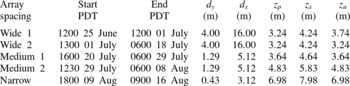
Five different array configurations, shown in table 1, are employed in AHATS in order to vary the filter (grid) aspect ratio,
 $z/{\it\Delta}_{f}$
, and the stability parameter,
 $z/L$
, where
 $z$
,
 ${\it\Delta}_{f}$
and
 $L=-(u_{\ast }^{3}{\it\Theta})/({\it\kappa}g\langle u_{3}^{\prime }{\it\theta}^{\prime }\rangle )$
are the height above the ground, the filter width, and the Monin–Obukhov length, respectively, with primes denoting fluctuations and angle brackets denoting an ensemble average. We refer to
 $z$
as the height of the primary array
 $z_{p}$
here and hereinafter. Note,
 ${\it\kappa}=0.41$
,
 $u_{\ast }=(-\langle u_{1}^{\prime }u_{3}^{\prime }\rangle )^{1/2}$
(with
 $u_{1}^{\prime }$
in the mean wind direction) and
 $\langle u_{3}^{\prime }{\it\theta}^{\prime }\rangle =Q_{0}$
are the von Kármán constant, the friction velocity and the vertical temperature flux, respectively. We define the surface-layer temperature scale by
 $T_{\ast }=-Q_{0}/u_{\ast }$
. In the present work, we study the unstable surface layer (i.e. for which
 $z/L<0$
) using data from the medium and wide array configurations. The resolved fields are obtained using several different filter widths, resulting in a filter aspect ratio ranging from 0.10 to 1.87 and therefore allowing for the effects of grid anisotropy to be studied. We use 26 data segments, each generally 30–90 min in length, collected during the daytime and spanning a wide range of
 $-z/L$
. Each data segment has a steady mean velocity and approximately stationary fluctuating velocities. The lengths for most datasets correspond to approximately 2000 advection time scales of the vertical-velocity energy-containing eddies (evaluated as the ratio of the length of each dataset to its advection time scale,
 $t_{a}=z/U$
, where
 $U$
is the mean velocity in the alongwind direction); and, although the precise level of statistical uncertainty is difficult to determine for the statistics obtained, it is sufficiently low for determining the dependence of the statistics on the important parameters discussed in § 3.
AHATS array configurations, with
 $z_{u}$
denoting the height of the upwind array. The streamwise array separation distance,
 $d_{x}$
, was chosen to minimize flow distortion at the downwind array.

3. Results
In the following, we study the evolution of the conditional mean SGS stress and the conditional mean SGS temperature flux by analysing term-by-term their transport equations. A summary of the combined effects of the budget terms on the conditional mean SGS stress is given in § 3.4. The dependence of the budget terms on the surface-layer stability and filter width are examined using two non-dimensional parameters,
 $z/L$
and
 ${\it\Lambda}_{w}/{\it\Delta}_{f}$
, where
 ${\it\Lambda}_{w}$
is the wavelength corresponding to the peak of the vertical-velocity spectrum (i.e. the horizontal integral length scale of the vertical velocity). The dimensionless height,
 $z/L$
, is a measure of the stability of the surface layer. The wavelength–filter-width ratio,
 ${\it\Lambda}_{w}/{\it\Delta}_{f}$
, is a measure of the resolution of the filter relative to the turbulence field (i.e. a large value of
 ${\it\Lambda}_{w}/{\it\Delta}_{f}$
corresponds to a filter width much smaller than the energy-containing scales, and therefore a well-resolved LES field). Following Sullivan et al. (Reference Sullivan, Horst, Lenschow, Moeng and Weil2003), we assume
 ${\it\Lambda}_{w}=2{\rm\pi}Ut_{f}$
using Taylor’s hypothesis, and determine the Eulerian integral time scale
 $t_{f}$
by fitting an exponential of the form
 ${\it\rho}(t)=\exp (-t/t_{f})$
to the autocorrelation function of the vertical velocity (Lenschow, Mann & Kristensen Reference Lenschow, Mann and Kristensen1993; Kaimal & Finnigan Reference Kaimal and Finnigan1994). For sufficiently convective surface layers (
 $-z/L>0.2$
), the ratio
 $z/{\it\Lambda}_{w}$
is constant.
In the present study, the SGS statistics are non-dimensionalized using surface-layer scaling: the conditional mean SGS pressure and conditional mean SGS stress are normalized by
 $u_{\ast }^{2}$
, while the budget terms in the transport equation of the conditional mean SGS stress are normalized by
 ${\it\kappa}z/u_{\ast }^{3}$
. The conditional mean temperature flux is normalized by
 $T_{\ast }u_{\ast }$
, while the budget terms in its transport equation are normalized by
 ${\it\kappa}z/(T_{\ast }u_{\ast }^{2})$
.
The measured SGS stress and its budget terms are conditioned on the fluctuating parts of the streamwise and vertical components of the resolvable-scale velocity (
 $u_{1}^{r}$
and
 $u_{3}^{r}$
, respectively), both of which are normalized by their respective resolved-scale r.m.s. values. The spanwise velocity component,
 $u_{2}^{r}$
, plays a lesser role in the dynamics of the SGS stress (Chen & Tong Reference Chen and Tong2006; Chen et al.
Reference Chen, Otte, Sullivan and Tong2009), and therefore is not included as a conditioning variable for most terms. The measured SGS temperature flux and its budget terms are conditioned on the fluctuating part of the resolvable-scale potential temperature,
 ${\it\theta}^{r}$
, normalized by its resolved-scale r.m.s. value. Conditional mean statistics are obtained using the first-order kernel density estimation method (Wand & Jones Reference Wand and Jones1995), resulting in faster convergence and lower bias. We limit the results to the central part of the sample space containing at least 99.5 % of the probability of the velocity and temperature PDFs. To achieve further statistical convergence, we weight-average and combine the results for data sets collected under similar stability conditions with comparable values of
 ${\it\Lambda}_{w}/{\it\Delta}_{f}$
.
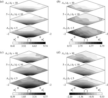
Conditional mean of the measured SGS stress components for the strongly convective (
 $0.8<-z/L\leqslant 1.5$
, with mean
 $-z/L=1.14$
) surface layer. (a)
 $\langle {\it\tau}_{11}|u_{1}^{r},u_{3}^{r}\rangle$
;(b)
 $\langle {\it\tau}_{22}|u_{2}^{r},u_{3}^{r}\rangle$
; (c)
 $\langle {\it\tau}_{33}|u_{1}^{r},u_{3}^{r}\rangle$
; (d)
 $\langle {\it\tau}_{13}|u_{1}^{r},u_{3}^{r}\rangle$
.

3.1. Conditional mean SGS stress and SGS temperature flux
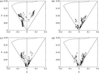
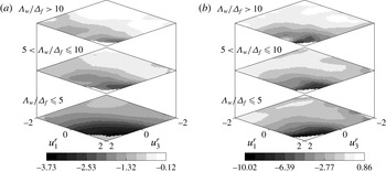
Following previous studies of SGS physics in the weakly convective atmospheric surface layer (Chen & Tong Reference Chen and Tong2006; Chen, Liu & Tong Reference Chen, Liu and Tong2010), we first present the results for the conditional mean SGS stress and SGS temperature flux and examine their filter-scale dependence in the strongly convective surface layer. The results for the conditional mean SGS stress (figure 2) show that
 $\langle {\it\tau}_{ij}|\boldsymbol{u}^{r}\rangle$
generally increases with
 $u_{1}^{r}$
(
 $u_{2}^{r}$
) and
 $u_{3}^{r}$
due to the stronger vertical shear and buoyancy acceleration. To better understand the effects of the filter width, we characterize the level of anisotropy of
 $\langle {\it\tau}_{ij}|\boldsymbol{u}^{r}\rangle$
in figure 3 using the Lumley triangle (Lumley Reference Lumley1978). Here, the two invariants,
 ${\it\xi}$
and
 ${\it\eta}$
, of the normalized anisotropy tensor
 $$\begin{eqnarray}\langle \unicode[STIX]{x1D623}_{ij}|\boldsymbol{u}^{r}\rangle =\frac{\langle {\it\tau}_{ij}|\boldsymbol{u}^{r}\rangle }{\langle {\it\tau}_{kk}|\boldsymbol{u}^{r}\rangle }-\frac{1}{3}{\it\delta}_{ij}\end{eqnarray}$$
defined by Pope (Reference Pope2000),
 $$\begin{eqnarray}\displaystyle & 6{\it\xi}^{3}\equiv 3\text{III}_{b}=\langle \unicode[STIX]{x1D623}_{ii}|\boldsymbol{u}^{r}\rangle ^{3}=\langle \unicode[STIX]{x1D623}_{ij}|\boldsymbol{u}^{r}\rangle \langle \unicode[STIX]{x1D623}_{jk}|\boldsymbol{u}^{r}\rangle \langle \unicode[STIX]{x1D623}_{ki}|\boldsymbol{u}^{r}\rangle , & \displaystyle\end{eqnarray}$$
 $$\begin{eqnarray}\displaystyle & 6{\it\eta}^{2}\equiv -2\text{II}_{b}=\langle \unicode[STIX]{x1D623}_{ii}|\boldsymbol{u}^{r}\rangle ^{2}=\langle \unicode[STIX]{x1D623}_{ij}|\boldsymbol{u}^{r}\rangle \langle \unicode[STIX]{x1D623}_{ji}|\boldsymbol{u}^{r}\rangle , & \displaystyle\end{eqnarray}$$
 $\langle {\it\tau}_{ij}|\boldsymbol{u}^{r}\rangle$
is isotropic, both
 ${\it\xi}$
and
 ${\it\eta}$
are zero. The results in figure 3 show that the conditional mean SGS stress is generally close to axisymmetric and is less anisotropic (smaller values of
 ${\it\xi}$
and
 ${\it\eta}$
) for the strongly convective surface layer than for the weakly convective one due to the weaker vertical shear. For large filter widths, figure 3(a,c) shows that
 $\langle {\it\tau}_{ij}|\boldsymbol{u}^{r}\rangle$
is quite anisotropic when
 $u_{3}^{r}$
is positive. For negative
 $u_{1}^{r}$
, the state of anisotropy is close to
 ${\it\eta}=-{\it\xi}$
(one small eigenvalue) since the SGS stress is more horizontally isotropic due to the weaker vertical shear. For positive
 $u_{1}^{r}$
, it transitions toward
 ${\it\eta}={\it\xi}$
(one large eigenvalue) due to stronger shear. When
 $u_{3}^{r}$
is negative, the SGS stress is generally much less anisotropic.
The Lumley triangle representation of the invariants,
 ${\it\xi}$
and
 ${\it\eta}$
, characterizing the anisotropy of the conditional mean SGS stress for the (a,b) weakly convective (
 $0<-z/L\leqslant 0.8$
) and (c,d) strongly convective (
 $0.8<-z/L\leqslant 1.5$
) surface layers. Arrows represent the conditioning velocity vector (
 $u_{1}^{r},u_{3}^{r}$
). (a,c)
 ${\it\Lambda}_{w}/{\it\Delta}_{f}\leqslant 5$
; (b,d)
 ${\it\Lambda}_{w}/{\it\Delta}_{f}>10$
.

As the filter width decreases (figure 3
b,d), the state of anisotropy tends to move toward
 ${\it\eta}={\it\xi}$
, indicating that
 $\langle {\it\tau}_{ij}|\boldsymbol{u}^{r}\rangle$
is close to axisymmetric with one large eigenvalue. This change is consistent with the fact that the peaks of the
 $u$
and
 $v$
spectra occur at lower wavenumbers than that of the
 $w$
spectrum (Kaimal et al.
Reference Kaimal, Wyngaard, Izumi and Coté1972), and therefore a smaller filter width will cause
 $\langle {\it\tau}_{11}|\boldsymbol{u}^{r}\rangle$
and
 $\langle {\it\tau}_{22}|\boldsymbol{u}^{r}\rangle$
to fall off much faster than
 $\langle {\it\tau}_{33}|\boldsymbol{u}^{r}\rangle$
. In addition, the shear production plays a greater role, resulting in larger magnitudes of
 $\langle {\it\tau}_{11}|\boldsymbol{u}^{r}\rangle$
compared to
 $\langle {\it\tau}_{22}|\boldsymbol{u}^{r}\rangle$
(figure 2). For very small filter widths, however, the SGS stress appears to approach isotropy. The results also show that the peak of the conditional mean SGS stress decreases by at most 40 % when the filter width is decreased by a factor of 5 (figure 2), while the magnitude of the (unconditional) mean SGS stress
 $\langle {\it\tau}_{ij}\rangle$
decreases by nearly 60 % for the same filter width reduction (Nguyen et al.
Reference Nguyen, Horst, Oncley and Tong2013). Therefore, although it is less anisotropic, the dependence of
 $\langle {\it\tau}_{ij}|\boldsymbol{u}^{r}\rangle /\langle {\it\tau}_{ij}\rangle$
(the magnitude of the conditional mean SGS stress relative to its unconditional mean) on
 $\boldsymbol{u}^{r}$
does not become weaker as the filter width decreases, contrary to the notion of local isotropy, which suggests that the dependence of SGS stress on the resolvable-scale velocity should weaken.
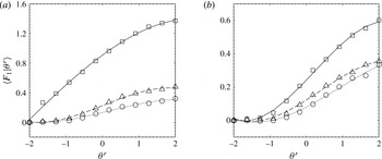
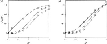
Conditional mean of the measured SGS horizontal temperature flux for the (a) weakly convective (
 $0<-z/L\leqslant 1$
, with mean
 $-z/L=0.45$
) and (b) strongly convective (
 $1<-z/L\leqslant 2.5$
, with mean
 $-z/L=1.70$
) surface layers and varying values of the wavelength–filter-width ratio: ▫,
 ${\it\Lambda}_{w}/{\it\Delta}_{f}\leqslant 5$
; ▵,
 $5<{\it\Lambda}_{w}/{\it\Delta}_{f}\leqslant 10$
;○,
 ${\it\Lambda}_{w}/{\it\Delta}_{f}>10$
.

Conditional mean of the measured SGS vertical temperature flux for the (a) weakly convective (
 $0<-z/L\leqslant 1$
, with mean
 $-z/L=0.45$
) and (b) strongly convective (
 $1<-z/L\leqslant 2.5$
, with mean
 $-z/L=1.70$
) surface layers. The data are grouped as in figure 4.

The horizontal and vertical components of the conditional mean SGS potential temperature flux,
 $\langle F_{1}|{\it\theta}^{r}\rangle$
and
 $\langle F_{3}|{\it\theta}^{r}\rangle$
, are shown in figures 4 and 5, respectively, for the weakly and strongly convective surface layers. We note that the non-dimensionalized conditional mean fluxes have opposite signs relative to the actual fluxes since
 $T_{\ast }<0$
for unstable surface layers. The results show that
 $\langle F_{1}|{\it\theta}^{r}\rangle$
(
 $\langle F_{3}|{\it\theta}^{r}\rangle$
) is positive (negative) and increases in magnitude with
 ${\it\theta}^{r}$
. For negative
 ${\it\theta}^{r}$
, the magnitude of
 $\langle F_{i}|{\it\theta}^{r}\rangle$
is smaller and its dependence on
 ${\it\theta}^{r}$
is weaker. It also decreases with increasing
 ${\it\Lambda}_{w}/{\it\Delta}_{f}$
since the SGS temperature flux is more isotropic for smaller filter widths. The horizontal flux is weaker for the strongly convective surface layer since, in a horizontally homogeneous surface layer, horizontal scalar flux is produced primarily by tilting of vertical scalar flux by vertical wind shear (Hatlee & Wyngaard Reference Hatlee and Wyngaard2007; Chen et al.
Reference Chen, Liu and Tong2010), which disappears under free convection. In contrast, the vertical flux appears to be much less dependent on the surface-layer instability. Similar to the conditional mean SGS stress, the conditional mean SGS temperature flux has a non-diminishing dependence on the resolvable-scale temperature for all filter widths, although its level of anisotropy decreases. Figures 4 and 5 show that the peaks of the conditional mean SGS horizontal and vertical fluxes decrease by at most 50 % when the filter width is decreased by a factor of 5, although the magnitudes of the mean fluxes decrease by nearly 70 % for the same filter width reduction (Nguyen et al.
Reference Nguyen, Horst, Oncley and Tong2013). Therefore, although it is less anisotropic, the dependence of the normalized conditional mean SGS temperature flux
 $\langle F_{i}|{\it\theta}^{r}\rangle /\langle F_{i}\rangle$
does not become weaker as the filter width decreases, suggesting that it has a strong influence on the resolvable-scale temperature PDF even for inertial-range filter widths.
3.2. Conditional mean SGS stress budget
3.2.1. Conditional mean SGS production
The results for the conditional mean SGS production rate show that the trends of
 $\langle \unicode[STIX]{x1D617}_{11}|\boldsymbol{u}^{r}\rangle$
and
 $\langle \unicode[STIX]{x1D617}_{22}|\boldsymbol{u}^{r}\rangle$
are similar to those of
 $\langle {\it\tau}_{11}|\boldsymbol{u}^{r}\rangle$
and
 $\langle {\it\tau}_{22}|\boldsymbol{u}^{r}\rangle$
(generally increasing with
 $u_{3}^{r}$
) and therefore are not repeated here. The trends of
 $\langle \unicode[STIX]{x1D617}_{B33}|\boldsymbol{u}^{r}\rangle$
are similar to those of
 $\langle {\it\tau}_{33}|\boldsymbol{u}^{r}\rangle$
, while
 $\langle \unicode[STIX]{x1D617}_{33}|\boldsymbol{u}^{r}\rangle$
generally decreases with
 $u_{3}^{r}$
. Instead, to better understand the conditional energy transfer among the normal components of the SGS stress by
 $\langle \unicode[STIX]{x1D617}_{{\it\alpha}{\it\alpha}}|\boldsymbol{u}^{r}\rangle$
, we examine the deviatoric and isotropic contributions of the production tensor,
 $\unicode[STIX]{x1D617}_{ij}=\unicode[STIX]{x1D617}_{ij}^{d}-(2/3){\it\tau}_{kk}\unicode[STIX]{x1D61A}_{ij}$
, where
 $\unicode[STIX]{x1D617}_{ij}^{d}=-[{\it\tau}_{ik}^{d}(\partial u_{j}^{r}/\partial x_{k})+{\it\tau}_{jk}^{d}(\partial u_{i}^{r}/\partial x_{k})]$
and
 $\unicode[STIX]{x1D61A}_{ij}$
is the resolvable-scale strain rate. Here,
 $\langle \unicode[STIX]{x1D617}_{ij}^{d}|\boldsymbol{u}^{r}\rangle$
represents conditional production due to the interaction between the deviatoric part of the SGS stress and the resolvable-scale velocity gradient (anisotropic production), while
 $\langle -(2/3){\it\tau}_{kk}\unicode[STIX]{x1D61A}_{ij}|\boldsymbol{u}^{r}\rangle$
represents conditional production due to the straining of the isotropic part of the SGS stress by the resolvable-scale strain rate (isotropic production). The normal components of the former (
 $\unicode[STIX]{x1D617}_{{\it\alpha}{\it\alpha}}^{d}$
) transfer energy from the resolvable to the subgrid scales (i.e. spectral transfer), while those of the latter (
 $-(2/3){\it\tau}_{kk}\unicode[STIX]{x1D61A}_{{\it\alpha}{\it\alpha}}$
) redistribute energy among the normal components of the SGS stress since
 $-(2/3){\it\tau}_{kk}\unicode[STIX]{x1D61A}_{ii}=0$
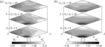
. The conditional mean production rates of the streamwise and vertical SGS stress components are shown in figure 6(a–d); the spanwise production component has trends qualitatively similar to that of the streamwise component and therefore is not included. Figure 6(b,d) shows that, for negative
 $u_{3}^{r}$
fluctuations (downdrafts),
 $\langle -(2/3){\it\tau}_{kk}\unicode[STIX]{x1D61A}_{11}|\boldsymbol{u}^{r}\rangle$
(and
 $\langle -(2/3){\it\tau}_{kk}\unicode[STIX]{x1D61A}_{22}|\boldsymbol{u}^{r}\rangle$
) are negative and
 $\langle -(2/3){\it\tau}_{kk}\unicode[STIX]{x1D61A}_{33}|\boldsymbol{u}^{r}\rangle$
is positive, indicating inter-component exchange (
 $\langle {\it\tau}_{11}|\boldsymbol{u}^{r}\rangle$
and
 $\langle {\it\tau}_{22}|\boldsymbol{u}^{r}\rangle$
losing energy to
 $\langle {\it\tau}_{33}|\boldsymbol{u}^{r}\rangle$
); the conditional spectral transfer (figure 6
a,c) is also weaker and negative for very intense downdrafts. However, because their magnitudes are relatively small, the effects of
 $\langle -(2/3){\it\tau}_{kk}\unicode[STIX]{x1D61A}_{{\it\alpha}{\it\alpha}}|\boldsymbol{u}^{r}\rangle$
and
 $\langle \unicode[STIX]{x1D617}_{{\it\alpha}{\it\alpha}}^{d}|\boldsymbol{u}^{r}\rangle$
on the SGS anisotropy are weak. For positive
 $u_{3}^{r}$
fluctuations (updrafts),
 $\langle -(2/3){\it\tau}_{kk}\unicode[STIX]{x1D61A}_{11}|\boldsymbol{u}^{r}\rangle$
is positive and
 $\langle -(2/3){\it\tau}_{kk}\unicode[STIX]{x1D61A}_{33}|\boldsymbol{u}^{r}\rangle$
is negative, indicating conditional energy transfer from the vertical to the horizontal velocity components; the conditional spectral transfer is also positive and much larger for
 $\langle {\it\tau}_{11}|\boldsymbol{u}^{r}\rangle$
, resulting in surface-layer anisotropy.
Conditional mean deviatoric and isotropic production of (a,b)
 $\langle {\it\tau}_{11}|\boldsymbol{u}^{r}\rangle$
and (c,d)
 $\langle {\it\tau}_{33}|\boldsymbol{u}^{r}\rangle$
; and the conditional mean (e) forward and (f) backscatter contributions of SGS TKE for the strongly convective (
 $0.8<-z/L\leqslant 1.5$
, with mean
 $-z/L=1.14$
) surface layer. (a)
 $\langle \unicode[STIX]{x1D617}_{11}^{d}|u_{1}^{r},u_{3}^{r}\rangle$
; (b)
 $\langle -(2/3){\it\tau}_{kk}\unicode[STIX]{x1D61A}_{11}|u_{1}^{r},u_{3}^{r}\rangle$
;(c)
 $\langle \unicode[STIX]{x1D617}_{33}^{d}|u_{1}^{r},u_{3}^{r}\rangle$
; (d)
 $\langle -(2/3){\it\tau}_{kk}\unicode[STIX]{x1D61A}_{33}|u_{1}^{r},u_{3}^{r}\rangle$
; (e)
 $\langle \mathscr{P}_{f}|u_{1}^{r},u_{3}^{r}\rangle$
; (f)
 $\langle \mathscr{P}_{b}|u_{1}^{r},u_{3}^{r}\rangle$
.

The forward contribution to the conditional mean transfer,
 $\langle \mathscr{P}_{f}|\boldsymbol{u}^{r}\rangle$
, and the backscatter contribution,
 $\langle \mathscr{P}_{b}|\boldsymbol{u}^{r}\rangle$
, of SGS turbulent kinetic energy (TKE) are shown in figures 6(e) and 6(f), respectively; here,
 $\mathscr{P}_{f}=(\mathscr{P}+|\mathscr{P}|)/2$
,
 $\mathscr{P}_{b}=(\mathscr{P}-|\mathscr{P}|)/2$
, and
 $\mathscr{P}=\mathscr{P}_{f}+\mathscr{P}_{b}$
(Piomelli, Yu & Adrian Reference Piomelli, Yu and Adrian1996), where
 $\mathscr{P}=\unicode[STIX]{x1D617}_{kk}/2$
is the production rate of TKE. The results show strong conditional forward transfer (
 $\mathscr{P}_{f}>|\mathscr{P}_{b}|$
) for positive
 $u_{3}^{r}$
(and
 $u_{1}^{r}$
) since the spectral transfer associated with the normal and shear strain rates is positive for updrafts, while for downdrafts there is conditional backscatter (
 $\mathscr{P}_{f}<|\mathscr{P}_{b}|$
). The backscatter contribution to the conditional mean transfer increases with
 ${\it\Lambda}_{w}/{\it\Delta}_{f}$
(decreasing filter width), consistent with the observations of Sullivan et al. (Reference Sullivan, Horst, Lenschow, Moeng and Weil2003) for the mean production. Similar to the conditional mean SGS stress, the conditional mean SGS production rate also has a non-diminishing dependence on the resolvable-scale velocity for all filter widths. Its magnitude is also non-diminishing, which is expected for the normal components of the production tensor since their sum is the spectral transfer rate, but suggests that
 $\langle \unicode[STIX]{x1D617}_{ij}|\boldsymbol{u}^{r}\rangle$
has a strong influence on the resolvable-scale velocity JPDF even for inertial-range filter widths.
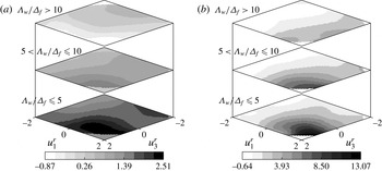
Conditional mean of the measured SGS pressure,
 $\langle p-p^{r}|u_{1}^{r},u_{3}^{r}\rangle$
, for the (a) weakly convective (
 $0<-z/L\leqslant 0.75$
, with mean
 $-z/L=0.35$
) and (b) strongly convective (
 $0.75<-z/L\leqslant 1.75$
, with mean
 $-z/L=1.31$
) surface layers.

3.2.2. Conditional mean SGS pressure
To aid our analysis of the conditional mean SGS pressure–strain-rate correlation, we present the results for the conditional mean SGS pressure,
 $\langle p-p^{r}|\boldsymbol{u}^{r}\rangle$
, in figure 7 for the weakly and strongly convective surface layers. Due to the limited amount of pressure data available, the mean (weight-averaged) values of the stability parameter here differ from those of the conditional mean SGS production since the number of datasets is reduced. The results show that
 $\langle p-p^{r}|\boldsymbol{u}^{r}\rangle$
is strongly dependent on both the streamwise and vertical components of the resolvable-scale velocity. It is generally positive (negative) for negative (positive)
 $u_{3}^{r}$
fluctuations, the former due to the deceleration of the mixed-layer eddies as they approach the ground. It also increases with
 $u_{1}^{r}$
and its dependence on
 $u_{1}^{r}$
is enhanced by negative
 $u_{3}^{r}$
and weakened by positive
 $u_{3}^{r}$
. In neutral boundary layers, such dependence has been attributed to the coherent structures generally found in turbulent boundary layer flows (Robinson Reference Robinson1991): strong positive pressure fluctuations associated with negative
 $u_{3}^{r}$
and positive
 $u_{1}^{r}$
are due to large-scale sweeps of high-velocity fluid downward toward the wall, while strong negative pressure fluctuations associated with positive
 $u_{3}^{r}$
and negative
 $u_{1}^{r}$
are likely due to ejections of low-momentum fluid upward away from the wall.
In convective surface layers, the large convective eddies have dominant contributions to the horizontal velocity fluctuations, resulting in similar but stronger trends for negative
 $u_{3}^{r}$
fluctuations. For positive
 $u_{3}^{r}$
fluctuations, strong temperature fluctuations in thermal plumes generate low-pressure regions and hence negative values of
 $\langle p-p^{r}|\boldsymbol{u}^{r}\rangle$
near the surface, which are enhanced by negative
 $u_{1}^{r}$
fluctuations (smaller
 $u_{1}^{r}$
). The magnitude of
 $\langle p-p^{r}|\boldsymbol{u}^{r}\rangle$
increases with
 $-z/L$
since the characteristic length scales of the convective eddies increase with unstable stratification, resulting in a larger fluctuating pressure field and stronger pressure reflections from the image velocity field. Recall here that the convective atmospheric surface layer is characterized by small regions of intense buoyancy-driven updrafts surrounded by broader regions of downdrafts caused by the large convective eddies of the size of the boundary layer depth (Kaimal et al.
Reference Kaimal, Wyngaard, Haugen, Coté, Izumi, Caughey and Readings1976; Lenschow & Stephens Reference Lenschow and Stephens1980; Wilczak & Tillman Reference Wilczak and Tillman1980; Khanna & Brasseur Reference Khanna and Brasseur1997). The trends of
 $\langle p-p^{r}|\boldsymbol{u}^{r}\rangle$
for the strongly convective surface layer are generally similar to those of the weakly convective ABL. For the former, the results show much stronger positive pressure fluctuations compared to negative pressure events, suggesting much stronger large-scale vertical eddy compression during downdrafts compared to relatively weaker eddy stretching during updrafts, therefore resulting in broader regions of coherent positive pressure fluctuations at the wall. As the filter width decreases, the dependence of the SGS pressure on
 $u_{3}^{r}$
generally weakens since the smaller SGS eddies (those with length scales smaller than the measurement height) are less likely to be affected by the wall (Elliott Reference Elliott1972).
3.2.3. Conditional mean SGS pressure–strain-rate correlation
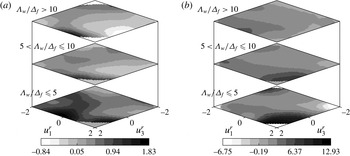
The streamwise and vertical components of the conditional mean SGS pressure–strain-rate tensor,
 $\langle \mathscr{R}_{11}|\boldsymbol{u}^{r}\rangle$
and
 $\langle \mathscr{R}_{33}|\boldsymbol{u}^{r}\rangle$
, are shown in figures 8 and 9. Nguyen et al. (Reference Nguyen, Horst, Oncley and Tong2013) previously showed that, for weakly convective surface layers, the streamwise component of the mean SGS pressure–strain-rate tensor,
 $\langle \mathscr{R}_{11}\rangle$
, is negative for all filter scales. This is expected since, for these surface layers, energy from the mean flow is fed to the subgrid scales through
 $\langle \unicode[STIX]{x1D617}_{11}\rangle$
and redistributed to
 $\langle {\it\tau}_{22}\rangle$
and
 $\langle {\it\tau}_{33}\rangle$
through
 $\langle \mathscr{R}_{ij}\rangle$
. Figure 8(a,b) shows
 $\langle \mathscr{R}_{11}|\boldsymbol{u}^{r}\rangle <0$
and
 $\langle \mathscr{R}_{33}|\boldsymbol{u}^{r}\rangle >0$
for most values of
 $u_{1}^{r}$
and
 $u_{3}^{r}$
, indicating conditional energy redistribution from the streamwise to the vertical velocity component through pressure-strain interaction. Recall that, for small values of
 $-z/L$
,
 $\langle {\it\tau}_{11}|\boldsymbol{u}^{r}\rangle$
is much larger than
 $\langle {\it\tau}_{33}|\boldsymbol{u}^{r}\rangle$
and
 $\langle \unicode[STIX]{x1D617}_{11}|\boldsymbol{u}^{r}\rangle$
is much larger than
 $\langle \unicode[STIX]{x1D617}_{33}|\boldsymbol{u}^{r}\rangle$
and
 $\langle \unicode[STIX]{x1D617}_{B33}|\boldsymbol{u}^{r}\rangle$
; therefore, the redistribution is consistent with return to isotropy. The weaker rate of pressure redistribution for negative
 $u_{3}^{r}$
reflects the wall blocking effect (hereinafter, we use this term to refer to the restriction of the vertical-velocity fluctuations): during downdrafts, the wall blocking results in a reduction of the wall-normal SGS velocity component and the rate of redistribution. The pressure fluctuations reflecting from the wall (due to the image velocity field or the image Green’s function), on the other hand, can enhance the rate of redistribution, as was alluded to by Hanjalić & Jakirlić (Reference Hanjalić, Jakirlić, Launder and Sandham2002). The wall blocking effect, however, is likely to be stronger. Thus, for the weakly convective surface layer, the effect of the wall is to dampen the rate of conditional energy redistribution from
 $\langle {\it\tau}_{11}|\boldsymbol{u}^{r}\rangle$
to
 $\langle {\it\tau}_{22}|\boldsymbol{u}^{r}\rangle$
and
 $\langle {\it\tau}_{33}|\boldsymbol{u}^{r}\rangle$
through
 $\langle \mathscr{R}_{ij}|\boldsymbol{u}^{r}\rangle$
, therefore weakening the rate of return to isotropy. The magnitude of
 $\langle \mathscr{R}_{ij}|\boldsymbol{u}^{r}\rangle$
also decreases with increasing
 ${\it\Lambda}_{w}/{\it\Delta}_{f}$
due to the isotropization of the SGS stress with decreasing filter width.
(a) The streamwise,
 $\langle \mathscr{R}_{11}|u_{1}^{r},u_{3}^{r}\rangle$
, and (b) vertical,
 $\langle \mathscr{R}_{33}|u_{1}^{r},u_{3}^{r}\rangle$
, components of the conditional mean SGS pressure–strain-rate correlation for the weakly convective (
 $0<-z/L\leqslant 0.75$
, with mean
 $-z/L=0.35$
) surface layer.

(a) The streamwise,
 $\langle \mathscr{R}_{11}|u_{1}^{r},u_{3}^{r}\rangle$
, and (b) vertical,
 $\langle \mathscr{R}_{33}|u_{1}^{r},u_{3}^{r}\rangle$
, components of the conditional mean SGS pressure–strain-rate correlation for the strongly convective (
 $0.75<-z/L\leqslant 1.75$
, with mean
 $-z/L=1.31$
) surface layer.

For moderately and strongly convective surface layers, the results show that energy is also fed to
 $\langle {\it\tau}_{33}|\boldsymbol{u}^{r}\rangle$
through buoyant production and pressure transport (discussed in § 3.2.4). Nguyen et al. (Reference Nguyen, Horst, Oncley and Tong2013) have shown that, for sufficiently convective surface layers, the mean pressure–strain-rate tensor
 $\langle \mathscr{R}_{ij}\rangle$
has a non-monotonic dependence on the filter width: while return to isotropy dominates for small filter widths,
 $\langle \mathscr{R}_{ij}\rangle$
causes SGS anisotropy for large filter widths. For these surface layers, figure 9 shows that
 $\langle \mathscr{R}_{11}|\boldsymbol{u}^{r}\rangle$
and
 $\langle \mathscr{R}_{33}|\boldsymbol{u}^{r}\rangle$
are negatively and positively correlated with
 $u_{3}^{r}$
, respectively, and that their magnitudes generally increase with
 $|u_{3}^{r}|$
. For positive
 $u_{3}^{r}$
fluctuations (updrafts),
 $\langle \mathscr{R}_{11}|\boldsymbol{u}^{r}\rangle$
is negative and
 $\langle \mathscr{R}_{33}|\boldsymbol{u}^{r}\rangle$
positive, indicating conditional energy redistribution from
 $\langle {\it\tau}_{11}|\boldsymbol{u}^{r}\rangle$
to
 $\langle {\it\tau}_{33}|\boldsymbol{u}^{r}\rangle$
through pressure–strain-rate interaction. The rate of this inter-component exchange increases with (positive)
 $u_{3}^{r}$
owing to stronger vertical stretching of the integral-scale eddies, resulting in a larger conditional energy transfer rate from the horizontal to the vertical velocity component.
For negative
 $u_{3}^{r}$
fluctuations,
 $\langle \mathscr{R}_{11}|\boldsymbol{u}^{r}\rangle$
is positive and
 $\langle \mathscr{R}_{33}|\boldsymbol{u}^{r}\rangle$
is negative (for negative
 $u_{1}^{r}$
), indicating conditional energy redistribution from
 $\langle {\it\tau}_{33}|\boldsymbol{u}^{r}\rangle$
to
 $\langle {\it\tau}_{11}|\boldsymbol{u}^{r}\rangle$
(although there are some positive values of
 $\langle \mathscr{R}_{33}|\boldsymbol{u}^{r}\rangle$
for positive
 $u_{1}^{r}$
, which are probably due to the one-sided finite-difference approximation of the vertical derivative). The results thus show that
 $\langle \mathscr{R}_{ij}|\boldsymbol{u}^{r}\rangle$
generates anisotropy due to the near-wall positive SGS pressure fluctuations found in the stagnation region within downdrafts. We note that if the updrafts were identical to downdrafts (but with reversed velocity), the stagnation region would also contain positive SGS pressure fluctuations and the contributions to
 $\langle \mathscr{R}_{{\it\alpha}{\it\alpha}}\rangle$
from both updrafts and downdrafts would cancel each other. The negative values of
 $\langle \mathscr{R}_{33}\rangle$
and positive values of
 $\langle \mathscr{R}_{11}\rangle$
(and
 $\langle \mathscr{R}_{22}\rangle$
) are therefore primarily a consequence of the updrafts and downdrafts being asymmetric. The role played by the wall blocking effect within this mechanism is to impede the vertical-velocity fluctuations, thus enhancing anisotropy. In the meantime, the pressure reflected from the surface acts to augment the pressure fluctuations and therefore is likely to enhance anisotropy (but unlikely to be the main cause of it). Thus, unlike the weakly convective (shear-dominated) surface layer, where the wall blocking and pressure reflections have opposite effects, here both act to enhance anisotropy. The contribution from the downward flow dominates the evolution of the (unconditional) mean SGS stress and therefore causes generation of anisotropy through the mean SGS pressure–strain-rate correlation, as was previously alluded to by Nguyen et al. (Reference Nguyen, Horst, Oncley and Tong2013).
The above-mentioned effects are, moreover, enhanced by convective instability (since buoyancy is more dominant, and therefore the convective eddies are more energetic) and weakened as the filter width decreases since the wall contribution diminishes for very small filter widths, and the effects of return to isotropy, although also weakening in absolute terms, becomes relatively more important (Nguyen et al.
Reference Nguyen, Horst, Oncley and Tong2013). For very small filter widths (
 ${\it\Lambda}_{w}/{\it\Delta}_{f}>10$
), there is an eventual reversal of the direction of energy exchange (
 $\langle {\it\tau}_{33}|\boldsymbol{u}^{r}\rangle$
now receiving from
 $\langle {\it\tau}_{11}|\boldsymbol{u}^{r}\rangle$
, regardless of the value of
 $u_{3}^{r}$
) and the role of
 $\langle \mathscr{R}_{ij}|\boldsymbol{u}^{r}\rangle$
for these filter widths is similar to that for the weakly convective surface layer (i.e. return to isotropy).
The dependence of
 $\langle \mathscr{R}_{22}|\boldsymbol{u}^{r}\rangle$
on
 $u_{3}^{r}$
is less apparent due to larger scatter in the computed statistics and therefore is not shown here. However, our previous analysis of
 $\langle \mathscr{R}_{22}\rangle$
has shown that the spanwise component of the mean pressure–strain-rate correlation is qualitatively similar to that of the vertical component for the weakly convective surface layer (
 $\langle {\it\tau}_{22}\rangle$
receiving energy from
 $\langle {\it\tau}_{11}\rangle$
) and to that of the streamwise component for moderately and strongly convective surface layers (
 $\langle {\it\tau}_{22}\rangle$
receiving energy from
 $\langle {\it\tau}_{33}\rangle$
). Similarly, based on the budgets of
 $\langle {\it\tau}_{11}|\boldsymbol{u}^{r}\rangle$
and
 $\langle {\it\tau}_{33}|\boldsymbol{u}^{r}\rangle$
, we can infer that the behavior of
 $\langle \mathscr{R}_{22}|\boldsymbol{u}^{r}\rangle$
is probably similar to that of
 $\langle \mathscr{R}_{33}|\boldsymbol{u}^{r}\rangle$
for the near-neutral surface layer (conditional energy redistribution from
 $\langle {\it\tau}_{11}|\boldsymbol{u}^{r}\rangle$
to
 $\langle {\it\tau}_{22}|\boldsymbol{u}^{r}\rangle$
). For strongly convective surface layers, its behaviour is likely to be similar to that of
 $\langle \mathscr{R}_{11}|\boldsymbol{u}^{r}\rangle$
.
3.2.4. Conditional mean SGS pressure transport
Previous analyses of the (unconditional) mean SGS stress by Nguyen et al. (Reference Nguyen, Horst, Oncley and Tong2013) showed that the SGS pressure transport is a major source of energy in the budget of
 $\langle {\it\tau}_{33}\rangle$
(and, therefore, a major source of energy in the budget of the mean SGS TKE), with magnitudes comparable to those inferred in the literature (Wyngaard & Coté Reference Wyngaard and Coté1971; McBean & Elliott Reference McBean and Elliott1975; Bradley, Antonia & Chambers Reference Bradley, Antonia and Chambers1981; Wilczak & Businger Reference Wilczak and Businger1984). The results for the conditional mean SGS pressure transport,
 $\langle \partial \unicode[STIX]{x1D61B}_{333}^{(p)}/\partial x_{3}|\boldsymbol{u}^{r}\rangle$
, shown in figure 10, however, indicate that it can be both a source and a sink of energy in the evolution of
 $\langle {\it\tau}_{33}|\boldsymbol{u}^{r}\rangle$
. It is generally small for weakly convective surface layers (figure 10
a), except for large filter widths, for which it is a gain and generally increases with
 $u_{3}^{r}$
. For strongly convective surface layers (figure 10
b) and large filter widths,
 $\langle \partial \unicode[STIX]{x1D61B}_{333}^{(p)}/\partial x_{3}|\boldsymbol{u}^{r}\rangle$
is the dominant source of energy for
 $\langle {\it\tau}_{33}|\boldsymbol{u}^{r}\rangle$
for positive
 $u_{3}^{r}$
(since energy is imported downward from higher
 $z$
by pressure work) and a small loss for negative
 $u_{3}^{r}$
. For small filter widths, the pressure transport is generally weak for negative
 $u_{3}^{r}$
and a gain for positive
 $u_{3}^{r}$
, depending weakly on
 $u_{1}^{r}$
. The results for positive
 $u_{3}^{r}$
fluctuations suggest that the conditional mean pressure transport may be driven by the negative local pressure minima which follow large-scale updrafts (figure 7). The physics associated with negative SGS pressure transport for negative
 $u_{3}^{r}$
fluctuations, however, is unclear and warrants further study.
Conditional mean SGS pressure transport of
 $\langle {\it\tau}_{33}|\boldsymbol{u}^{r}\rangle$
,
 $\langle \partial \unicode[STIX]{x1D61B}_{333}^{(p)}/\partial x_{3}|u_{1}^{r},u_{3}^{r}\rangle$
, for the (a) weakly convective (
 $0<-z/L\leqslant 0.3$
, with mean
 $-z/L=0.23$
) and (b) strongly convective (
 $1<-z/L\leqslant 2.5$
, with mean
 $-z/L=1.83$
) surface layers.

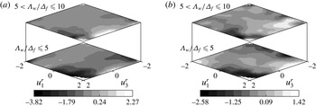
3.2.5. Conditional mean SGS turbulent transport
The conditional mean turbulent transport of
 $\langle {\it\tau}_{11}|\boldsymbol{u}^{r}\rangle$
and
 $\langle {\it\tau}_{33}|\boldsymbol{u}^{r}\rangle$
, shown in figure 11 for the strongly convective surface layer, is generally negative for positive
 $u_{3}^{r}$
fluctuations, indicating upward transport of TKE. It is small for negative
 $u_{3}^{r}$
fluctuations. Its magnitude generally decreases with the filter width and increases with
 $-z/L$
due to the stronger thermal plumes which are characteristic of the highly convective surface layer. The results also show that the magnitude and dependence of
 $\langle \partial \unicode[STIX]{x1D61B}_{11k}^{(t)}/\partial x_{k}|\boldsymbol{u}^{r}\rangle$
on
 $\boldsymbol{u}^{r}$
are generally similar to those of
 $\langle \partial \unicode[STIX]{x1D61B}_{33k}^{(t)}/\partial x_{k}|\boldsymbol{u}^{r}\rangle$
, indicating that the conditional mean turbulent transport is nearly isotropic and therefore has a weak influence on the anisotropy of the conditional mean SGS stress. Its magnitude is also relatively small compared to the other budget terms, therefore making
 $\langle \partial \unicode[STIX]{x1D61B}_{{\it\alpha}{\it\alpha}k}^{(t)}/\partial x_{k}|\boldsymbol{u}^{r}\rangle$
a relatively minor source of SGS energy. We note that the mean (weight-averaged) values of the stability parameter in figure 11 are slightly higher than those for the previous figures since calculation of the turbulent transport requires data from the upwind sonic anemometer array (for the streamwise derivative) and therefore reduces the number of usable datasets (from 26 to 18) since we require that both the upwind- and downwind-array measurements meet quality thresholds.
Conditional mean SGS turbulent transport of (a)
 $\langle {\it\tau}_{11}|\boldsymbol{u}^{r}\rangle$
,
 $\langle \partial \unicode[STIX]{x1D61B}_{11k}^{(t)}/\partial x_{k}|u_{1}^{r},u_{3}^{r}\rangle$
, and (b)
 $\langle {\it\tau}_{33}|\boldsymbol{u}^{r}\rangle$
,
 $\langle \partial \unicode[STIX]{x1D61B}_{33k}^{(t)}/\partial x_{k}|u_{1}^{r},u_{3}^{r}\rangle$
, for the strongly convective (
 $1.5<-z/L\leqslant 2.5$
, with mean
 $-z/L=2.1$
) surface layer.

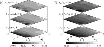
3.2.6. Advection of the conditional mean SGS stress
The vertical advection of
 $\langle {\it\tau}_{11}|\boldsymbol{u}^{r}\rangle$
and
 $\langle {\it\tau}_{33}|\boldsymbol{u}^{r}\rangle$
in physical space, shown in figure 12, is a major source (for negative
 $u_{3}^{r}$
) and sink (for positive
 $u_{3}^{r}$
) of energy in the budgets of the conditional mean SGS stress. For negative
 $u_{3}^{r}$
fluctuations, both
 $-v_{3}\partial \langle {\it\tau}_{11}|\boldsymbol{u}^{r}\rangle /\partial x_{3}$
and
 $-v_{3}\partial \langle {\it\tau}_{33}|\boldsymbol{u}^{r}\rangle /\partial x_{3}$
are positive, indicating gains by
 $\langle {\it\tau}_{11}|\boldsymbol{u}^{r}\rangle$
and
 $\langle {\it\tau}_{33}|\boldsymbol{u}^{r}\rangle$
due to downward advection of SGS TKE. For positive
 $u_{3}^{r}$
fluctuations, the advection terms are negative, indicating losses by
 $\langle {\it\tau}_{11}|\boldsymbol{u}^{r}\rangle$
and
 $\langle {\it\tau}_{33}|\boldsymbol{u}^{r}\rangle$
due to upward advection of SGS energy. The energy loss due to upward advection is comparable in magnitude to the conditional mean shear production (for
 $\langle {\it\tau}_{11}|\boldsymbol{u}^{r}\rangle$
) and the conditional mean pressure transport (for
 $\langle {\it\tau}_{33}|\boldsymbol{u}^{r}\rangle$
), both of which are the major budget gains during updrafts. However, because it has similar effects on both
 $\langle {\it\tau}_{11}|\boldsymbol{u}^{r}\rangle$
and
 $\langle {\it\tau}_{33}|\boldsymbol{u}^{r}\rangle$
,
 $-v_{3}\partial \langle {\it\tau}_{{\it\alpha}{\it\alpha}}|\boldsymbol{u}^{r}\rangle /\partial x_{3}$
does not contribute significantly to the SGS anisotropy. Advection of the conditional mean SGS stress in velocity space due to the resolvable-scale acceleration (second term in (1.1); not shown) is negligible, while the remaining budget term representing the covariance of the conditional mean fluctuations of the SGS stress and the conditional mean resolvable-scale acceleration is prohibitively difficult to compute and therefore omitted here.
Vertical advection of (a)
 $\langle {\it\tau}_{11}|\boldsymbol{u}^{r}\rangle$
,
 $-v_{3}\partial \langle {\it\tau}_{11}|u_{1}^{r},u_{3}^{r}\rangle /\partial x_{3}$
, and (b)
 $\langle {\it\tau}_{33}|\boldsymbol{u}^{r}\rangle$
,
 $-v_{3}\partial \langle {\it\tau}_{33}|u_{1}^{r},u_{3}^{r}\rangle /\partial x_{3}$
, for the strongly convective (
 $0.8<-z/L\leqslant 1.5$
, with mean
 $-z/L=1.14$
) surface layer.

3.2.7. Conditional mean SGS shear stress budget
Similar to
 $\langle {\it\tau}_{13}\rangle$
, the evolution of
 $\langle {\it\tau}_{13}|\boldsymbol{u}^{r}\rangle$
is dominated by the conditional mean shear production, buoyant production and velocity–pressure-gradient correlation. The conditional mean turbulent transport is small, while viscous dissipation is negligible due to local isotropy. The total production rate of
 $\langle {\it\tau}_{13}|\boldsymbol{u}^{r}\rangle$
,
 $\langle \unicode[STIX]{x1D617}_{13}+\unicode[STIX]{x1D617}_{B13}|\boldsymbol{u}^{r}\rangle$
, is shown in figure 13. (Although production of
 $\langle {\it\tau}_{13}|\boldsymbol{u}^{r}\rangle$
due to shear exceeds production due to buoyancy, both
 $\langle \unicode[STIX]{x1D617}_{13}|\boldsymbol{u}^{r}\rangle$
and
 $\langle \unicode[STIX]{x1D617}_{B13}|\boldsymbol{u}^{r}\rangle$
follow the trends shown in figure 13.) The results show that
 $\langle \unicode[STIX]{x1D617}_{13}+\unicode[STIX]{x1D617}_{B13}|\boldsymbol{u}^{r}\rangle$
is negative, indicating production of
 $\langle {\it\tau}_{13}|\boldsymbol{u}^{r}\rangle$
since the shear stress is negative. Its magnitude generally increases with
 $\boldsymbol{u}^{r}$
and
 $-z/L$
. The results for
 $\langle \unicode[STIX]{x1D617}_{13}|\boldsymbol{u}^{r}\rangle$
in terms of the contributions from the deviatoric and isotropic parts of the SGS stress (
 $\unicode[STIX]{x1D617}_{13}^{d}$
and
 $-(2/3){\it\tau}_{kk}\unicode[STIX]{x1D61A}_{13}$
, respectively; not shown) indicate that the former is positive, indicating destruction of the conditional mean SGS shear stress due to the straining and rotation of the anisotropic part of the SGS turbulence, while the latter is negative with nearly twice the magnitude, indicating production of
 $\langle {\it\tau}_{13}|\boldsymbol{u}^{r}\rangle$
due to the straining of the isotropic part of the SGS turbulence. Here,
 $\langle -(2/3){\it\tau}_{kk}\unicode[STIX]{x1D61A}_{13}|\boldsymbol{u}^{r}\rangle$
decreases in magnitude with increasing
 ${\it\Lambda}_{w}/{\it\Delta}_{f}$
(decreasing filter width) as the interaction between
 $\langle {\it\tau}_{kk}\rangle$
and the shear strain weaken, while
 $\langle \unicode[STIX]{x1D617}_{13}^{d}|\boldsymbol{u}^{r}\rangle$
also decreases with
 ${\it\Lambda}_{w}/{\it\Delta}_{f}$
since
 $\langle {\it\tau}_{ij}|\boldsymbol{u}^{r}\rangle$
is less anisotropic.
Sum of the conditional mean shear production and conditional mean buoyant production rates of
 $\langle {\it\tau}_{13}|\boldsymbol{u}^{r}\rangle$
,
 $\langle \unicode[STIX]{x1D617}_{13}+\unicode[STIX]{x1D617}_{B13}|u_{1}^{r},u_{3}^{r}\rangle$
, for the (a) weakly convective (
 $0<-z/L\leqslant 0.8$
, with mean
 $-z/L=0.35$
) and (b) strongly convective (
 $0.8<-z/L\leqslant 1.5$
, with mean
 $-z/L=1.14$
) surface layers.

The conditional mean SGS velocity–pressure-gradient correlation,
 $\langle {\it\Pi}_{13}|\boldsymbol{u}^{r}\rangle$
, which includes both the effects of the conditional mean pressure destruction and the conditional mean pressure transport of
 $\langle {\it\tau}_{13}|\boldsymbol{u}^{r}\rangle$
, is shown in figure 14. The results show that
 $\langle {\it\Pi}_{13}|\boldsymbol{u}^{r}\rangle$
is positive for both weakly and strongly convective surface layers and all filter widths, indicating destruction of the conditional mean SGS shear stress. Similar to
 $\langle \unicode[STIX]{x1D617}_{13}|\boldsymbol{u}^{r}\rangle$
and
 $\langle \unicode[STIX]{x1D617}_{B13}|\boldsymbol{u}^{r}\rangle$
,
 $\langle {\it\Pi}_{13}|\boldsymbol{u}^{r}\rangle$
increases in magnitude with
 $u_{1}^{r}$
and
 $u_{3}^{r}$
. Its dependence on
 $\boldsymbol{u}^{r}$
weakens with
 ${\it\Lambda}_{w}/{\it\Delta}_{f}$
since the resolvable-scale velocity has a diminishing effect on the smaller SGS eddies. The results for the conditional mean pressure–strain-rate correlation and the conditional mean pressure transport show that the former is dominant, with trends similar to
 $\langle {\it\Pi}_{13}|\boldsymbol{u}^{r}\rangle$
. We note that the trends and magnitude of
 $\langle {\it\Pi}_{13}|\boldsymbol{u}^{r}\rangle$
generally counter those of the conditional mean shear and buoyant production for both weakly and strongly convective surface layers and all filter widths, indicating that the conditional mean velocity–pressure-gradient correlation plays the usual role of causing return to isotropy in the evolution of
 $\langle {\it\tau}_{13}|\boldsymbol{u}^{r}\rangle$
. The weaker rate of pressure destruction for negative
 $u_{3}^{r}$
also indicates that the wall blocking effect merely dampens the rate of return to isotropy. The conditional mean advection (not shown) is positive (a sink) during updrafts and small during downdrafts, with magnitudes much smaller than the conditional mean production and pressure destruction.
Conditional mean SGS velocity–pressure-gradient correlation in the transport equation of
 $\langle {\it\tau}_{13}|\boldsymbol{u}^{r}\rangle$
,
 $\langle {\it\Pi}_{13}|u_{1}^{r},u_{3}^{r}\rangle$
, for the (a) weakly convective (
 $0<-z/L\leqslant 0.75$
, with mean
 $-z/L=0.23$
) and (b) strongly convective (
 $1.75<-z/L\leqslant 2.5$
, with mean
 $-z/L=1.83$
) surface layers.

3.3. Conditional mean SGS temperature flux budget
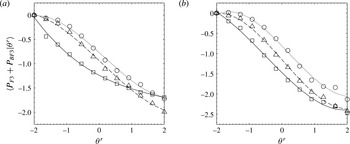
The conditional mean production rates of the horizontal and vertical components of the SGS potential temperature flux are shown in figures 15 and 16, respectively; we note that the non-dimensionalized flux production terms shown have opposite signs relative to the actual flux production since
 $T_{\ast }<0$
for unstable surface layers. The results show that
 $\langle \unicode[STIX]{x1D617}_{F1}|{\it\theta}^{r}\rangle$
is positive and
 $\langle P_{F3}+P_{BF3}|{\it\theta}^{r}\rangle$
is negative (indicating production of
 $\langle F_{1}|{\it\theta}^{r}\rangle$
and
 $\langle F_{3}|{\it\theta}^{r}\rangle$
, respectively), both increasing in magnitude with
 ${\it\theta}^{r}$
. Although the production rate of
 $\langle F_{3}|{\it\theta}^{r}\rangle$
due to stratification (
 $\langle P_{F3}|{\it\theta}^{r}\rangle$
) exceeds production due to buoyancy (
 $\langle P_{BF3}|{\it\theta}^{r}\rangle$
) for the weakly convective surface layer, both generally follow the trends shown in figure 16. For positive
 ${\it\theta}^{r}$
fluctuations, the eddies associated with updrafts generally come from near the ground and therefore carry larger amounts of vertical SGS heat flux and SGS stress. They are also likely to have experienced stronger shear and vertical temperature gradient, both of which were shown to be the dominant contributions to
 $\langle P_{\mathit{Fi}}\rangle$
(Chen et al.
Reference Chen, Liu and Tong2010). For negative
 ${\it\theta}^{r}$
fluctuations, the eddies associated with downdrafts generally come from the mixed layer and carry relatively small amounts of SGS heat flux and SGS stress (buoyant production is also smaller); therefore,
 $\langle P_{\mathit{Fi}}|{\it\theta}^{r}\rangle$
(and
 $\langle P_{BF3}|{\it\theta}^{r}\rangle$
) are smaller.
Conditional mean production of SGS horizontal temperature flux for the (a) weakly convective (
 $0<-z/L\leqslant 1$
, with mean
 $-z/L=0.45$
) and (b) strongly convective (
 $1<-z/L\leqslant 2.5$
, with mean
 $-z/L=1.70$
) surface layers and varying values of the wavelength–filter-width ratio: ▫,
 ${\it\Lambda}_{w}/{\it\Delta}_{f}\leqslant 5$
; ▵,
 $5<{\it\Lambda}_{w}/{\it\Delta}_{f}\leqslant 10$
;○,
 ${\it\Lambda}_{w}/{\it\Delta}_{f}>10$
.

Conditional mean production of SGS vertical temperature flux for the (a) weakly convective (
 $0<-z/L\leqslant 1$
, with mean
 $-z/L=0.45$
) and (b) strongly convective (
 $1<-z/L\leqslant 2.5$
, with mean
 $-z/L=1.70$
) surface layers. The data are grouped as in figure 15.

The magnitudes of
 $\langle P_{\mathit{Fi}}|{\it\theta}^{r}\rangle$
also decrease with increasing
 ${\it\Lambda}_{w}/{\it\Delta}_{f}$
because the SGS velocity and scalar are more isotropic for smaller filter widths (isotropy implies vanishing heat flux). For small filter widths, the dependence of
 $\langle P_{F1}|{\it\theta}^{r}\rangle$
on
 ${\it\theta}^{r}$
also weakens for negative temperature fluctuations (downdrafts) since the SGS flux carried by the returning downflow is likely to be well-mixed; this is less the case for positive temperature fluctuations (updrafts). As
 $-z/L$
increases, the conditional mean production rate of
 $\langle F_{1}|{\it\theta}^{r}\rangle$
decreases (for large filter widths) because the turbulence field is increasingly isotropic in the horizontal plane, resembling that of local free convection. The dependence of
 $\langle P_{F1}|{\it\theta}^{r}\rangle$
on
 $z/L$
is weaker for larger values of
 ${\it\Lambda}_{w}/{\it\Delta}_{f}$
because, for these filter widths, the SGS flux is already quite isotropic (the effects of buoyancy are also weaker). Similar filter-width dependence is shown for
 $\langle P_{F3}|{\it\theta}^{r}\rangle$
. As
 $-z/L$
increases, however,
 $\langle P_{F3}|{\it\theta}^{r}\rangle$
, when non-dimensionalized using surface-layer scaling, should increase to a constant value since
 $\langle F_{3}|{\it\theta}^{r}\rangle$
is produced at a nearly constant rate in the free convection limit (Wyngaard, Coté & Izumi Reference Wyngaard, Coté and Izumi1971). However, since
 $\langle P_{BF3}|{\it\theta}^{r}\rangle$
increases with
 $-z/L$
,
 $\langle P_{F3}+P_{BF3}|{\it\theta}^{r}\rangle$
also increases slowly with
 $-z/L$
.
Conditional mean SGS pressure–temperature-gradient correlation in the budget of
 $\langle F_{1}|{\it\theta}^{r}\rangle$
for the (a) weakly convective (
 $0<-z/L\leqslant 1$
, with mean
 $-z/L=0.45$
) and (b) strongly convective (
 $1<-z/L\leqslant 2.5$
, with mean
 $-z/L=1.70$
) surface layers. The data are grouped as in figure 15.

Conditional mean SGS temperature–pressure-gradient correlation in the budget of
 $\langle F_{3}|{\it\theta}^{r}\rangle$
for the (a) weakly convective (
 $0<-z/L\leqslant 1$
, with mean
 $-z/L=0.45$
) and (b) strongly convective (
 $1<-z/L\leqslant 2.5$
, with mean
 $-z/L=1.70$
) surface layers. The data are grouped as in figure 15.

The horizontal and vertical components of the conditional mean temperature–pressure-gradient correlation are shown in figures 17 and 18, respectively. Assuming nominal horizontal homogeneity of the field site, the pressure transport of
 $\langle F_{1}|{\it\theta}^{r}\rangle$
is small and hence
 $\langle {\it\Pi}_{F1}|{\it\theta}^{r}\rangle$
is dominated by the conditional mean SGS pressure–temperature-gradient correlation
 $\langle \mathscr{R}_{F1}|{\it\theta}^{r}\rangle$
, which we show in place of
 $\langle {\it\Pi}_{F1}|{\it\theta}^{r}\rangle$
. Figure 17 shows that
 $\langle \mathscr{R}_{F1}|{\it\theta}^{r}\rangle$
is negative for both weakly and strongly convective surface layers and all filter widths, indicating destruction of
 $\langle F_{1}|{\it\theta}^{r}\rangle$
; its trends and magnitude generally balance those of
 $\langle P_{F1}|{\it\theta}^{r}\rangle$
(the advection and turbulent transport, not shown, are both small). Similar to the flux production rate, its magnitude increases with increasing
 ${\it\theta}^{r}$
and
 ${\it\Delta}_{f}$
(decreasing
 ${\it\Lambda}_{w}/{\it\Delta}_{f}$
) since the scalar field anisotropy increases with the vertical shear and filter scale. As the filter width decreases,
 $\langle \mathscr{R}_{F1}|{\it\theta}^{r}\rangle$
weakens since the smaller SGS eddies are less anisotropic, therefore the tendency of
 $\langle \mathscr{R}_{F1}|{\it\theta}^{r}\rangle$
to drive the conditional mean flux towards isotropy weakens. It also decreases with increasing
 $-z/L$
since the scalar field is more horizontally isotropic as local free convection scaling is approached. Figure 18 shows that
 $\langle {\it\Pi}_{F3}|{\it\theta}^{r}\rangle$
(which includes the conditional mean SGS pressure transport and the conditional mean SGS pressure–temperature-gradient correlation) is positive for both weakly and strongly convective surface layers and all filter widths, indicating destruction of
 $\langle F_{3}|{\it\theta}^{r}\rangle$
. Similar to the vertical SGS temperature flux production rate, its magnitude increases with increasing
 ${\it\theta}^{r}$
and decreases with decreasing filter width. It also increases asymptotically with
 $-z/L$
to a constant (local free convection) rate. Although the trends of
 $\langle {\it\Pi}_{F3}|{\it\theta}^{r}\rangle$
generally counter those of
 $\langle P_{F3}+P_{BF3}|{\it\theta}^{r}\rangle$
, its measured magnitude is considerably smaller than the total production rate, perhaps due to the attenuation of the fluctuating vertical pressure gradient by the finite difference scheme. Its trends, however, suggest that
 $\langle {\it\Pi}_{F3}|{\it\theta}^{r}\rangle$
plays the usual role of causing return to isotropy in the budget of
 $\langle F_{3}|{\it\theta}^{r}\rangle$
.
Schematics summarizing the conditional energy transfer during (a) updrafts and (b) downdrafts for the strongly convective surface layer and large filter widths. Solid and dashed arrows represent major and minor energy transfer (in relative magnitudes), respectively. The sizes of the circles containing
 ${\it\tau}_{11}$
and
 ${\it\tau}_{33}$
indicate their relative magnitudes. An arrow pointing towards (away from) a circle represents a source (sink). Because the pressure transport and turbulent transport are relatively weak and contain larger scatter for
 $u_{3}^{r}<0$
, we omit their contributions in (b).

3.4. Combined effects of the budget terms on the conditional mean SGS stress
The above results show that the budgets of the normal components of the conditional mean SGS stress are much more complex than those of the conditional mean SGS shear stress and SGS temperature flux, which are simply dominated by the conditional mean production and the pressure destruction. The budget of
 $\langle {\it\tau}_{11}|\boldsymbol{u}^{r}\rangle$
is dominated by the conditional mean production, the pressure–strain-rate correlation and the turbulent transport, while that of
 $\langle {\it\tau}_{33}|\boldsymbol{u}^{r}\rangle$
also includes the conditional mean buoyant production and the pressure transport. To summarize the effects of the budget terms on the SGS stress structure, we show in figure 19 schematics of the conditional energy transfer during updrafts and downdrafts. A summary of the energy balance is given below.
When
 $u_{3}^{r}$
(and
 $u_{1}^{r}$
) are positive,
 $\langle {\it\tau}_{11}|\boldsymbol{u}^{r}\rangle$
receives large amounts of energy from the resolvable scales through the conditional mean shear production. Meanwhile,
 $\langle {\it\tau}_{33}|\boldsymbol{u}^{r}\rangle$
receives energy from the buoyant production, the pressure–strain-rate correlation and the pressure transport, with the last term serving as the dominant source of SGS energy for positive
 $u_{3}^{r}$
fluctuations. The conditional mean advection and, to a lesser extent, the conditional mean turbulent transport move much of this energy to higher
 $z$
, while the pressure–strain-rate correlation redistributes relatively small amounts of energy from
 $\langle {\it\tau}_{11}|\boldsymbol{u}^{r}\rangle$
to
 $\langle {\it\tau}_{33}|\boldsymbol{u}^{r}\rangle$
. The conditional redistribution part of the production tensor removes relatively small amounts of energy from
 $\langle {\it\tau}_{33}|\boldsymbol{u}^{r}\rangle$
. Because the conditional mean advection has similar effects on both
 $\langle {\it\tau}_{11}|\boldsymbol{u}^{r}\rangle$
and
 $\langle {\it\tau}_{33}|\boldsymbol{u}^{r}\rangle$
, it does not contribute significantly to the SGS anisotropy. However, due to the large gains by
 $\langle {\it\tau}_{11}|\boldsymbol{u}^{r}\rangle$
through shear production, the resulting SGS stress structure for positive
 $u_{3}^{r}$
and
 $u_{1}^{r}$
is anisotropic with one large eigenvalue. As
 $u_{1}^{r}$
decreases,
 $\langle {\it\tau}_{ij}|\boldsymbol{u}^{r}\rangle$
remains anisotropic but transitions toward a one small eigenvalue structure since
 $\langle \unicode[STIX]{x1D617}_{11}|\boldsymbol{u}^{r}\rangle$
(although still larger than
 $\langle \unicode[STIX]{x1D617}_{33}|\boldsymbol{u}^{r}\rangle$
) is relatively weaker (compared to its magnitude for positive
 $u_{1}^{r}$
) and more comparable in magnitude to
 $\langle \unicode[STIX]{x1D617}_{22}|\boldsymbol{u}^{r}\rangle$
.
When
 $u_{3}^{r}$
is negative, the magnitudes of the budget terms are smaller due to generally weaker spectral transfer (and hence weaker production). Here,
 $\langle {\it\tau}_{11}|\boldsymbol{u}^{r}\rangle$
receives SGS energy from
 $\langle {\it\tau}_{33}|\boldsymbol{u}^{r}\rangle$
through the pressure–strain-rate correlation, contrary to return to isotropy. Meanwhile, both components receive a significant amount of energy through advection. Again, because the conditional mean advection has similar effects on both
 $\langle {\it\tau}_{11}|\boldsymbol{u}^{r}\rangle$
and
 $\langle {\it\tau}_{33}|\boldsymbol{u}^{r}\rangle$
, it does not contribute significantly to the SGS anisotropy. Additionally,
 $\langle {\it\tau}_{11}|\boldsymbol{u}^{r}\rangle$
loses a small amount of energy to
 $\langle {\it\tau}_{33}|\boldsymbol{u}^{r}\rangle$
through the conditional redistribution part of the production tensor, while spectral transfer is small for both components (for very intense downdrafts, there is conditional backscatter). The conditional mean buoyant production, turbulent transport and pressure transport are also weak, and therefore the magnitude of
 $\langle {\it\tau}_{33}|\boldsymbol{u}^{r}\rangle$
is smaller. Because both
 $\langle {\it\tau}_{11}|\boldsymbol{u}^{r}\rangle$
and
 $\langle {\it\tau}_{33}|\boldsymbol{u}^{r}\rangle$
and their budget terms are smaller, the conditional mean SGS stress is much less anisotropic for negative
 $u_{3}^{r}$
.
The dominant SGS energy balance in the convective atmospheric surface layer is therefore as follows. Shear production and pressure transport provide energy (the former to
 $\langle {\it\tau}_{11}|\boldsymbol{u}^{r}\rangle$
and the latter to
 $\langle {\it\tau}_{33}|\boldsymbol{u}^{r}\rangle$
) during updrafts. Advection, meanwhile, removes much of this energy to higher
 $z$
. During downdrafts, energy is advected downward (from higher
 $z$
) back to both components. At the same time, the pressure–strain-rate correlation redistributes the energy from
 $\langle {\it\tau}_{33}|\boldsymbol{u}^{r}\rangle$
to
 $\langle {\it\tau}_{11}|\boldsymbol{u}^{r}\rangle$
(which is relatively larger), causing strong SGS anisotropy. Dissipation, although not measured, is expected to be active and relatively isotropic. Using the current dataset, Nguyen et al. (Reference Nguyen, Horst, Oncley and Tong2013) have shown that the budgets of the (unconditional) mean SGS stress and mean SGS temperature flux are approximately satisfied. In balancing the budgets of the normal components of the mean SGS stress, they approximated the mean dissipation rate using functional forms given in the literature (e.g. Caughey & Wyngaard Reference Caughey and Wyngaard1979). In the present study, since the (conditional) dissipation rate was not measured, it is not possible to quantify the balance of the budgets of the normal components of the conditional mean SGS stress. However, for the conditional mean SGS shear stress (where dissipation is negligible due to local isotropy) and the conditional mean SGS temperature flux (where there is no dissipation), the conditional production is approximately balanced by the conditional pressure destruction (when their magnitudes are interpolated to comparable
 $z/L$
), and therefore the budgets for these components appear to be satisfied. As stated previously, the imbalance of the vertical scalar flux budget may be due to the attenuation of the fluctuating vertical pressure gradient by the finite difference scheme.
4. Discussion and conclusions
Turbulence measurement data obtained in the convective atmospheric surface layer during the AHATS field campaign were used to study the conditional mean SGS stress and the conditional mean SGS potential temperature flux. The field program notably includes measurements of the fluctuating pressure, therefore allowing for the budgets of the second-order SGS turbulence moments to be obtained. We showed that the terms which evolve the budgets of the conditional mean SGS stress and the conditional mean SGS temperature flux must be correctly predicted by the SGS model in order for LES to reproduce the resolvable-scale velocity JPDF and the resolvable-scale temperature PDF. We analysed the dependence of the budget terms on the surface-layer stability and filter width and showed that they are closely related to the dynamics of the convective atmospheric surface layer; more specifically, when conditioned on the resolvable-scale velocity, the budget terms show a strong dependence on the updrafts generated by buoyancy, downdrafts associated with the returning flow of convective eddies, and wall blocking effects. The results provide new insights into the SGS physics first educed in the previous study of the mean budget terms by Nguyen et al. (Reference Nguyen, Horst, Oncley and Tong2013), particularly those involving the SGS pressure.
The present study shows that the budgets of the normal components of the conditional mean SGS stress are most complex for the strongly convective surface layer and large filter widths, where the conditional mean shear and buoyant production, advection in physical space, pressure transport, pressure–strain-rate interaction and dissipation play an active role. During updrafts, the conditional mean shear production and the conditional mean pressure transport are the dominant sources of SGS energy (the former for
 $\langle {\it\tau}_{11}|\boldsymbol{u}^{r}\rangle$
and the latter for
 $\langle {\it\tau}_{33}|\boldsymbol{u}^{r}\rangle$
), while the conditional mean advection and dissipation are the dominant sinks for both. During downdrafts, the conditional mean advection, which feeds back to
 $\langle {\it\tau}_{11}|\boldsymbol{u}^{r}\rangle$
and
 $\langle {\it\tau}_{33}|\boldsymbol{u}^{r}\rangle$
much of the energy taken from them during updrafts, is the dominant source for the latter. Much of the energy gained by
 $\langle {\it\tau}_{33}|\boldsymbol{u}^{r}\rangle$
from advection is transferred to
 $\langle {\it\tau}_{11}|\boldsymbol{u}^{r}\rangle$
by the conditional mean pressure–strain-rate correlation. Meanwhile, dissipation is a sink for both components. It is notable that the pressure transport is large only during updrafts, considering that much of the energy transfer from
 $\langle {\it\tau}_{33}|\boldsymbol{u}^{r}\rangle$
to
 $\langle {\it\tau}_{11}|\boldsymbol{u}^{r}\rangle$
through the pressure–strain-rate correlation occurs during downdrafts. The role played by the conditional mean advection is also notable given that advection of the (unconditional) mean SGS stress vanishes in a horizontally homogeneous ABL.
The results for the conditional mean SGS pressure–strain-rate correlation show that the normal components of
 $\langle \mathscr{R}_{ij}|\boldsymbol{u}^{r}\rangle$
have more complex behaviours in strongly convective surface layers than in weakly convective ones due to the role played by strong updrafts, downdrafts and wall effects. For weakly convective surface layers and large filter widths, much of the conditional energy transfer from the resolvable to the subgrid scales is first fed primarily to the streamwise velocity component and subsequently redistributed to the remaining (spanwise and vertical) components by the conditional mean pressure–strain-rate correlation, consistent with return to isotropy. For these surface layers, the role played by
 $\langle \mathscr{R}_{ij}|\boldsymbol{u}^{r}\rangle$
in the budget of the conditional mean SGS stress is similar to that of
 $\langle \mathscr{R}_{ij}\rangle$
in the budget of the (unconditional) mean SGS stress. For the former, we show that wall blockage of the vertical-velocity fluctuations during downdrafts dampens the rate of conditional energy redistribution. As the filter scale decreases, conditional mean production for the spanwise and vertical components becomes significant and the conditional mean SGS stress is likely to be more isotropic. Here, the role of
 $\langle \mathscr{R}_{ij}|\boldsymbol{u}^{r}\rangle$
diminishes, much like that of
 $\langle \mathscr{R}_{ij}\rangle$
in the budget of the mean SGS stress.
The behaviour of the conditional mean SGS pressure–strain-rate correlation for moderately and strongly convective surface layers is qualitatively different from that of the weakly convective surface layer. For these surface layers,
 $\langle \mathscr{R}_{ij}|\boldsymbol{u}^{r}\rangle$
redistributes energy from the (larger) horizontal to the (smaller) vertical velocity component during updrafts, probably due to stronger vertical stretching of the energy-containing eddies. During downdrafts, however, it redistributes SGS energy in the opposite direction (i.e. from the smaller vertical to the larger horizontal velocity components) and is the main cause of surface-layer SGS anisotropy, contrary to its commonly recognized role. The results also show that the conditional mean SGS pressure is generally positive for negative
 $u_{3}^{r}$
and vice versa. Because of the asymmetry between the SGS pressure within updrafts and downdrafts, however, generation of SGS anisotropy is due to the positive SGS pressure fluctuations associated with the returning downflow of the convective eddies. The role played by the wall blocking effect and wall pressure reflection within this mechanism is to enhance the anisotropy, but the latter is unlikely to be the main cause of anisotropy. The results substantiate the importance of wall effects on the evolution of the (unconditional) mean SGS stress, for which the pressure–strain-rate correlation is the primary cause of anisotropy (Nguyen et al.
Reference Nguyen, Horst, Oncley and Tong2013). These effects, however, weaken with decreasing filter width since the effects of the wall are reduced. For very small filter widths, the effects of return to isotropy become relatively more important and the role of
 $\langle \mathscr{R}_{ij}|\boldsymbol{u}^{r}\rangle$
is similar to that for the weakly convective surface layer (i.e. causing return to isotropy).
In contrast, the role of the conditional mean SGS velocity–pressure-gradient correlation in the budget of the conditional mean SGS shear stress and that of the conditional mean SGS temperature–pressure-gradient correlation in the budget of the conditional mean SGS temperature flux are qualitatively similar for both weakly and strongly convective surface layers; that is, they act to counter the conditional mean production. The roles played by these terms are analogous to those of their unconditioned counterparts in the budgets of the mean SGS shear stress and mean SGS temperature flux.
The results also show that the pressure transport of TKE is relatively small for weakly convective surface layers, while for strongly convective surface layers it can be both a source and a sink of SGS energy, depending strongly on the resolvable-scale vertical velocity. It is positive for positive
 $u_{3}^{r}$
fluctuations and vice versa, the former suggesting that the import of TKE into the surface layer by the pressure work is likely to be due to the negative local pressure minima which follow large-scale updrafts. The behaviour of the pressure transport for downdrafts, however, remains unclear and warrants further study.
The conditional analyses in the present work have important implications for SGS models, particularly models of the near-wall SGS pressure–strain-rate correlation. A common approach to modelling the pressure–strain-rate correlation in Reynolds-averaged Navier Stokes (RANS) parameterizations is to split the term into three parts (slow, rapid and wall blocking (e.g. Pope Reference Pope2000)) using the Green’s function solution to the Poisson equation (Chou Reference Chou1945) and to model each part separately. The slow and rapid parts promote energy redistribution as a means of reducing the anisotropy of the Reynolds stress and the Reynolds stress production tensors (e.g. Naot, Shavit & Wolfshtein Reference Naot, Shavit and Wolfshtein1970), respectively, whereas the wall blocking part dampens the rate of redistribution (e.g. Gibson & Launder Reference Gibson and Launder1978). The slow part is almost always modelled using Rotta’s return-to-isotropy model (Rotta Reference Rotta1951). In the present study, the approximate balance between the SGS production and the SGS pressure destruction in the budgets of the conditional mean SGS shear stress and those of the conditional mean SGS heat flux for both weakly and strongly convective surface layers and all filter widths indicates that the pressure plays the expected role of causing return to isotropy, consistent with models for the slow and rapid pressure–strain-rate correlation. Similar behaviour for the normal components of
 $\langle \mathscr{R}_{ij}|\boldsymbol{u}^{r}\rangle$
for the weakly convective surface layer suggests that they can be modelled using conventional return-to-isotropy models, as is done in Ramachandran & Wyngaard (Reference Ramachandran and Wyngaard2011). Smaller magnitudes of
 $\langle \mathscr{R}_{ij}|\boldsymbol{u}^{r}\rangle$
observed for negative
 $u_{3}^{r}$
reflect the wall blocking effect, and can be properly modelled using existing wall damping models. These models, however, are unable to correctly predict the near-wall behaviour of the pressure–strain-rate correlation in the moderately and strongly convective surface layers, where the sign of
 $\langle \mathscr{R}_{ij}|\boldsymbol{u}^{r}\rangle$
is reversed during downdrafts. Because this effect is most significant for large filter widths, new models for both the Reynolds and SGS pressure–strain-rate correlation that can properly reflect the near-wall dynamics of the convective boundary layer, as revealed in the present study, are needed.
Acknowledgements
We thank Professor J. Wyngaard at Penn State University and Drs P. Sullivan, T. Horst, S. Oncley, and W. Brown at NCAR for their collaboration in the AHATS field campaign. This work was supported by the National Science Foundation through grant no. ATM-1335995.
Appendix A. Derivation of the transport equations for
 $\langle {\it\tau}_{ij}|\boldsymbol{u}^{r}\rangle$
and
$\langle F_{i}|{\it\theta}^{r}\rangle$


The transport equation governing the evolution of the conditional mean is derived below using the delta-function technique (e.g. Pope Reference Pope2000, Reference Pope2010) for given quantity
 $\boldsymbol{Q}(\boldsymbol{x},t)$
and conditioning variables
 $\boldsymbol{C}(\boldsymbol{x},t)$
. Denoting the JPDF of
 $\boldsymbol{C}(\boldsymbol{x},t)$
by
 $$\begin{eqnarray}f_{c}(\boldsymbol{c};t)=\langle {\it\delta}(\boldsymbol{C}(\boldsymbol{x},t)-\boldsymbol{c})\rangle ,\end{eqnarray}$$
the conditional mean of
 $\boldsymbol{Q}(\boldsymbol{x},t)$
,
 $\langle \boldsymbol{Q}|\boldsymbol{C}=\boldsymbol{c}\rangle$
, is given by
 $$\begin{eqnarray}f_{c}(\boldsymbol{c};t)\langle \boldsymbol{Q}(\boldsymbol{x},t)|\boldsymbol{C}(\boldsymbol{x},t)=\boldsymbol{c}\rangle =\langle \boldsymbol{Q}(\boldsymbol{x},t){\it\delta}(\boldsymbol{C}(\boldsymbol{x},t)-\boldsymbol{c})\rangle ,\end{eqnarray}$$
where
 $\langle \boldsymbol{Q}|\boldsymbol{C}=\boldsymbol{c}\rangle$
denotes the mean value of
 $\boldsymbol{Q}$
given that
 $\boldsymbol{C}$
takes the value
 $\boldsymbol{c}$
. Differentiating both sides of (A 2) with respect to
 $x_{i}$
yields
 $$\begin{eqnarray}\displaystyle f_{c}\frac{\partial \langle \boldsymbol{Q}|\boldsymbol{c}\rangle }{\partial x_{i}}+\frac{\partial f_{c}}{\partial x_{i}}\langle \boldsymbol{Q}|\boldsymbol{c}\rangle & = & \displaystyle \left\langle \frac{\partial \boldsymbol{Q}}{\partial x_{i}}{\it\delta}(\boldsymbol{C}-\boldsymbol{c})\right\rangle +\left\langle \boldsymbol{Q}\frac{\partial {\it\delta}(\boldsymbol{C}-\boldsymbol{c})}{\partial x_{i}}\right\rangle \nonumber\\ \displaystyle & = & \displaystyle f_{c}\left\langle \frac{\partial \boldsymbol{Q}}{\partial x_{i}}|\boldsymbol{c}\right\rangle +\left\langle \boldsymbol{Q}\frac{\partial {\it\delta}(\boldsymbol{C}-\boldsymbol{c})}{\partial \boldsymbol{C}}\frac{\partial \boldsymbol{C}}{\partial x_{i}}\right\rangle \nonumber\\ \displaystyle & = & \displaystyle f_{c}\left\langle \frac{\partial \boldsymbol{Q}}{\partial x_{i}}|\boldsymbol{c}\right\rangle -\frac{\partial }{\partial \boldsymbol{c}}\left\langle \boldsymbol{Q}{\it\delta}(\boldsymbol{C}-\boldsymbol{c})\frac{\partial \boldsymbol{C}}{\partial x_{i}}\right\rangle ,\end{eqnarray}$$
and therefore
 $$\begin{eqnarray}\left\langle \frac{\partial \boldsymbol{Q}}{\partial x_{i}}|\boldsymbol{c}\right\rangle =\frac{\partial \langle \boldsymbol{Q}|\boldsymbol{c}\rangle }{\partial x_{i}}+\frac{1}{f_{c}}\frac{\partial f_{c}}{\partial x_{i}}\langle \boldsymbol{Q}|\boldsymbol{c}\rangle +\frac{1}{f_{c}}\frac{\partial }{\partial \boldsymbol{c}}\left[\left\langle \boldsymbol{Q}\frac{\partial \boldsymbol{C}}{\partial x_{i}}|\boldsymbol{c}\right\rangle f_{c}\right].\end{eqnarray}$$
For
 $\boldsymbol{Q}=1$
, (A 4) reduces to
 $$\begin{eqnarray}\frac{\partial f_{c}}{\partial x_{i}}=-\frac{\partial }{\partial \boldsymbol{c}}\left[\left\langle \frac{\partial \boldsymbol{C}}{\partial x_{i}}|\boldsymbol{c}\right\rangle f_{c}\right].\end{eqnarray}$$
From (A 4) and (A 5), we obtain
 $$\begin{eqnarray}\displaystyle \left\langle \frac{\partial \boldsymbol{Q}}{\partial x_{i}}|\boldsymbol{c}\right\rangle & = & \displaystyle \frac{\partial \langle \boldsymbol{Q}|\boldsymbol{c}\rangle }{\partial x_{i}}-\frac{1}{f_{c}}\frac{\partial }{\partial \boldsymbol{c}}\left[\left\langle \frac{\partial \boldsymbol{C}}{\partial x_{i}}|\boldsymbol{c}\right\rangle f_{c}\right]\langle \boldsymbol{Q}|\boldsymbol{c}\rangle +\frac{1}{f_{c}}\frac{\partial }{\partial \boldsymbol{c}}\left[\left\langle \boldsymbol{Q}\frac{\partial \boldsymbol{C}}{\partial x_{i}}|\boldsymbol{c}\right\rangle f_{c}\right]\nonumber\\ \displaystyle & = & \displaystyle \frac{\partial \langle \boldsymbol{Q}|\boldsymbol{c}\rangle }{\partial x_{i}}+\left\langle \frac{\partial \boldsymbol{C}}{\partial x_{i}}|\boldsymbol{c}\right\rangle \frac{\partial \langle \boldsymbol{Q}|\boldsymbol{c}\rangle }{\partial \boldsymbol{c}}+\frac{1}{f_{c}}\frac{\partial }{\partial \boldsymbol{c}}\left[\text{cov}\left(\boldsymbol{Q},\frac{\partial \boldsymbol{C}}{\partial x_{i}}|\boldsymbol{c}\right)f_{c}\right],\end{eqnarray}$$
where
 $$\begin{eqnarray}\text{cov}\left(\boldsymbol{Q},\frac{\partial \boldsymbol{C}}{\partial x_{i}}|\boldsymbol{c}\right)=\left\langle \boldsymbol{Q}\frac{\partial \boldsymbol{C}}{\partial x_{i}}|\boldsymbol{c}\right\rangle -\left\langle \boldsymbol{Q}|\boldsymbol{c}\right\rangle \left\langle \frac{\partial \boldsymbol{C}}{\partial x_{i}}|\boldsymbol{c}\right\rangle\end{eqnarray}$$
is the conditional covariance between
 $\boldsymbol{Q}$
and
 $\partial \boldsymbol{C}/\partial x_{i}$
.
Similarly, differentiating both sides of (A 2) with respect to
 $t$
yields
 $$\begin{eqnarray}f_{c}\frac{\partial \langle \boldsymbol{Q}|\boldsymbol{c}\rangle }{\partial t}+\frac{\partial f_{c}}{\partial t}\langle \boldsymbol{Q}|\boldsymbol{c}\rangle =f_{c}\left\langle \frac{\partial \boldsymbol{Q}}{\partial t}|\boldsymbol{c}\right\rangle -\frac{\partial }{\partial \boldsymbol{c}}\left\langle \boldsymbol{Q}{\it\delta}(\boldsymbol{C}-\boldsymbol{c})\frac{\partial \boldsymbol{C}}{\partial t}\right\rangle\end{eqnarray}$$
and, after manipulations similar to (A 4)–(A 6), we obtain
 $$\begin{eqnarray}\frac{\partial \langle \boldsymbol{Q}|\boldsymbol{c}\rangle }{\partial t}=\left\langle \frac{\partial \boldsymbol{Q}}{\partial t}|\boldsymbol{c}\right\rangle -\left\langle \frac{\partial \boldsymbol{C}}{\partial t}|\boldsymbol{c}\right\rangle \frac{\partial \langle \boldsymbol{Q}|\boldsymbol{c}\rangle }{\partial \boldsymbol{c}}-\frac{1}{f_{c}}\frac{\partial }{\partial \boldsymbol{c}}\left[\text{cov}\left(\boldsymbol{Q},\frac{\partial \boldsymbol{C}}{\partial t}|\boldsymbol{c}\right)f_{c}\right].\end{eqnarray}$$
A.1. Transport equation for
$\langle {\it\tau}_{ij}|\boldsymbol{u}^{r}\rangle$

Using (A 9) with
 $\boldsymbol{Q}={\it\tau}_{ij}$
,
 $\boldsymbol{C}=\boldsymbol{u}^{r}$
(with the sample-space variable
 $\boldsymbol{c}=\boldsymbol{v}$
), and
 $\partial {\it\tau}_{ij}/\partial t$
given by (e.g. Lilly Reference Lilly and Goldstine1967)
 $$\begin{eqnarray}\frac{\partial {\it\tau}_{ij}}{\partial t}=-u_{k}^{r}\frac{\partial {\it\tau}_{ij}}{\partial x_{k}}+\frac{\partial }{\partial x_{k}}\unicode[STIX]{x1D61B}_{ijk}^{(t)}+\unicode[STIX]{x1D617}_{ij}+\unicode[STIX]{x1D617}_{Bij}+{\it\Pi}_{ij}-{\it\epsilon}_{ij},\end{eqnarray}$$
we obtain
 $$\begin{eqnarray}\displaystyle \frac{\partial \langle {\it\tau}_{ij}|\boldsymbol{u}^{r}\rangle }{\partial t} & = & \displaystyle \left\langle \frac{\partial {\it\tau}_{ij}}{\partial t}|\boldsymbol{u}^{r}\right\rangle -\left\langle \frac{\partial u_{k}^{r}}{\partial t}|\boldsymbol{u}^{r}\right\rangle \frac{\partial \langle {\it\tau}_{ij}|\boldsymbol{u}^{r}\rangle }{\partial v_{k}}-\frac{1}{f_{u}}\frac{\partial }{\partial v_{l}}\left[\text{cov}\left({\it\tau}_{ij},\frac{\partial u_{l}^{r}}{\partial t}|\boldsymbol{u}^{r}\right)f_{u}\right]\nonumber\\ \displaystyle & = & \displaystyle \left\langle -u_{k}^{r}\frac{\partial {\it\tau}_{ij}}{\partial x_{k}}|\boldsymbol{u}^{r}\right\rangle +\left\langle \frac{\partial }{\partial x_{k}}\unicode[STIX]{x1D61B}_{ijk}^{(t)}+\unicode[STIX]{x1D617}_{ij}+\unicode[STIX]{x1D617}_{Bij}+{\it\Pi}_{ij}-{\it\epsilon}_{ij}|\boldsymbol{u}^{r}\right\rangle \nonumber\\ \displaystyle & & \displaystyle -\,\left\langle \frac{\partial u_{k}^{r}}{\partial t}|\boldsymbol{u}^{r}\right\rangle \frac{\partial \langle {\it\tau}_{ij}|\boldsymbol{u}^{r}\rangle }{\partial v_{k}}-\frac{1}{f_{u}}\frac{\partial }{\partial v_{l}}\left[\text{cov}\left({\it\tau}_{ij},\frac{\partial u_{l}^{r}}{\partial t}|\boldsymbol{u}^{r}\right)f_{u}\right],\end{eqnarray}$$
where, for convenience, the sample-space variable in the conditional means has been omitted. Re-writing the conditional mean spatial derivative (first term on the right-hand side of (A 11)) using (A 6) yields
 $$\begin{eqnarray}\displaystyle \frac{\partial \langle {\it\tau}_{ij}|\boldsymbol{u}^{r}\rangle }{\partial t} & = & \displaystyle -v_{k}\left\{\frac{\partial \langle {\it\tau}_{ij}|\boldsymbol{u}^{r}\rangle }{\partial x_{k}}+\left\langle \frac{\partial u_{l}^{r}}{\partial x_{k}}|\boldsymbol{u}^{r}\right\rangle \frac{\partial \langle {\it\tau}_{ij}|\boldsymbol{u}^{r}\rangle }{\partial v_{l}}+\frac{1}{f_{u}}\frac{\partial }{\partial v_{l}}\left[\text{cov}\left({\it\tau}_{ij},\frac{\partial u_{l}^{r}}{\partial x_{k}}|\boldsymbol{u}^{r}\right)f_{u}\right]\right\}\nonumber\\ \displaystyle & & \displaystyle +\,\left\langle \frac{\partial }{\partial x_{k}}\unicode[STIX]{x1D61B}_{ijk}^{(t)}+\unicode[STIX]{x1D617}_{ij}+\unicode[STIX]{x1D617}_{Bij}+{\it\Pi}_{ij}-{\it\epsilon}_{ij}|\boldsymbol{u}^{r}\right\rangle \nonumber\\ \displaystyle & & \displaystyle -\,\left\langle \frac{\partial u_{k}^{r}}{\partial t}|\boldsymbol{u}^{r}\right\rangle \frac{\partial \langle {\it\tau}_{ij}|\boldsymbol{u}^{r}\rangle }{\partial v_{k}}-\frac{1}{f_{u}}\frac{\partial }{\partial v_{l}}\left[\text{cov}\left({\it\tau}_{ij},\frac{\partial u_{l}^{r}}{\partial t}|\boldsymbol{u}^{r}\right)f_{u}\right].\end{eqnarray}$$
Here,
 $u_{k}^{r}$
takes the value
 $v_{k}$
and is taken out of the conditional mean. Re-arrangement of (A 12) yields the transport equation for
 $\langle {\it\tau}_{ij}|\boldsymbol{u}^{r}\rangle$
,
 $$\begin{eqnarray}\displaystyle \frac{\partial \left\langle {\it\tau}_{ij}|\boldsymbol{u}^{r}\right\rangle }{\partial t} & = & \displaystyle -v_{k}\frac{\partial \left\langle {\it\tau}_{ij}|\boldsymbol{u}^{r}\right\rangle }{\partial x_{k}}-\left\langle \left(\frac{\partial u_{l}^{r}}{\partial t}+u_{k}^{r}\frac{\partial u_{l}^{r}}{\partial x_{k}}\right)|\boldsymbol{u}^{r}\right\rangle \frac{\partial \left\langle {\it\tau}_{ij}|\boldsymbol{u}^{r}\right\rangle }{\partial v_{l}}\nonumber\\ \displaystyle & & \displaystyle +\,\left\langle \frac{\partial }{\partial x_{k}}\unicode[STIX]{x1D61B}_{ijk}^{(t)}|\boldsymbol{u}^{r}\right\rangle +\left\langle \unicode[STIX]{x1D617}_{ij}|\boldsymbol{u}^{r}\right\rangle +\left\langle \unicode[STIX]{x1D617}_{Bij}|\boldsymbol{u}^{r}\right\rangle +\left\langle {\it\Pi}_{ij}|\boldsymbol{u}^{r}\right\rangle -\left\langle {\it\epsilon}_{ij}|\boldsymbol{u}^{r}\right\rangle \nonumber\\ \displaystyle & & \displaystyle -\,\frac{1}{f_{u}}\frac{\partial }{\partial v_{l}}\left[\text{cov}\left({\it\tau}_{ij},\frac{\partial u_{l}^{r}}{\partial t}+u_{k}^{r}\frac{\partial u_{l}^{r}}{\partial x_{k}}|\boldsymbol{u}^{r}\right)f_{u}\right].\end{eqnarray}$$
A.2. Transport equation for
$\langle F_{i}|{\it\theta}^{r}\rangle$

Similarly, using (A 9) with
 $\boldsymbol{Q}=F_{i}$
,
 $\boldsymbol{C}={\it\theta}^{r}$
(with the sample-space variable
 $\boldsymbol{c}={\it\psi}$
), and
 $\partial F_{i}/\partial t$
given by
 $$\begin{eqnarray}\frac{\partial F_{i}}{\partial t}=-u_{k}^{r}\frac{\partial F_{i}}{\partial x_{k}}+\frac{\partial }{\partial x_{k}}\unicode[STIX]{x1D61B}_{Fik}^{(t)}+P_{\mathit{Fi}}+P_{BFi}+{\it\Pi}_{\mathit{Fi}},\end{eqnarray}$$
we obtain
 $$\begin{eqnarray}\displaystyle \frac{\partial \langle F_{i}|{\it\theta}^{r}\rangle }{\partial t} & = & \displaystyle \left\langle \frac{\partial F_{i}}{\partial t}|{\it\theta}^{r}\right\rangle -\left\langle \frac{\partial {\it\theta}^{r}}{\partial t}|{\it\theta}^{r}\right\rangle \frac{\partial \langle F_{i}|{\it\theta}^{r}\rangle }{\partial {\it\psi}}-\frac{1}{f_{{\it\theta}}}\frac{\partial }{\partial {\it\psi}}\left[\text{cov}\left(F_{i},\frac{\partial {\it\theta}^{r}}{\partial t}|{\it\theta}^{r}\right)f_{{\it\theta}}\right]\nonumber\\ \displaystyle & = & \displaystyle \left\langle -u_{k}^{r}\frac{\partial F_{i}}{\partial x_{k}}|{\it\theta}^{r}\right\rangle +\left\langle \frac{\partial }{\partial x_{k}}\unicode[STIX]{x1D61B}_{Fik}^{(t)}+P_{\mathit{Fi}}+P_{BFi}+{\it\Pi}_{\mathit{Fi}}|{\it\theta}^{r}\right\rangle \nonumber\\ \displaystyle & & \displaystyle -\,\left\langle \frac{\partial {\it\theta}^{r}}{\partial t}|{\it\theta}^{r}\right\rangle \frac{\partial \langle F_{i}|{\it\theta}^{r}\rangle }{\partial {\it\psi}}-\frac{1}{f_{{\it\theta}}}\frac{\partial }{\partial {\it\psi}}\left[\text{cov}\left(F_{i},\frac{\partial {\it\theta}^{r}}{\partial t}|{\it\theta}^{r}\right)f_{{\it\theta}}\right],\end{eqnarray}$$
where, again, the sample-space variable in the conditional means has been omitted for convenience. The first term on the right-hand side of (A 15) can be expressed as
 $$\begin{eqnarray}\left\langle -u_{k}^{r}\frac{\partial F_{i}}{\partial x_{k}}|{\it\theta}^{r}\right\rangle =-\left\langle u_{k}^{r}|{\it\theta}^{r}\right\rangle \left\langle \frac{\partial F_{i}}{\partial x_{k}}|{\it\theta}^{r}\right\rangle -\text{cov}\left(u_{k}^{r},\frac{\partial F_{i}}{\partial x_{k}}|{\it\theta}^{r}\right).\end{eqnarray}$$
Re-writing the conditional mean spatial derivative using (A 6) yields
 $$\begin{eqnarray}\displaystyle \frac{\partial \langle F_{i}|{\it\theta}^{r}\rangle }{\partial t} & = & \displaystyle -\left\langle u_{k}^{r}|{\it\theta}^{r}\right\rangle \!\left\{\frac{\partial \langle F_{i}|{\it\theta}^{r}\rangle }{\partial x_{k}}+\left\langle \frac{\partial {\it\theta}^{r}}{\partial x_{k}}|{\it\theta}^{r}\!\right\rangle \!\frac{\partial \langle F_{i}|{\it\theta}^{r}\rangle }{\partial {\it\psi}}+\frac{1}{f_{{\it\theta}}}\frac{\partial }{\partial {\it\psi}}\!\left[\text{cov}\!\left(F_{i},\frac{\partial {\it\theta}^{r}}{\partial x_{k}}|{\it\theta}^{r}\right)f_{{\it\theta}}\right]\right\}\nonumber\\ \displaystyle & & \displaystyle -\,\text{cov}\left(u_{k}^{r},\frac{\partial F_{i}}{\partial x_{k}}|{\it\theta}^{r}\right)+\left\langle \frac{\partial }{\partial x_{k}}\unicode[STIX]{x1D61B}_{Fik}^{(t)}+P_{\mathit{Fi}}+P_{BFi}+{\it\Pi}_{\mathit{Fi}}|{\it\theta}^{r}\right\rangle \nonumber\\ \displaystyle & & \displaystyle -\,\left\langle \frac{\partial {\it\theta}^{r}}{\partial t}|{\it\theta}^{r}\right\rangle \frac{\partial \langle F_{i}|{\it\theta}^{r}\rangle }{\partial {\it\psi}}-\frac{1}{f_{{\it\theta}}}\frac{\partial }{\partial {\it\psi}}\left[\text{cov}\left(F_{i},\frac{\partial {\it\theta}^{r}}{\partial t}|{\it\theta}^{r}\right)f_{{\it\theta}}\right].\end{eqnarray}$$
Re-arranging (A 17) yields the transport equation for
 $\langle F_{i}|{\it\theta}^{r}\rangle$
,
 $$\begin{eqnarray}\displaystyle \frac{\partial \left\langle F_{i}|{\it\theta}^{r}\right\rangle }{\partial t} & = & \displaystyle -\left\{\left\langle u_{k}^{r}|{\it\theta}^{r}\right\rangle \frac{\partial \left\langle F_{i}|{\it\theta}^{r}\right\rangle }{\partial x_{k}}+\text{cov}\left(u_{k}^{r},\frac{\partial F_{i}}{\partial x_{k}}|{\it\theta}^{r}\right)\right\}\nonumber\\ \displaystyle & & \displaystyle -\,\left\langle \left(\frac{\partial {\it\theta}^{r}}{\partial t}+\left\langle u_{k}^{r}|{\it\theta}^{r}\right\rangle \frac{\partial {\it\theta}^{r}}{\partial x_{k}}\right)|{\it\theta}^{r}\right\rangle \frac{\partial \left\langle F_{i}|{\it\theta}^{r}\right\rangle }{\partial {\it\psi}}\nonumber\\ \displaystyle & & \displaystyle +\,\left\langle \frac{\partial }{\partial x_{k}}\unicode[STIX]{x1D61B}_{Fik}^{(t)}|{\it\theta}^{r}\right\rangle +\left\langle P_{\mathit{Fi}}|{\it\theta}^{r}\right\rangle +\left\langle P_{BFi}|{\it\theta}^{r}\right\rangle +\left\langle {\it\Pi}_{\mathit{Fi}}|{\it\theta}^{r}\right\rangle \nonumber\\ \displaystyle & & \displaystyle -\,\frac{1}{f_{{\it\theta}}}\frac{\partial }{\partial {\it\psi}}\left[\text{cov}\left(F_{i},\frac{\partial {\it\theta}^{r}}{\partial t}+\left\langle u_{k}^{r}|{\it\theta}^{r}\right\rangle \frac{\partial {\it\theta}^{r}}{\partial x_{k}}|{\it\theta}^{r}\right)f_{{\it\theta}}\right].\end{eqnarray}$$