1 Introduction
A grand aim of physics is to seek simplification by distilling the most basic elements out of complex phenomena. Quantitative models can be constructed from a minimal set of postulated elements, and then tested against available empirical data. Satisfactory agreement with the data generally suggests that a certain level of physical understanding has been attained. In this spirit, we seek in this investigation to develop a simple model of the turbulent boundary layer by leveraging a body of research over the past two decades that has transformed important aspects of our understanding of such flows. Characterizations of statistical structure, in particular, now more clearly reflect the interactions across scales and the influence of increasing scale separation with increasing Reynolds number (Klewicki Reference Klewicki2010). With this improved understanding come new opportunities to more efficiently represent the basic mechanisms that underlie the observed flow properties and their Reynolds number dependencies. Specifically, we employ here a complementary set of theoretically educed and empirically observed findings to formulate a simple model for the streamwise velocity fluctuations in turbulent wall flows. In essence, this model leverages the physical space manifestation of scale separation between the momentum and vorticity fields that emerges with increasing Reynolds number in these flows.
The empirical foundation of the present model is provided by the increasingly binary spatial structure of the instantaneous spanwise vorticity field with increasing Reynolds number, as first revealed by the particle image velocimetry (PIV) measurements of Meinhart & Adrian (Reference Meinhart and Adrian1995). These authors observed that, in the outer region of the turbulent boundary layer (say
 $y/\unicode[STIX]{x1D6FF}\gtrsim 0.05$
, where
 $y$
is the coordinate normal to the wall and
 $\unicode[STIX]{x1D6FF}$
is the boundary layer thickness), there exist large-scale zones of nearly uniform streamwise (
 $x$
) momentum, which they called uniform momentum zones (UMZs). Meinhart and Adrian also observed that adjacent UMZs are separated by slender regions of intense spanwise vorticity,
 $\tilde{\unicode[STIX]{x1D714}}_{z}$
. Here,
 $\tilde{\bullet }$
denotes a total instantaneous quantity; that is,
 $\tilde{\unicode[STIX]{x1D714}}_{z}=\unicode[STIX]{x1D6FA}_{z}+\unicode[STIX]{x1D714}_{z}$
, where henceforth an uppercase variable denotes a temporal or ensemble mean and a lowercase variable represents the fluctuation about this mean. For subsequent references
 $\tilde{u}$
,
 $\tilde{v}$
, and
 $\tilde{w}$
are the total velocity components in the
 $x$
,
 $y$
and
 $z$
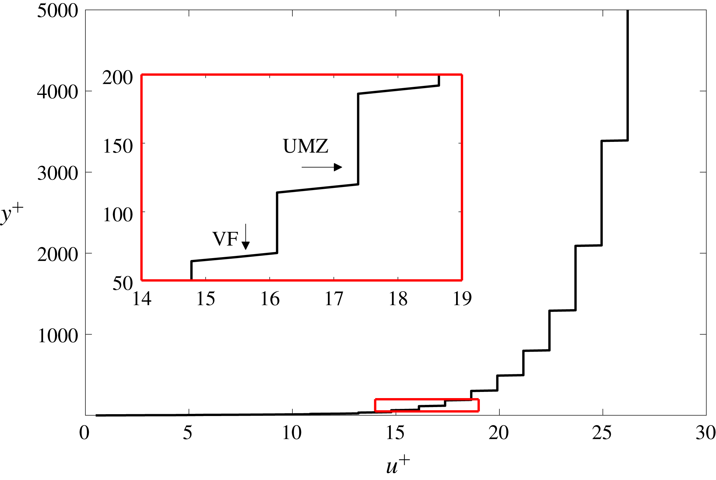
directions, respectively. Following Priyadarshana et al. (Reference Priyadarshana, Klewicki, Treat and Foss2007), we call the shear-layer-like motions vortical fissures (VFs), since the internal vorticity structure of these motions has not yet been well documented and may in fact exhibit significant Reynolds number dependence. The spatial arrangement of VFs and UMZs causes the instantaneous streamwise velocity profile to take on a staircase-like character, with most of the net velocity variation being spatially intermittent and concentrated within the VFs (Meinhart & Adrian Reference Meinhart and Adrian1995). The target of the present model is to capture essential features of the momentum transport associated with this heterogeneous structure.
Shear-layer-like interfaces and concentrated internal shear layers have long been thought to play an important role in the dynamics of turbulent flows (Corrsin & Kistler Reference Corrsin and Kistler1955; Ishihara, Kaneda & Hunt Reference Ishihara, Kaneda and Hunt2003; Westerweel et al.
Reference Westerweel, Fukushima, Pedersen and Hunt2009; Kwon et al.
Reference Kwon, Philip, deSilva, Hutchins and Monty2014; da Silva et al.
Reference da Silva, Hunt, Eames and Westerweel2014; Chauhan et al.
Reference Chauhan, Philip, deSilva, Hutchins and Marusic2014a
; Eisma et al.
Reference Eisma, Westerweel, Ooms and Elsinga2015). In an isothermal constant density viscous flow, molecular diffusion is the sole means by which irrotational fluid particles can gain vorticity. Corrsin & Kistler (Reference Corrsin and Kistler1955) leveraged this physical constraint to advance the concept of the viscous superlayer: the wrinkled sheet of viscous vortical fluid comprising the corrugated instantaneous interface at the outer edge of a turbulent shear flow. Since then, numerous studies have attempted to determine the properties associated with turbulent/non-turbulent interfaces (e.g. da Silva et al.
Reference da Silva, Hunt, Eames and Westerweel2014). Owing to the difficulties in measuring vorticity directly, with few exceptions (e.g. see Klewicki, Falco & Foss Reference Klewicki, Falco and Foss1992), most of these investigations have used thresholds on surrogate quantities, e.g. velocity magnitudes or jumps in temperature, to identify the bounding interface (Chen & Blackwelder Reference Chen and Blackwelder1978). The advent of increasingly high Reynolds number direct numerical simulations (DNS) and reasonably well-resolved PIV has allowed for estimates of the thickness of, and velocity increment across, the viscous superlayer and, similarly, the widths, velocity increments and average spacing (
 ${\approx}$
UMZ widths) of the internal shear layers (VFs) in wall-bounded flows (Adrian, Meinhart & Tomkins Reference Adrian, Meinhart and Tomkins2000; Kwon et al.
Reference Kwon, Philip, deSilva, Hutchins and Monty2014; Chauhan et al.
Reference Chauhan, Philip, deSilva, Hutchins and Marusic2014a
; Eisma et al.
Reference Eisma, Westerweel, Ooms and Elsinga2015).
The present model construction finds its firmest theoretical basis in the region where the mean viscous force in the mean momentum balance is sub-dominant, i.e. in the inertial domain. This condition is significant since it is commensurate with the VFs occupying a diminishing fraction of the overall flow volume in the limit of very large friction Reynolds number
 $\unicode[STIX]{x1D6FF}^{+}\equiv \unicode[STIX]{x1D6FF}u_{\unicode[STIX]{x1D70F}}/\unicode[STIX]{x1D708}$
, where
 $u_{\unicode[STIX]{x1D70F}}$
is the friction velocity and
 $\unicode[STIX]{x1D708}$
is the kinematic viscosity, and is physically in accord with the dominance of advective vorticity transport in that region. In contrast, the motions bearing high-amplitude vorticity in the near-wall region are nearly continuously distributed in space, i.e. spacing filling (Johansson & Alfredsson Reference Johansson and Alfredsson1991; Jimenez & Pinelli Reference Jimenez and Pinelli1999; Klewicki & Hirschi Reference Klewicki and Hirschi2004), and the vorticity field is much more strongly influenced by the mechanism of vorticity stretching (Klewicki Reference Klewicki2013b
).
Despite its simplicity, the present modelling framework implicitly reflects and explicitly incorporates a number of estimated UMZ and VF properties. Through the use of existing PIV measurements, along with threshold crossing analysis of well-resolved
 $\unicode[STIX]{x1D714}_{z}$
time series, Klewicki (Reference Klewicki2013b
) provided the first estimates of the average VF width
 $f_{w}$
as a function of
 $\unicode[STIX]{x1D6FF}^{+}$
. These planar PIV and time-series-based estimates exhibit good agreement at laboratory-scale
 $\unicode[STIX]{x1D6FF}^{+}$
, indicating that
 $f_{w}/\unicode[STIX]{x1D6FF}\approx 1.3/\sqrt{\unicode[STIX]{x1D6FF}^{+}}$
, which also approximates the Taylor microscale
 $\unicode[STIX]{x1D6EC}_{T}$
up to
 $\unicode[STIX]{x1D6FF}^{+}\approx 15\,000$
(Marusic & Adrian Reference Marusic and Adrian2010). This scaling with
 $\unicode[STIX]{x1D6EC}_{T}$
also agrees with the lower-
 $\unicode[STIX]{x1D6FF}^{+}$
 $\unicode[STIX]{x1D714}_{z}$
time series measurements of Klewicki & Falco (Reference Klewicki and Falco1996), showing that the average scale of the
 $\unicode[STIX]{x1D714}_{z}$
bearing motions on the inertial domain becomes independent of
 $y^{+}$
, and simultaneously of the detection threshold (
 ${>}{\unicode[STIX]{x1D714}_{z}}_{rms}$
), where the subscript rms refers to the root-mean-square of the fluctuations. Similarly, the recent high resolution PIV measurements of Eisma et al. (Reference Eisma, Westerweel, Ooms and Elsinga2015) at
 $\unicode[STIX]{x1D6FF}^{+}\approx 2050$
indicate that the fissure width is approximately
 $40\,\%$
of the Taylor scale across the entire outer region, a result that is essentially identical to earlier
 $\unicode[STIX]{x1D714}_{z}$
event duration analyses (Klewicki & Falco Reference Klewicki and Falco1996) and reinforced by recent PIV analyses at higher
 $\unicode[STIX]{x1D6FF}^{+}$
(de Silva et al.
Reference de Silva, Philip, Hutchins and Marusic2017). Relevant to asymptotic structure, large field-of-view PIV measurements at the Surface Layer Turbulence and Environmental Science Test (SLTEST) facility (Klewicki et al.
Reference Klewicki, Metzger, Kelner and Thurlow1995) by Morris et al. (Reference Morris, Stolpa, Slaboch and Klewicki2007) exploited the near-neutral atmospheric surface layer (ASL) to attain a very high Reynolds number condition:
 $\unicode[STIX]{x1D6FF}^{+}\approx 600\,000$
. These data not only provide further evidence that UMZs and VFs exist, but also suggest that, at these very large
 $\unicode[STIX]{x1D6FF}^{+}$
, the internal structure of the VFs is spatially complex. Thus, this VF structure is potentially different from that observed at lower Reynolds numbers, where some observations suggest that the VFs comprise a concatenation of discrete vortices (Adrian et al.
Reference Adrian, Meinhart and Tomkins2000). Owing to limitations on the spatial resolution of the measurements by Morris et al. however, the variation of the internal structure of the VFs with
 $\unicode[STIX]{x1D6FF}^{+}$
remains an open question. Nevertheless, it is intriguing that estimates of the VF thickness derived from the PIV measurements of Morris et al. also show good agreement with the
 $f_{w}/\unicode[STIX]{x1D6FF}\approx 1.3/\sqrt{\unicode[STIX]{x1D6FF}^{+}}$
dependence ascertained at lower
 $\unicode[STIX]{x1D6FF}^{+}$
. On the other hand, the vorticity time series and Taylor-scale estimates from the SLTEST site show much smaller values than
 $f_{w}/\unicode[STIX]{x1D6FF}$
as measured by PIV (Klewicki Reference Klewicki2013b
). This discrepancy between the different detection methods is consistent with the possibility that VFs develop an internal turbulence structure at sufficiently large
 $\unicode[STIX]{x1D6FF}^{+}$
.
Theoretical justification for the
 $1/\sqrt{\unicode[STIX]{x1D6FF}^{+}}$
scaling of the dimensionless fissure width comes from the mean momentum equation analysis of Klewicki (Reference Klewicki2013c
). Consistently, the inertial-layer self-sustaining process (SSP) theory of Chini et al. (Reference Chini, Montemuro, White and Klewicki2017) and its more recent revision by B. Montemuro (2018, private communication), both of which are derived directly from an asymptotic reduction of the Navier–Stokes equations, predict that the outer-normalized fissure thickness scales approximately like 1/𝛿+
2/5 and 1/𝛿+
7/16, respectively. Recent PIV measurements by de Silva, Hutchins & Marusic (Reference de Silva, Hutchins and Marusic2016) further suggest an approximately logarithmic
 $\unicode[STIX]{x1D6FF}^{+}$
-dependence of the average number of fissures (or UMZs) in the outer region, while those of Eisma et al. (Reference Eisma, Westerweel, Ooms and Elsinga2015) and de Silva et al. (Reference de Silva, Philip, Hutchins and Marusic2017) confirm that the average velocity jump across each fissure is slightly greater than
 $u_{\unicode[STIX]{x1D70F}}$
. Below we demonstrate that these findings are consistent with the present model framework and its theoretical foundations.
Beyond further structural characterizations, other studies have sought to describe how the spatial arrangement of UMZs and VFs affects momentum transport. Priyadarshana et al. (Reference Priyadarshana, Klewicki, Treat and Foss2007) reported measurements of velocity–vorticity products in the near-neutral ASL (
 $\unicode[STIX]{x1D6FF}^{+}\approx 800\,000$
). These statistics are of interest because wall-normal gradients of the Reynolds shear stress and turbulent kinetic energy are related to the differences between specific velocity–vorticity correlations. They found evidence that the co-spectra between
 $v$
and
 $\unicode[STIX]{x1D714}_{z}$
(underlying the
 $\overline{v\unicode[STIX]{x1D714}}_{z}$
correlation contributing to the Reynolds shear stress gradient, where the overbar refers to a long time or ensemble average) largely arises owing to a scale selection between the
 $v$
and
 $\unicode[STIX]{x1D714}_{z}$
signals. Under this scale selection, the signals derive their greatest co-spectral contributions from motions having wavelengths near the respective peaks of the
 $v$
and
 $\unicode[STIX]{x1D714}_{z}$
spectra, and less so from the wavenumber range where these individual spectra overlap. This behaviour occurs at high Reynolds numbers when the spectral peaks of
 $v$
and
 $\unicode[STIX]{x1D714}_{z}$
correspond to distinctly disparate wavenumbers. Priyadarshana et al. interpreted these results to be associated with the meandering of the slender vortical fissures by the less intense but much larger-scale
 $v$
motions within the UMZs. The large-
 $\unicode[STIX]{x1D6FF}^{+}$
asymptotic theory of B. Montemuro (2018, private communication) suggests a complementary interpretation: even if the UMZ/VF structure is static, the wall-normal component of the streamwise roll velocity in the UMZ is weak and of large scale precisely where there exists intense spanwise vorticity within the VF, as required by the SSP force balance. Building on the work of Priyadarshana et al. (Reference Priyadarshana, Klewicki, Treat and Foss2007), Morrill-Winter & Klewicki (Reference Morrill-Winter and Klewicki2013) explored scale-separation-induced phenomena in greater detail. They found that within the inertial domain (where the VFs and UMZs exist) the cospectrum of
 $v$
and
 $\unicode[STIX]{x1D714}_{z}$
has a shape that closely mimics the
 $v$
spectrum, thus indicating a scale selection that is predominantly dictated by the
 $v$
motions. This finding is consistent with existing evidence that the
 $\overline{v\unicode[STIX]{x1D714}}_{z}$
contribution to the Reynolds stress gradient is most significant on the inertial domain, and reinforces the hypothesis that the associated momentum transport mechanistically derives from the spatial dispersion of motions bearing concentrated
 $\unicode[STIX]{x1D714}_{z}$
(Morrill-Winter & Klewicki Reference Morrill-Winter and Klewicki2013). The model developed herein is consistent with the idea that the advective transport of the VFs occurs at scales that are large relative to the VF width, and increasingly so as
 $\unicode[STIX]{x1D6FF}^{+}\rightarrow \infty$
.
In what follows, we first describe and further justify in § 2 the theoretical basis for the present model. Details of the model construction are given in § 3 and results are presented in § 4. This discussion is followed, in § 5, by a sensitivity analysis of the results to selected parameter variations in the model. In the concluding section (§ 6), the strengths and limitations of the model are assessed within the context of boundary-layer physics.
2 Model basis
The primary properties of the model developed here are based upon the self-similar dynamical structure of turbulent wall flows as determined via analysis of the mean streamwise momentum equation (Wei et al. Reference Wei, Fife, Klewicki and McMurtry2005; Klewicki, Fife & Wei Reference Klewicki, Fife and Wei2009; Klewicki et al. Reference Klewicki, Philip, Marusic, Chauhan and Morrill-Winter2014; Morrill-Winter, Philip & Klewicki Reference Morrill-Winter, Philip and Klewicki2017). Although the analysis has been extensively documented in the literature (including in the references just cited), to keep the article self-contained, a condensed description with a focus on the elements most relevant to the present model construction is provided here.
Equation (2.1) gives the inner-normalized version of the mean momentum equation for the boundary layer,
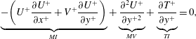 $$\begin{eqnarray}\displaystyle \underbrace{-\!\left(U^{+}\frac{\unicode[STIX]{x2202}U^{+}}{\unicode[STIX]{x2202}x^{+}}+V^{+}\frac{\unicode[STIX]{x2202}U^{+}}{\unicode[STIX]{x2202}y^{+}}\right)}_{MI}+\underbrace{\frac{\unicode[STIX]{x2202}^{2}U^{+}}{\unicode[STIX]{x2202}y^{+2}}}_{MV}+\underbrace{\frac{\unicode[STIX]{x2202}T^{+}}{\unicode[STIX]{x2202}y^{+}}}_{TI}=0, & & \displaystyle\end{eqnarray}$$
while for the channel
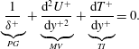 $$\begin{eqnarray}\displaystyle \underbrace{\frac{1}{\unicode[STIX]{x1D6FF}^{+}}}_{PG}+\underbrace{\frac{\text{d}^{2}U^{+}}{\text{d}y^{+2}}}_{MV}+\underbrace{\frac{\text{d}T^{+}}{\text{d}y^{+}}}_{TI}=0. & & \displaystyle\end{eqnarray}$$
Here
 $T^{+}\equiv -\overline{uv}^{+}$
represents the Reynolds stress. Note that in both cases the mean momentum balance is composed of three terms. From left to right the balance in the boundary layer includes mean inertia (MI), the mean viscous force (MV) and turbulent inertia (TI), whereas in the channel the mean pressure gradient (PG), the mean viscous force (MV) and turbulent inertia (TI) comprise the momentum balance.
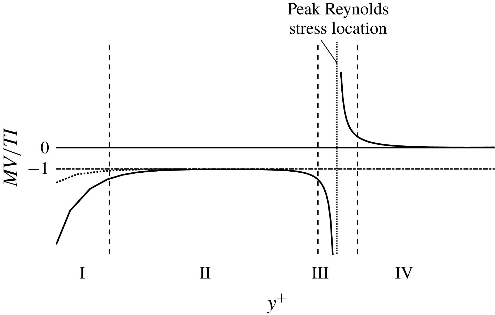
Unlike the balance of terms in the equations for laminar channel or boundary-layer flow, the terms in these equations are not of leading-order importance uniformly throughout the flow. In fact, the dominant balance (involving either two or three of the terms) changes with distance from the wall such that there is a well-defined four region structure (Wei et al.
Reference Wei, Fife, Klewicki and McMurtry2005), revealed through the ratio
 $MV/TI$
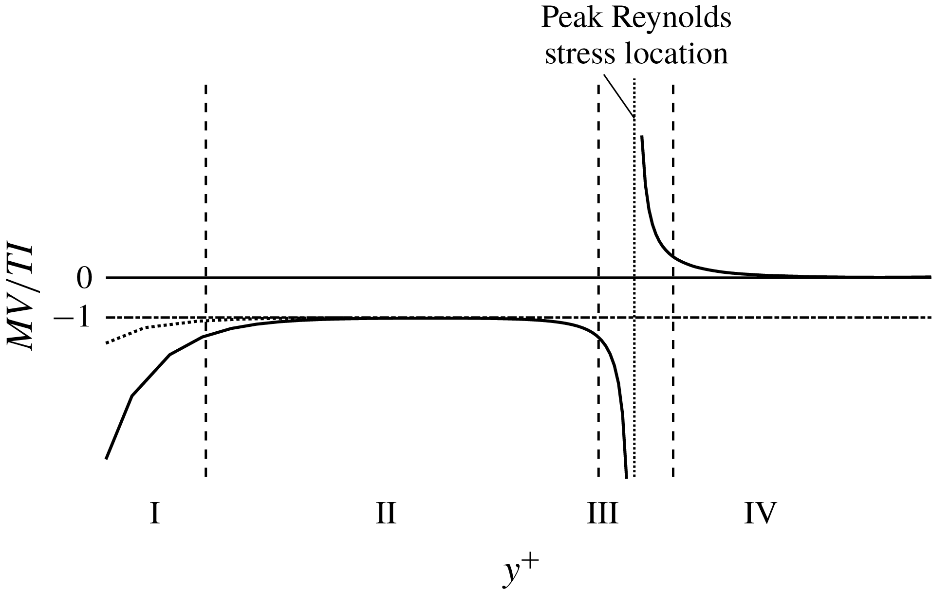
as shown in figure 1. Within three of these regions, (2.1) or (2.2) is brought into balance with two large terms dominating one small term (regions I, II and IV), while in another region (region III), all three terms contribute significantly to the balance. Thus, while all of the three terms in (2.1) or (2.2) are of leading order importance over some portion of the wall-normal domain
 $0\leqslant y\leqslant \unicode[STIX]{x1D6FF}$
, in three of the four regions there emerges only two dominant terms. An especially significant feature of this structure is that there exists a Reynolds number dependent position from the wall at which the mean viscous force becomes sub-dominant. This position is depicted by the outer edge of region III located at
 $y^{+}=2.6\sqrt{\unicode[STIX]{x1D6FF}^{+}}$
for channel flow. Beyond this location the mean momentum equation is inertially dominated, comprising a balance between the pressure gradient and turbulent inertia in the channel and between mean inertia and turbulent inertia in the boundary layer. The
 $\sqrt{\unicode[STIX]{x1D6FF}^{+}}$
dependence of this position is analytically predicted by the mean equation theory (Wei et al.
Reference Wei, Fife, Klewicki and McMurtry2005). The scaling properties of the region widths and their velocity increments for canonical turbulent channel flow are summarized in table 1.
Sketch of the four-region structure of turbulent wall-bounded flows at a representative, large Reynolds number: region I
 $|MI/PG|\simeq |MV|\gg |TI|$
; region II
 $|MV|\simeq |TI|\gg |MI/PG|$
; region III
 $|MI/PG|\simeq |MV|\simeq |TI|$
; region IV
 $|MI/PG|\simeq |TI|\gg |MV|$
(Wei et al.
Reference Wei, Fife, Klewicki and McMurtry2005).
Analysis of the mean momentum equation reveals an underlying similarity structure, one consequence of which is a logarithmic mean-velocity-profile solution determined by directly integrating the mean equation (Klewicki & Oberlack Reference Klewicki and Oberlack2015; Morrill-Winter et al.
Reference Morrill-Winter, Philip and Klewicki2017). This logarithmic profile arises as result of distance from the wall or
 $y$
-scaling, distinct from wall-flow representations that assume
 $y$
-scaling (e.g. Townsend’s attached-eddy framework, see Townsend (Reference Townsend1976), Perry & Marusic (Reference Perry and Marusic1995)). Here
 $y$
-scaling is analytically required for the mean momentum equation to admit an invariant form that respects the leading-order balance of terms with increasing
 $y$
. Specifically, the mean equation can be continuously rescaled into a single parameter-free form that is valid on each layer of a continuous and self-similar hierarchy of layers spanning a domain from
 $y=O(\unicode[STIX]{x1D708}/u_{\unicode[STIX]{x1D70F}})$
to
 $y=O(\unicode[STIX]{x1D6FF})$
. On each layer of this hierarchy, the rescaling is such that all of the terms in the mean equation are retained at leading order – a condition that reflects the changing average scale of the turbulent motions responsible for the wallward momentum flux with distance from the wall. The width
 $W$
of each hierarchy layer physically reflects the size of the turbulent motions responsible for wallward momentum transport (Klewicki et al.
Reference Klewicki, Philip, Marusic, Chauhan and Morrill-Winter2014), i.e. those motions associated with negative Reynolds stress. The theory prescribes a width and streamwise velocity increment for each layer: in the present model construction, a UMZ and its companion VF are effectively interpreted as one such layer on the layer hierarchy.
Magnitude ordering and scaling behaviours associated with the structure of the leading-order balance of mean forces in canonical turbulent channel flow. Note that PG, MV and TI refer to the mean pressure gradient, mean viscous force and turbulent inertia terms that, from left to right, are given in (2.2);
 $U_{c}$
is the mean centreline velocity; and
 $h$
is the channel half-height. Regions I, II, III and IV are indicated in figure 1.

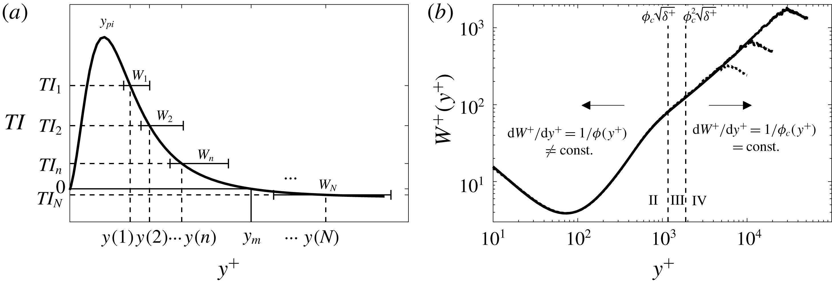
(a) Schematic depiction of the self-similar layer hierarchy admitted by the mean momentum equation.
 $TI$
 $=$
turbulent inertia. (b) Distribution of hierarchy layer widths
 $W^{+}(y^{+})$
as quantified using the channel flow DNS of Lee & Moser (Reference Lee and Moser2015). The line styles from top to bottom correspond to:
 $\unicode[STIX]{x1D6FF}^{+}=5200$
,
 $\unicode[STIX]{x1D6FF}^{+}=2000$
, and
 $\unicode[STIX]{x1D6FF}^{+}=1000$
. In the proposed model, each layer is associated with a UMZ and a VF.
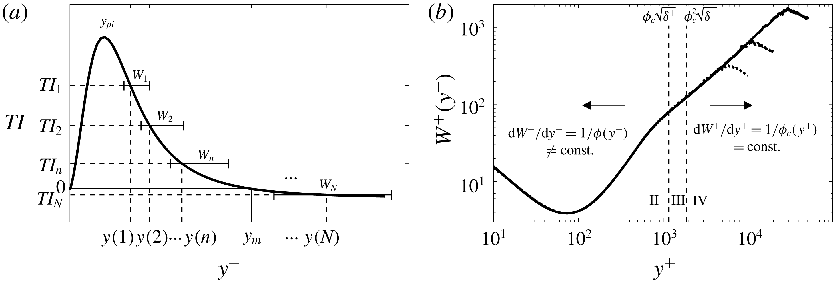
The sketch in figure 2(a) depicts that each point on the monotonically decreasing portion of the
 $\text{d}T^{+}/\text{d}y^{+}$
profile (i.e.
 $y>y_{pi}$
, where
 $y_{pi}$
denotes the peak location of the turbulent inertia) uniquely corresponds to a wall-normal position, and at each of these positions there resides a layer of finite width that is the member of the layer hierarchy at that point. Figure 2(b) plots these layer widths using DNS data. The layer hierarchy follows from the fact that at each distance from the wall, there is an average scale of motion at which the dynamics becomes inertially dominated (refer to region IV in table 1, in which the mean viscous forces are negligible). The theory predicts that, on average, the turbulent motions contributing to wallward momentum transport become inertially dominated at an increasing scale with increasing distance from the wall (Klewicki Reference Klewicki2013c
). The end result is that when
 $u_{\unicode[STIX]{x1D70F}}$
and the local layer width
 $W^{+}(y^{+})$
are used to normalize the mean equation under the requirement that all terms are of leading-order significance, then the re-normalized mean momentum equation becomes parameter free and invariant from one layer to the next. As can be seen in figure 2(b), wallward of the inertial domain the
 $W^{+}$
profile is a nonlinear function of
 $y^{+}$
, but invariant with
 $\unicode[STIX]{x1D6FF}^{+}$
. On the inertial domain, this invariance also holds (emerges) for increasing
 $\unicode[STIX]{x1D6FF}^{+}$
, but here
 $W^{+}$
is well-approximated by a linear function of
 $y^{+}$
, and increasingly so with increasing
 $\unicode[STIX]{x1D6FF}^{+}$
. Thus, while the layer hierarchy is self-similar both interior to and on the inertial domain, analyses on the inertial domain are simpler owing to the linear behaviour of
 $W^{+}(y^{+})$
.
The linearity of the
 $W^{+}$
profile on the inertial portion of the layer hierarchy underlies the logarithmic dependence on
 $y^{+}$
of the mean velocity profile. Here the mean momentum equation analysis predicts the emergence (with increasing
 $\unicode[STIX]{x1D6FF}^{+}$
) of an increasingly perfect dynamic self-similarity from one layer to the next. This self-similarity enables closure of the mean momentum equation, so that it can be directly integrated, yielding a similarity solution that takes the form of the universal logarithmic mean velocity profile as
 $\unicode[STIX]{x1D6FF}^{+}$
becomes large (Klewicki & Oberlack Reference Klewicki and Oberlack2015; Morrill-Winter et al.
Reference Morrill-Winter, Philip and Klewicki2017).
The absence of a leading-order mean viscous force on this logarithmic layer accords with the observed structure of UMZs and VFs. Namely, the viscous/vortical regions in the inertial domain occupy a diminishing fraction of the flow volume with increasing
 $\unicode[STIX]{x1D6FF}^{+}$
, as is physically reflected by the existence of the VFs. Conceptually, these motions effectively constitute ‘boundary layers’ within the turbulent boundary layer, a notion first promoted in Klewicki (Reference Klewicki2013a
) and explored in greater dynamical detail in Chini et al. (Reference Chini, Montemuro, White and Klewicki2017) and B. Montemuro (2018, private communication). A discrete (but valid) version of the hierarchy layer structure on the inertial domain provides a theoretically based recipe for assigning the wall-normal widths and velocity increments to the hierarchy layers with increasing distance from the wall, as described next.
Owing to their finite width, adjacent layers on the continuous hierarchy obviously overlap. By construction, however, the local scaling for any given layer formally holds over the extent of that layer. Thus, the most straightforward way to convert the continuous hierarchy description into a theoretically valid discrete representation is to stack adjacent layers such that the upper edge of one layer is the lower edge of the next. In fact, this construction already has been pursued by Klewicki et al. (Reference Klewicki, Philip, Marusic, Chauhan and Morrill-Winter2014), revealing a number of important features associated with the structure of the inertial domain. Among these is that the relative position of the start of one discrete hierarchy layer (
 $y_{i}^{+}$
) to the next (
 $y_{i+1}^{+}$
) on the inertial domain is given by
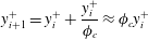 $$\begin{eqnarray}\displaystyle y_{i+1}^{+}=y_{i}^{+}+\frac{y_{i}^{+}}{\unicode[STIX]{x1D719}_{c}}\approx \unicode[STIX]{x1D719}_{c}y_{i}^{+} & & \displaystyle\end{eqnarray}$$
for non-negative integer
 $i$
, and the mean velocity increment from one layer to the next
 $$\begin{eqnarray}\displaystyle U_{i+1}^{+}-U_{i}^{+}\equiv \unicode[STIX]{x0394}U^{+}\approx \unicode[STIX]{x1D719}_{c}^{2}\ln \unicode[STIX]{x1D719}_{c}. & & \displaystyle\end{eqnarray}$$
In these expressions
 $\unicode[STIX]{x1D719}_{c}\approx (1+\sqrt{5})/2\approx 1.62$
is the so-called Fife similarity parameter, and is equal to the inverse of the asymptotically constant slope of the
 $W^{+}(y^{+})$
profile on the inertial domain (see figure 2
b). In the analysis,
 $\unicode[STIX]{x1D719}$
is the coordinate stretching function that produces an invariant form of the mean momentum equation on each hierarchy layer. This asymptotic constancy of
 $\unicode[STIX]{x1D719}$
(i.e.
 $\unicode[STIX]{x1D719}\rightarrow \unicode[STIX]{x1D719}_{c}$
) on the inertial domain also reflects a constant wall-normal flux of turbulent inertial force. Namely, under normalization by
 $W$
and
 $u_{\unicode[STIX]{x1D70F}}$
, the second derivative of the Reynolds stress approaches the constant value
 $2/\unicode[STIX]{x1D719}_{c}$
. A further mathematical consequence is that
 $\unicode[STIX]{x1D719}_{c}^{2}=1/\unicode[STIX]{x1D705}$
, where
 $\unicode[STIX]{x1D705}$
is the von Kármán constant.
The number of discrete layers
 $L$
on the inertial portion of the hierarchy increases logarithmically with
 $\unicode[STIX]{x1D6FF}^{+}$
, and thus under this discrete construction is countably infinite as
 $\unicode[STIX]{x1D6FF}^{+}\rightarrow \infty .$
The simplest way to generate an estimate for
 $L$
is to note that the inertial layer starts at
 $y^{+}\approx \unicode[STIX]{x1D719}_{c}^{2}\sqrt{\unicode[STIX]{x1D6FF}^{+}}$
(Klewicki et al.
Reference Klewicki, Philip, Marusic, Chauhan and Morrill-Winter2014) and that the hierarchy ends at
 $y^{+}\approx \unicode[STIX]{x1D6FF}^{+}/2$
(see figure 2
b), and that between these wall-normal locations the layers increase in scale according to the geometric progression given by (2.3). As an approximation, here we assume that this geometric progression extends all the way to
 $\unicode[STIX]{x1D6FF}$
and from this deduce that
 $$\begin{eqnarray}\displaystyle W_{max}^{+}\approx \unicode[STIX]{x1D6FF}^{+}=\unicode[STIX]{x1D719}_{c}^{L+2}\sqrt{\unicode[STIX]{x1D6FF}^{+}}. & & \displaystyle\end{eqnarray}$$
Subsequently solving for
 $L$
yields
 $L=\lfloor 1.04\,\text{ln}\,\unicode[STIX]{x1D6FF}^{+}-2\rfloor$
, where
 $\lfloor \bullet \rfloor$
is the floor function. A similar but somewhat more complicated estimation procedure yields an estimate for
 $L$
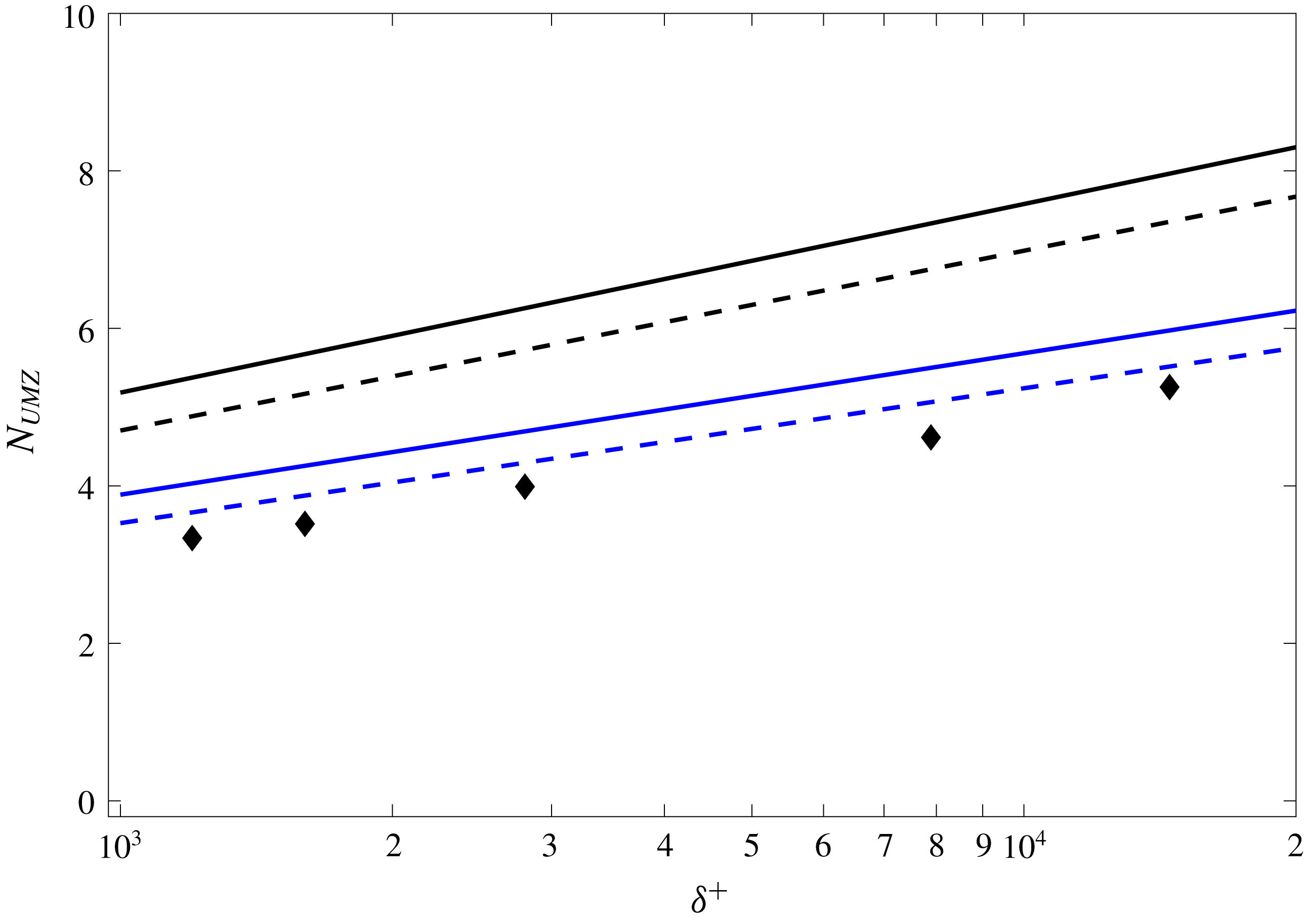
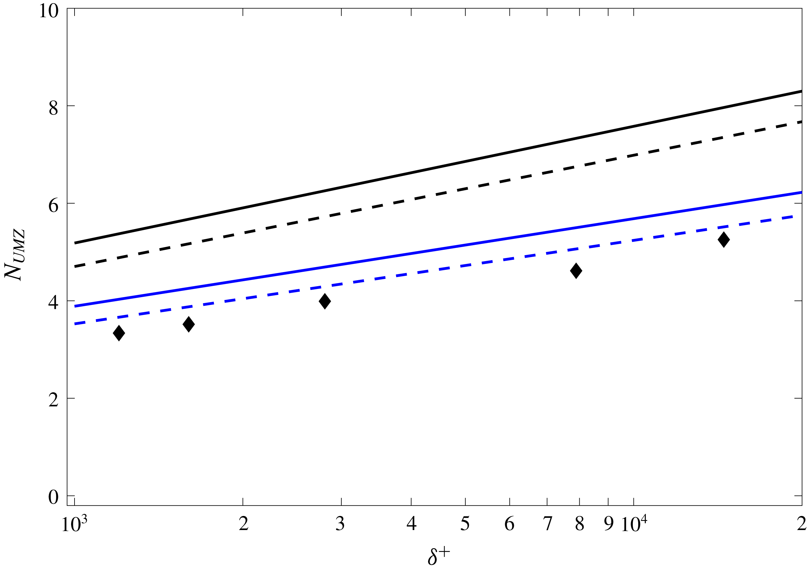
by accounting for the velocity increments associated with the VFs. As depicted in figure 3, these two estimates are nearly identical. Both, however, implicitly rely on the asymptotic approximation that all velocity variation occurs within the VFs and, similarly, that the VFs are negligibly thick relative to the UMZs. According to the present model construction (detailed below), the expectation is that
 $L$
roughly approximates the number of UMZs
 $N_{UMZ}$
in region IV of figure 1. These estimates and the recently reported measurements of
 $N_{UMZ}$
by de Silva et al. (Reference de Silva, Hutchins and Marusic2016) are plotted in figure 3. As is apparent, the asymptotic predictions consistently over-estimate the measured values. A number of sources, however, might contribute to the observed discrepancy. These include finite
 $\unicode[STIX]{x1D6FF}^{+}$
effects not accounted for in the analytical estimates, and the difficulties associated with accurately estimating
 $N_{UMZ}$
experimentally. Regarding the former, at finite
 $\unicode[STIX]{x1D6FF}^{+}$
not all of the velocity variation is contained in the VFs, and thus must be spread (in some unknown manner) throughout the UMZs (Klewicki Reference Klewicki2013a
). Unravelling precisely how this effect modifies the analytical estimates of
 $N_{UMZ}$
is not straightforward. Nevertheless, one can safely surmise that the effect reduces the estimate of
 $N_{UMZ}$
; for example, by considering the limiting case of smoothly distributed vorticity throughout region IV – a scenario with no discernible VFs. For laboratory-scale
 $\unicode[STIX]{x1D6FF}^{+}$
flows, Klewicki (Reference Klewicki2013a
) estimates that approximately 75 % of the mean velocity variation is contained within the VFs. Thus, a crude estimate for
 $N_{UMZ}$
at the
 $\unicode[STIX]{x1D6FF}^{+}$
of the measurements can be obtained simply by attenuating the asymptotic estimates according to the percentage of velocity variation contained in the VFs, i.e. by multiplying the asymptotic estimates by
 $0.75$
. As shown in figure 3, this ‘simple’ correction leads to a much better agreement with the data. Nevertheless, for the sake of simplicity, in the model construction described below we do not consider these effects, but instead invoke the asymptotic
 $\unicode[STIX]{x1D6FF}^{+}$
approximation by assigning all mean velocity variation to the VFs.
Number of uniform momentum zones
 $N_{UMZ}$
within region IV versus Reynolds number
 $\unicode[STIX]{x1D6FF}^{+}$
: ♦, as measured by de Silva et al. (Reference de Silva, Hutchins and Marusic2016); —— (upper black), as given by
 $L$
, where
 $L$
is the analytically estimated number of inertial hierarchy layers; - - - (upper black), as estimated by also accounting for the velocity increments. Lower lines (blue) ——, - - -, finite
 $\unicode[STIX]{x1D6FF}^{+}$
corrections to the asymptotic estimates by weighting the percentage of mean vorticity contained in the VFs.
3 Model construction
The detailed formulation of the UMZ/VF model is described in this section. The discussion is separated into two parts. First, the inertial-layer formulation, which enjoys the theoretical grounding given in § 2, is outlined. This is followed by an explication of the rationale for the model within the sub-inertial (i.e. near-wall) domain.
3.1 Inertial domain UMZ/VF model
The UMZ/VF structure on the inertial domain is represented by a set of
 $N$
discrete layers of concentrated vorticity (i.e. VFs) spaced according to (2.3). The velocity increment across each VF is given by (2.4). The following additional model prescriptions are made: the (wall-normal) fissure width
 $f_{w}^{+}=6$
(this choice is justified a posteriori in later sections); consistent with the theoretical framework, the lower boundary of the inertial domain is located at
 $y_{n_{VF}+1}^{+}=\unicode[STIX]{x1D719}_{c}^{2}\sqrt{\unicode[STIX]{x1D6FF}^{+}}$
, where
 $n_{VF}$
is the number of subinertial VFs; the mean velocity at this location is
 $U_{n_{VF}+1}^{+}=3.5+0.5U_{c}^{+}+1.26$
, which respectively accounts for the contributions from regions I–III; and the wall-normal position
 $y_{N_{VF}}^{+}$
and corresponding velocity
 $U_{N_{VF}}^{+}$
of the outer most fissure is obtained by setting the index
 $i=(N_{VF}-1)=L$
, where
 $N_{VF}$
is the number of VFs in the inertial region, in (2.3) and (2.4).
A modelling ambiguity arises for VFs of finite width, since the position of the (finite) VF is not uniquely prescribed by (2.3). In the absence of further dynamic or kinematic constraints, we empirically considered the respective ramifications associated with using the lower edge, the centroid and the upper edge as the reference position for any given VF at
 $y_{i}^{+}$
. Of these possibilities, only the centroid prescription avoids the asymmetries inherent in edge assignment, and leads to a computed mean profile that closely corresponds to the actual mean profile. The other choices either consistently under- or over-estimate the mean velocity. Concomitantly, associating
 $y_{i}^{+}$
with the centroid of the
 $i$
th VF also significantly improves the prediction of the higher statistical moment profiles.
The uniform velocity within each UMZ is associated with the edge velocities of the bounding VFs. In this regard, the lower (‘low’) and upper (‘up’) edge velocities of the
 $i$
th VF are defined as follows
 $$\begin{eqnarray}\displaystyle & \displaystyle U_{i,low}^{+}={\textstyle \frac{1}{2}}(U_{i}^{+}+U_{i-1}^{+}), & \displaystyle\end{eqnarray}$$
 $$\begin{eqnarray}\displaystyle & \displaystyle U_{i,up}^{+}={\textstyle \frac{1}{2}}(U_{i}^{+}+U_{i+1}^{+}). & \displaystyle\end{eqnarray}$$
Consequently, grid points comprising the lower UMZ, between the
 $y_{i-1}^{+}$
and
 $y_{i}^{+}$
centroids, have characteristic momentum
 $U_{i,low}^{+}$
and the grid points corresponding to the upper UMZ have characteristic momentum
 $U_{i,up}^{+}$
. Consistent with this set of rules, if there are
 $N$
VFs, then the number of UMZs is
 $N-1$
. Beyond the specification of a constant free-stream velocity boundary condition, the current model formulation does not account for a wake structure between the logarithmic region and free stream. For this reason, and because channel flow DNS currently attain larger
 $\unicode[STIX]{x1D6FF}^{+}$
than do boundary-layer DNS, we use the channel flow DNS data of Lee & Moser (Reference Lee and Moser2015) as a baseline for validating the model. This DNS was performed at
 $\unicode[STIX]{x1D6FF}^{+}\simeq 5200$
, with a centreline velocity
 $U_{c}^{+}\simeq 26.5$
. Using these parameter values, there are nominally six UMZs beyond the outer edge of region III, consistent with the asymptotic estimates given in figure 3.
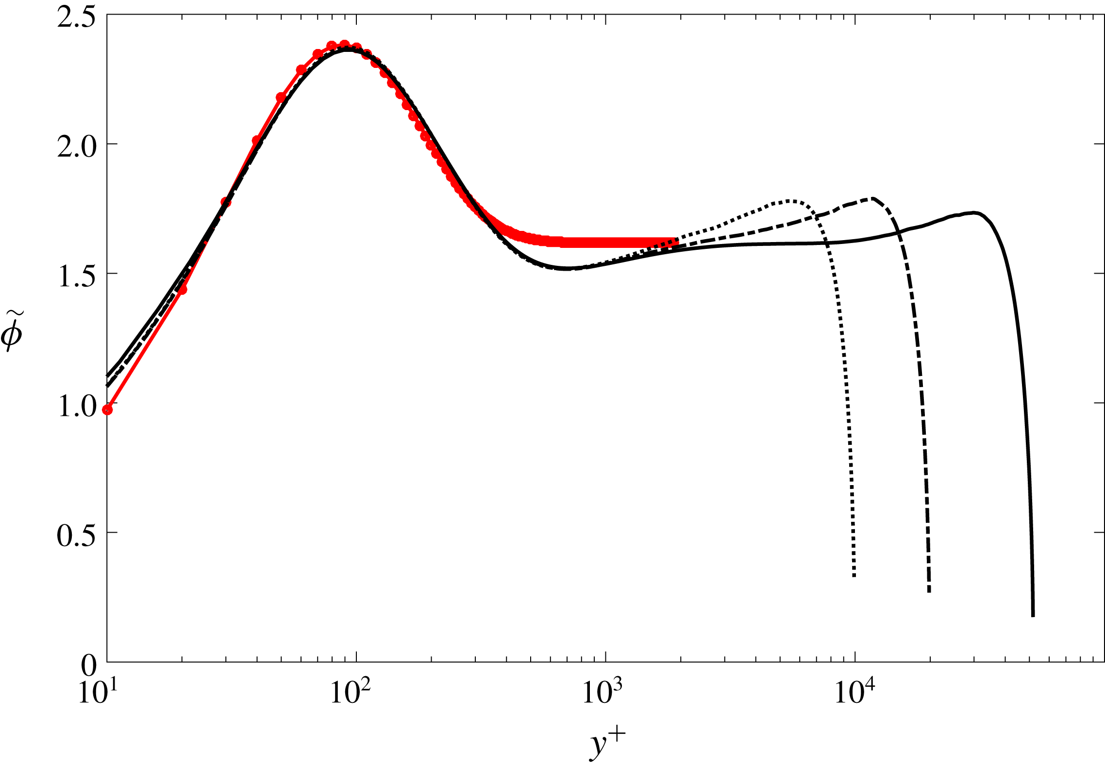
 $\tilde{\unicode[STIX]{x1D719}}(y^{+})$
versus
 $y^{+}$
computed for channel flow DNS of Lee & Moser (Reference Lee and Moser2015). The line styles correspond to: ——
 $\unicode[STIX]{x1D6FF}^{+}=5200$
, – - – - –
 $\unicode[STIX]{x1D6FF}^{+}=2000$
, - - - - - - -
 $\unicode[STIX]{x1D6FF}^{+}=1000$
,

 $\tilde{\unicode[STIX]{x1D719}}(y^{+})=-5.476\text{e}^{-0.218y^{+}}+4.203\text{e}^{-0.112y^{+}}+\unicode[STIX]{x1D719}_{c}$
.
3.2 Subinertial domain UMZ/VF model
The use of (2.3) and (2.4) to estimate the distribution of the vortical fissures and their characteristic velocities has a well-founded theoretical basis in an interior domain where the flow is inertially dominated, i.e.
 $\unicode[STIX]{x1D719}_{c}^{2}\sqrt{\unicode[STIX]{x1D6FF}^{+}}\lesssim y^{+}\lesssim \unicode[STIX]{x1D6FF}^{+}/2$
. As noted in the preceding subsection, we extend application of these formulas to the centreline, and therefore choose to compare with channel flow, since the deviation between the outer region mean velocity profile and the logarithmic profile tends to zero for channel flow as
 $\unicode[STIX]{x1D6FF}^{+}\rightarrow \infty$
. Closer to the wall, the mean momentum equation continues to admit a self-similar form, as evidenced by the universal
 $W^{+}$
profile in figure 2(b). The simple linear relationship between
 $y^{+}$
and
 $W^{+}$
is lost, however, and analytical representations have yet to be developed. This more complicated
 $W^{+}(y^{+})$
function coincides with a leading-order mean viscous force, an increasingly space-filling vorticity field as
 $y^{+}$
decreases, and an increasing significance of vorticity stretching and reorientation; e.g. see Klewicki (Reference Klewicki2013b
).
While more rigorously based treatment of the subinertial region must await analytical prediction of
 $W^{+}$
, herein we employ an empirical construction that meaningfully retains connection to a hierarchy of layers of increasing scale with increasing
 $y^{+}$
. To do this, we first note that within the region where
 $W^{+}\propto y^{+}$
(i.e. where
 $\unicode[STIX]{x1D719}=\unicode[STIX]{x1D719}_{c}$
) there is a well-defined asymptotic connection between the coordinate stretching function
 $\unicode[STIX]{x1D719}(y^{+})$
and the so-called indicator function. Namely,
 $$\begin{eqnarray}\displaystyle \unicode[STIX]{x1D719}^{2}(y^{+})\equiv \unicode[STIX]{x1D719}W^{+}\frac{\text{d}U^{+}}{\text{d}y^{+}}=y^{+}\frac{\text{d}U^{+}}{\text{d}y^{+}}. & & \displaystyle\end{eqnarray}$$
Here, it is useful to recall the analytical result that
 $\unicode[STIX]{x1D719}_{c}^{2}=1/\unicode[STIX]{x1D705}$
within the inertial sublayer (Klewicki Reference Klewicki2013c
). Although the equality between the two expressions for
 $\unicode[STIX]{x1D719}^{2}$
in (3.3) does not hold on the subinertial domain, the second expression provides a convenient surrogate (say,
 $\tilde{\unicode[STIX]{x1D719}}^{2}$
) for
 $\unicode[STIX]{x1D719}^{2}$
, since like
 $W^{+}$
these profiles do not vary with
 $\unicode[STIX]{x1D6FF}^{+}$
. Profiles of
 $\tilde{\unicode[STIX]{x1D719}}$
at different
 $\unicode[STIX]{x1D6FF}^{+}$
are plotted in figure 4. Thus, in the model implementation,
 $\tilde{\unicode[STIX]{x1D719}}(y^{+})$
is approximated by a nonlinear curve fit to the DNS data (also shown in figure 4). Use of this analytical fit then enables the allocation of spatial steps and their associated velocity increments (essentially VFs and UMZs) on the subinertial domain. Here, the velocity increments are found by rearranging and linearizing (3.3), which yields
 $$\begin{eqnarray}\displaystyle U_{i+1}^{+}=U_{i}^{+}+\tilde{\unicode[STIX]{x1D719}}(y_{i}^{+})^{2}\ln (y_{i+1}^{+}/y_{i}^{+}). & & \displaystyle\end{eqnarray}$$
Note that a logarithmic allocation of VFs, as chosen here, satisfies the linearization assumption, while preserving the notion of a scale hierarchy. Specifically, Sreenivasan & Bershadskii (Reference Sreenivasan and Bershadskii2006) provide compelling evidence that logarithmic expansions in
 $y$
provide an accurate means of representing the mean velocity and Reynolds stress profiles from
 $y=O(\unicode[STIX]{x1D708}/u_{\unicode[STIX]{x1D70F}})$
to
 $y=O(\unicode[STIX]{x1D6FF})$
by accounting for the number of hierarchical scales up to any given
 $y$
position.
3.3 Generating statistically independent ensembles
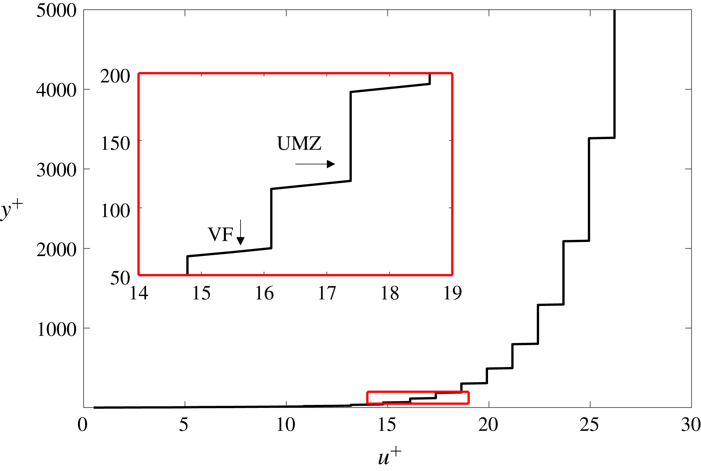
The master profile (see figure 5), which represents the most probable arrangement of the VFs, serves as the baseline from which the instantaneous velocity profiles are generated by repositioning the VFs in the boundary layer according to the following protocol
 $$\begin{eqnarray}\displaystyle y_{i,new}^{+}=y_{i}^{+}\pm {\mathcal{P}}[(y_{i}^{+}-y_{i-1}^{+})]. & & \displaystyle\end{eqnarray}$$
The statistical distribution
 ${\mathcal{P}}$
(Gaussian, uniform, exponential, beta, etc.) used to produce the new VF centroid position
 $y_{i,new}^{+}$
is empirically selected and a posteriori validated using the statistical moments computed from the instantaneous velocity profiles. The velocity is presumed to vary linearly across individual fissures. Note that, since each fissure is repositioned independently of its neighbours, multiple fissures are allowed to overlap in a given instantaneous profile; these overlaps are more likely to occur in the near-wall region. When fissures do overlap, the velocity across a fissure will vary piecewise linearly. Also note that, in the present model construction, the outer most VF is not allowed to move.
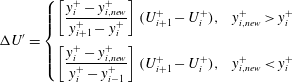
A critical finding of the a posteriori validation of the model is that satisfactory agreement with the DNS results cannot be obtained simply by repositioning the VFs. (This was found to be true regardless of the choice of model input parameters.) Specifically, compared to the DNS data, the magnitude of the modelled streamwise velocity variance is smaller across the entire channel and the sub-Gaussian behaviour of the velocity fluctuations within the inertial domain is not captured. To correct this deficiency, and informed by the analyses of Klewicki et al. (Reference Klewicki, Fife, Wei and McMurtry2007) and Eyink (Reference Eyink2008) showing that an outward flux of vorticity is connected with an inward flux of momentum (at least in the mean), a momentum-exchange mechanism is incorporated into the model. Specifically, when a vortical fissure is repositioned, its characteristic velocity at its new position is computed as follows
 $$\begin{eqnarray}\displaystyle U_{i,new}^{+}=U_{i}^{+}+\unicode[STIX]{x0394}U^{\prime }, & & \displaystyle\end{eqnarray}$$
where
 $$\begin{eqnarray}\displaystyle \unicode[STIX]{x0394}U^{\prime }=\left\{\begin{array}{@{}cc@{}}\displaystyle \left[\frac{y_{i}^{+}-y_{i,new}^{+}}{y_{i+1}^{+}-y_{i}^{+}}\right](U_{i+1}^{+}-U_{i}^{+}), & y_{i,new}^{+}>y_{i}^{+}\\ \displaystyle \left[\frac{y_{i}^{+}-y_{i,new}^{+}}{y_{i}^{+}-y_{i-1}^{+}}\right](U_{i+1}^{+}-U_{i}^{+}), & y_{i,new}^{+}<y_{i}^{+}\end{array}\right. & & \displaystyle\end{eqnarray}$$
is the momentum gain/loss as the VF moves to its new position (
 $y_{i,new}^{+}$
). Effectively, (3.6) reassigns the momentum distribution in the instantaneous profile compared to the master profile based on the wall-normal motion of a VF. Specifically, when a VF moves farther from the wall there is a momentum loss compared to the master profile. Conversely, as a VF moves toward the wall there is a momentum gain compared to the master profile. The magnitude of the momentum loss/gain by a VF is proportional to its relative wall-normal displacement compared to the master profile
 $[(y_{i}^{+}-y_{i,new}^{+})/(y_{i+1}^{+}-y_{i}^{+})]$
. The sensitivity of the modelled results to the momentum-exchange mechanism is explored in § 5.3.
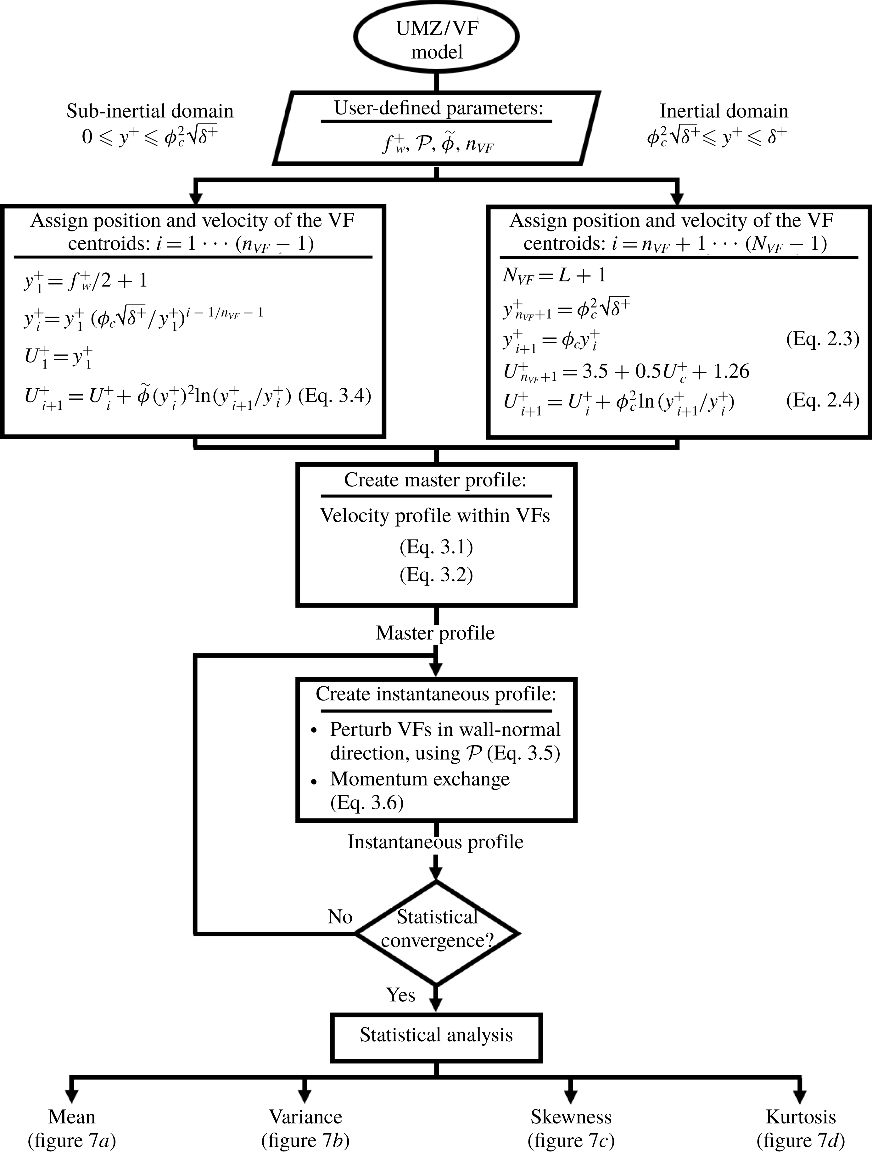
Flowchart of the UMZ/VF model construction. Note that
 $N_{VF}$
equals the greatest integer less than or equal to
 $1.04\,\text{ln}(\unicode[STIX]{x1D6FF}^{+})-1$
, i.e.
 $L+1$
, where
 $L$
roughly approximates the number of UMZs in region IV.
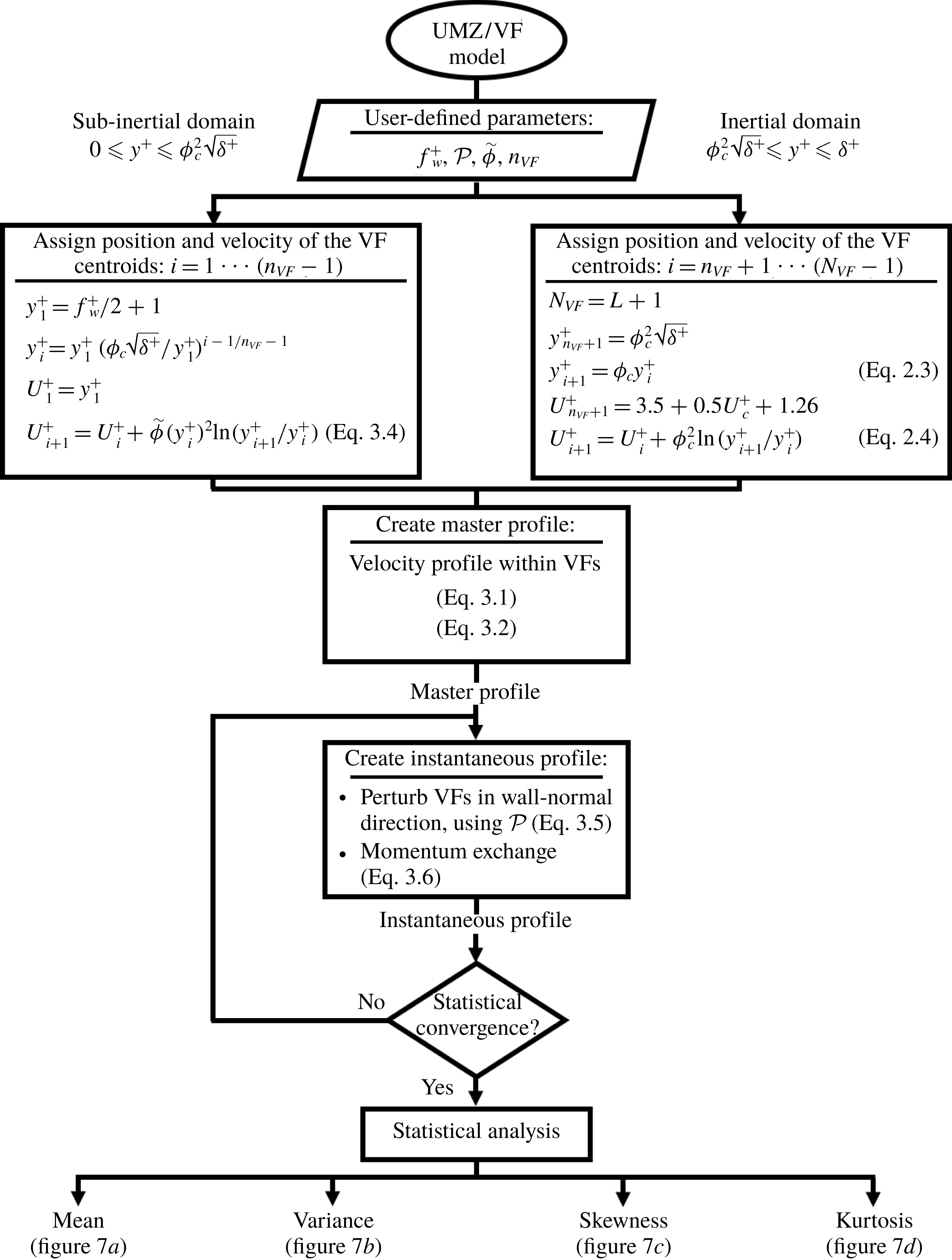
Figure 6 shows a flowchart of the UMZ/VF dynamical model. First, the flow is divided into two dynamically distinct domains: subinertial (
 $0\leqslant y^{+}\leqslant \unicode[STIX]{x1D719}_{c}^{2}\sqrt{\unicode[STIX]{x1D6FF}^{+}}$
) and inertial (
 $\unicode[STIX]{x1D719}_{c}^{2}\sqrt{\unicode[STIX]{x1D6FF}^{+}}\leqslant y^{+}\leqslant \unicode[STIX]{x1D6FF}^{+}$
). The fissure width
 $f_{w}^{+}$
is then selected as an empirical input to the model. Although
 $f_{w}^{+}\approx \sqrt{\unicode[STIX]{x1D6FF}^{+}}$
in the inertial domain, for ease of calculation and, particularly, for use in the subinertial domain, it is convenient to assign a much smaller fixed value. Nevertheless, we emphasize that (as shown in § 5.1) the modelled profiles are invariant for
 $f_{w}^{+}\lesssim \sqrt{\unicode[STIX]{x1D6FF}^{+}}$
in the inertial domain because VF widths are significantly smaller than the mean separation between adjacent VFs. Next, the number of VFs in each domain is determined (
 $n_{VF}$
and
 $N_{VF}$
for subinertial and inertial domains, respectively). For the inertial domain
 $N_{VF}=L+1$
while for the subinertial domain
 $n_{VF}$
is an empirical input to the model that is determined once
 $f_{w}^{+}$
and the positioning of the VFs are specified. In the inertial domain, the centroid of the first fissure is placed at
 $y_{n_{VF}+1}^{+}=\unicode[STIX]{x1D719}_{c}^{2}\sqrt{\unicode[STIX]{x1D6FF}^{+}}$
with characteristic velocity
 $U_{n_{VF}+1}^{+}=3.5+0.5U_{c}^{+}+1.26$
. The positioning and the characteristic velocity of the adjacent VFs are given by (2.3) and (2.4), respectively. In the subinertial domain, the position of the VF centroid closest to the wall is
 $y_{1}^{+}=(f_{w}^{+}+1)/2$
with characteristic velocity
 $U_{1}^{+}=y_{1}^{+}$
such that the lower edge of the first VF is at the wall and has zero velocity (i.e. in accord with the no-slip boundary condition). Adjacent VFs are logarithmically spaced moving outward from the wall. The characteristic velocities of the VFs in the subinertial domain are computed using the empirical relationship (3.4). Once the thickness, location and characteristic velocity of the VFs are specified, a master profile (see figure 5) that represents the most probable arrangement of VFs is developed using the UMZ construct given by (3.1) and (3.2). The VF positions are then perturbed in accord with (3.5), and new velocities are assigned to the VFs corresponding to their new wall-normal positions using the momentum-exchange formula (3.6). Note that, in a perturbed profile, subinertial and inertial VFs may cross, i.e. subinertial VFs can move into the inertial domain and conversely. This model therefore naturally embodies an inner-outer interaction consistent with the description of Klewicki et al. (Reference Klewicki, Fife, Wei and McMurtry2007) and the modulation studies of Mathis, Hutchins & Marusic (Reference Mathis, Hutchins and Marusic2009). Following this algorithm, a new instantaneous velocity profile associated with the perturbed UMZ/VF arrangement is generated. The process is repeated (e.g. 5000 times) to obtain sufficiently many independent realizations. Finally, the ensembles produced in this way are used to calculate statistical moment profiles of the streamwise velocity. It is worth noting that a typical run of 5000 realizations takes approximately one minute on a standard PC.
4 Turbulence statistics
As described in §§ 2 and 3, the UMZ/VF model is grounded in the analysis of the mean streamwise momentum equation at high Reynolds numbers but requires the specification of a modicum of empirically determined inputs. In particular, the results presented in this section have been produced using a positively skewed Gaussian distribution with a standard deviation
 $\unicode[STIX]{x1D70E}=1.6\unicode[STIX]{x0394}y_{i}^{+}$
, a fissure width
 $f_{w}^{+}=6$
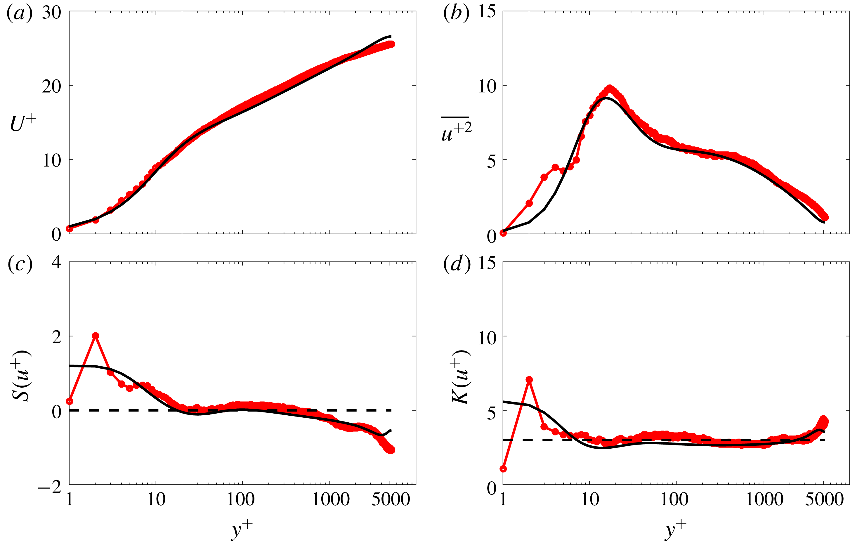
and a log-spaced distribution of the VF centroid positions in the subinertial domain. The VFs exchange momentum according to (3.6). The criteria used to select these parameters are examined in § 5, where a brief discussion of their physical meaning is also given. Figure 7 compares the mean
 $U^{+}$
, variance
 $\overline{u^{+2}}$
, skewness
 $S(u^{+})$
and kurtosis
 $K(u^{+})$
of the streamwise velocity
 $u$
generated from the UMZ/VF model with the corresponding statistics extracted from the channel flow DNS of Lee & Moser (Reference Lee and Moser2015). These results are discussed in detail below.
Statistical moments of the streamwise velocity computed using the UMZ/VF model (

 $\unicode[STIX]{x1D6FF}^{+}=5200$
(——). The horizontal dashed lines denote the value of the statistical moment for a Gaussian distribution.
4.1 Mean velocity
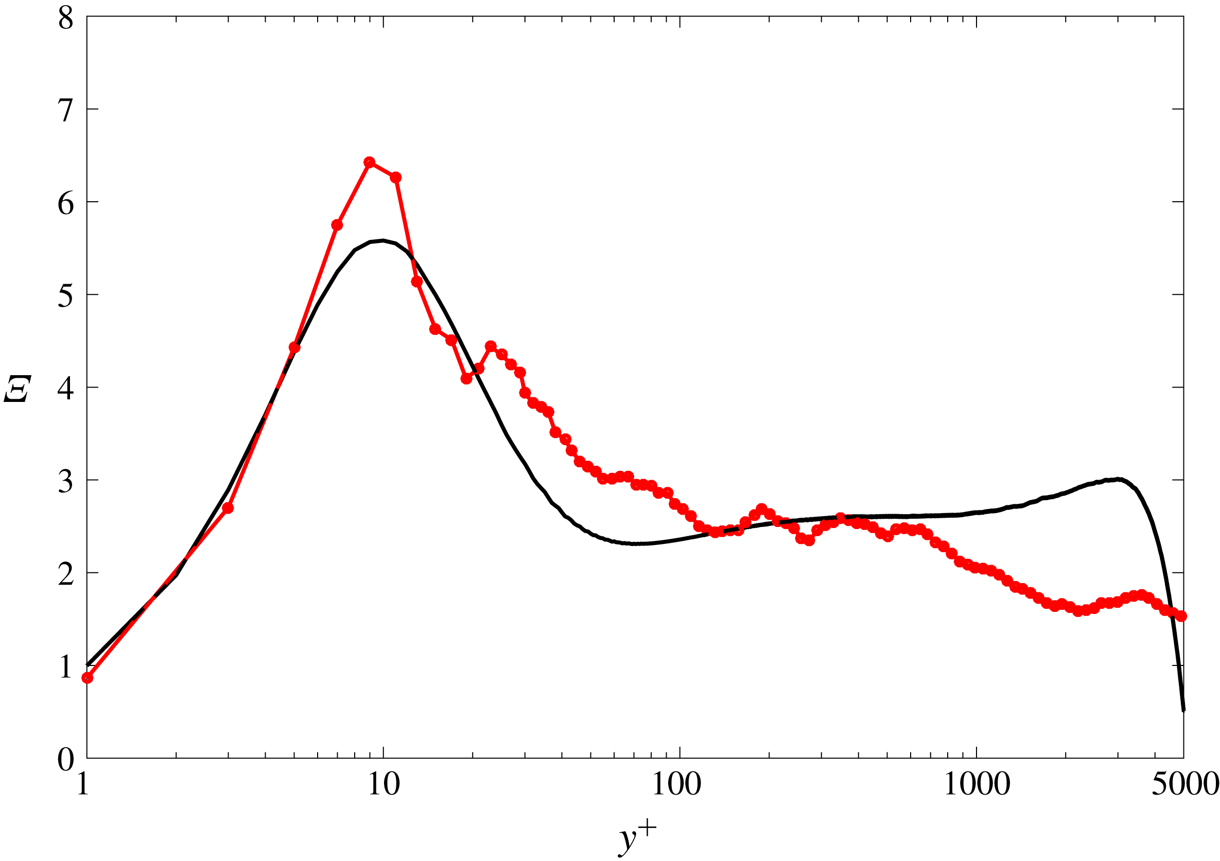
As shown in figure 7(a), the modelled mean velocity profile follows the DNS profile closely. The slight discrepancy between the modelled profile and the DNS data in the inertial domain is primarily attributable to a limitation of the model with respect to the wake region. More specifically, (i) the theoretical basis for the model, while only strictly valid on an interior portion of the inertial domain, is extended into and across the wake region; and (ii) the far-field boundary condition on the (instantaneous) streamwise velocity, intended to represent the ill-defined conditions at the edge of the boundary layer or at the centre of the channel, is imprecisely known. Regarding the latter issue, in the present construction of the model the outer VF is located at a fixed wall-normal position and ascribed a fixed characteristic velocity, given by (2.3) and (2.4), respectively. Unlike the other VFs, the outer VF is not allowed to move and exchange momentum. We have verified that when the outer VF is allowed to move, the modest deviation of the modelled mean velocity profile from the DNS data in the inertial domain is reduced; unfortunately, model results for the higher-order statistical profiles are negatively impacted. Despite the shortcomings of the model in the wake region, the so-called indicator function
 $\unicode[STIX]{x1D6EF}=y^{+}\text{d}U^{+}/\text{d}y^{+}$
computed from the model results nevertheless exhibits a pseudo-plateau region in an interior part of the inertial domain as evident in figure 8. This pseudo-plateau region indicates logarithmic
 $y$
-variation of the mean velocity profile in this region with a von Kármán constant
 $\unicode[STIX]{x1D705}=1/\unicode[STIX]{x1D6EF}\approx 0.4$
. Improvements to the model in the wake region will be one focus of future studies.
Importantly, the construction of the master profile is in itself not sufficient to guarantee good quantitative agreement between the modelled and DNS mean profiles. Additional factors do influence (albeit to a lesser extent) the ensemble-averaged modelled mean profile, namely: (i) the inner and outer boundary conditions (i.e. the location and velocity of the first and last fissure); (ii) the allowable wall-normal displacement of the VFs (which, if too small leads to spatial oscillations in the mean profile); and (iii) the reference position where the velocity is assigned for any given VF (e.g. lower edge, upper edge or centroid). Regarding the third factor, since the assigned velocity represents the mean velocity carried by a fissure, it must be placed at the centroid. If, instead, the assigned velocity is associated with the upper (lower) edge of the VF, the modelled mean profile lies above (below) the DNS profile.
The indicator function
 $\unicode[STIX]{x1D6EF}=y^{+}\text{d}U^{+}/\text{d}y^{+}$
computed from down-sampled mean velocity results from the UMZ/VF model (

 $\unicode[STIX]{x1D6FF}^{+}=5200$
(——).
4.2 Velocity variance
As evident in figure 7(b), the model is able to reproduce detailed features of the streamwise velocity variance. For instance, the inner peak location and amplitude, as well as the inflection point in the outer region, are accurately reproduced. Remarkably, another important characteristic quantitatively captured by the model is the apparent emergence of a plateau/second peak near the onset of the inertial domain,
 $y^{+}\approx 2.6\sqrt{\unicode[STIX]{x1D6FF}^{+}}$
. This position also delimits the start of a logarithmic decay of the variance, which extends to the end of the inertial domain (Marusic et al.
Reference Marusic, Monty, Hultmark and Smits2013). The model, however, fails to capture the variance very close to the wall (
 $y^{+}\lesssim 10$
). This discrepancy may be attributable to a number of factors; e.g. vortex stretching is not mechanistically represented in the model. (Note that the same explanation also presumably applies to the near-wall discrepancies in the skewness and kurtosis profiles; see below.)
4.3 Skewness of the velocity fluctuations
The skewness of the streamwise velocity fluctuations
 $S(u^{+})$
is shown in figure 7(c). As acknowledged above, the behaviour of the model in the near-wall region
 $y^{+}\lesssim 10$
requires further refinement, although reasonable agreement with the DNS skewness profile may be observed for
 $y^{+}\gtrsim 5$
. In this region, the model is able to reproduce the downward shift in the skewness, near
 $y^{+}\approx 30$
, in the vicinity of the sub-Gaussian peak. The sub-Gaussian trend in the DNS data is reproduced faithfully by the model out to
 $y\approx 0.8\unicode[STIX]{x1D6FF}^{+}$
, where the outer boundary condition then has a significant influence.
4.4 Kurtosis of the velocity fluctuations
The modelled streamwise velocity kurtosis
 $K(u^{+})$
profile is given in figure 7(d). The downward shift predicted by the UMZ/VF model occurs closer to the wall, i.e. near
 $y^{+}\approx 3$
, relative to the DNS data. As the profile crosses the Gaussian threshold
 $K(u^{+})=3$
, however, it consistently exhibits a sub-Gaussian behaviour across the whole domain, in accord with the DNS results. In contrast with the skewness profile, the modelled kurtosis exhibits good agreement with the DNS even out to the boundary-layer edge (
 $y^{+}=\unicode[STIX]{x1D6FF}^{+}$
).
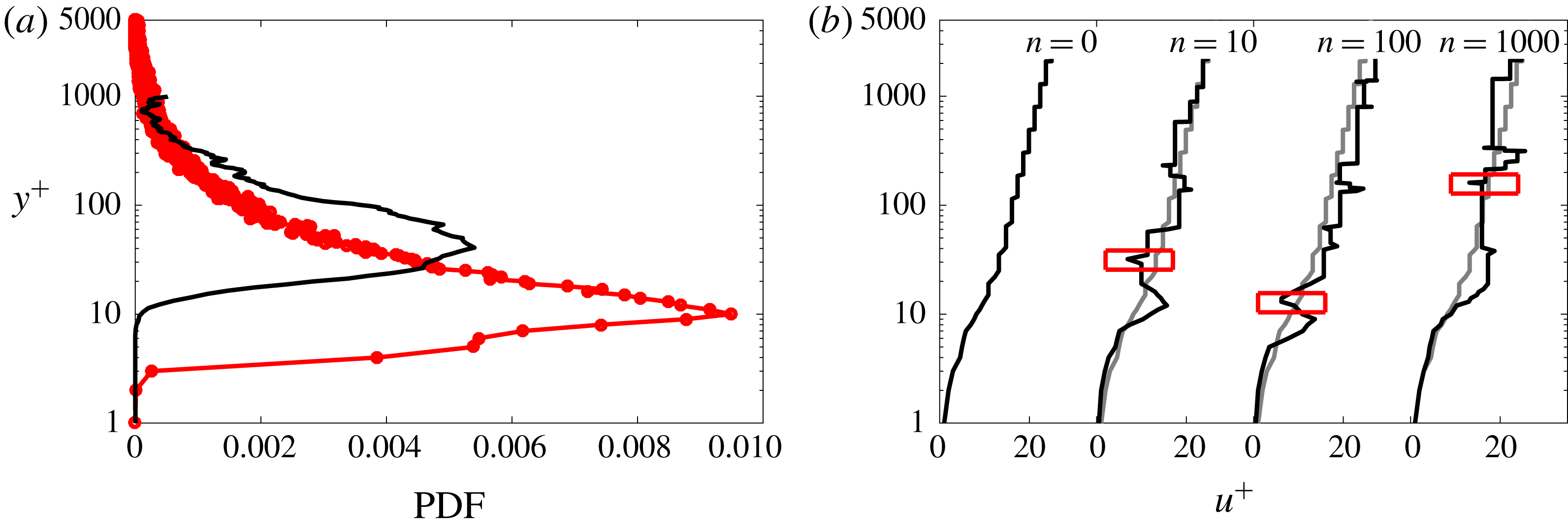
(a) The probability density function (PDF) of spanwise vorticity of opposite sign to that at the wall as computed from the model results (

 $\unicode[STIX]{x1D6FF}^{+}\simeq 1000$
(——) (Perlman et al.
Reference Perlman, Burns, Li and Meneveau2007; Li et al.
Reference Li, Perlman, Wan, Yang, Meneveau, Burns, Chen, Szalay and Eyink2008). (b) The master (
 $n=0$
) and three representative instantaneous velocity profiles (
 $n=10,100,1000$
). The red boxes in the instantaneous profiles highlight occurrences of strong positive instantaneous vorticity.
4.5 Probability density function of the positive spanwise vorticity
In addition to investigating the moments of the streamwise velocity, we also examined the modelled behaviour of the spanwise vorticity. Figure 9(a) shows the probability of occurrence of strong positive instantaneous vorticity (i.e. opposite in sign to that at the wall) throughout the boundary layer. The master (
 $n=0$
) and three representative instantaneous velocity profiles (
 $n=10,100,1000$
) are shown in figure 9(b). The red boxes in the instantaneous profiles highlight occurrences of strong positive instantaneous vorticity. The data in figure 7 were generated according to the following protocol. For each instantaneous velocity profile, the vorticity at the wall,
 $\unicode[STIX]{x1D714}(y=0)$
, is computed. Then the
 $y$
-positions in each of these instantaneous profiles where
 $\unicode[STIX]{x1D714}(y)\geqslant -0.1[\unicode[STIX]{x1D714}(y=0)]$
are detected and recorded. This procedure is repeated for all realizations. Next, at each
 $y$
-position across the channel domain, the number
 $N(y)$
of realizations for which
 $\unicode[STIX]{x1D714}(y)\geqslant -0.1[\unicode[STIX]{x1D714}(y=0)]$
is recorded. The probability of occurrence is computed as
 $N(y)/\!\int _{0}^{\unicode[STIX]{x1D6FF}^{+}}N(y)\,\text{d}y$
. As shown in Klewicki & Hill (Reference Klewicki and Hill1998), for example, there are frequent positive-vorticity events for
 $25\leqslant y^{+}\leqslant 35$
in the turbulent boundary layer, as can also be observed in turbulent channel flow data (see the solid black curve in figure 9(a) computed following the same protocol used for the modelled results). The model also predicts significant near-wall positive vorticity, albeit with a peak at
 $y^{+}\approx 10$
. This model discrepancy in the peak location of the probability density function (PDF) is conjectured to be attributable to neglecting vorticity stretching and reorientation, which drive inter-component transfers from
 $\tilde{\unicode[STIX]{x1D714}}_{z}$
to
 $\tilde{\unicode[STIX]{x1D714}}_{x}$
and
 $\tilde{\unicode[STIX]{x1D714}}_{y}$
.
Collectively, these comparisons indicate that the simple elements used to construct the UMZ/VF model are sufficient to quantitatively reproduce observed statistical behaviour over the interior of the boundary layer, although inaccuracies both very close to the wall and near the boundary-layer edge suggest that additional physical processes (e.g. near-wall vortex stretching) beyond those retained are significant in those regions. While feasible, refinements that incorporate such effects are not pursued here.
5 Sensitivity analysis
To assess the sensitivity of the model results to variations in the values of empirically chosen parameters, we next systematically adjust key model parameters within physically expected ranges and compare the resulting statistics to DNS data. Specifically, the impact of varying (i) the VF width, (ii) the probability distribution governing the VF displacements and (iii) the sign of the streamwise momentum exchange is investigated in sequence.
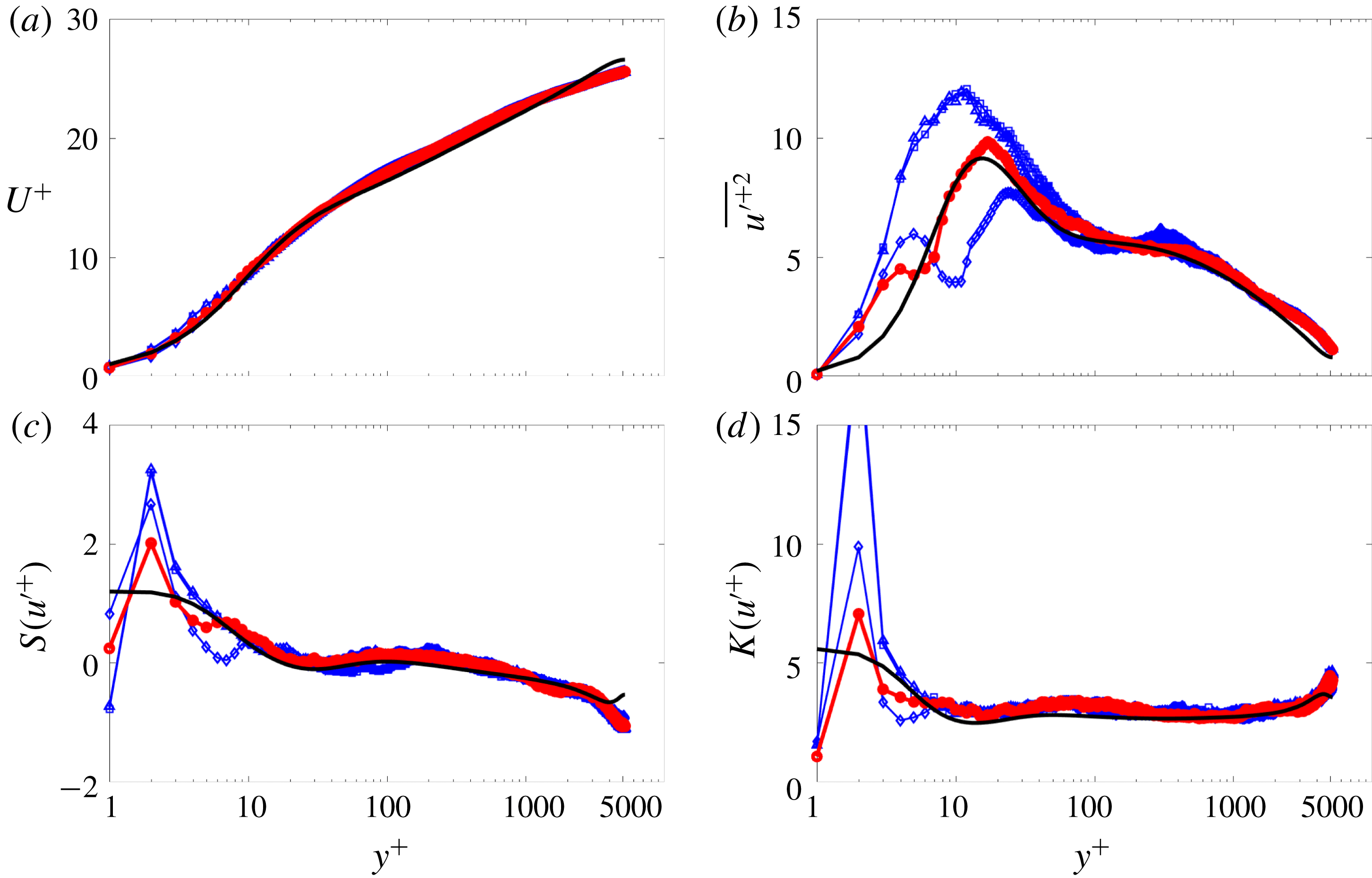
Statistical moments of the streamwise velocity field computed by the UMZ/VF model for various prescribed VF widths. The line styles correspond to:

 $f_{w}^{+}=6$
(best results),

 $f_{w}^{+}=2$
,

 $f_{w}^{+}=2{-}80$
,

 $f_{w}^{+}=10$
and —— DNS of Lee & Moser (Reference Lee and Moser2015) at
 $\unicode[STIX]{x1D6FF}^{+}=5200$
. The panels are the same as in figure 7.
5.1 VF width
The vortical fissure represents a region in the boundary layer across which the streamwise momentum jumps in magnitude from one UMZ to another. As discussed in § 1, Klewicki (Reference Klewicki2013b
) and Morrill-Winter & Klewicki (Reference Morrill-Winter and Klewicki2013) suggest that the inner-normalized thickness of a VF in the inertial domain is
 $O(\sqrt{\unicode[STIX]{x1D6FF}^{+}})$
, while, consistently, the measurements of Klewicki & Falco (Reference Klewicki and Falco1996), Chauhan, Philip & Marusic (Reference Chauhan, Philip and Marusic2014b
) and de Silva et al. (Reference de Silva, Philip, Hutchins and Marusic2017) suggest that
 $f_{w}$
is of the order of the Taylor microscale. Consequently, we investigated the behaviour of the model for various fixed, finite values of the VF width, e.g.
 $f_{w}^{+}=1,2,3,4,5,6\ldots ,$
as well as for a distribution of values across the boundary layer. Figure 10 shows four different cases: three different profiles for constant fissure widths
 $f_{w}^{+}=2,4$
and
 $6$
uniformly across the entire boundary layer, and a single profile for a variable fissure width modelled by a sigmoidal function with two horizontal asymptotes, i.e.
 $f_{w}^{+}=2$
at the wall and
 $f_{w}^{+}=80$
in the inertial domain, respectively. As anticipated, the statistical comparisons confirm that the model is independent of
 $f_{w}$
in the inertial region, where the VF width is significantly smaller than the width of the adjacent UMZs. On the other hand, precise specification of the VF width clearly has a significant impact in the vicinity of the wall (
 $y^{+}\lesssim 30$
), where the model results exhibit larger variation and larger discrepancies with the DNS data. The latter observation is likely attributable to the intense velocity gradients present in the near-wall region, and the absence of vortex stretching in the model. In contrast, we have modelled the velocity jump across each fissure with a simplistic linear relationship (§ 3.1).
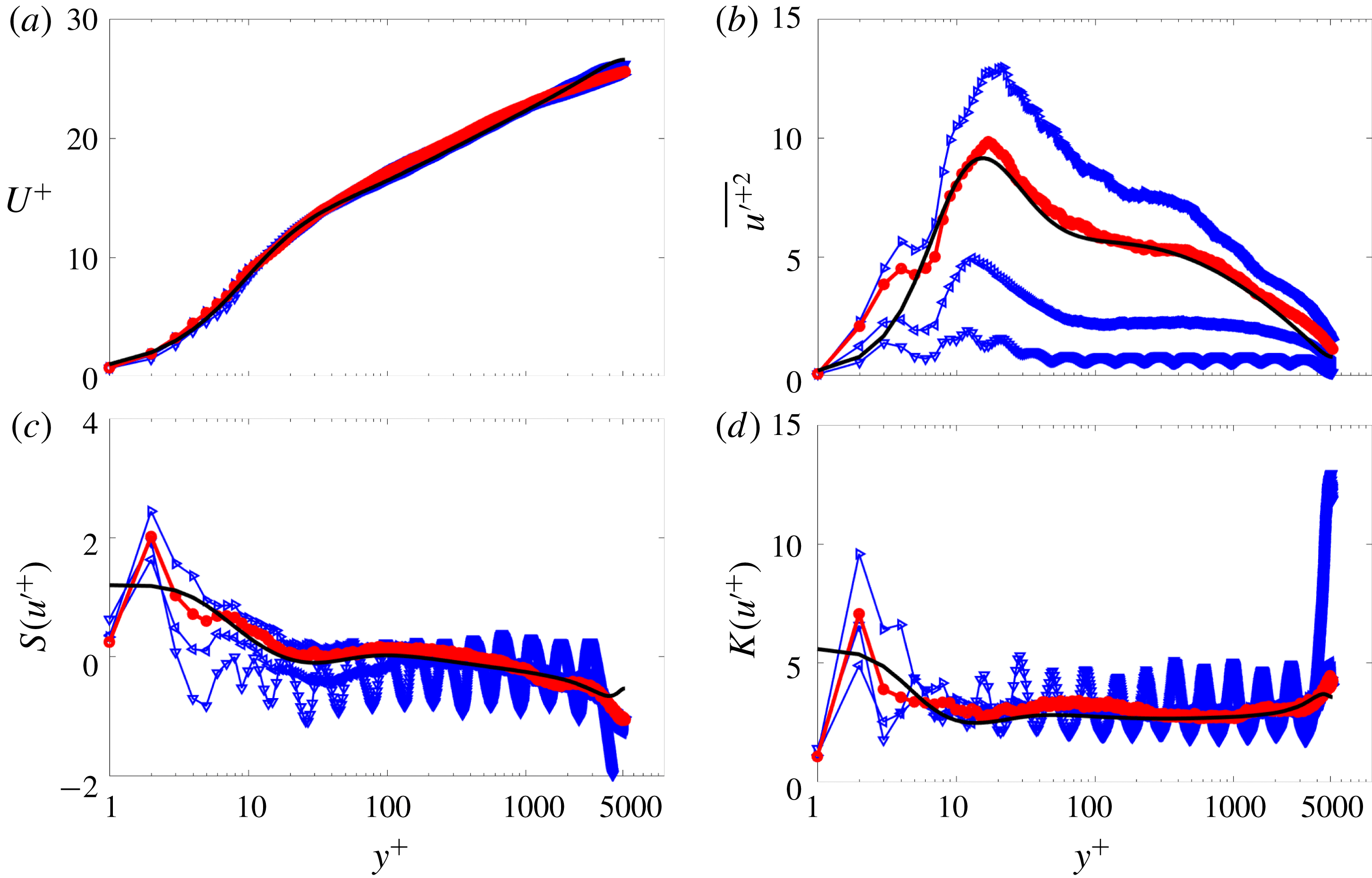
Statistical moments of the streamwise velocity field computed using the UMZ/VF model with a positively skewed Gaussian distribution of wall-normal VF displacements for various, specified standard deviations. The line styles correspond to:

 $\unicode[STIX]{x1D70E}=1.6\unicode[STIX]{x0394}y_{i}$
(best results),

 $\unicode[STIX]{x1D70E}=0.5\unicode[STIX]{x0394}y_{i}$
,

 $\unicode[STIX]{x1D70E}=1.0\unicode[STIX]{x0394}y_{i}$
,

 $\unicode[STIX]{x1D70E}=2.0\unicode[STIX]{x0394}y_{i}$
, and —— DNS of Lee & Moser (Reference Lee and Moser2015) at
 $\unicode[STIX]{x1D6FF}^{+}=5200$
. The panels are the same as in figure 7.
5.2 Wall-normal motion
The wall-normal motion of the VF centroids is dictated by the probability distribution
 ${\mathcal{P}}$
in (3.5). Since the statistical distribution associated with these motions is not known, a judicious mix of empiricism and physical reasoning must be employed to select a suitable surrogate. Several PDFs were explored but, for brevity, we present only the most pertinent results. In short, by optimizing the model we found that the best agreement with the channel and boundary-layer data were obtained for PDFs derived from the normal distribution family. In this regard, Eisma et al. (Reference Eisma, Westerweel, Ooms and Elsinga2015) and de Silva et al. (Reference de Silva, Hutchins and Marusic2016, Reference de Silva, Philip, Hutchins and Marusic2017) recently have reported experimental evidence of the fluctuations in the wall-normal positions of the edges of the UMZs (here associated with the VF centroids). Crucially, they postulate that the PDF of these motions exhibits a near-Gaussian distribution with a positive skewness in the near-wall region.
Figure 11 presents results for a skewed Gaussian distribution for a range of standard deviations
 $\unicode[STIX]{x1D70E}$
. A key result is that the VFs must displace, on average, at least
 $\unicode[STIX]{x1D70E}=\unicode[STIX]{x0394}y_{i}^{+}$
units from their original position in order to ensure smooth mean profiles and a comparably uniform distribution of UMZs, as is necessary to recover the high–low–high UMZ-intermittency structure in the instantaneous streamwise velocity profile (de Silva et al.
Reference de Silva, Hutchins and Marusic2016). Conversely, it is observed that an excessive wall-normal displacement causes the model to over-predict the higher-order statistical profiles. The results plotted in figure 11 reveal that the variance is more sensitive than
 $S(u^{+})$
or
 $K(u^{+})$
to variations in the range of allowable wall-normal displacements. Inspection of this figure suggests that
 $\unicode[STIX]{x1D70E}=1.6\unicode[STIX]{x0394}y_{i}^{+}$
provides the most reasonable agreement with the DNS data. Although not reproduced here, examination of the residual values between the modelled and DNS profiles quantitatively confirms this observation.
5.3 Streamwise momentum-exchange mechanism
Statistical moments of the streamwise velocity field computed using the UMZ/VF model with three different momentum-exchange mechanisms. The line styles correspond to:


 $\unicode[STIX]{x1D6FF}^{+}=5200$
is shown by ——. The panels are the same as in figure 7.
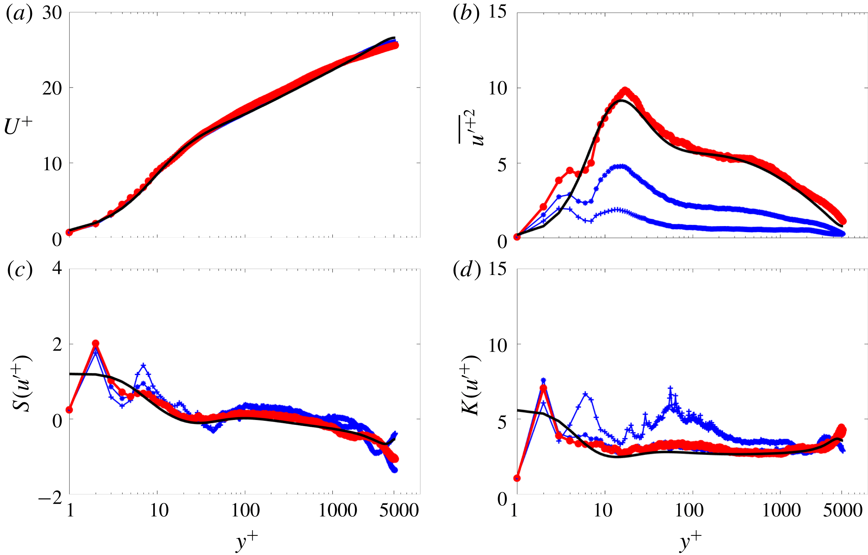
The statistics for three different VF momentum-exchange scenarios are shown in figure 12. The three scenarios are (i) the momentum exchange is computed using (3.6) in which VFs gain (lose) momentum as they move toward (away from) the wall; (ii) the VFs lose (gain) momentum as they move toward (away from) the wall by reversing the sign of the right-hand side of (3.6); and (iii) the momentum exchange is suppressed. Inspection of figure 12 shows that the first scenario (i.e. positive exchange momentum) clearly exhibits the best agreement with the DNS data. It is also worth noting that, as for the other sensitivities, the mean velocity is the statistical profile that is least sensitive to variations in the model parameters. In contrast, to reproduce the higher-order statistics in turbulent flows, a more detailed representation of the VF dynamics is necessary.
6 Conclusion
A simple dynamical model of the UMZ/VF structure of the instantaneous streamwise velocity in turbulent boundary layers has been constructed and validated via comparison with DNS channel flow data for a boundary-layer equivalent
 $\unicode[STIX]{x1D6FF}^{+}\approx 5200$
. The formulation of the model involves separate treatment of two primary domains based upon the characteristic four-region structure derived from analysis of the mean momentum equation: the inertial domain, where the mean and turbulent inertia are dominant; and the subinertial domain, where the mean viscous force is of leading-order importance. The velocity and length scaling employed within the inertial region of the model is a discrete representation analytically developed from the continuous hierarchy-layer width distribution associated with formally constructing an invariant (self-similar) form of the mean momentum equation. This analytical scaling has been shown to be consistent with experimental characterization of the UMZ/VF structure (see §§ 2 and 3). For the subinertial domain, a surrogate length and velocity scaling is explored. Here, we exploit the self-similar and universal behaviour of the coordinate stretching function
 $\unicode[STIX]{x1D719}$
in the near-wall region (see figure 4) by using an empirical curve fit of this function
 $\tilde{\unicode[STIX]{x1D719}}$
to predict the subinertial streamwise velocity according to (3.4). Given that the length scale analysis does not show the same behaviour as its inertial counterpart, a logarithmic distribution of VFs in the subinertial region is used. This prescription retains consistency with the number of hierarchical layers increasing logarithmically with
 $y$
. The concatenation of these two domains completes the specification of the UMZ/VF master streamwise velocity profile over the entire boundary layer. This master profile is used in conjunction with a minimal protocol for randomly displacing the VFs to generate realizations of the instantaneous streamwise velocity, from which various statistics of the streamwise velocity and spanwise vorticity are computed.
Our study reveals that the most compelling results are obtained by using a positively skewed Gaussian distribution with a standard deviation
 $\unicode[STIX]{x1D70E}=1.6\unicode[STIX]{x0394}y^{+}$
, a fissure width
 $f_{w}^{+}=6$
, and a momentum-exchange mechanism that is consistent with the known inverse fluxes of momentum (inward) and vorticity (outward) relative to the wall. The selection criteria for these parameters are thoroughly discussed in § 5. Here, we remark that although reproduction of key aspects of the statistical properties of turbulent boundary layers also has been achieved using certain other structure-based models that utilize different flow structures (e.g. Perry & Chong Reference Perry and Chong1982, Perry & Marusic Reference Perry and Marusic1995, Adrian Reference Adrian2007) these models rely to varying degrees on a priori knowledge of the eddy structure geometry. In contrast, the present model contains two elements, UMZs and VFs, that empirically are known to become distinct as
 $\unicode[STIX]{x1D6FF}^{+}\rightarrow \infty$
. Herein we demonstrate that this model, once properly tuned, can reproduce the main characteristics of the first four moments of the streamwise velocity. We also note that once tuned, the results at different
 $\unicode[STIX]{x1D6FF}^{+}$
acquired using identical model parameters (not shown) suggest that ‘ideal tuning’ of the model will produce only a weak Reynolds number dependence. Furthermore, to our knowledge, the UMZ/VF model developed here is the only structure-based model that robustly captures the sub-Gaussian behaviour of the velocity fluctuations in the inertial domain.
The results in figure 12 indicate that the modelled even higher-order moments, in particular, are sensitive to the momentum-exchange mechanism. This feature of the model allows the VFs to gain or lose momentum as they are displaced toward or away from the wall, respectively. We postulate that this mechanism is consistent with the mean similarity structure of turbulent wall-flow dynamics as described by Klewicki (Reference Klewicki2013b ). Specifically, for turbulent channel flow the turbulent shear stress gradient can be expressed by
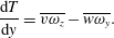 $$\begin{eqnarray}\displaystyle \frac{\text{d}T}{\text{d}y}=\overline{v\unicode[STIX]{x1D714}_{z}}-\overline{w\unicode[STIX]{x1D714}_{y}}. & & \displaystyle\end{eqnarray}$$
Since the model presented here incorporates the wall-normal repositioning of VFs, the only operative net momentum transport mechanism is associated with the
 $\overline{v\unicode[STIX]{x1D714}_{z}}$
term (i.e.
 $\overline{w\unicode[STIX]{x1D714}_{y}}=0$
). This feature is somewhat similar to Taylor’s vorticity transport theory (Taylor Reference Taylor1932). The first term in (6.1) thus dictates the vorticity dynamics across the boundary layer, e.g. if
 $\overline{v\unicode[STIX]{x1D714}_{z}}<0$
, it is associated with the advection of momentum toward the wall (a mean momentum sink), while if
 $\overline{v\unicode[STIX]{x1D714}_{z}}>0$
, it is associated with the advection of momentum away from the wall (a mean momentum source). This dynamics also is supported by the recent experimental evidence of C. Bautista (2018, private communication), where quadrant analysis of the
 $v\unicode[STIX]{x1D714}_{z}$
product revealed that the
 $Q4(-v,\unicode[STIX]{x1D714}_{z})$
events are dominant across the entire extent of the boundary layer for a wide range of
 $\unicode[STIX]{x1D6FF}^{+}$
. In the context of the mean vorticity dynamics, these events are associated with the advection of high momentum fluid toward the wall. On the other hand, the vorticity stretching mechanism associated with the
 $\overline{w\unicode[STIX]{x1D714}_{y}}$
term, important in the sub-inertial domain, is not included in the model. Therefore, we speculate that if this mechanism were to be incorporated into the UMZ/VF model framework, the results in the near-wall region could be improved considerably. Nevertheless, the agreement between the DNS and modelled streamwise velocity moments lends credence to the conceptual notion that the turbulent boundary layer comprises logarithmically many viscous (if not laminar) internal layers. If this conceptual picture is valid, then a crucial question is: what three-dimensional dynamical processes nonlinearly sustain the staircase-like structure of the streamwise velocity in turbulent wall flows? We are attempting to address this fundamental issue in companion work (Chini et al.
Reference Chini, Montemuro, White and Klewicki2017; B. Montemuro, 2018, private communication).
Acknowledgements
This study was supported by National Science Foundation Award no. 1437851 and partially supported by the Australian Research Council. The authors are thankful to C.M. de Silva et al. (The University of Melbourne), R. Moser (University of Illinois), J. Kim (University of California, Los Angeles) and Y. Li et al. (Johns Hopkins Turbulence Database) for providing access to their data.