1 Introduction
Mixing of reactive scalars is an interesting generalization of passive scalar mixing. In reactive mixing, high-concentration regions spread not only because of diffusion and advection, but also because of local reactive growth – the total quantity of scalar need not be conserved. Such spreading can be nonlinear and complex, making prediction challenging. However, reliable prediction would have practical implications for a wide range of systems, including wildfires (Hargrove et al. Reference Hargrove, Gardner, Turner, Romme and Despain2000; Punckt et al. Reference Punckt, Bodega, Kaira and Rotermund2015), combustion (Coriton, Frank & Gomez Reference Coriton, Frank and Gomez2016), industrial mixing (Nienow, Edwards & Harnby Reference Nienow, Edwards and Harnby1997; Kresta et al. Reference Kresta, Atiemo-Obeng, Paul and Atiemo-Obeng2004), pharmaceutical manufacture (Gendrin, Roggo & Collet Reference Gendrin, Roggo and Collet2008; Schlick et al. Reference Schlick, Umbanhowar, Ottino and Lueptow2014) and phytoplankton bloom dynamics (Martin Reference Martin2003). In each system, the local motion of reaction fronts, which separate reacted from unreacted regions, provides a simplified representation and provides insight into common dynamics. Local measurement of reaction front motion can uncover features that do not appear when only the spatially averaged front speed is considered, as in many prior studies (Xin Reference Xin2000; Abel et al. Reference Abel, Celani, Vergni and Vulpiani2001; Kiselev & Ryzhik Reference Kiselev and Ryzhik2001; van Saarloos Reference van Saarloos2003). Local understanding is the first step toward prediction and control, with goals like maximizing or minimizing spreading.
In this paper, we will investigate the growth of a reactive scalar advected in quasi-two-dimensional (quasi-2-D) flow, common in reactive mixing experiments. Although three-dimensional (3-D) reactive mixing experiments have recently been undertaken (Doan et al. Reference Doan, Simons, Lilienthal, Solomon and Mitchell2018), quasi-2-D systems simplify experiment, instrumentation and analysis while capturing rich dynamics, including optimal flow properties (Nevins & Kelley Reference Nevins and Kelley2016), mixing barriers (Gowen & Solomon Reference Gowen and Solomon2015) and sensitivity to boundary conditions (Beauvier, Bodea & Pocheau Reference Beauvier, Bodea and Pocheau2017). Two-dimensional data are sometimes gathered by averaging over one spatial dimension (Coriton, Frank & Gomez Reference Coriton, Frank and Gomez2013), and more often gathered by driving reactive mixing in a thin layer (Gowen & Solomon Reference Gowen and Solomon2015; Nevins & Kelley Reference Nevins and Kelley2016; Beauvier et al. Reference Beauvier, Bodea and Pocheau2017; Chevalier, Salin & Talon Reference Chevalier, Salin and Talon2017; Wang et al. Reference Wang, Tithof, Nevins, Colón and Kelley2017). However, even thin-layer fluid experiments have at least some three-dimensionality; their flows and reaction fields depend on depth, and that dependence often goes unmeasured. As we will show, unmeasured 3-D processes, especially shear, can cause surprising results. We will also suggest methods for minimizing the effects of shear and three-dimensionality.
The growth of a scalar concentration field (such as a chemical reaction product)
 $C(\boldsymbol{x},t)$
depends on advection (flow), reaction and diffusion. (Here
 $\boldsymbol{x}=x\hat{\boldsymbol{x}}+y\hat{\boldsymbol{y}}+z\hat{\boldsymbol{z}}$
is position and
 $t$
is time.)
 $C$
is typically normalized to range from 0 (unreacted) to 1 (reacted), and in experiments, is often approximated by measuring the local colour of the reacting solution (Wood & Ross Reference Wood and Ross1985). If we consider the case where the local reaction rate depends only on existing concentration, and diffusion is independent of concentration, then the field
 $C$
obeys the advection–reaction–diffusion (ARD) equation
 $$\begin{eqnarray}\displaystyle \frac{\unicode[STIX]{x2202}C}{\unicode[STIX]{x2202}t}+\boldsymbol{u}\boldsymbol{\cdot }\unicode[STIX]{x1D735}C=D\unicode[STIX]{x1D6FB}^{2}C+\unicode[STIX]{x1D6FC}F(C), & & \displaystyle\end{eqnarray}$$
where
 $\boldsymbol{u}$
is the velocity of the fluid in which the scalar is reacting,
 $D$
is the diffusion coefficient,
 $\unicode[STIX]{x1D6FC}$
is a reaction rate coefficient and
 $F(C)$
is a dimensionless reaction term. Chemical reactions that involve multiple species are modelled by systems of ARD equations, one for each chemical species
 $C_{i}\;(i\in \{1,N\})$
with its own reaction term
 $F_{i}(C_{1},C_{2},\ldots ,C_{n})$
. Here, however, we will focus on the simple case of a single reaction product. The flow
 $\boldsymbol{u}$
obeys the Navier–Stokes equation, which we presume is independent of
 $C$
, so that it need not be solved simultaneously with equation (1.1).
Although equation (1.1) rigorously governs the behaviour of a reactive scalar field, simplifying the equation can lead to new intuition about reaction dynamics. In particular, reaction fronts, which are surfaces that separate unreacted from reacted regions, have proved conceptually useful. For many reactions,
 $F(C=0)=F(C=1)=0$
, and
 $F(C)>0$
for
 $0<C<1$
, such that regions of moderate concentration quickly react and become nearly saturated (
 $C\approx 1$
). Typically,
 $C\approx 0$
or
 $C\approx 1$
over much of the domain. In that case, equation (1.1) shows that
 $\unicode[STIX]{x2202}C/\unicode[STIX]{x2202}t\approx 0$
except in the small regions where
 $\unicode[STIX]{x1D735}C$
is large, since the advection and diffusion terms in equation (1.1) both involve spatial variation. Thus the fronts that separate
 $C\approx 0$
regions from
 $C\approx 1$
regions locate the essential dynamics of the system, and front propagation is a natural descriptor of system evolution. Analogous reasoning holds for excitable chemical systems in which
 $F(C)>0$
only in the smaller range
 $C_{0}<C<1$
(where
 $C_{0}$
is a dimensionless excitation threshold).
To understand the velocity of any differential element of a reaction front, first consider what the motion must be in stagnant and uniform flows. The total velocity,
 $\boldsymbol{w}$
, must move outward at the chemical speed
 $v$
in stagnant. Then in uniform flow the exact solution is obtained by simply adding the flow velocity. The eikonal equation for ARD systems is then created by assuming this simple summation works for non-uniform flows as well (Spangler & Edwards Reference Spangler and Edwards2003)
 $$\begin{eqnarray}\displaystyle \boldsymbol{w}=\boldsymbol{u}+v\hat{\boldsymbol{n}}. & & \displaystyle\end{eqnarray}$$
Here
 $\hat{\boldsymbol{n}}$
is the local unit normal to the front. By definition,
 $\hat{\boldsymbol{n}}$
points in the direction of decreasing
 $c$
(opposite
 $\unicode[STIX]{x1D735}c$
). This equation is much simpler than equation (1.1) to understand and implement numerically, and therefore it is a powerful tool for predicting ARD systems.
The motion of reaction fronts, and the eikonal approximation for describing that motion, were used to great effect in the development of the theory of burning invariant manifolds (BIMs) (Mahoney et al.
Reference Mahoney, Bargteil, Kingsbury, Mitchell and Solomon2012, Reference Mahoney, Li, Boyer, Solomon and Mitchell2015). Burning invariant manifolds are dynamical barriers to front propagation, located where
 $\boldsymbol{u}\boldsymbol{\cdot }\hat{\boldsymbol{m}}=-v$
, with
 $\hat{\boldsymbol{m}}$
being the unit vector locally normal to the BIM. The
 $\hat{\boldsymbol{m}}$
direction of the BIM causes these to be one-sided barriers. There, the flow velocity is fast enough in the direction opposite to the front propagation, such that
 $\boldsymbol{w}$
is strictly tangent to the BIM according to equation (1.2). Thus BIMs attract fronts and predict where fronts can propagate and where they cannot. Seeing the power of fronts for capturing the dynamics of reactive mixing, we recently developed an automated algorithm for measuring the instantaneous, local chemical velocity
 $v\hat{\boldsymbol{n}}$
and the instantaneous, local total front speed
 $\boldsymbol{w}$
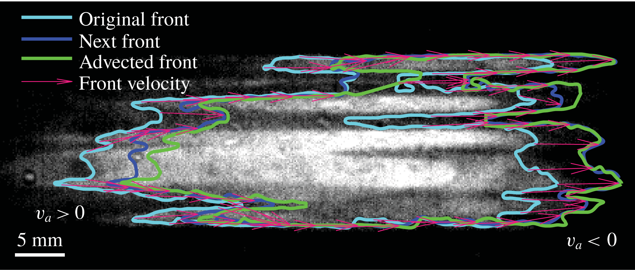
(Nevins & Kelley Reference Nevins and Kelley2017, Reference Nevins and Kelley2018). Figure 1 demonstrates the front tracking technique. The algorithm is written for 2-D simulations or quasi-2-D experiments and works by identifying reaction fronts, advecting them forward according to the known flow
 $\boldsymbol{u}$
and measuring the perpendicular displacement between the advected front and the front observed at a later time.
Experimental measurements of chemical reaction fronts using front tracking. A thin layer of reacting fluid is imaged from above, appearing bright where product concentration is high and dark where product concentration is low. By definition, reaction fronts are located at the edges of regions that are brighter than a user-defined threshold. To measure the local front speed, a front (Original Front) is advected numerically using the known flow velocity field and compared to a front at a later time (Next Front). The perpendicular distance that separates them is attributed to the chemical velocity
 $v_{a}\hat{\boldsymbol{n}}$
, and the total velocity
 $\boldsymbol{w}$
is calculated using equation (1.2). In this example, the fluid flows from left to right, but the next front is outside the advected front at left (
 $v_{a}>0$
), and inside it at right (
 $v_{a}<0$
).

The front tracking algorithm, like BIM theory, is built on equation (1.2), but without the simplifying assumption that the chemical speed is a constant
 $v=v_{0}$
. The constant front speed assumption has been broadly applied, despite neglecting higher-order effects like curvature, Ekman pumping and shear. Curvature is known to affect chemical speed according to
 $v=v_{0}+D\unicode[STIX]{x1D705}$
, where
 $\unicode[STIX]{x1D705}$
is the curvature (Keener Reference Keener1986). The effect has been observed in experiments having length scales of the order of microns (Foerster, Muller & Hess Reference Foerster, Muller and Hess1988) but is generally negligible in aqueous experiments at larger length scales because
 $D\sim 10^{-3}~\text{mm}^{2}~\text{s}^{-1}$
. A notable exception to this is pinning of fronts to obstacles (Chevalier et al.
Reference Chevalier, Salin and Talon2017). The BIM theory (using the
 $v=v_{0}$
assumption) agrees closely with experimental measurements in a variety of flows with a variety of parameters (Gowen & Solomon Reference Gowen and Solomon2015; Megson et al.
Reference Megson, Najarian, Lilienthal and Solomon2015; Doan et al.
Reference Doan, Simons, Lilienthal, Solomon and Mitchell2018). Other studies have predicted (Xin Reference Xin2000; Abel et al.
Reference Abel, Celani, Vergni and Vulpiani2001; Kiselev & Ryzhik Reference Kiselev and Ryzhik2001; van Saarloos Reference van Saarloos2003) or observed (Mehrvarzi & Paul Reference Mehrvarzi and Paul2014; Beauvier et al.
Reference Beauvier, Bodea and Pocheau2017) variation in the total velocity
 $\boldsymbol{w}$
or the space-averaged chemical speed, while confirming that the local chemical speed
 $v$
is essentially constant.
However, in recent quasi-2-D experiments, we observed (Nevins & Kelley Reference Nevins and Kelley2018) chemical speeds far in excess of
 $v_{0}$
, apparently contradicting the
 $v=v_{0}$
assumption. The effect was much larger than could be explained by curvature (Foerster et al.
Reference Foerster, Muller and Hess1988) or Ekman pumping, which could happen within the vortex cells without global rotation (Solomon & Mezić Reference Solomon and Mezić2003). We performed the experiments in a thin, horizontal layer of reacting solution and measured flow velocity
 $\boldsymbol{u}$
, but were able to measure only its horizontal components, and only at the top of the layer. Therefore, vertical flow was a potential source of complications, although we were careful not to drive flows fast enough to cause the onset of substantial vertical motions (Kelley & Ouellette Reference Kelley and Ouellette2011; Tithof, Martell & Kelley Reference Tithof, Martell and Kelley2018). Moreover, we observed apparently high chemical speeds even in directions misaligned with electric field (Feeney, Schmidt & Ortoleva Reference Feeney, Schmidt and Ortoleva1981; Sevčiková & Marek Reference Sevčiková and Marek1983). These puzzling observations could be due to either a physical mechanism not included in equation (1.2), or a complication associated with doing experiments in reactive mixing.
In this paper we focus on the second possibility: an experimental complication. We will show that vertical shear can change both the magnitude and sign of the apparent chemical speed
 $v_{a}$
in front tracking experiments, depending on the orientation of the front relative to the flow, such that
 $v_{a}\neq v$
. We will compare experimental measurements of
 $v_{a}$
to simulations that assume the true chemical speed is
 $v_{0}$
but account for front deformation by vertical shear. Close agreement between simulation and experiment will show that vertical shear explains nearly all of the apparent deviation from
 $v_{0}$
. Vertical shear is caused by the no-slip boundary condition at the base of the thin layer and smears reaction fronts in a way that makes measuring the local concentration
 $C$
more complicated. In most experiments, concentration is accessed optically, by measuring the depth-averaged concentration, but shear changes the vertical concentration profile. Many prior and future quasi-2-D reactive mixing experiments are subject to similar shear effects, so shear must be considered when interpreting results. The effect persists even if
 $\boldsymbol{u}\boldsymbol{\cdot }\hat{\boldsymbol{z}}=0$
everywhere (where
 $\hat{\boldsymbol{z}}$
points upward). Shear originating from a no-slip boundary condition has been shown to have a major effect before, especially in the case of Poiseuille flow (Edwards Reference Edwards2002; Leconte et al.
Reference Leconte, Martin, Rakotomalala and Salin2003). We will further show that vertical shear can be substantially reduced, allowing reactive mixing experiments that are more nearly two-dimensional, if the reacting layer is separated from the no-slip boundary below it by a lubrication layer.
In § 2 we describe the results of simulating front propagation throughout the depth of a single thin layer, and extract the chemical speeds that would be measured in an experiment using optical methods. In § 4 we repeat the discussion, but consider a two-layer system in which the thin, reacting layer is bounded below by an immiscible, dielectric, lubrication layer to reduce shear. In § 3 we repeat the discussion, but consider a single-layer system in which both boundaries are subject to no-slip conditions and flow is driven by a pressure difference (the Hele-Shaw configuration). In § 5 we describe the experimental apparatus and methods we developed to test the predictions of §§ 2 and 4. In § 6 we present the results of single- and two-layer experiments, showing good agreement with our simulations, including a significant reduction in apparent deviation from
 $v=v_{0}$
in the two-layer system. The paper closes with a summary and outlook in § 7.
2 Simulations of single-layer system
We begin our investigation by simulating reactive mixing in a single, thin layer of fluid, with flow driven horizontally, a common configuration for quasi-2-D experiments (Gowen & Solomon Reference Gowen and Solomon2015; Nevins & Kelley Reference Nevins and Kelley2016, Reference Nevins and Kelley2017, Reference Nevins and Kelley2018; Wang et al.
Reference Wang, Tithof, Nevins, Colón and Kelley2017; Chevalier et al.
Reference Chevalier, Salin and Talon2017; Beauvier et al.
Reference Beauvier, Bodea and Pocheau2017). The layer is subject to a no-slip boundary condition at the solid floor that supports it and a no-penetration condition at its top surface. (We will consider no-slip conditions on both boundaries in § 3.) In the laboratory, it is convenient to study chemical reactions whose products have a different colour than the reactants, so that concentration
 $C$
can be measured optically. Common candidates include the Belousov–Zhabotinsky reaction (Zaikin & Zhabotinsky Reference Zaikin and Zhabotinsky1970; Wood & Ross Reference Wood and Ross1985; Esptein Reference Esptein1987; Scott Reference Scott1994), the iodate arsenous acid reaction (Atis et al.
Reference Atis, Saha, Auradou, Salin and Talon2013; Chevalier et al.
Reference Chevalier, Salin and Talon2017) and acid-base reactions (Arratia & Gollub Reference Arratia and Gollub2006). In thin-layer experiments, the local colour depends on the average concentration across the reacting layer, and reaction fronts can be defined as the locations where the brightness crosses some user-defined threshold. For simple forms of the reaction term
 $F(C)$
, equation (1.1) can be solved analytically in the one-dimensional case and predicts concentration profiles that maintain their shape while propagating, so that front speed measurements are insensitive to the choice of threshold. If the concentration is uniform across the layer depth, fronts located this way are unambiguous, and three-dimensionality need not be considered. However, if the concentration varies with depth, more care is required. The sensitivity of concentration measurements to variation with depth contrasts with other measurements. For example, tracer particles used for measuring the flow
 $\boldsymbol{u}$
can be selected with a density that causes them to float atop the reacting layer. Their motion samples only the top of the layer, without depth averaging, so 3-D effects are negligible until upwellings and downwellings become substantial (Kelley & Ouellette Reference Kelley and Ouellette2011; Tithof et al.
Reference Tithof, Martell and Kelley2018). When locating reaction fronts, however, three-dimensionality must be considered more carefully. We begin with a simple simulation.
2.1 Velocity profile
In this section, we describe simulations to explore the implications of vertical shear for reactive mixing experiments. To simplify the problem, we consider a steady, planar flow that is uniform at the free surface of the layer:
 $\boldsymbol{u}(x,y,z=h)=U\hat{\boldsymbol{x}}$
. Here
 $h$
is the layer thickness, and we choose
 $z=0$
at the bottom of the layer. The flow must vary with depth, but we will assume that the forcing is such that we can separate the planar motion from its
 $z$
dependence (Dolzhanskii, Krymov & Manin Reference Dolzhanskii, Krymov and Manin1992; Figueroa et al.
Reference Figueroa, Demiaux, Cuevas and Ramos2009; Suri et al.
Reference Suri, Tithof, Mitchell, Grigoriev and Schatz2014). We expect this construction to provide a reasonable approximation for the non-uniform flows as well, because a similar approach by Suri et al. (Reference Suri, Tithof, Mitchell, Grigoriev and Schatz2014) closely matched experiments with non-uniform flows. Considering uniform flow also gives us clear expectations for front velocity, since uniform flow differs from the well-studied
 $\boldsymbol{u}=0$
case only by a Galilean transformation.
Such a flow can be generated by applying a vertical magnetic field
 $\boldsymbol{B}=B(z)\hat{\boldsymbol{z}}$
and passing a uniform, horizontal electrical current with density
 $\boldsymbol{J}=J\hat{\boldsymbol{y}}$
through the reacting layer. Including the resulting Lorentz force, the Navier–Stokes equation that governs the flow is
 $$\begin{eqnarray}\displaystyle \frac{\unicode[STIX]{x2202}\boldsymbol{u}}{\unicode[STIX]{x2202}t}+\boldsymbol{u}\boldsymbol{\cdot }\unicode[STIX]{x1D735}\boldsymbol{u}=-\frac{1}{\unicode[STIX]{x1D70C}}\unicode[STIX]{x1D735}P+\frac{\unicode[STIX]{x1D707}}{\unicode[STIX]{x1D70C}}\unicode[STIX]{x1D6FB}^{2}\boldsymbol{u}+\frac{JB}{\unicode[STIX]{x1D70C}}\hat{\boldsymbol{x}}-g\hat{\boldsymbol{z}}, & & \displaystyle\end{eqnarray}$$
where
 $\unicode[STIX]{x1D70C}$
is the density of the fluid,
 $P$
is the pressure,
 $\unicode[STIX]{x1D707}$
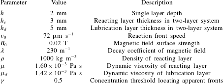
is the dynamic viscosity and
 $g$
is the gravitational acceleration. We consider a magnetic field that varies vertically, as it does in experiments (Figueroa et al.
Reference Figueroa, Demiaux, Cuevas and Ramos2009) with magnets arranged below the reacting layer,
 $$\begin{eqnarray}\displaystyle B(z)=B_{0}e^{-\unicode[STIX]{x1D706}z}. & & \displaystyle\end{eqnarray}$$
Here
 $B_{0}$
and
 $\unicode[STIX]{x1D706}$
are empirical constants measured for our apparatus and listed in table 1. To satisfy
 $\unicode[STIX]{x1D735}\boldsymbol{\cdot }\boldsymbol{B}=0$
, the magnetic field must also have a horizontal component that varies with
 $z$
, but the vertical force it produces is negligible compared to gravity, so we will not discuss it further. The flow occurs in a layer of infinite extent in
 $x$
and
 $y$
. At
 $z=0$
, we impose a no-slip boundary condition
 $\boldsymbol{u}=0$
. At
 $z=h$
, we impose a no-penetration boundary condition
 $\boldsymbol{u}\boldsymbol{\cdot }\hat{\boldsymbol{z}}=0$
and require that the shear be zero:
 $\unicode[STIX]{x2202}u_{x}/\unicode[STIX]{x2202}z=0$
. Solving equation (2.1), we find
 $$\begin{eqnarray}\displaystyle \boldsymbol{u}=u_{x}\hat{\boldsymbol{x}}=\frac{JB_{0}}{\unicode[STIX]{x1D707}\unicode[STIX]{x1D706}}\left(\frac{1}{\unicode[STIX]{x1D706}}-\frac{e^{-\unicode[STIX]{x1D706}z}}{\unicode[STIX]{x1D706}}-e^{-h\unicode[STIX]{x1D706}}z\right)\hat{\boldsymbol{x}}. & & \displaystyle\end{eqnarray}$$
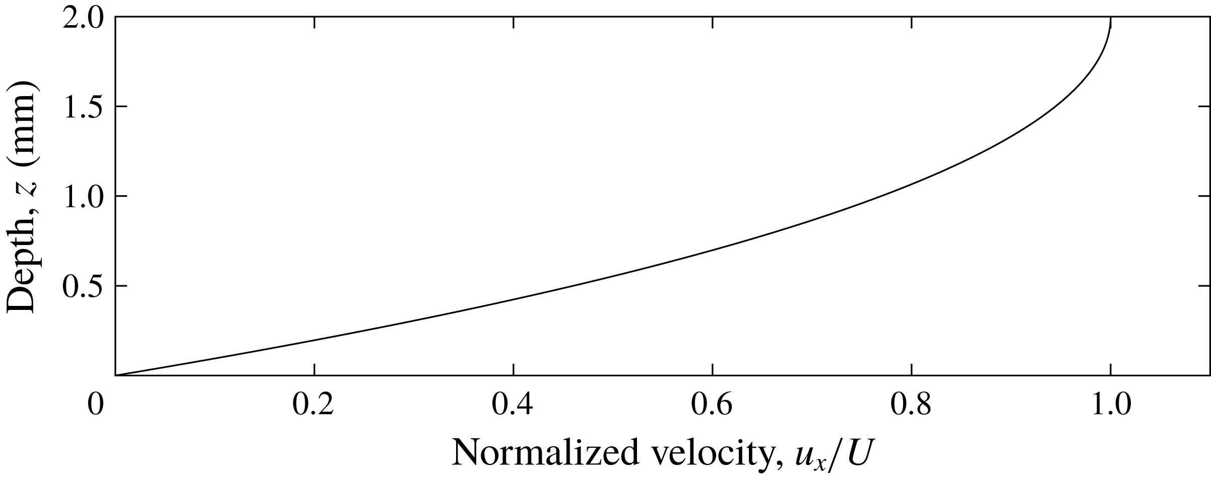
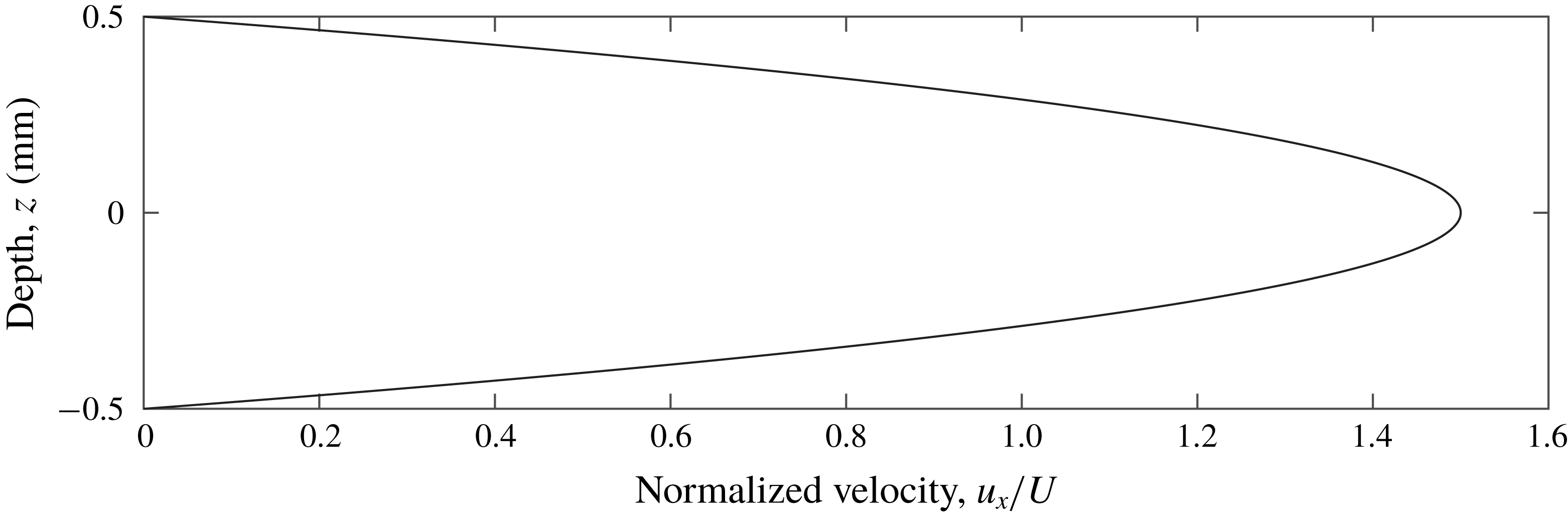
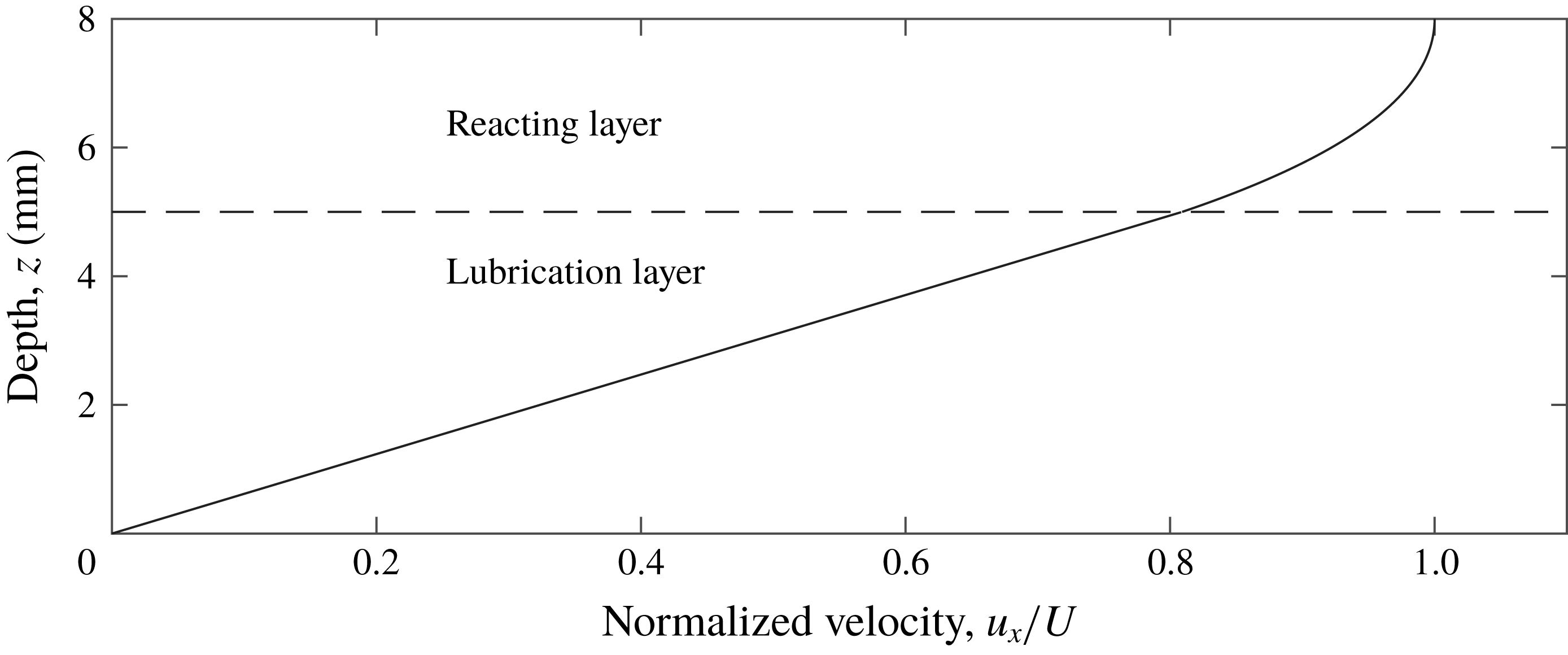
The velocity profile is shown in figure 2. At
 $z=h$
, where flow is typically measured in experiments, the velocity is
 $$\begin{eqnarray}\displaystyle \boldsymbol{u}(x,y,h)=U\hat{\boldsymbol{x}}=\frac{JB_{0}}{\unicode[STIX]{x1D707}\unicode[STIX]{x1D706}}\left(\frac{1}{\unicode[STIX]{x1D706}}-\frac{e^{-\unicode[STIX]{x1D706}h}}{\unicode[STIX]{x1D706}}-e^{-h\unicode[STIX]{x1D706}}h\right)\hat{\boldsymbol{x}}. & & \displaystyle\end{eqnarray}$$
Figure 2 and equation (2.3) make it clear that flow in these experiments will vary with depth, causing concentration to vary with depth as well.
Depth dependence of streamwise velocity in a uniform thin-layer flow.

Parameters measured from experiments and used for simulations.

2.2 Simulation
Knowing the velocity profile
 $u_{x}(z)$
, we can simulate the propagation of reaction fronts having constant chemical speed
 $v=v_{0}$
, then determine if the apparent front speed
 $v_{a}$
matches
 $v_{0}$
, as it would be if the flow
 $\boldsymbol{u}$
were independent of depth. The eikonal approximation leads to a set of ordinary differential equations governing the position and angle
 $\unicode[STIX]{x1D703}$
of a reaction front in the vertical
 $x$
–
 $z$
plane (Mitchell & Mahoney Reference Mitchell and Mahoney2012)
 $$\begin{eqnarray}\displaystyle \frac{\unicode[STIX]{x2202}x}{\unicode[STIX]{x2202}t} & = & \displaystyle u_{x}+v_{0}\sin \unicode[STIX]{x1D703},\end{eqnarray}$$
 $$\begin{eqnarray}\displaystyle \frac{\unicode[STIX]{x2202}z}{\unicode[STIX]{x2202}t} & = & \displaystyle -v_{0}\cos \unicode[STIX]{x1D703},\end{eqnarray}$$
 $$\begin{eqnarray}\displaystyle \frac{\unicode[STIX]{x2202}\unicode[STIX]{x1D703}}{\unicode[STIX]{x2202}t} & = & \displaystyle -\frac{\unicode[STIX]{x2202}u_{x}}{\unicode[STIX]{x2202}z}\sin ^{2}\unicode[STIX]{x1D703}.\end{eqnarray}$$
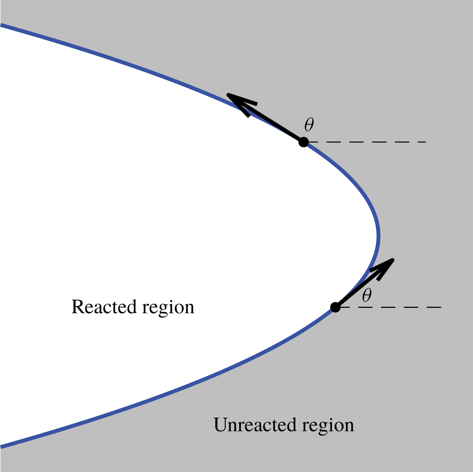
Consistent with Mitchell & Mahoney (Reference Mitchell and Mahoney2012), we define the angle,
 $\unicode[STIX]{x1D703}$
, as the angle a front element makes with the
 $x$
axis, oriented such that the front advances in the
 $\hat{\boldsymbol{n}}$
direction which makes an angle
 $\unicode[STIX]{x1D703}-\unicode[STIX]{x03C0}/2$
with the
 $x$
axis. Accordingly, a front element with
 $\unicode[STIX]{x1D703}=\unicode[STIX]{x03C0}$
is horizontal and propagates vertically with
 $\hat{\boldsymbol{n}}=\hat{\boldsymbol{z}}$
. Figure 3 shows what these variables look like those in a front simulation.
Each point on a reaction front moves in the direction that is locally normal to the front;
 $\unicode[STIX]{x1D703}$
is the angle of the tangent vector, measured counterclockwise from the
 $\hat{\boldsymbol{x}}$
direction.

There are a number of useful features of these equations. First, they mandate that front elements move with a speed that is the sum of the local flow speed and
 $v_{0}$
, a constant we choose. Second, the vertical shear
 $\unicode[STIX]{x2202}u_{x}/\unicode[STIX]{x2202}z$
appears explicitly and has the effect of changing the front angle
 $\unicode[STIX]{x1D703}$
. Equation (2.6) shows that when
 $\unicode[STIX]{x1D703}\neq \unicode[STIX]{x03C0}/2$
and
 $\unicode[STIX]{x1D703}\neq -\unicode[STIX]{x03C0}/2$
, the front element has a vertical component to its propagation. Even if
 $\unicode[STIX]{x1D703}=\unicode[STIX]{x03C0}/2$
initially for all front elements, because
 $\unicode[STIX]{x2202}u_{x}/\unicode[STIX]{x2202}z\neq 0$
, the positions and angles of front elements evolve differently over time than if they were acted on by a uniform flow of magnitude equal to the flow speed at their starting height. Third, front curvature and Ekman pumping are absent and cannot obfuscate the effect of shear on
 $v_{a}$
. Finally, it should also be noted that equations (2.5)–(2.7) are much simpler than equation (1.1) and much less demanding to solve numerically, making them a preferable tool if they accurately model experiments.
We used equations (2.5)–(2.7) to simulate reaction fronts with constant chemical speed
 $v_{0}$
in two flows: supporting flow
 $\boldsymbol{u}=u_{x}\,\hat{\boldsymbol{x}}$
as given by equation (2.3), and opposing flow
 $\boldsymbol{u}=-u_{x}\,\hat{\boldsymbol{x}}$
. Parameter values were chosen to match laboratory experiments and are listed in table 1. We initiated fronts at time
 $t=0$
with
 $x=0$
and
 $\unicode[STIX]{x1D703}=\unicode[STIX]{x03C0}/2$
for 200 front elements spaced evenly over
 $0\leqslant z\leqslant h$
. The front was advanced through time using a fourth-order Runge–Kutta method with a time step corresponding to 0.001 s. After each Runge–Kutta step, we interpolated along the front to relocate its elements at the original depths, preventing loss of resolution through the bottom and top of our domain, then recalculated
 $\unicode[STIX]{x1D703}$
from
 $x$
and
 $z$
for self-consistency.
The boundary conditions for
 $\unicode[STIX]{x1D703}$
are subtle. The concentration outside the domain is always
 $C=0$
, and the front propagation direction
 $\hat{\boldsymbol{n}}$
points in the direction of decreasing
 $C$
, by definition. Since
 $C<0$
is non-physical, a front element cannot emerge from outside the domain, but can vanish into the edge of the domain. Accordingly, we impose the boundary condition
 $-\unicode[STIX]{x03C0}/2\leqslant \unicode[STIX]{x1D703}\leqslant \unicode[STIX]{x03C0}/2$
at
 $z=0$
. In practice, the condition must be imposed only for opposing flow; supporting flow tends to rotate front elements in the allowable direction. At
 $z=h$
, the initial angle
 $\unicode[STIX]{x1D703}=\unicode[STIX]{x03C0}/2$
remains unchanged because
 $\unicode[STIX]{x2202}u_{x}/\unicode[STIX]{x2202}z=0$
there, so fronts never emerge from outside the domain. At
 $z=h$
, and in supporting flow at
 $z=0$
,
 $\unicode[STIX]{x1D703}$
is determined using a front element interpolated outside the domain.
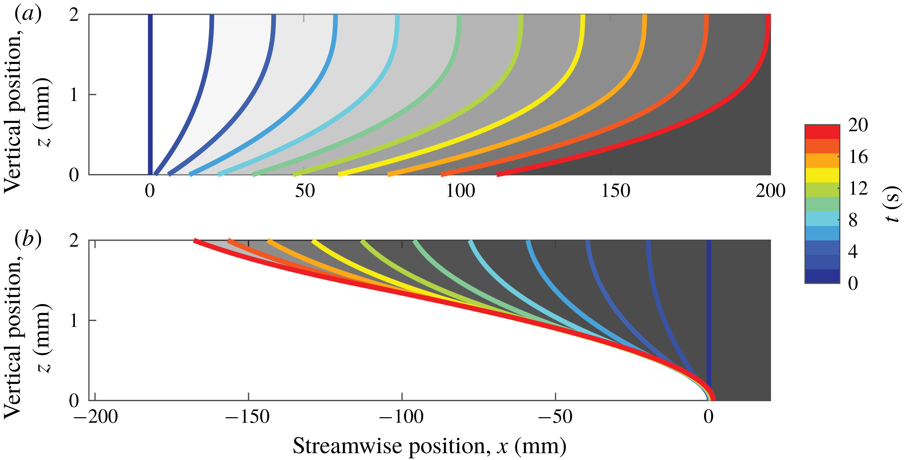
Figure 4 and supplemental movie 1 (available online at https://doi.org/10.1017/jfm.2019.460) show simulated front evolution over time. Eikonal fronts in a thin layer do not remain straight and vertical, but have positions that vary with depth, even in an entirely horizontal flow (equation (2.3)), because of shear. Also, we observe a symmetry difference between fronts in supporting flow (figure 4 a) and opposing flow (figure 4 b), which causes a change in front shape. Fronts in opposing flow are pinned at the solid boundary, maintaining a point that resists flow, whereas no such pinning occurs in supporting flows. Because they are pinned, fronts in opposing flow are sheared more strongly. This difference will result in higher apparent chemical speeds in opposing flow than supporting flow.
Fronts propagating in supporting and opposing thin-layer flow, according to the eikonal equation. Each curve represents the location of a front moving at
 $v_{0}=72~\unicode[STIX]{x03BC}\text{m}~\text{s}^{-1}$
, throughout the depth of a thin layer. Different colours indicate different times, and unreacted regions are shaded grey. Flow speed is
 $10~\text{mm}~\text{s}^{-1}$
in both cases. Fronts are initialized with
 $\unicode[STIX]{x1D703}=\unicode[STIX]{x03C0}/2$
and would propagate in the
 $\hat{\boldsymbol{x}}$
direction in the absence of flow. The flow is directed to be either (a) supporting the front (
 $\hat{\boldsymbol{x}}$
) or (b) opposing the front (
 $-\hat{\boldsymbol{x}}$
).

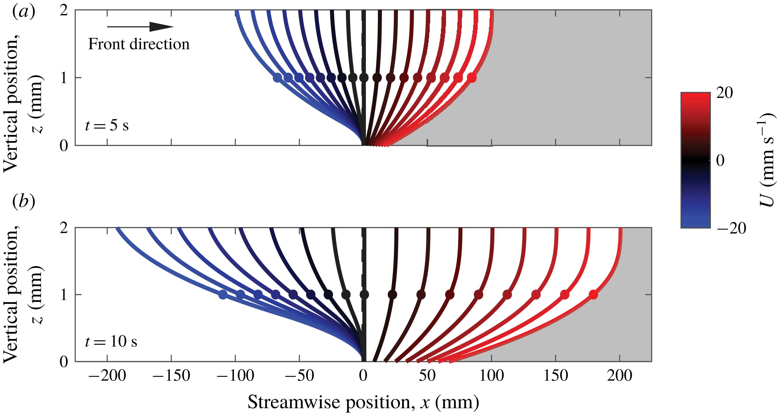
After seeing the shape of eikonal fronts change over time, we varied the flow speed. Eikonal fronts were simulated for 20 s of front growth in flows with
 $-20~\text{mm}~\text{s}^{-1}\leqslant U\leqslant 20~\text{mm}~\text{s}^{-1}$
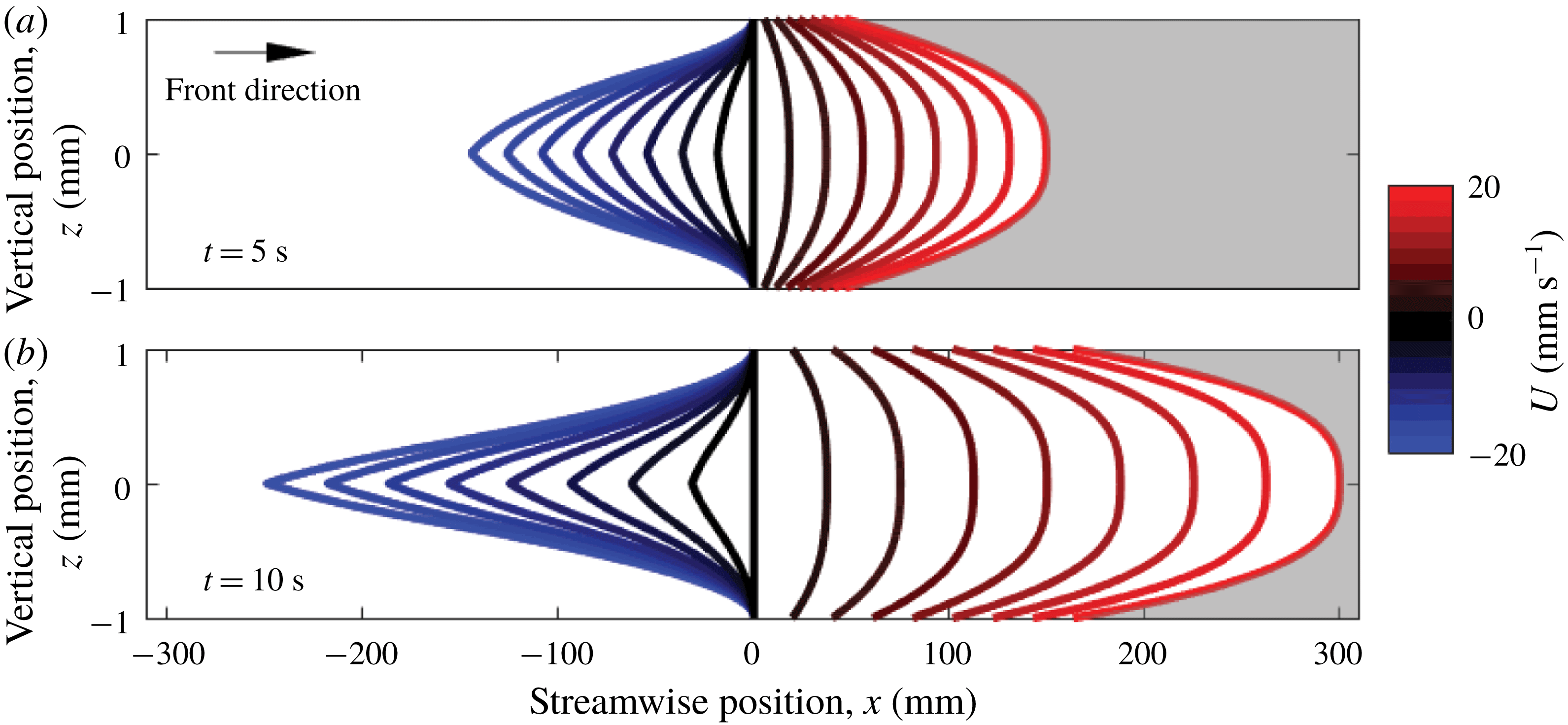
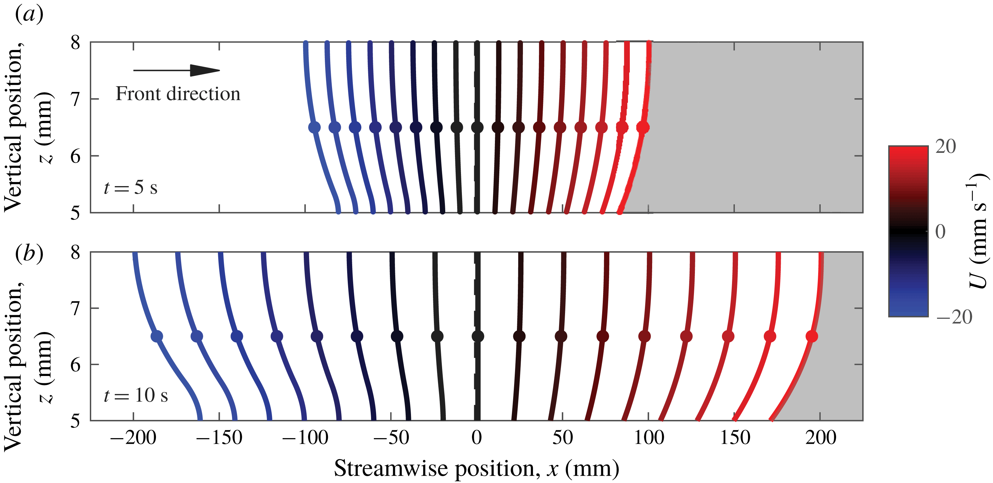
. Figure 5 shows all the fronts at two times,
 $t=5$
s and
 $t=10~\text{s}$
. As one might guess, larger flow magnitudes cause greater displacements and slopes that deviate more from vertical. Given the condition of fixed chemical speed
 $v_{0}$
in a single-layer system of fixed depth, we can focus on two important variables for fronts growing in a single layer: time and flow intensity.
Front propagation in thin-layer flow, varying with flow speed, according to the eikonal equation. Colour indicates the flow speed
 $U$
at the top surface (
 $z=h$
). The white side indicates the reacted side, and the growth direction is to the right. (a) Shows fronts after propagating 5 s, and (b) shows the same fronts after 10 s. All fronts were initialized as vertical lines at
 $x=0$
.

In order to compare to experiments, we use the depth-averaged concentration of each simulation to assign an apparent front location, as would be done in the laboratory. When fronts deviate from being strictly vertical, the depth-averaged concentration varies more gradually in space; fronts appear to be smeared by shear, as shown in supplemental movie 2. Apparent fronts can be assigned where the depth-averaged concentration crosses some user-defined threshold. For sharp, vertical fronts, the choice of threshold is irrelevant. For fronts smeared by vertical shear, the apparent front location depends on both the choice of threshold and the actual front profile. If vertical shear changes the actual front profile over time, apparent front speed is also affected. Using the results described above, we chose threshold
 $\unicode[STIX]{x1D6FE}=50\,\%$
of the maximum depth-averaged concentration to locate an apparent front at each time
 $t$
in each simulation, naming that location
 $x_{f}(t)$
. We calculated the total velocity of the apparent front
 $$\begin{eqnarray}\displaystyle \boldsymbol{w}=\frac{x_{f}(t+dt)-x_{f}(t)}{dt}\hat{\boldsymbol{x}}, & & \displaystyle\end{eqnarray}$$
where
 $dt$
is the time step. Then we calculated the apparent chemical speed
 $v_{a}$
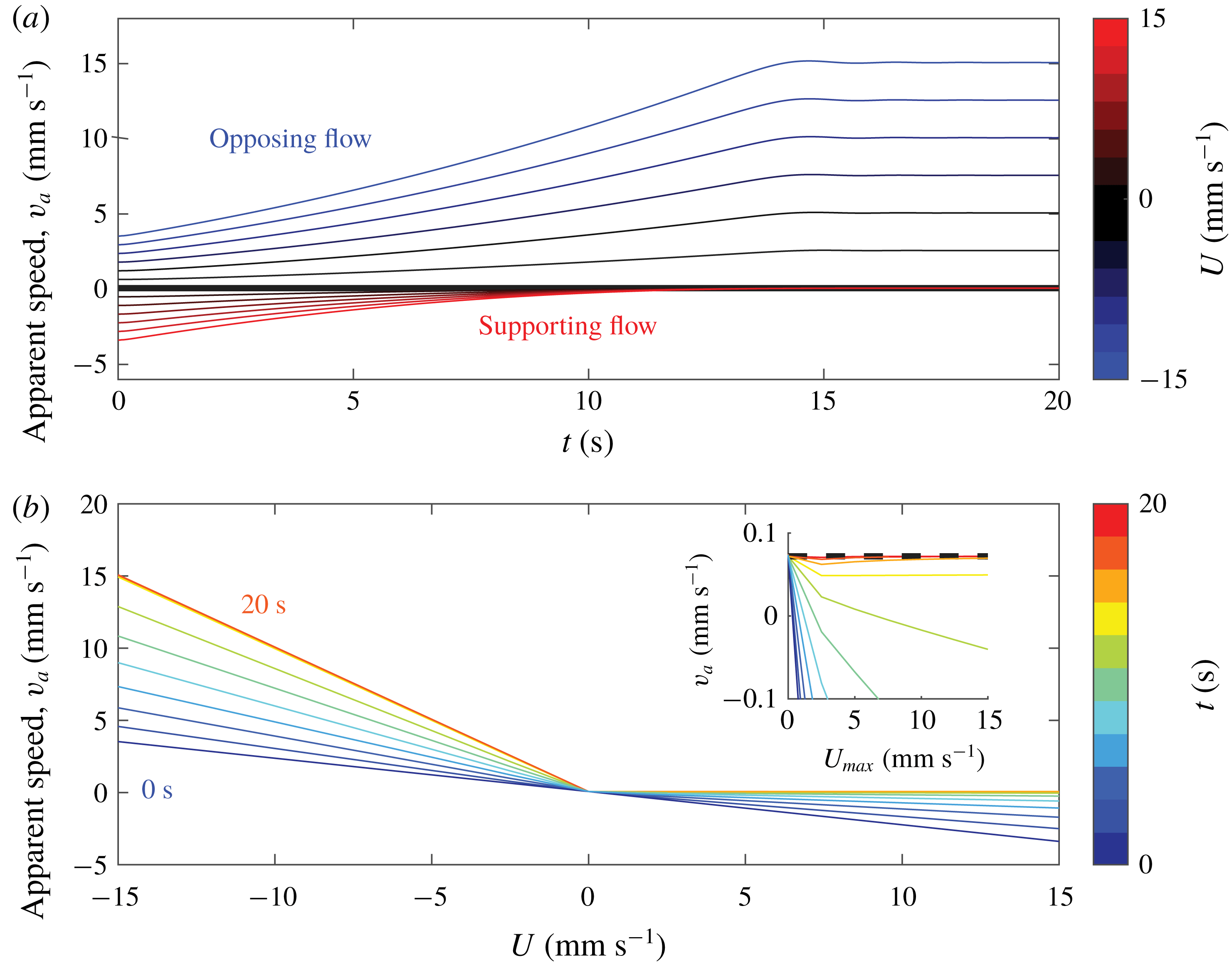
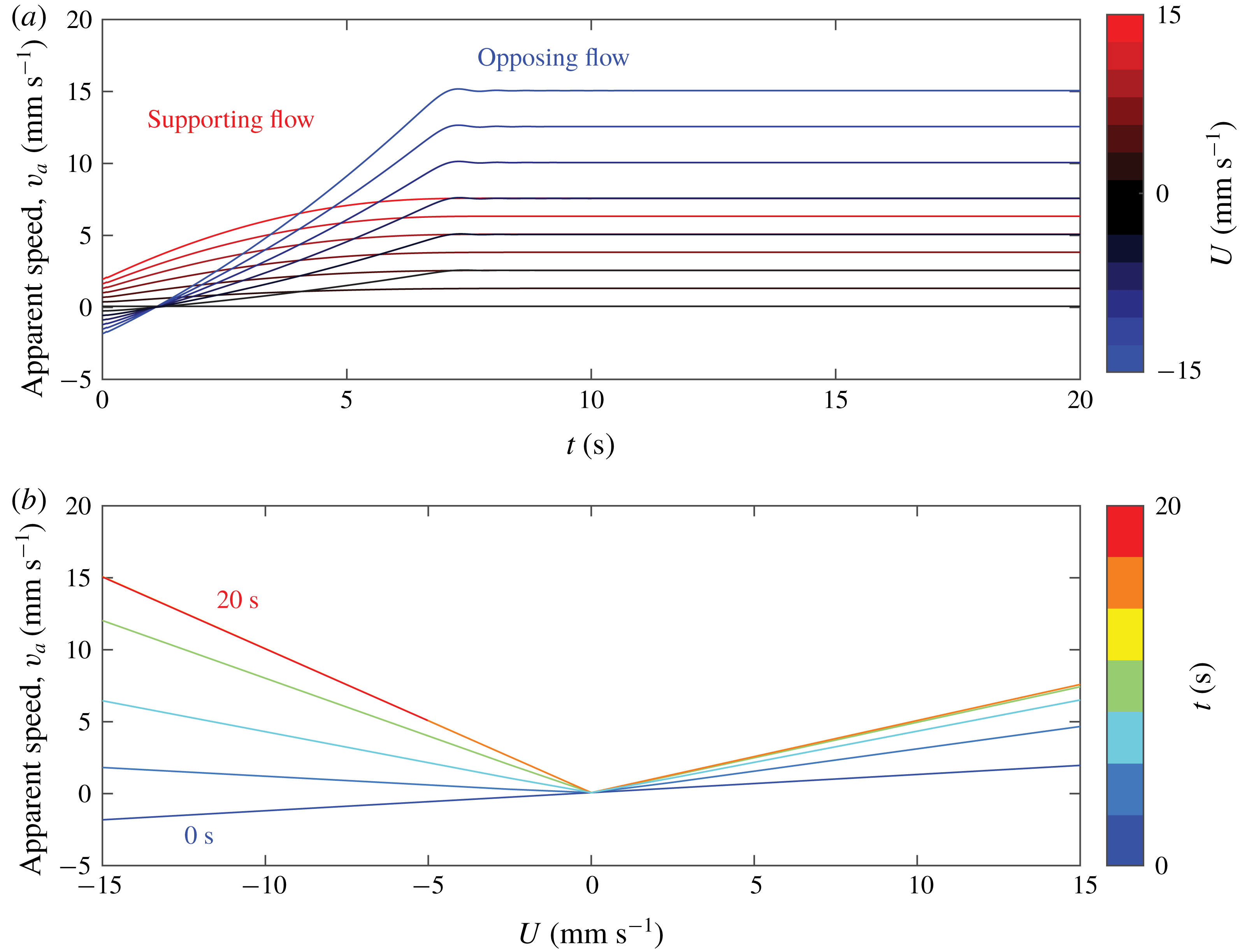
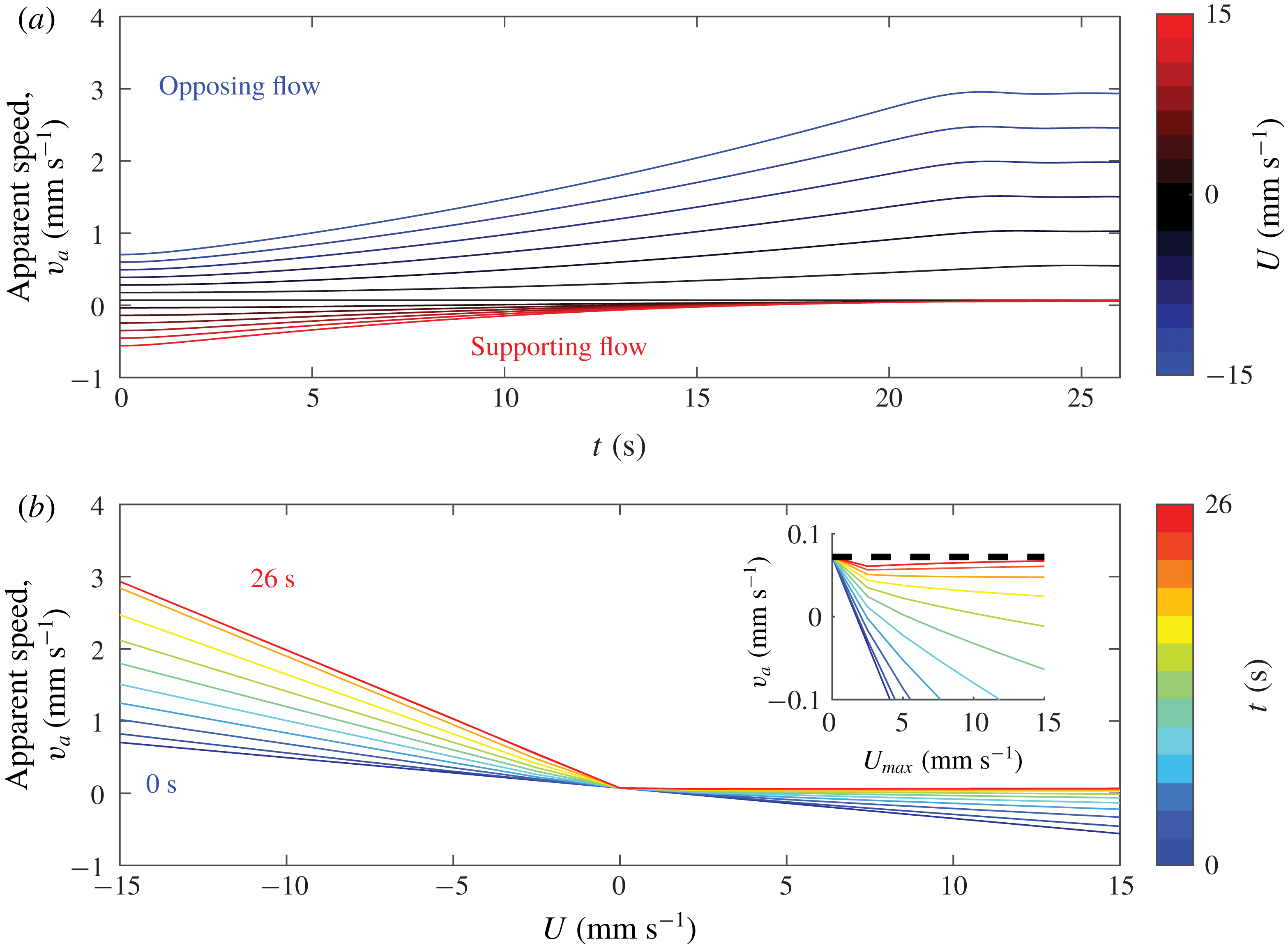
using equation (1.2) and the known flow. Figure 6 shows the results. We find that shear can cause the apparent front speed to be orders of magnitude larger than
 $v_{0}=72~\unicode[STIX]{x03BC}\text{m}~\text{s}^{-1}$
. Similar results can be found in Leconte et al. (Reference Leconte, Martin, Rakotomalala and Salin2003) for Poiseuille advection. However, those results pertain to the apparent total speed,
 $w$
, not the apparent chemical speed
 $v_{a}$
, and the focus was long-term behaviour, neglecting evolution over time.
Apparent chemical front speed in a simulated thin-layer flow, determined using depth-averaged concentration. (a) Shows apparent speed as it evolves over time, for different flow speeds. (b) Shows the variation of apparent speed with flow speed, at different times, in 2 s intervals. All chemical velocities were obtained by tracking the position where 50 % of the layer is reacted, and subtracting the flow speed at the surface, mimicking the procedures for tracking fronts in experiments. Over time, the apparent front speed converges to
 $v_{0}$
for supporting flow – as shown by the inset – and
 $v_{0}+U$
for opposing flow.

These simple simulations confirm that apparent front speeds in quasi-2-D experiments can vary and be anomalously large, even when the underlying dynamics has a constant front speed. The simulations also show that the apparent front speed converges to an asymptotic limit at long times, although the limit depends on the flow direction. For supporting flow, the apparent speed
 $v_{a}$
converges to the true chemical speed
 $v_{0}$
. For opposing flow, the apparent speed converges to
 $v_{0}+U$
, the sum of the actual chemical speed and the maximum flow speed. In either case, the apparent speed approaches the asymptotic limit from below.
Figure 6(b) suggests an explanation. At
 $t=0$
,
 $v_{a}\propto U$
with the same slope for all values of
 $U$
, but at later times,
 $v_{a}$
and
 $U$
are related by a piecewise function with two linear parts, each having a slope that evolves over time toward its asymptotic value. The initial slope can be explained by observing that at
 $t=0$
, the 50 % position has
 $\unicode[STIX]{x1D703}=\unicode[STIX]{x03C0}/2$
, so it moves perfectly in the
 $\hat{\boldsymbol{x}}$
direction. Thus for any
 $U$
, the measured front speed at
 $t=0$
will be
 $v_{a}=v_{0}+u_{x}(z=h/2)-U$
. Factoring out the surface speed and direction, the slope can be identified as
 $\tilde{u_{x}}(z=h/2)-1$
, where
 $\tilde{u_{x}}(h/2)=u_{x}(z=h/2)/U$
. Convergence of the apparent chemical speed depends on the concentration profile converging to its long-term shape (figure 4), which occurs as information propagates at the true chemical speed across the layer depth, starting at the leading edge of the front and finally reaching the depth
 $\unicode[STIX]{x1D6FE}h$
. The process is analogous to the downstream widening of a boundary layer or narrowing of an entrance region in pipe flow. Opposing fronts have leading edges at the bottom of the layer, so they converge to the speed of the front at the bottom, which is
 $v_{a}=v_{0}$
. Their characteristic time for convergence is
 $\unicode[STIX]{x1D70F}_{o}=\unicode[STIX]{x1D6FE}h/v_{0}$
. Supporting fronts have leading edges at the top of the layer, so they converge to the velocity at the surface, which is
 $v_{a}=(v_{0}+U)$
. Their characteristic time for convergence is
 $\unicode[STIX]{x1D70F}_{s}=(1-\unicode[STIX]{x1D6FE})h/v_{0}$
. In the case of
 $\unicode[STIX]{x1D6FE}=0.5$
, both convergence times are the same, and for the parameters listed in table 1,
 $\unicode[STIX]{x1D70F}_{o}=\unicode[STIX]{x1D70F}_{s}=13.9$
s. Choosing
 $\unicode[STIX]{x1D6FE}<0.5$
results in faster convergence for opposing fronts than for supporting fronts; choosing
 $\unicode[STIX]{x1D6FE}>0.5$
results in faster convergence for supporting fronts. The convergence time does not depend on flow speed or structure. The value of
 $\unicode[STIX]{x1D6FE}$
does not change the asymptotic apparent chemical speed.
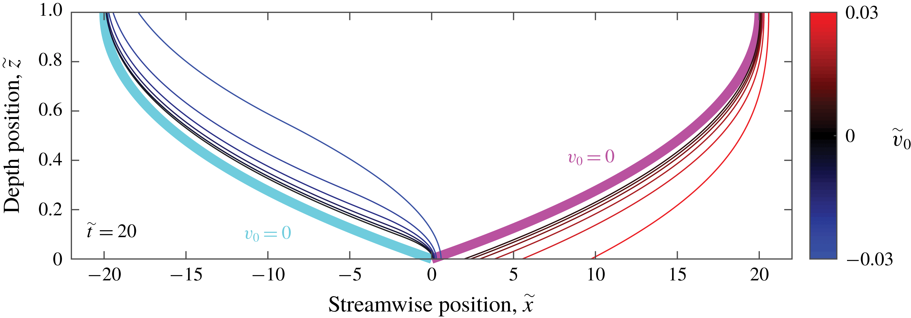
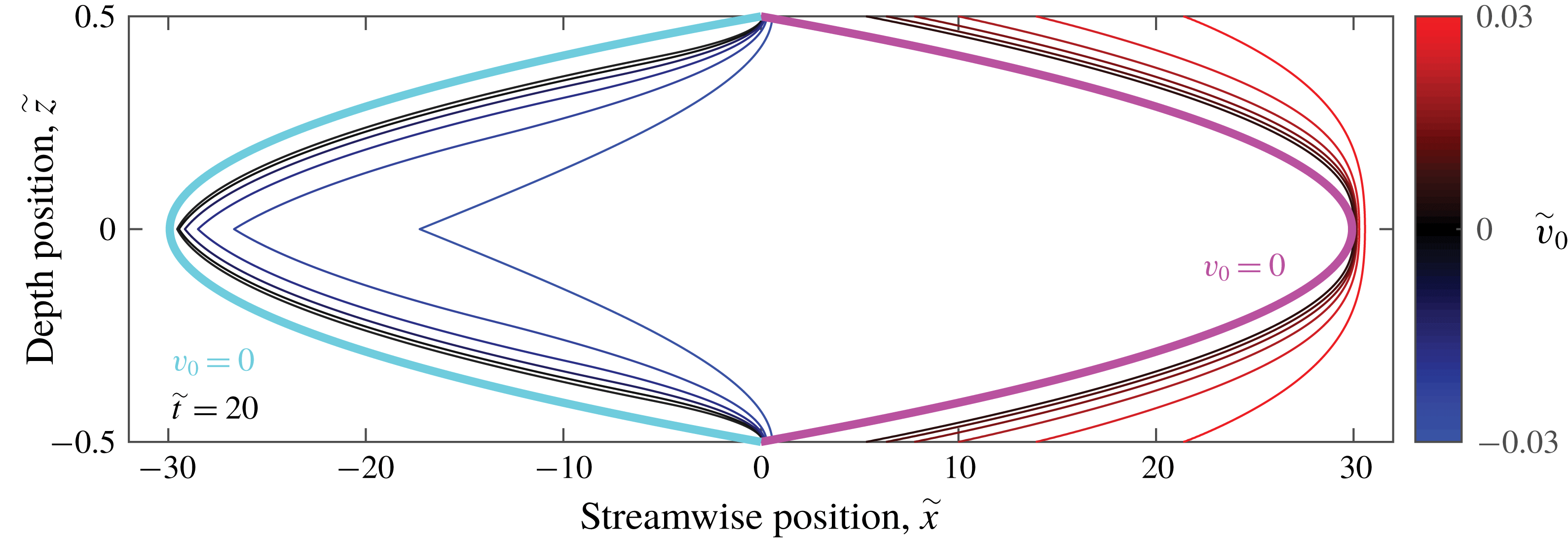
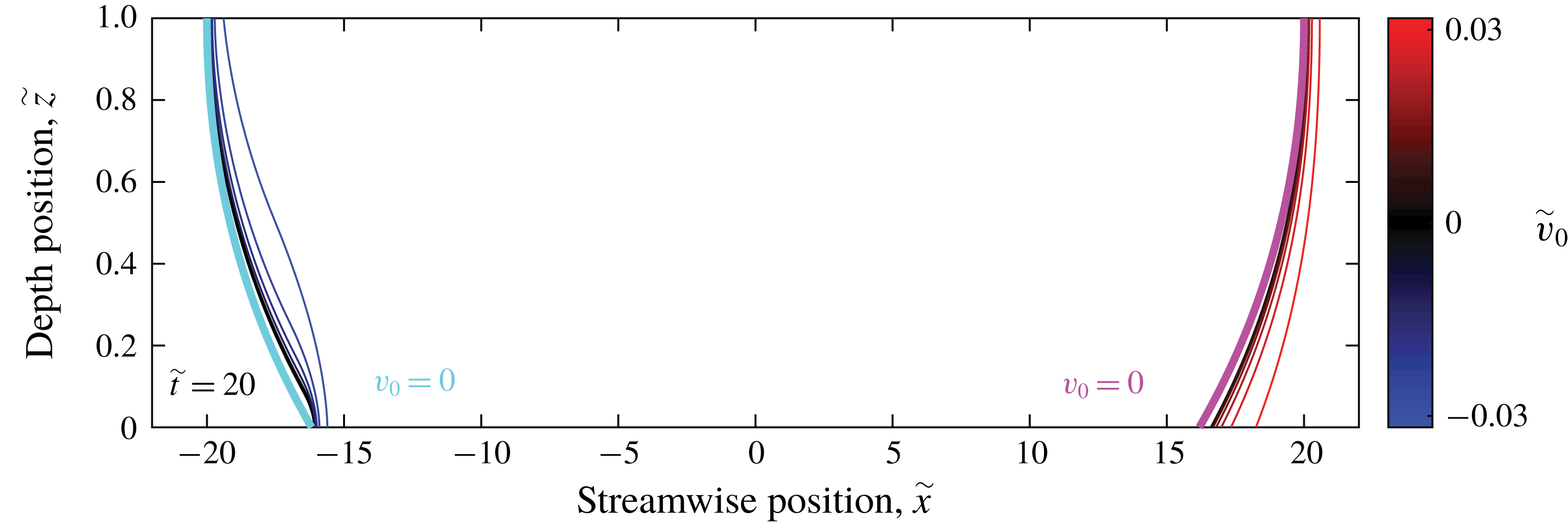
Further insight can be gained if we consider front propagation in dimensionless form. Normalizing simulation results like those shown in figure 5 with velocity scale
 $U$
, length scale
 $h$
, and time scale
 $h/U$
produces the dimensionless front profiles shown in figure 7. The simulations plotted there differ only in the ratio
 $\tilde{v_{0}}=v_{0}/U$
. When
 $|\tilde{v_{0}}|$
is large, the front propagates further in the
 $\hat{\boldsymbol{x}}$
direction and extends across a shorter region (in dimensionless units): fronts are less distorted by vertical shear. On the other hand, when
 $|\tilde{v_{0}}|$
is small, fronts converge to the shapes we would expect in passive scalar mixing. The curves for a non-reactive scalar are also mirror images of each other, because the front has no directionality in the
 $\tilde{v_{0}}=0$
case. Front speed is what breaks the symmetry between supporting and opposing flows. Although flow speeds in our experiments (described in § 5) are often much faster than reaction front speeds, we nonetheless observe clear deviation from the
 $\tilde{v_{0}}=0$
case.
Front propagation in thin-layer flow, varying with front speed
 $v_{0}/U$
, normalized with the flow speed
 $U$
and the layer depth
 $h$
, at dimensionless time
 $\tilde{t}=20$
. As
 $v_{0}/U$
decreases, the fronts approach the passive case for both opposing and supporting flows.

3 Simulations of Hele-Shaw system
Another common configuration for thin-layer flow experiments involves a single reacting layer between two solid boundaries, driven by a pressure difference (Sharif, Abid & Ronney Reference Sharif, Abid and Ronney1999; Atis et al. Reference Atis, Saha, Auradou, Salin and Talon2013; Chevalier et al. Reference Chevalier, Salin and Talon2017). One major advantage of that configuration, often called a Hele-Shaw system, is that the reacting layer can be made much thinner than in free-surface systems. However, the resulting no-slip conditions on both the top and bottom of the layer cause much stronger shear for the same layer thickness. Regardless, in many systems where a free surface is impractical, the Hele-Shaw configuration is the only option. As with thin-layer experiments, the vertical shear will have an effect, and here we attempt to quantify that effect.
3.1 Velocity profile
Flow in a Hele-Shaw system is driven by a pressure difference
 $\unicode[STIX]{x1D735}P$
with no-slip boundary conditions at
 $z=\pm h/2$
. Solving equation (2.1) results in Poiseuille flow. If the flow is in the
 $\hat{\boldsymbol{x}}$
direction, then the velocity profile is parabolic,
 $$\begin{eqnarray}\displaystyle u_{x}(z)=\unicode[STIX]{x1D735}P\,\frac{z^{2}-(h/2)^{2}}{2\unicode[STIX]{x1D707}}, & & \displaystyle\end{eqnarray}$$
as shown in figure 8. The profile is symmetric about
 $z=0$
, and the lower half has the same form as the single-layer profile shown in figure 2. The other major difference between single-layer experiments and Hele-Shaw experiments is in how flow speed is measured. Since particles cannot float on the surface of a Hele-Shaw system, the average flow speed through the depth is frequently used instead. Since this is the flow speed of interest, we will define
 $U$
to be equal to this average. Integration of equation (3.1) yields
 $$\begin{eqnarray}\displaystyle U=-\unicode[STIX]{x1D735}P\frac{h^{2}}{12\unicode[STIX]{x1D707}}. & & \displaystyle\end{eqnarray}$$
If we instead defined
 $U=u_{x}(z=0)$
, the results would be essentially indistinguishable from those of a single-layer system with layer thickness
 $h/2$
.
Depth dependence of streamwise velocity in a Hele-Shaw style, pressure-driven flow. Fluid properties and layer thicknesses are given in table 1, with
 $\unicode[STIX]{x1D735}P$
set to normalize the maximum speed.

3.2 Simulation
We repeated the simulations described in § 2.2 with
 $u_{x}$
given by equation (3.1), increasing the values of
 $\unicode[STIX]{x1D735}P$
so that values of
 $U$
fall in the same range as before. Fronts from simulations with different
 $U$
values are presented in figure 9. The two no-slip boundaries enhance the differences between fronts in supporting and opposing flow. Fronts in opposing flow now pin to both the top and the bottom of the domain, whereas the trailing edge of the front occurs at the centre of the layer. A sharp cusp forms there on fronts in opposing flow, whereas fronts in supporting flow are not only smooth at the centre of the layer, but flattened there.
Front propagation in the Hele-Shaw system, varying with flow speed, according to the eikonal equation. Colour indicates the flow speed
 $U$
equal to the average flow speed throughout the depth. The white side indicates the reacted side, and the growth direction is to the right. (a) Shows fronts after propagating 5 s, and (b) shows the same fronts after 10 s. All fronts were initialized as vertical lines at
 $x=0$
.

As with the single layer, the apparent chemical front speed
 $v_{a}$
shows strong deviation from
 $v_{0}$
. Figure 10 shows apparent front speeds at different flow speeds and times. The shapes of the plotted curves differ from single-layer systems with a free boundary. This difference arises entirely from defining
 $U$
as the average speed, which is lower than the maximum flow speed in the layer. If
 $U$
is defined as the maximum speed, these results differ from the single layer results only in the convergence time of
 $v_{a}$
. In the case of supporting flow,
 $v_{a}$
converges to
 $v_{0}-U+u_{x}(z=0)$
because the leading edge in supporting flows is at
 $u_{x}(z=0)\neq U$
. In the previous section the flow velocity at this leading edge was
 $U$
, and thus supporting flow converged to
 $v_{0}$
. The convergence time changes in Hele-Shaw because information propagates both up and down:
 $\unicode[STIX]{x1D70F}_{s}=(1-\unicode[STIX]{x1D6FE})h/2v_{0}=6.94$
s for these parameters. In the case of opposing flow,
 $v_{a}$
converges to
 $v_{0}+U$
as it did in single layer. The convergence time for opposing flow is analogous to the single-layer system:
 $\unicode[STIX]{x1D70F}_{o}=\unicode[STIX]{x1D6FE}h/2v_{0}=6.94$
s for these parameters. The initial slope of
 $v_{a}$
versus
 $U$
in the Hele-Shaw system has the opposite sign and is less steep than in the single-layer system:
 $\tilde{u_{x}}(z=h/2)-1=0.13$
instead of -0.23 for a single layer with a free surface. However, the convergence times are strictly smaller, implying that the effects of depth shear are at least as severe in Hele-Shaw systems as they are in single-layer systems, and using an average flow speed does not cause the measurement of front speed to match the expected value
 $v_{0}$
.
Apparent chemical front speed in simulated Hele-Shaw flow, determined using depth-averaged concentration. (a) Shows apparent speed as it evolves over time, for different flow speeds. (b) Shows the variation of apparent speed with flow speed, at different times, at 2 s intervals. All chemical velocities were obtained by tracking the position where 50 % of the layer is reacted, and subtracting the average flow speed, mimicking the procedures for front tracking experiments. Over time, the apparent front speed converges to
 $v_{0}-U+u_{x}(z=0)$
for supporting flow and
 $v_{0}+U$
for opposing flow.

Figure 11 shows front propagation in dimensionless form for the Hele-Shaw system. We still see the cusp formation in the dimensionless system. Fronts in the Hele-Shaw system are around 60 times wider than tall, whereas fronts in the single-layer system are around 20 times wider than tall. This difference is in large part due to the fact that a Hele-Shaw layer of the same thickness as a single layer must reach its maximum speed in half the distance due to the reflection across the
 $x$
axis.
Front propagation in the Hele-Shaw system, varying with front speed
 $v_{0}/U$
, normalized with the flow speed
 $U$
and the layer depth
 $h$
, at dimensionless time
 $\tilde{t}=20$
. As
 $v_{0}/U$
decreases, the fronts approach the passive case for both opposing and supporting flows.

4 Simulations of two-layer system
As we showed in § 2, shear in thin-layer flows changes the apparent chemical front speed, if it is measured using depth-averaged concentration, even in simulations that exclude higher-order mechanisms like curvature and Ekman pumping. Section 3 showed that shear can also change the results of a Hele-Shaw style experiment. Studies of front propagation with thin-layer experiments must therefore be undertaken with care. To ensure that the apparent front speed gives a good approximation for the true front speed, shear must be minimized. One strategy for minimizing shear is to add an immiscible, dielectric lubrication layer below the reacting layer. In this section we will repeat the analysis and simulation of § 2 for such a two-layer system. We will show that the two-layer system produces apparent front speeds much closer to the true front speed, although shear still has some effect.
4.1 Velocity profile
To determine the velocity profile of the two-layer system, we must consider each layer separately. In the lubrication layer that occupies the region
 $0\leqslant z\leqslant h_{d}$
, current cannot flow:
 $J=0$
. In the reacting layer that occupies the region
 $h_{d}\leqslant z\leqslant h_{d}+h_{e}=h$
, the current density is unchanged from the single-layer case. Flow at the interface between the layers must be continuous and stress free, so the boundary conditions at
 $h_{d}$
require that
 $u_{x}$
be continuous and
 $$\begin{eqnarray}\displaystyle \left.\unicode[STIX]{x1D707}_{d}\frac{\unicode[STIX]{x2202}u_{x}}{\unicode[STIX]{x2202}z}\right|_{h_{d}^{-}}=\unicode[STIX]{x1D707}\left.\frac{\unicode[STIX]{x2202}u_{x}}{\unicode[STIX]{x2202}z}\right|_{h_{d}^{+}}, & & \displaystyle\end{eqnarray}$$
where
 $\unicode[STIX]{x1D707}_{d}$
and
 $\unicode[STIX]{x1D707}$
are the viscosities of the lubrication layer and reacting layer, respectively, and
 $h_{d}^{-}$
 $h_{d}^{+}$
indicate locations infinitesimally below and above
 $z=h_{d}$
, respectively. Other parameters and boundary conditions remain unchanged. Solving equation (2.1), we find
 $$\begin{eqnarray}\displaystyle u_{x}(z)=\left\{\begin{array}{@{}ll@{}}\displaystyle \frac{JB_{0}z}{\unicode[STIX]{x1D707}_{d}\unicode[STIX]{x1D706}}e^{-\unicode[STIX]{x1D706}h_{d}}(1-e^{-\unicode[STIX]{x1D706}h_{e}}),\quad & 0\leqslant z\leqslant h_{d},\\ \displaystyle \frac{JB_{0}}{\unicode[STIX]{x1D707}\unicode[STIX]{x1D706}}\left(h_{d}e^{-\unicode[STIX]{x1D706}h_{d}}\left[\frac{\unicode[STIX]{x1D707}}{\unicode[STIX]{x1D707}_{d}}-\frac{\unicode[STIX]{x1D707}}{\unicode[STIX]{x1D707}_{d}}e^{-\unicode[STIX]{x1D706}h_{e}}+\frac{1}{\unicode[STIX]{x1D706}h_{d}}+e^{-\unicode[STIX]{x1D706}h_{e}}\right]\right.\quad & \\ \displaystyle \left.\qquad \qquad -\,\frac{e^{-\unicode[STIX]{x1D706}z}}{\unicode[STIX]{x1D706}}-ze^{-\unicode[STIX]{x1D706}(h_{d}+h_{e})}\right),\quad & h_{d}\leqslant z\leqslant h_{d}+h_{e}.\end{array}\right. & & \displaystyle\end{eqnarray}$$
This velocity profile agrees closely with the results of Suri et al. (Reference Suri, Tithof, Mitchell, Grigoriev and Schatz2014), with differences arising from our use of an exponentially decaying magnetic field (equation (2.2)); they used a linear decay. Figure 12 shows the velocity profile for the parameters shown in table 1. Because
 $\unicode[STIX]{x1D707}\sim \unicode[STIX]{x1D707}_{d}$
, the slope discontinuity (kink) at
 $z=h_{d}$
is weak. We define
 $U$
in a two-layer system to be the velocity at
 $z=h_{d}+h_{e}$
. As expected, only a small fraction of the vertical variation in velocity, approximately 20 %, occurs in the reacting layer.
Depth dependence of streamwise velocity in a uniform thin-layer flow including a lubrication layer. Fluid properties and layer thicknesses are given in table 1, with
 $J$
set to normalize the maximum speed.

4.2 Simulation
We repeated the simulations described in § 2.2 with
 $u_{x}$
given by equation (4.2), increasing the values of
 $J$
so that values of
 $U$
fall in the same range as before. Fronts at different
 $U$
values are presented in figure 13 and Supplemental Movie 1. Fronts in the two-layer system are distorted by vertical shear much less than fronts in the single-layer system. The asymmetry between fronts in supporting and opposing flow is smaller in two-layer systems because the bottom of the reacting layer is no longer subject to a no-slip boundary condition, so pinning is eliminated. Some asymmetry remains, however, because front elements can vanish into the edge of the domain but not emerge from it (see § 2).
Front propagation in the two-layer system, varying with flow speed, according to the eikonal equation. Colour indicates the flow speed
 $U$
at the top surface (
 $z=h_{d}+h_{e}$
). The white side indicates the reacted side, and the growth direction is to the right. (a) Shows fronts after propagating 5 s, and (b) shows the same fronts after 10 s. All fronts were initialized as vertical lines at
 $x=0$
.

This reduction of distortion has a major effect on the apparent chemical front speed
 $v_{a}$
. Figure 14 shows apparent front speeds at different flow speeds and times. The shapes of the plotted curves closely resemble those of the single-layer system (figure 5). However, the magnitude of
 $v_{a}$
for any given flow speed
 $U$
is only approximately 20 % as large as in the single-layer system. For example, the initial slope is once again equal to
 $\tilde{u_{x}}(z=h/2)-1$
, but the value is
 $-0.23$
for the single-layer system and
 $-$
0.04 for the two-layer system. Therefore there is less dependence of apparent chemical speed on flow speed in the two-layer system than in the single-layer system. In the case of supporting flow,
 $v_{a}$
converges to
 $v_{0}$
, just as in the single-layer system. The convergence time is analogous:
 $\unicode[STIX]{x1D70F}_{s}=(1-\unicode[STIX]{x1D6FE})h_{e}/v_{0}$
, which gives
 $\unicode[STIX]{x1D70F}_{s}=20.8~\text{s}$
for these parameters. In the case of opposing flow,
 $v_{a}$
does not converge to
 $v_{0}+U$
, as in the single-layer system, but to
 $v_{0}+U-u_{x}(z=h_{d})$
. That is, the apparent chemical speed exceeds the true chemical speed by the difference in flow speed at top and bottom. The same is true for the single-layer system, since the flow speed at the bottom of a single layer is zero. The convergence time for opposing flow in the two-layer system is analogous to the single-layer system:
 $\unicode[STIX]{x1D70F}_{o}=\unicode[STIX]{x1D6FE}h_{e}/v_{0}$
, which is also 20.8 s for these parameters.
Apparent chemical front speed in simulated two-layer flow, determined using depth-averaged concentration. (a) Shows apparent speed as it evolves over time, for different flow speeds. (b) Shows the variation of apparent speed with flow speed, at different times, at 2 s intervals. All chemical velocities were obtained by tracking the position where 50 % of the layer is reacted, and subtracting the flow speed at the surface, mimicking the procedures for front tracking experiments. Over time, the apparent front speed converges to
 $v_{0}$
for supporting flow – as shown by the inset – and
 $v_{0}+U-u_{x}(z=h_{d})$
for opposing flow. The apparent and true front speeds match more closely than in the single-layer configuration.

We can also consider front propagation in dimensionless form in the two-layer system, as shown in figure 15. As in the single-layer system, fronts are distorted least when
 $\tilde{v_{0}}$
is large, and have shapes like fronts bounding a passive scalar when
 $\tilde{v_{0}}$
is small. The effect of changing
 $\tilde{v_{0}}$
is much weaker than in the single-layer system, however. Fronts in the two-layer system are never more than 4 times as wide as they are tall, whereas fronts in the single-layer system can be 20 times as wide as tall.
Front propagation in the two-layer system, varying with front speed
 $\tilde{v_{0}}=v_{0}/U$
, normalized with the flow speed
 $U$
and the layer depth
 $h_{e}$
, at dimensionless time
 $\tilde{t}=20$
. As
 $\tilde{v_{0}}$
decreases, the fronts approach the passive case for both opposing and supporting flows. However, changing
 $\tilde{v_{0}}$
has a much smaller effect than in the single-layer system (figure 7) because fronts are not pinned by a no-slip boundary condition at the bottom of the layer.

5 Experimental apparatus
Our simulations show that vertical shear causes the apparent front speed
 $v_{a}$
to deviate from the true front speed
 $v_{0}$
in thin-layer experiments, assuming that the eikonal approximation (equation (1.2)) holds and that reaction fronts propagate according to equations (2.5), (2.6) and (2.7). We expect those assumptions to hold in the limit of thin fronts, when the characteristic reaction rate is much faster than the characteristic rates of advection and diffusion. That is, we expect those assumptions to hold when the first Damköhler number
 $Da_{I}=\unicode[STIX]{x1D6FC}h/U$
and second Damköhler number
 $Da_{II}=\unicode[STIX]{x1D6FC}h^{2}/D$
are both large. We find
 $Da_{II}\geqslant 2600\gg 1$
for all simulations described above, satisfying the necessary condition. However, for some simulations
 $Da_{I}=0.17$
and the validity of the assumptions is not obvious. To test the validity, and determine whether the resulting simulations accurately predict the effect of shear on apparent front speed, we performed reactive mixing experiments in thin-layer flows.
Experiments were configured to match parameters in table 1. We drove flows that were nearly uniform and nearly unidirectional by passing electrical current through a thin layer of reacting fluid in the presence of a magnetic field that varied little in the horizontal directions and decayed exponentially in the vertical direction. We varied
 $u_{x}$
by changing the current amplitude
 $J$
. All flows were steady after an initial transient. We performed experiments both with and without a lubrication layer below the reacting fluid. We did not perform Hele-Shaw experiments, however.
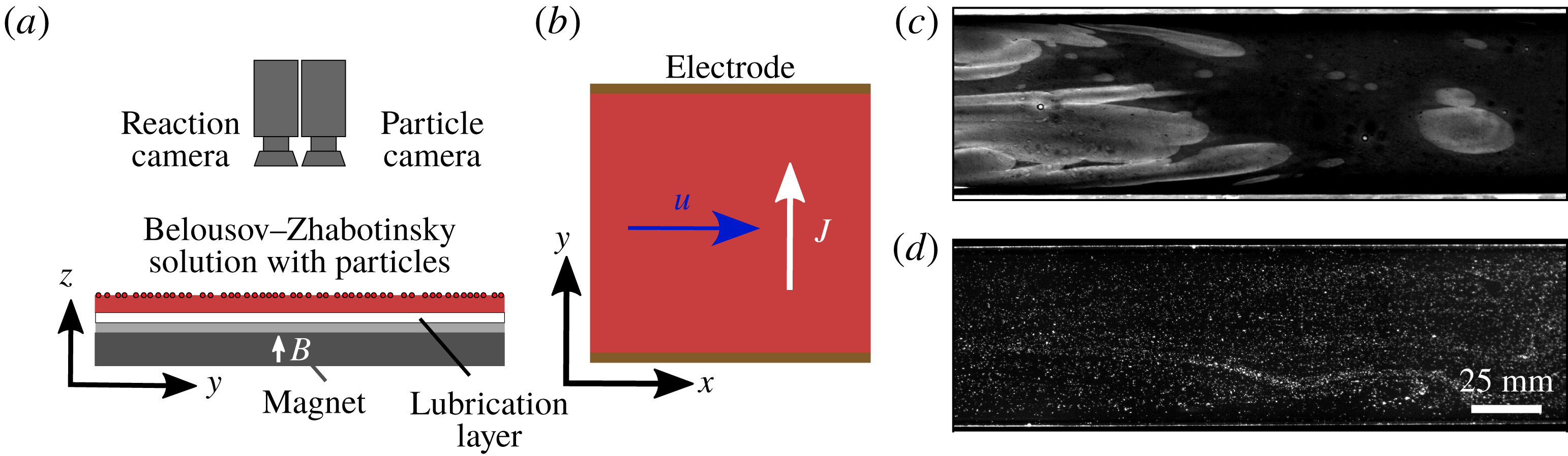
To accurately measure the dynamics of reactive mixing, we use an experimental apparatus which can measure both depth-averaged concentration and flow velocity simultaneously, as shown in figure 16. A pair of cameras (Emergent HS-4000M) images a thin layer of the reacting Belousov–Zhabotinsky (BZ) solution (Zaikin & Zhabotinsky Reference Zaikin and Zhabotinsky1970; Wood & Ross Reference Wood and Ross1985; Esptein Reference Esptein1987; Scott Reference Scott1994). It changes colour from blue to red as it reacts, producing fronts with chemical speed
 $v_{0}=72~\unicode[STIX]{x03BC}\text{m}~\text{s}^{-1}$
(Nevins & Kelley Reference Nevins and Kelley2017). Single-layer experiments were recorded with spatial resolution
 $0.163~\text{mm}~\text{pixel}^{-1}$
; two-layer experiments,
 $0.140~\text{mm}~\text{pixel}^{-1}$
. On top of the reacting layer, red fluorescent tracer particles (Cospheric UVPMS-BR-0.995,
 $75{-}90~\unicode[STIX]{x03BC}\text{m}$
) follow the flow closely, with Stokes number
 $St<0.1$
. The rectangular flow channel is 263 mm long, and its width can be varied from 59 to 68 mm wide. It is placed above a large ceramic magnet (152 mm
 $\times$
102 mm) which provides unidirectional flow down the channel. Fluid recirculates outside the viewing area (figure 16
b). In the two-layer system, immiscible Fluorinert FC-3283 is placed below the reacting layer. We illuminate the apparatus with blue LED light, which passes through the BZ solution to reflect off a white background and which matches the absorption wavelength of the particles. One camera has a blue-pass optical filter to see the light reflected from the blue reacted regions, and the other has a red-pass filter which sees the fluorescent particles; figure 16(c,d) shows examples.
The BZ reaction is an excitable redox reaction catalyzed by ferroin indicator. The reaction oscillates, allowing the same batch to be used for several different experiments. While the BZ reaction is chemically complex, we measure only the early stages of the reaction within each experiment so it is well modelled as a second-order autocatalytic reaction (Scott Reference Scott1994; Nevins & Kelley Reference Nevins and Kelley2017):
 $F(c)=c(1-c)$
. We produce the BZ solution using a recipe similar to one described previously (Bargteil & Solomon Reference Bargteil and Solomon2012). In a fume hood, we mix an aqueous solution composed of sulfuric acid (
 $\text{H}_{2}\text{SO}_{4}$
, 0.22 M), malonic acid (
 $\text{C}_{3}\text{H}_{4}\text{O}_{4}$
, 0.12 M), sodium bromide (NaBr, 0.12 M) and sodium bromate (
 $\text{NaBrO}_{3}$
, 0.34 M). A silver wire is immersed in the BZ layer for 20 s to catalyze the reaction, which is allowed to grow for 30 s before flow is started. The wire is inserted vertically to ensure that the initial front is nearly uniform throughout the layer depth, and because we want our procedures to be consistent with prior experimental studies, which have often inserted wires vertically (Nevins & Kelley Reference Nevins and Kelley2018). The resulting front spreads in a nearly circular shape, so the front propagation direction and flow direction are not aligned in most regions. By measuring both the front velocity and the flow velocity, we can readily determine the magnitude of the normal flow. Ferroin indicator is added repeatedly throughout experiments to maintain strong contrast, which would otherwise fade over the 2–3 h in which a batch of solution continues reacting. Thus colour does not provide a calibrated measurement of depth-averaged concentration, nor is it accurate to make quantitative comparisons between colour at one time and colour at a much later time. However, spatial colour variation in an image does accurately locate reaction fronts.
Diagram of the experimental apparatus. (a) Two cameras image a thin layer of reacting Belousov–Zhabotinsky solution with red tracer particles. For single-layer experiments there is no lubrication layer. (b) Flow is driven by a current in the
 $+\hat{\boldsymbol{y}}$
direction, and a magnetic field in the
 $+\hat{\boldsymbol{z}}$
direction, resulting in a channel flow in the
 $+\hat{\boldsymbol{x}}$
direction. (c) Typical image from the reaction camera, and (d) from the particle camera (inverted to enhance visibility). We use particle tracking to measure flow velocity and front tracking to measure front speeds.

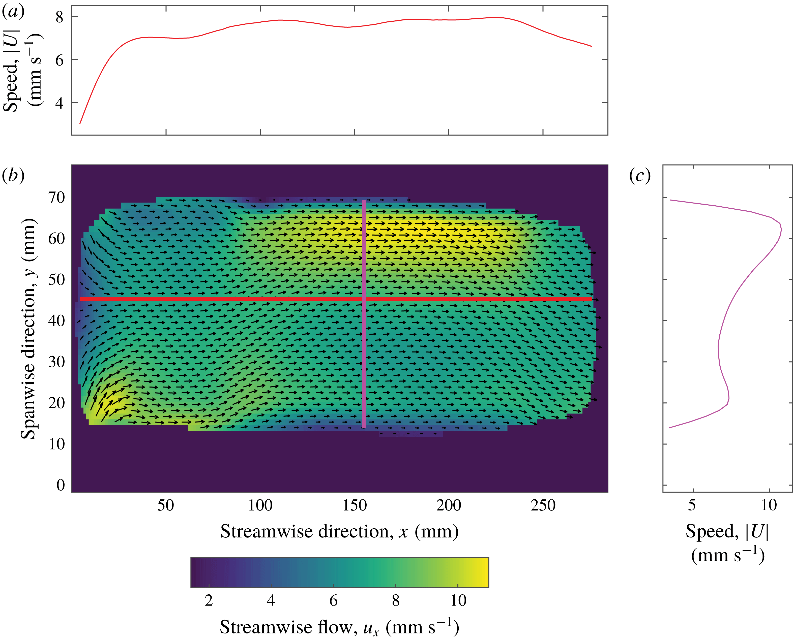
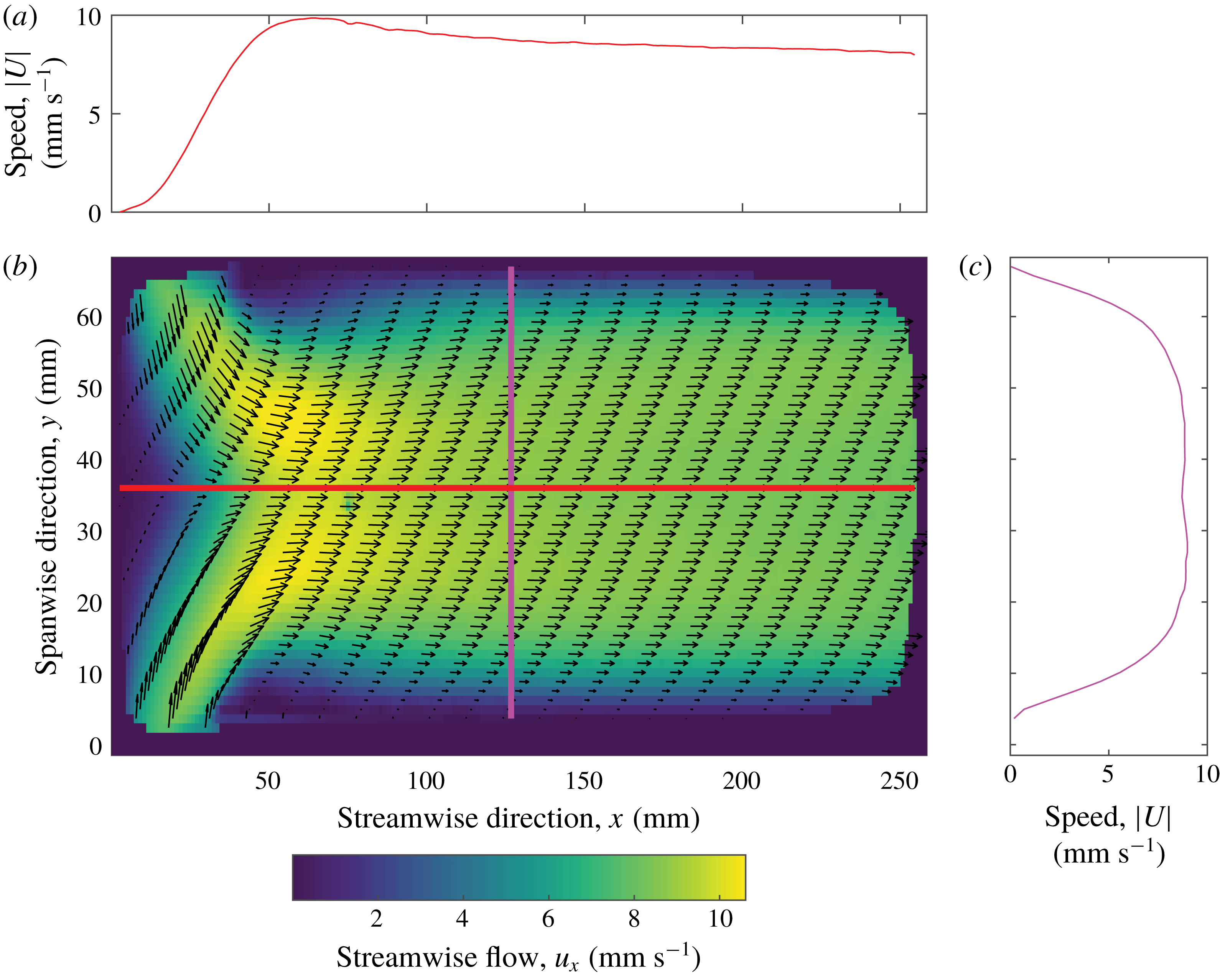
We use particle tracking velocimetry to produce velocity fields from particle motions (Ouellette, Xu & Bodenschatz Reference Ouellette, Xu and Bodenschatz2006). Then we use front tracking velocimetry to produce chemical front velocities from the concentration fields and velocity fields (Nevins & Kelley Reference Nevins and Kelley2017, Reference Nevins and Kelley2018). We varied the frame rate among experiments, from 15 Hz for slow flow to 45 Hz for fast flow, to ensure good particle tracking. Figure 17 shows an example velocity field from a single-layer experiment, and figure 18 shows an example velocity field from a two-layer experiment. Both experiments produced flows nearly uniform and unidirectional (in the
 $\hat{\boldsymbol{x}}$
direction) over most of the field of view. The two-layer experiment produced a slightly more uniform flow, partially because the magnet was better aligned during that experiment. However, uniformity is not essential since we measure both the local flow velocity and the local apparent front velocity directly. Once the current
 $J$
is switched on, two-layer experiments take longer to reach full speed than single-layer experiments because of the added inertia of the lubrication layer.
Mean flow in a single-layer experiment. Red and magenta lines indicate cross-sections where we measured the speed profiles plotted in (a) and (c), respectively.

Mean flow in a two-layer experiment. Red and magenta lines indicate cross-sections where we measured the speed profiles plotted in (a) and (c), respectively.

In our simulations the front direction was always
 $\hat{\boldsymbol{n}}=\hat{\boldsymbol{x}}$
, but in our experiments the front is not always oriented in the streamwise direction. Initially, reacted regions are typically roughly circular, so the leading edge experiences supporting flow, while the trailing edge experiences opposing flow. When a flow is not strictly one-dimensional, the speeds of front elements are affected by the component of the flow locally normal to the front,
 $\boldsymbol{u}\boldsymbol{\cdot }\hat{\boldsymbol{n}}$
. This dot product is positive for supporting flow and negative for opposing flow. Tangential front displacement has no effect, since fronts are defined only as contours of equal concentration.
6 Experimental results
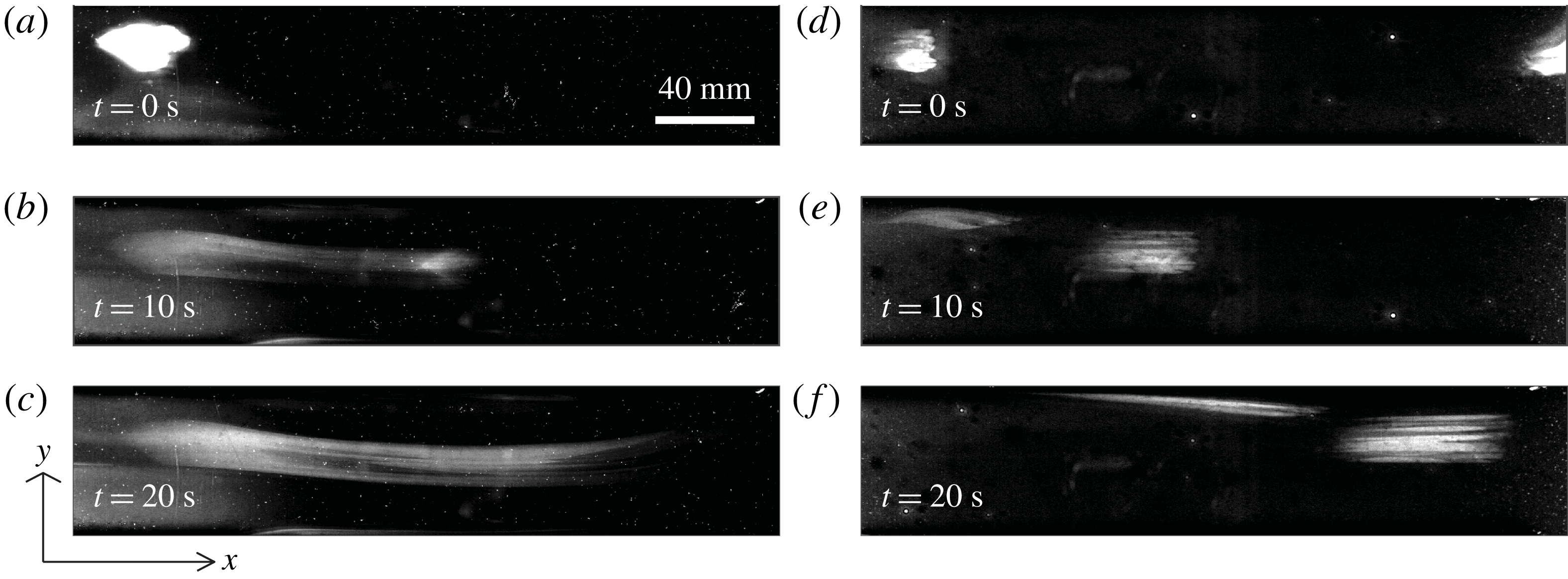
Using the apparatus described in § 5, we measured the growth of reacted regions under the influence of uniform flows with different speeds. Table 1 lists experimental parameters. Figure 19 shows a series of images from each of two experiments, one using the single-layer system, and the other using the two-layer system. (Supplemental Movie 3 shows one experiment in greater detail.) Although the flows in these two experiments have comparable speeds, the reacted regions evolve in qualitatively different ways. In the single-layer experiment shown in figure 19(a–c), the reacted region becomes smeared in the streamwise direction over time, therefore dimming. The left end of the region appears to remain nearly stationary. There, the front propagation direction
 $\hat{\boldsymbol{n}}$
points left, and the rightward flow opposes it, so our observation of a nearly stationary front implies
 $v_{a}\approx U\gg v_{0}$
. The right end of the region moves to the right with propagation direction
 $\hat{\boldsymbol{n}}$
pointing right. The rightward flow supports the front, but measurements show its speed to be slightly less than the flow speed, so
 $v_{a}<0$
. This behaviour was predicted by our simulations, as shown in figure 6(b):
 $v_{a}\approx U$
in opposing flow, and
 $v_{a}<0$
in supporting flow. Interestingly, this behaviour also leads to dilution of the reaction region, which the eikonal equation could not predict. The two-layer experiment shown in figure 19(d–f) involves much less smearing, consistent with the predictions of figure 14.
Snapshots of the BZ reaction in a single-layer experiment (a–c) and a two-layer experiment (d–f). In both experiments,
 $U\approx 13~\text{mm}~\text{s}^{-1}$
and flow goes from left to right, but the reacted regions that are initially located near the top left evolve differently. Streamwise smearing is much stronger in the single-layer system because of greater vertical shear.

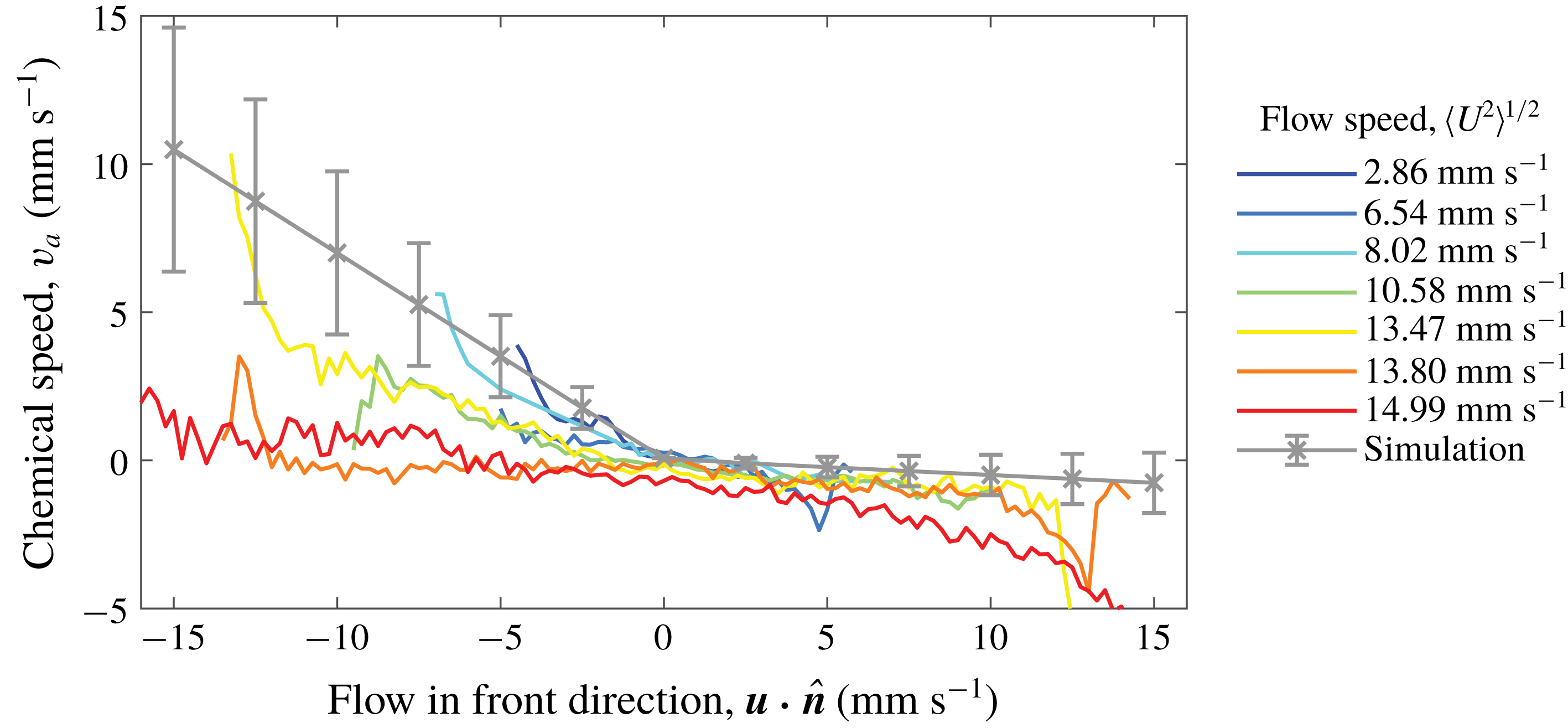
Having shown that the qualitative speeds of experimental fronts in opposing and supporting flows are consistent with trends predicted by our simulations, we now make quantitative comparisons. We used front tracking to measure chemical speeds and total speeds at many locations on all fronts in 7 single-layer experiments, each with a different flow speed
 $U$
. For each experiment, we calculated the mean apparent chemical speed,
 $v_{a}$
, at all locations with similar values of
 $\boldsymbol{u}\boldsymbol{\cdot }\hat{\boldsymbol{n}}$
(bins
 $0.25~\text{mm}~\text{s}^{-1}$
in extent, discarding bins with fewer than 100 measurements). We also calculated the mean apparent chemical speed at locations with similar values of
 $\boldsymbol{u}\boldsymbol{\cdot }\hat{\boldsymbol{n}}$
for all the simulations plotted in figure 6, combining the simulations to produce a single curve, and including error bars sized according to the variation of
 $v_{a}$
due to front smearing over the duration of the simulations. Figure 20 shows the results. Experimental measurements show similar trends to the simulation results:
 $v_{a}<0$
for supporting flows (
 $\boldsymbol{u}\boldsymbol{\cdot }\hat{\boldsymbol{n}}>0$
), and
 $v_{a}$
grows with the magnitude of opposing flows (
 $\boldsymbol{u}\boldsymbol{\cdot }\hat{\boldsymbol{n}}<0$
). Five of the seven experimental curves fall within or near the error bars of the prediction from simulations.
Variation of signed front speed with the front-normal flow speed
 $\boldsymbol{u}\boldsymbol{\cdot }\hat{\boldsymbol{n}}$
in single-layer experiments and simulations. Error bars are developed from data in figure 6. Experiments and simulations agree reasonably well.

Two of the five experimental curves in figure 20 do not fall near the prediction from simulations and deserve further attention. Both experiments involved fast flow that caused severe smearing and poor contrast, making front tracking difficult. When diluted this much, the reacted regions appear to drastically shrink everywhere. The dilution was extreme enough that no reacted region appeared again even when the drive current
 $J$
was switched off. That behaviour is qualitatively different from experiments with slower flow, in which reacted regions always began growing again. Extreme dilution preventing reaction is consistent with a blowout event due to high stretching (Nevins & Kelley Reference Nevins and Kelley2016). In this scenario the stretching is in the depth direction rather than the
 $x$
–
 $y$
plane. Shrinking and disappearance of the reacted region lowered
 $v_{a}$
. The blowout event indicates a limitation of the eikonal approximation, because in this case the magnitude of the concentration field cannot be neglected. Thus we hypothesize that this qualitative change in front behaviour occurs at a critical value of
 $Da_{I}$
, and we note that
 $Da_{I}$
is lower for the two anomalous experiments than for any others. The initial size of the reacted region may also play a secondary role.
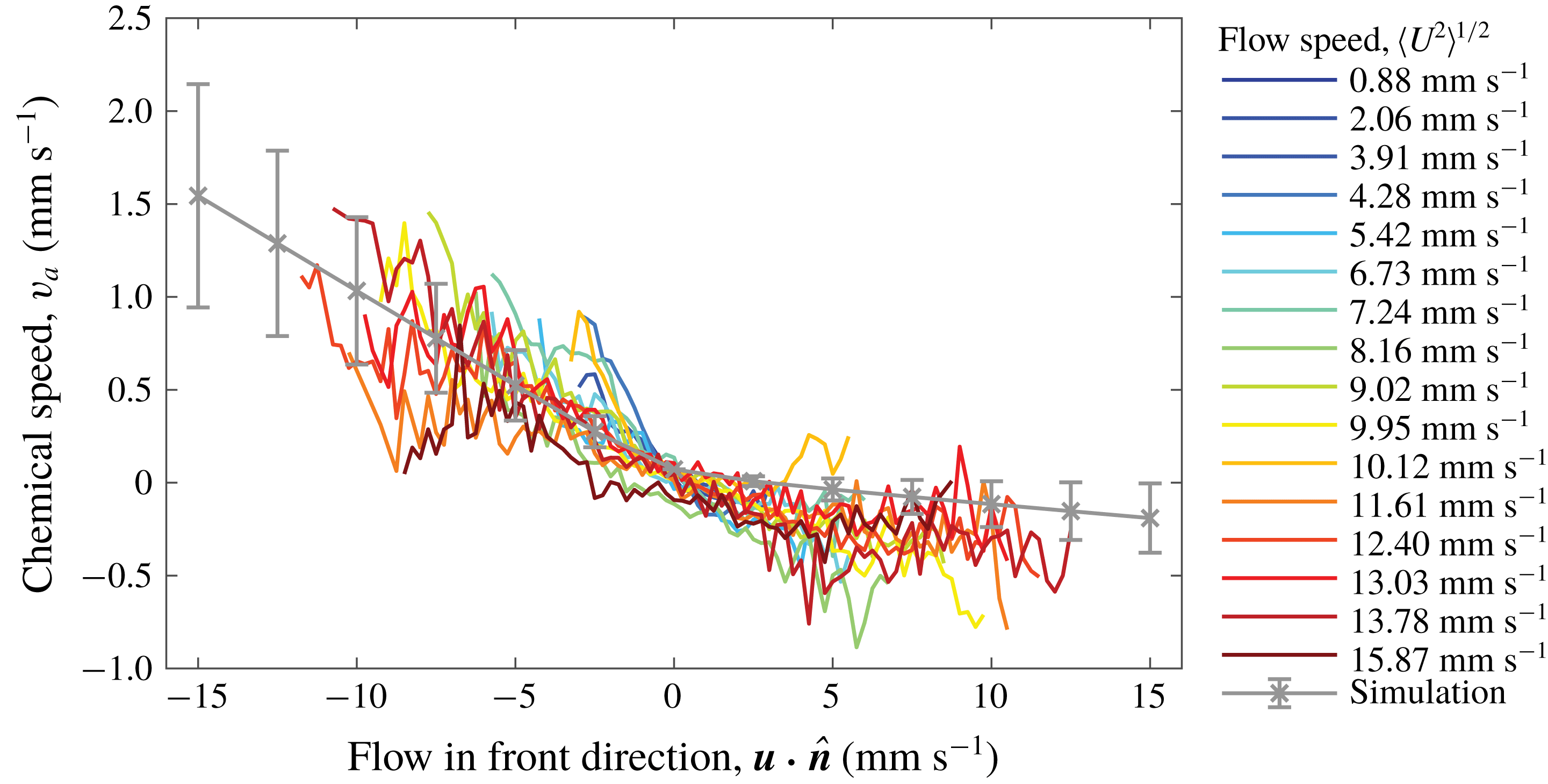
Two-layer experiments also deserve consideration. Using the same methods, we calculated the mean of
 $v_{a}$
conditioned on
 $\boldsymbol{u}\boldsymbol{\cdot }\hat{\boldsymbol{n}}$
in 16 two-layer experiments and in all the two-layer simulations plotted in figure 14. Figure 21 shows the results. All experimental curves fall within or near the error bars of the prediction from simulations. The shape of the graph is similar to single-layer experiments, but the magnitude of
 $v_{a}$
is only approximately 20 % as large, consistent with the fact that
 $\unicode[STIX]{x2202}u_{x}/\unicode[STIX]{x2202}z$
is only approximately 20 % as large in the two-layer system as in the single-layer system (figures 2 and 12). No blowout events of the sort observed in the single-layer system are apparent, although surface speeds are higher. Reduced smearing and dilution make the eikonal approximation more accurate. Blowout in a two-layer system would require much higher surface flow speeds, an additional benefit of two-layer experiments.
Variation of signed front speed with the front-normal flow speed
 $\boldsymbol{u}\boldsymbol{\cdot }\hat{\boldsymbol{n}}$
in two-layer experiments and simulations. Error bars are developed from data in figure 14. Experiments and simulations agree reasonably well.

In our experiments,
 $v_{a}$
varies with
 $\boldsymbol{u}\boldsymbol{\cdot }\hat{\boldsymbol{n}}$
in a way that is quantitatively consistent with predictions from our simple simulation built on the eikonal approximation, neglecting curvature and assuming thin fronts moving at constant speed, despite the fact that
 $Da_{I}$
was small in some cases. The match holds for single-layer and two-layer experiments.
Reaction fronts are characterized not only by a chemical speed, but also by a thickness, which is the distance separating reacted (
 $C\approx 1$
) and unreacted (
 $C\approx 0$
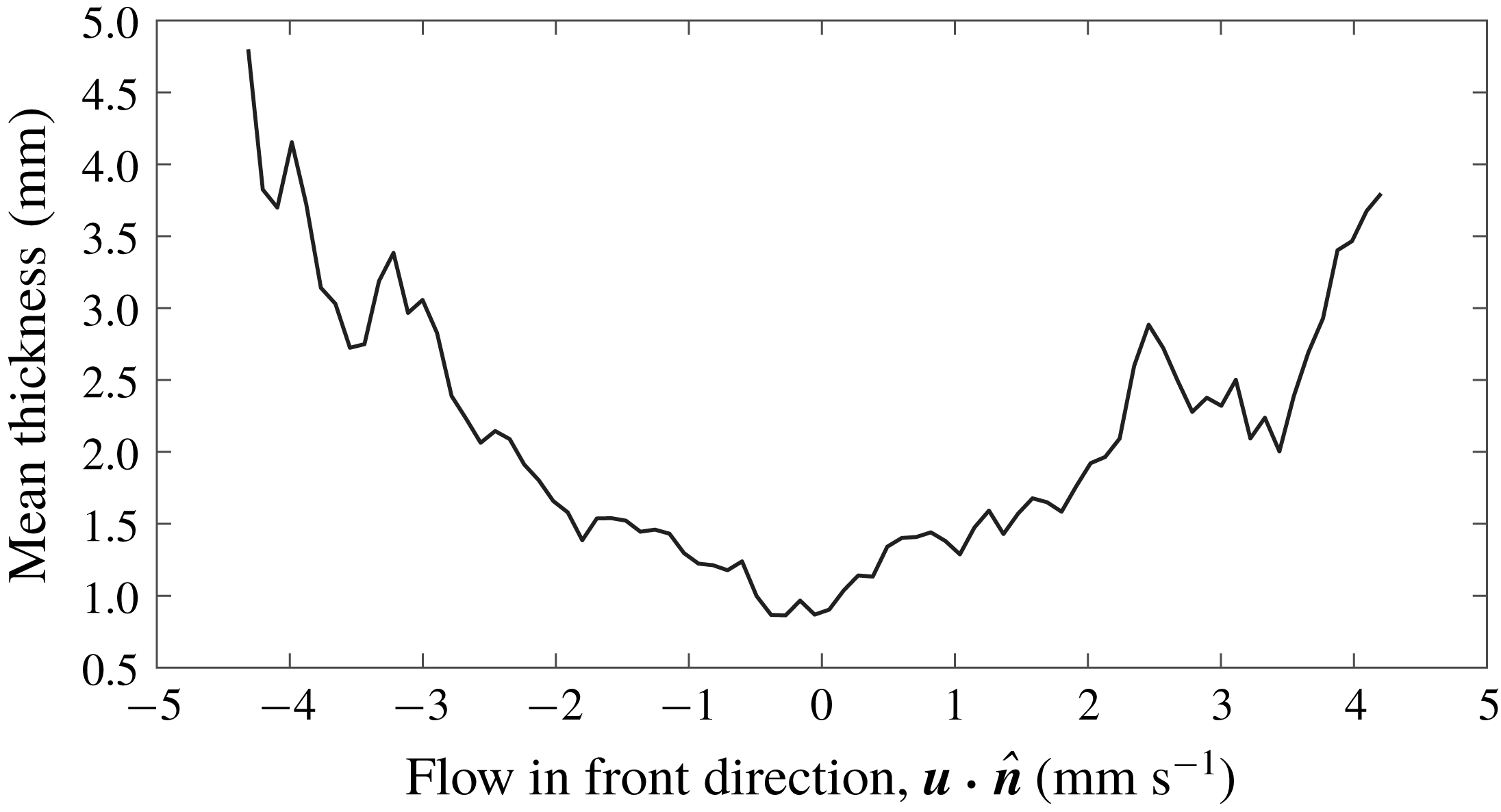
) regions, as represented by a fitting parameter (Nevins & Kelley Reference Nevins and Kelley2017). Predicting thickness is impossible with our simple simulations, which are built on the thin-front assumption. Simulations built from numerical solutions of equation (1.1) would predict front thickness but are substantially more numerically demanding and lie beyond the scope of this paper. Our experimental measurements, however, include front thickness. We calculated the mean thickness, conditioned on
 $\boldsymbol{u}\boldsymbol{\cdot }\hat{\boldsymbol{n}}$
, for all fronts in the single-layer experiment with
 $U=2.86~\text{mm}~\text{s}^{-1}$
. As shown in figure 22, fronts appear thicker when
 $\boldsymbol{u}\boldsymbol{\cdot }\hat{\boldsymbol{n}}$
has greater magnitude, whether positive or negative. Greater normal speed causes greater vertical shear, which makes fronts thicker, regardless of whether the flow supports or opposes front propagation. Future work might characterize the variation of front thickness with flow speed in more detail, perhaps providing a functional form to explain the variation shown in figure 22.
Variation of front thickness with the front-normal flow speed
 $\boldsymbol{u}\boldsymbol{\cdot }\hat{\boldsymbol{n}}$
in single-layer experiments. Vertical shear increases front thickness in either supporting or opposing flow.

7 Conclusions
In this paper we provided an explanation for the puzzling prior observation that apparent chemical speed of reaction fronts depends on flow speed in thin-layer experiments (Nevins & Kelley Reference Nevins and Kelley2018). Assuming that the fronts are sharp and that their actual chemical speed is constant, we simulated their motion in vertical cross-sections of thin-layer flows. We found that even if fronts are initially vertical, shear distorts them over time, so that locating apparent fronts using depth-averaged concentration leads to apparent chemical speeds which differ from the true chemical speed. However, simulations also showed that adding a lubrication layer can reduce shear distortion by 80 %. Single-layer experiments designed to match the simulations showed the same distortion by shear, and two-layer experiments showed the same reduction in distortion. The dependence of apparent chemical speed on flow speed agreed closely between simulation and experiment, for both single-layer and two-layer systems. The agreement held even when dimensionless parameters suggested the underlying assumptions to be unfounded. Our results resolve the puzzle by showing how the observed variation can arise from the dynamics proposed by Mitchell & Mahoney (Reference Mitchell and Mahoney2012), via shear. The agreement between simulations and experiments also further validates our front tracking algorithm (Nevins & Kelley Reference Nevins and Kelley2018) by confirming that the results it revealed are physical.
Based on our results, we recommend the immiscible two-layer configuration for reactive mixing experiments because it substantially reduces shear and produces apparent chemical speeds much closer to the true chemical speed. Whereas velocity measurements from particle tracking or particle image velocimetry are relatively unaffected by 3-D phenomena until some forcing threshold is exceeded (Kelley & Ouellette Reference Kelley and Ouellette2011; Tithof et al.
Reference Tithof, Martell and Kelley2018), apparent front speed is strongly affected by 3-D phenomena, even under gentle forcing. The effect is much more pronounced in single-layer and Hele-Shaw systems than in two-layer systems. Although we did not perform Hele-Shaw experiments, we hope our predictions from simulations will be useful to future researchers. In this work, we have considered only a single lubricant, and only a single lubrication layer thickness,
 $h_{d}=5~\text{mm}$
. Both could be optimized to reduce shear further. In particular, it is known (Suri et al.
Reference Suri, Tithof, Mitchell, Grigoriev and Schatz2014) that increasing the viscosity of the electrolyte layer greatly reduces shear. Using the two-layer configuration does introduce new technical challenges, notably that reaction bubbles are more difficult to eliminate, and stirring the solution after adding ferroin is trickier. Still, they can be managed with careful experimental methods.
Open questions remain and give opportunities for additional studies. Apparent front speed displays a piecewise-linear variation with flow speed in both the uniform flows considered here and the vortex flows considered in Nevins & Kelley (Reference Nevins and Kelley2018) – but the slopes differ. Explaining that difference would be an interesting topic for future work. The non-uniformity of vortex flow may provide the answer, since the local vertical shear depends on the local speed and direction. Initial studies might use Kolmogorov-like flows with simple horizontal speed variation, and correspondingly simple variation of vertical shear. Rotation may have separate effects and could be considered later. Time-dependent flows may involve still more complications.
In future work, it would be interesting to check the agreement between experiments and simulated front dynamics when the Damköhler numbers are even lower than considered here, to find the limits of validity of the eikonal approximation. One likely limitation is visible in figure 20, where dilution of the front led to extinction. Since the eikonal equation does not consider the concentration on either side of the front, and extinction depends on local concentration, extinction cannot be predicted using the eikonal equation. Put another way, because a no-slip boundary lies at the bottom of the single layer, the disappearance of the front cannot be attributed to the front being blown downstream, since there is always a slow zone, where
 $u_{x}<v_{0}$
. The front transitions from a pinned state to an unreacted state, without being advected away. Since this effect appears in the single-layer configuration but not the two-layer configuration, depth shear is the probable cause. We have also observed extinction of this kind in vortex and bluff body flow (Nevins & Kelley Reference Nevins and Kelley2016; Wang et al.
Reference Wang, Tithof, Nevins, Colón and Kelley2017). The eikonal equation as stated above is also unable to explain the frozen fronts observed previously (Atis et al.
Reference Atis, Saha, Auradou, Salin and Talon2013). The eventual detaching from a no-slip location may be due to front stretching or the effects of curvature, which are both beyond the simple eikonal equation we have used, and could be considered in future work.
Finally, we have considered only the Belousov–Zhabotinsky reaction, which has
 $v_{0}=72~\unicode[STIX]{x03BC}\text{m}~\text{s}^{-1}$
. Future work might test that our predictions hold for different chemical kinetics and different true chemical speeds.
Acknowledgements
The authors are grateful for experimental design help from R. S. Russell, J. Wang and J. Tithof, and for editing assistance on an earlier draft of this manuscript from J. Thomas. T.D.N. was supported by the Department of Defense through the National Defense Science and Engineering Graduate Fellowship (NDSEG) programme.
Supplementary movies
Supplementary movies are available at https://doi.org/10.1017/jfm.2019.460.