





1. Introduction
Surface gravity waves in coastal and estuarine environments commonly propagate in the presence of ambient currents that vary horizontally and vertically. This situation is especially relevant near tidal inlets and river mouths, where the flow is strongly affected by boundary-layer processes and bathymetric control, leading to velocity profiles with pronounced vertical shear and, in general, non-trivial vorticity distributions. When waves propagate over a gently sloping bed while encountering such currents, their evolution reflects the combined action of shoaling, Doppler shifting and shear-induced modifications of dispersion and momentum–energy exchanges. Under sufficiently strong opposing currents the interaction can become intense, with rapid steepening, enhanced dissipation and ultimately wave blocking, in which wave energy is unable to propagate upstream. Strictly, wave blocking is a group-velocity (energy-flux) condition. However, in strongly sheared and near-breaking regimes, phase speed remains the most reliably measurable kinematic quantity and a necessary intermediate step to constrain dispersion and, ultimately, energy-transport estimates.
A detailed understanding of wave–current interactions is required in various circumstances, such as in lagoon inlets, where diurnal flood and ebb tidal flows follow or propagate against incident wave trains (see, e.g. Chiapponi et al. Reference Chiapponi, Palmisani, De Piccoli, Matticchio and Longo2015). A recent study by Brocchini et al. (Reference Brocchini, Marini and Baldoni2026) provides a comprehensive investigation of wave–current interactions at microtidal river mouths. The analysis, which integrates long-term in situ observations with numerical modelling for the Misa River (Italy), demonstrates that opposing fluvial discharges substantially modify incident sea waves and, consequently, enhance fluvial flood hazards and induce significant morphological adjustments of the river mouth system.
From a theoretical standpoint, a rigorous linear formulation of surface gravity waves propagating on vertically sheared (depth-dependent) currents yields an eigenvalue problem for the wave-induced vertical velocity. This problem is conventionally expressed in terms of the Rayleigh equation, which is mathematically equivalent to the inviscid Orr–Sommerfeld equation subject to free-surface boundary conditions (Peregrine Reference Peregrine1976; Shrira Reference Shrira1993). Except for special current profiles, analytical progress is limited and historically a variety of idealisations have been explored. Early contributions derived dispersion relations by approximating realistic profiles with piecewise-linear segments (Thompson Reference Thompson1949; Biesel Reference Biesel1950) or by adopting simple functional forms such as exponential shear (Abdullah Reference Abdullah1949). For long waves on general currents, compact integral expressions were obtained by Burns (Reference Burns1953). Further developments included dispersion relations and velocity fields for bilinear profiles and numerical strategies for more general current distributions (Dalrymple Reference Dalrymple1974), together with studies illustrating how vorticity modifies wave properties and surface elevation (Fredsøe Reference Fredsøe1974; Dalrymple & Cox Reference Dalrymple and Cox1976). A broad synthesis of wave–current interaction mechanisms, covering uniform, slowly varying and depth-dependent currents, remains the classical review by Peregrine (Reference Peregrine1976).
A major step toward practical modelling of waves on vertically sheared currents was the development of approximate dispersion relations based on weak-shear expansions. The primary finite-depth first-order approximation for a current consisting of an arbitrary depth-uniform component and a weak vertically varying component was introduced by Skop (Reference Skop1987), while Kirby & Chen (Reference Kirby and Chen1989) derived the corresponding second-order correction for vertically sheared flows. Subsequent analyses clarified the range of applicability of this class of approximations. In particular, Banihashemi & Kirby (Reference Banihashemi and Kirby2019) showed that the framework of Skop (Reference Skop1987) and Kirby & Chen (Reference Kirby and Chen1989) remains valid when the depth-uniform component of the current is of order one relative to the wave phase speed, provided that the vertically varying part remains weak. Related extensions to currents of arbitrary direction were discussed by Ellingsen & Li (Reference Ellingsen and Li2017). They also derived an approximate dispersion relation for currents whose magnitude and direction may vary arbitrarily with depth, clarifying the conditions of applicability and showing improved robustness in cases where the classical approximation may fail; a second-order correction was also provided. Alongside such closed-form approximations, accurate numerical procedures are now available for computing dispersion curves on arbitrary shear flows by solving the Rayleigh problem efficiently; in particular, Maxwell & Ellingsen (Reference Maxwell and Ellingsen2020) developed continuation (path-following) methods that exploit the analyticity of the dispersion relation to compute large sets of dispersion data points at low computational cost.
For slowly varying environments, the evolution of wave amplitude and energy transport is often framed in terms of wave rays and conservation of wave action (Bretherton & Garrett Reference Bretherton and Garrett1968). For linear waves propagating on arbitrarily vertically sheared currents, the corresponding general conservation law was derived by Voronovich (Reference Voronovich1976), extending the classical wave-action framework to the case in which the wave field is governed by the eigenfunctions of the Rayleigh problem. Addressing the need for formulations suitable for practical wave modelling, Quinn et al. (Reference Quinn, Toledo and Shrira2017) derived an explicit wave-action conservation equation for horizontally inhomogeneous vertically sheared currents, based on an approximate treatment of the Rayleigh problem. Subsequent developments refined the weak-shear approximation. In particular, Banihashemi et al. (Reference Banihashemi, Kirby and Dong2017) derived a corrected expression for the current contribution to the group velocity, while Banihashemi & Kirby (Reference Banihashemi and Kirby2019) obtained asymptotic expressions for wave-action density and flux, and showed that their predicted action flux is more accurate than that obtained from the formulation of Quinn et al. (Reference Quinn, Toledo and Shrira2017) in benchmark cases. These theoretical developments are particularly relevant to coastal settings where waves shoal over mild slopes while interacting with currents whose vertical structure departs markedly from depth-uniform assumptions.
Wave blocking represents a particularly strong regime of wave–current interaction. Laboratory experiments have long indicated that, under steady conditions, the dominant kinematic influence of a current may be interpreted as a Doppler shift, and that after Doppler correction the wave kinematics can remain close to linear-theory expectations over a broad range of conditions, including cases with breaking (Lai et al. Reference Lai, Long and Huang1989). For the idealised case of constant vertical shear, explicit blocking conditions have been analysed by Maïssa et al. (Reference Maïssa, Rousseaux and Stepanyants2016), who showed how vorticity modifies the blocking threshold relative to the depth-uniform-current case. Within the weak-shear approximation framework, Banihashemi et al. (Reference Banihashemi, Kirby and Dong2017) further compared approximate blocking predictions with full numerical results for constant shear and identified regimes in which the approximate theory breaks down.
Focusing on this regime, Chawla & Kirby (Reference Chawla and Kirby2002) investigated current-limited breaking in monochromatic and random waves at blocking points. In the monochromatic-wave experiments, nonlinear modulation generated higher-frequency components as Benjamin–Feir sidebands, which were then selectively blocked by the opposing current, producing a spectral downshift; dissipation models were also proposed. Later, Yao & Wu (Reference Yao and Wu2004) examined energy dissipation in unsteady deep-water breaking wave groups on following and opposing currents, including partial-blocking conditions, highlighting how strong opposing currents can substantially alter spectral properties and energy-flux losses. Spatially varying opposing currents introduce additional complexity, and Ma et al. (Reference Ma, Dong, Perlin, Ma, Wang and Xu2010) further documented nonlinear modulation, sideband evolution and frequency downshift, even for small initial steepness. They also emphasised that gradual blocking can disrupt wave-action conservation downstream and accelerate spectral changes.
Complementing laboratory studies, high-resolution numerical simulations based on Reynolds-averaged Navier–Stokes–volume-of-fluid frameworks have clarified specific features of current-induced breaking and blocking, including reductions in limiting steepness and the coupled response of mean water level through the interplay of radiation stress and current-induced surface tilting (Chen & Zou Reference Chen and Zou2018). An additional perspective on blocking is provided by the analogy between counter-current-induced blocking points and horizon-like behaviour in wave propagation (Nardin et al. Reference Nardin, Rousseaux and Coullet2009).
From an experimental perspective, the pioneering laboratory investigations conducted by Kemp & Simons (Reference Kemp and Simons1982, Reference Kemp and Simons1983) yielded fundamental quantitative data on wave–current interactions in turbulent channel flows. These studies documented the modification of mean velocity profiles, turbulence characteristics, bed shear stress, free-surface elevation and wave attenuation for waves propagating both in the direction of and opposing a background current. However, systematic experimental validation encompassing a broad range of prescribed vertical profiles is still largely lacking. A significant experimental contribution was presented by Suastika (Reference Suastika2004), who conducted an extensive laboratory study of wave blocking under systematically intensified opposing currents. The investigation reported pronounced wave shortening, steepening, breaking, reflection and associated spectral transformations in the vicinity of blocking conditions, thereby underscoring the critical roles of energy dissipation and wave reflection processes. Although the study primarily addressed the phenomenological characterisation and modelling of wave blocking, the acquisition of detailed measurements of prescribed vertical current profiles and their impact on phase-velocity predictions did not constitute its principal objective.
Building on previous laboratory work, the present study examines a complementary facet of the problem: the deliberate control of the vertical structure of the opposing current using flow conditioners (FCs). This approach makes it possible to generate repeatable shear profiles that can be isolated and compared under otherwise comparable wave conditions. A second, closely related limitation is that only a small number of laboratory investigations report simultaneous, spatially resolved measurements of the subsurface velocity field under such strong interaction regimes, even though these measurements are crucial for quantifying momentum and energy budgets beyond what can be deduced from free-surface data alone.
For these reasons, we performed controlled flume experiments of regular waves propagating over a gently sloping bed against a steady counter-current whose vertical profile is deliberately shaped to span a range of shear structures. Using interchangeable flow-conditioning elements, we generate distinct velocity distributions (near-surface-intensified, near-bottom-intensified and more strongly curved profiles, in addition to the profile that emerges naturally in the absence of external control) at comparable bulk current strengths. Free-surface elevations are recorded along the flume, whereas particle image velocimetry (PIV) provides time-resolved velocity fields in the region of the strongest interaction.
To the authors’ knowledge, few laboratory studies combine deliberately prescribed vertical shear profiles with collocated free-surface and PIV measurements under near-blocking conditions. The resulting data set enables robust and independent estimates of phase velocity from both surface and subsurface signals, and supports a targeted assessment of modelling assumptions by comparing observations with the uniform-current approximation, shear-aware approximate dispersion relations (Kirby & Chen Reference Kirby and Chen1989; Ellingsen & Li Reference Ellingsen and Li2017) and numerical solutions of the Rayleigh problem (Maxwell & Ellingsen Reference Maxwell and Ellingsen2020). The present analysis does not derive a new dispersion relation that incorporates vertical shear. Rather, it evaluates existing shear-aware formulations against controlled experimental observations.
The paper is organised as follows. Section 2 reports the theoretical and numerical models adopted for the phase-velocity estimates, while § 3 describes the experimental facility, the controlled current profiles and the measurement and data-processing procedures.
Section 4 presents and compares the phase-velocity estimates obtained from the approximate models, the full numerical Rayleigh solution and the experimental measurements.
Finally, § 5 brings together the main findings and discusses their implications for wave–current interaction in strongly sheared flows over mildly sloping bathymetry.
2. Phase velocity
A rigorous determination of the phase velocity associated with a generic current profile requires the formulation and solution of an appropriate eigenvalue problem.
We consider a linear monochromatic surface gravity wave propagating in the streamwise direction over a horizontally uniform, vertically sheared current profile. In the framework of linear inviscid theory, the wave induces pressure and velocity perturbations superimposed on the background current, and the resulting flow is governed by the Euler equations. This equation can be traced back to the following boundary-value problem for vertical velocity
 $v(z)$
in the hypothesis of collinearity between current and waves (see, e.g. Shrira Reference Shrira1993 and Ellingsen & Li Reference Ellingsen and Li2017 for details)
 \begin{equation} \left \{ \begin{array}{ll} v''(z)-k^2v(z)=\dfrac {U''(z)}{U(z)-c}v(z)\quad \text{for }z\in [-h,0],\\[12pt] \left (U_0-c\right )^2v'(0)-\left [U'_0\left (U_0-c\right )+g\right ]v(0)=0,\\[12pt] v(-h)=0, \end{array}\right . \end{equation}
known as the Rayleigh problem, where
 $U(z)$
is the horizontal current profile,
 $c=\omega /k$
is the phase velocity,
 $U_0=U(0)$
,
 $U'_0=U'(0)$
and the prime indicates the differentiation;
 $\omega$
is the angular frequency,
 $k$
is the wavenumber,
 $h$
is the local water depth and
 $g$
is the gravitational acceleration. Equation (2.1) admits an analytical solution for a uniform current, resulting in the following dispersion relation, widely discussed in Peregrine (Reference Peregrine1976):
 \begin{equation} (\overline {U}-c)^2=c_0^2,\quad c_0=\sqrt {\dfrac {g}{k}\tanh (kh)}, \end{equation}
where
 $\overline {U}$
is the uniform current and
 $c_0$
is the linear phase velocity in still water (i.e. in the absence of a current). In all other cases, a numerical solution or approximate solutions are required, such as those presented in Kirby & Chen (Reference Kirby and Chen1989) and Ellingsen & Li (Reference Ellingsen and Li2017), to name a few. In particular, a first-order correction by Ellingsen & Li (Reference Ellingsen and Li2017) reads
 \begin{equation} \left \{ \begin{array}{ll} c-U_0=c_0\left [\sqrt {1+\delta (k)^2}-\delta (k)\right ],\\[12pt] \delta (k)=\dfrac {1}{c_0\sinh (2kh)}\displaystyle \int _{-h}^0U'(z)\sinh [2k(z+h)]\,\text{d}z, \end{array}\right . \end{equation}
where
 $\delta (k)$
is a dimensionless depth-averaged shear, equal to 0 for a uniform-current profile. A second-order correction (Ellingsen & Li Reference Ellingsen and Li2017) derives from the solution of the following equation:
 \begin{equation} (c-U_0)^2+2(c-U_0)c_0\delta (k)+c_0^2[\Delta (k)-1]=0, \end{equation}
where
 $\Delta (k)$
contains the effects of the curvature and is equal to
 \begin{equation} \left \{ \begin{array}{ll} \Delta (k)=-\dfrac {2(c-U_0)}{kc_0^2\sinh (kh)}\displaystyle \int _{-h}^0\dfrac {U''(z)}{U(z)-c}\sinh [k(z+h)]\sinh (kz)[\tilde {U}-\tilde {u}(z)]\,\text{d}z,\\[12pt] \tilde {u}(z)=-\dfrac {2k\sinh (kh)}{\sinh (2kh)\sinh (kz)}\displaystyle \int _{z}^0U(\zeta )\cosh [k(2\zeta +h-z)]\,\text{d}\zeta ,\\[12pt] \tilde {U}=\tilde {u}(-h). \end{array}\right . \end{equation}
The parameter
 $\Delta (k)$
approaches zero in the case of a linearly varying current profile.
Alongside the approximations of the dispersion relation, it is possible to work directly on the numerical solution of the eigenvalue problem (2.1), defined as a ‘full numerical solution’. In this case, the implementation of a shooting method was found to be an effective approach, imposing two boundary conditions at
 $z=0$
in parametric form as follows:
 $[U'_0(U_0-c) + g]v(0)=b$
and
 $(U_0-c)^2v'(0)=b$
, where
 $b$
is the parameter. This approach involved the selection of an arbitrary value for the parameter
 $b$
and the subsequent determination of the value of
 $k$
that satisfies the boundary condition
 $v(-h)=0$
. The result is independent of the value of
 $b$
. Upon determining the value of the full numerical wavenumber
 $k=k_{fn}$
, the phase velocity is calculated as
 $\omega /k_{fn}$
.
Equations (2.1)–(2.5) are used here as local linear dispersion models. The measured current profile and the local water depth in the PIV region are supplied to the models, whereas the gradual streamwise variation of the water depth is neglected within the local calculation. This approximation is supported by the limited streamwise extent of the PIV field of view and by the mild local bottom slope. The models are therefore expected to capture the leading Doppler- and shear-induced modifications of the phase velocity, but they do not include finite-amplitude corrections, crest–trough asymmetry, harmonic generation, wave breaking or the non-local evolution associated with shoaling. Consequently, their comparison with the measurements should be interpreted primarily as a relative assessment of alternative representations of the current profile, rather than as a complete nonlinear prediction of the absolute phase velocity.
3. The experiments
The experiments were conducted in a recirculating hydraulic flume specifically designed for controlled investigations of wave–current interactions, located at the Hydraulics Laboratory of the University of Parma. The flume reproduces free-surface flows under prescribed boundary conditions and provides adequate length for flow development and the installation of measurement devices.
The flume is 10 m long, 0.3 m wide and has glass vertical sidewalls that are 0.47 m high. A recirculating system delivers and reuses water to enable continuous operation with a maximum flow rate of 30 l s−1, while a slope-adjustment device allows the bed inclination to be varied. For these tests, the primary bed slope was set to 1 : 74; however, this effectively changed to 1 : 47 in the PIV measurements section due to the installation of a false bottom necessary to install a 45
 $^\circ$
mirror to transform the horizontal laser sheet to a vertical laser sheet, since the iron bottom of the flume was not transparent. Smooth transition sections were installed at the entrance and outlet to moderate the inflow and outflow and minimise turbulence and flow separation at the boundaries. On the opposite side of the current flow entrance, a plunger-type wavemaker was installed. The wave generation system allows for the generation of sinusoidal monochromatic waves with a period in the range
 $0.5\,\text{s}\lt T\lt 2\,\text{s}$
and a wave height of up to 10 cm.
The measurements span the entire length of the flume, accommodating distributed and point-based observations. Twelve resistive level probes with an accuracy of 0.5 mm were placed at multiple stations to record elevations of the free surface at a data rate of 100 Hz, while PIV measurements were conducted near the current inlet, i.e. in the region where the opposing current enters the flume and where the wave–current interaction is most pronounced. The flow rate was measured with a magnetic flow meter with an accuracy of 0.5 %. To ensure smooth entry conditions and minimise large-scale turbulence, a flow-straightening device was installed at the inlet. Consisting of an array of tightly packed small-diameter pipes, this device effectively distributes the incoming jet and promotes a nearly uniform velocity profile at the channel entrance. Figure 1 shows a schematic diagram of the complete set-up.
A PIV system provided by Optolution GmbH was implemented for velocity measurements close to the current entrance section. The system consisted of three elements: a laser, a camera and a synchroniser. The laser was a diode module with a power of 40 W, a wavelength of
 $450\pm 20\,\text{nm}$
and LS-Optics to spread the coherent pointwise light on a sheet used for PIV measurements. The camera was an OPTRONIS Cyclone-25-150-M with resolution
 $5120 \times 5120\,\text{px}$
, an active sensor of size
 $12.8\,\mathrm{mm}\times 12.8\,\mathrm{mm}$
, a data rate of up to 1029 fps (150 Hz at full resolution) and a CoaXPress V2.0 Interface with download capacity of
 $4 \times 12\,\rm{Gb\,s}^{-1}$
. The synchroniser was necessary for synchronising the camera exposure with laser pulses. It was attached to the laser module and communicated with the PC through a wireless serial link. Full control of the PIV system was achieved through the PIVlab MATLAB toolbox, which has been specifically developed for PIV applications (Thielicke & Stamhuis Reference Thielicke and Stamhuis2014; Thielicke & Sonntag Reference Thielicke and Sonntag2021). The PIV measurements were made in a single downstream section, at a distance of 825.5 cm (mid section) from the plunger with a field of view (FOV) of approximately
 $250\times 250\,\textrm {mm}^2$
in the mid section of the flume and a data rate of 75 pairs of frames per second, acquiring approximately 500 pairs of frames for each run. With the present FOV, the final resolution resulted in
 $49\,\unicode {x03BC}\text{m\,pixel}$
−1. The fluid was seeded with neutrally buoyant tracer particles (hollow glass spheres) of nominal mean diameter of
 $55\,\unicode {x03BC}\text{m}$
. A rough estimation of the particle relaxation time gives
 $\tau _p=\mathcal{O}(10^{-1}\,\text{ms})$
, while the Kolmogorov time scale for waves and counter-current typical of the present activity can be evaluated as
 $\tau _{\eta }=\mathcal{O}(10\,\text{ms})$
, yielding a Stokes number
 $St=\tau _p/\tau _\eta \ll 1$
, i.e. a velocity uncertainty less than 1 % (Raffel et al. Reference Raffel, Willert, Scarano, Kähler, Wereley and Kompenhans2018). A triple decomposition of the velocity field results in the separation of the current, wave and turbulent contributions (see § 3.1.2). The velocity components of the oscillatory motion are denoted by
 $u$
and
 $v$
, while
 $U$
and
 $V$
represent the mean current components and
 $u'$
and
 $v'$
denote the fluctuating contributions. These components are aligned with the horizontal
 $x$
-axis and the vertical
 $z$
-axis, respectively, according to the reference frame illustrated in figure 1.
The experimental flume and schematic of the wave probes and of the PIV camera. (a) Side view of the flume, (b) top view. Typical velocity profiles (not to scale) with (c) no FC (FC0), (d) FC1, (e) FC2 and (f) FC3. Here, s.w.l. is the still water level.

The present activity aims at characterising the wave–counter-current interaction due to different current shear and velocity profile curvature. In-house designed passive devices named ‘flow conditioners’, consisting of a package of six thin, stainless steel flat plates measuring
 $295\times 215\,\mathrm{mm^2}$
, were deployed in the wave–current flume for the experimental activity. These were positioned parallel to the bottom and spaced according to the desired horizontal velocity profile. Their role was to shape the velocity distribution of the incoming current before the PIV measurement zone. This enabled the reproduction of the following vertical velocity profiles: bottom slowed (FC1, with a spacing of 0.6 cm starting from the bottom and ending at 4.5 cm); top slowed (FC3, with a spacing of 0.6 cm starting from 6.5 cm above the bottom); and cubic (FC2, with spacings of 0.2, 0.6, 1.1, 1.8, 2.8 and 3.8 cm starting from the bottom). The tests were also conducted without the FC, which is hereinafter referred to as FC0. See figure 1(c–f).
Parameters of the experimental tests. Here,
 $T$
denotes the period of the regular waves,
 $\overline {U}$
represents the mean current velocity in the mid-section of the PIV FOV and
 $c_{lwo}$
corresponds to the local linear wave phase velocity in that section under the hypothetical condition that only waves are present.

Table 1. Long description
The table presents parameters of experimental tests involving wave and counter-current interactions. It is divided into four sections: Wave + Counter-current, Only wave, Only current, and Repeated runs. Each section lists the period of regular waves (T in seconds), mean current velocity (U with units of meters per second), flow conditioner types, and the number of tests conducted. The Wave + Counter-current section includes rows for different wave periods (1.23 s, 1.00 s, 0.87 s) and flow conditioners (0-1-2-3), with 33 to 37 tests each. The Only wave section lists one test for each wave period. The Only current section details tests for different current velocities (-0.25, -0.35, -0.48 m/s) with flow conditioners (0-1-2-3), each conducted 4 times. The Repeated runs section includes 10 tests for a wave period of 1.23 s with flow conditioner 0.
The FCs are designed to generate prescribed vertical velocity profiles that act as kinematic analogues of river-mouth-like currents while deliberately isolating the role of velocity shear from buoyancy effects. In particular, we consider two limiting classes of profiles at comparable bulk current strength: (i) near-surface-intensified currents (FC1), and (ii) near-bottom-intensified currents (FC3). These cases characterise the range of vertical shear structures often encountered in inlets and river mouths and provide a controlled basis to test the sensitivity of wave kinematics to the distribution and curvature of shear. The FC1 case produces a near-surface-intensified profile. In the field, such a structure is commonly associated with buoyant river outflows in which relatively fresh (less dense) water overlies denser saline water, potentially forming a saline wedge; in this configuration, enhanced resistance may arise from entrainment processes and strong shear at the density interface. In contrast, FC3 generates a bottom-intensified profile. Field situations that motivate this choice include flows in which the dominant resistance is exerted in the upper layers – for instance, turbid (muddy) water, or colder water entering clearer or warmer water, as well as cases in which the near-surface current is reduced by opposing wind stress, wave-breaking-induced turbulence or additional surface-layer resistance associated with surface roughness (e.g. floating debris/vegetation or ice). Under such conditions, the maximum velocity can shift downward. The FC0 case corresponds to a reference condition with a comparatively smoother distribution, representative of cases in which no marked vertical differentiation of water properties is present and the case FC2 provides a more strongly curved profile to probe sensitivity to shear curvature and to further assess the robustness of the modelling approaches to departures from simple monotonic shear. We stress that these configurations reproduce the velocity-structure effect only: the experiments are conducted in a homogeneous fluid and, therefore, do not model density stratification or the salinity-driven interfacial dynamics; rather, the above field scenarios are invoked solely as qualitative motivation for the prescribed shapes of
 $U(z)$
.
The experimental protocol involved cleaning the wires and calibrating the level probes daily, with intermediate or final calibration verifications randomly carried out during the day to ensure consistency of the calibration procedure. Then, tests were performed at increasing flow rates in steps, with the same regular wave period. After the flow rate was increased, sufficient time was allowed to ensure that a steady state was reached. Levels were acquired for 300 s and PIV images were taken until 500 pairs of frames were obtained. Without changing the FC, the wave period was then changed until the series was complete. This process was repeated for each of the four FCs. Some tests were run multiple times to verify the repeatability of the results. Finally, velocities and levels were acquired for waves alone (without current) and for current alone (without waves), with different flow rate values. For waves alone, the tests were performed without a FC.
Table 1 presents the main experimental parameters. Since more than one hundred individual tests were performed for different combinations of wave period, current intensity and FC configurations, they are presented as a compact summary of the explored parameter ranges. The mean current
 $\overline {U}$
, averaged from the horizontal velocity profile, and the local (within the FOV of the PIV system) linear wave phase speed
 $c_{lwo}$
, evaluated using
 $T$
in the linear dispersion relation without considering the current, were used to calculate the parameter
 $\overline {U}/c_{lwo}$
, which characterises the wave–current interaction. Additional information is available in Hasheminejad et al. (Reference Hasheminejad, Addona, Chiapponi and Longo2025). An example of the experimental results is reported in Supplementary Movie 1, which shows different wave–counter-current interaction conditions for
 $T=1.23\,\text{s}$
, FC0 and
 $\overline {U}/c_{lwo}$
in the range
 $-0.55$
–0. The movie shows how the velocity field changes in the presence of a shear counter-current, up to the wave blocking that is theoretically reached for
 $\overline {U}/c_{lwo}=-0.43$
and experimentally inferred, on the basis of strong attenuation and loss of a coherent propagating-wave signature, for the condition
 $U/c_{lwo}=-0.55$
.
3.1. Data analysis
3.1.1. Free-surface levels
The level measurements were analysed to extract the characteristic parameters of the waves in the sections of interest. Conventional zero-crossing analysis was used to evaluate the root mean square wave height
 $H_{rms}$
, which provides a measure of the spatial variability and attenuation of the wave field under the different wave–current configurations.
Experimental values of
 $H_{{rms}}$
measured at different cross-sections. (a) The data refer to waves with a period
 $T = 0.87\,\text{s}$
propagating against a counter-current of increasing velocity, starting from quiescent conditions (zero current), with FC1 installed. (b) The data refer to waves with a period
 $T = 1.23\,\text{s}$
propagating against a counter-current of increasing velocity, starting from quiescent conditions (zero current), with FC3 installed. The hatched yellow region indicates the experimentally inferred blocking or near-blocking region, identified from strong wave attenuation and loss of a coherent propagating-wave signature.

In the present study, the term ‘blocking’ is used in an operational sense when referring to the experimental observations. Strictly, wave blocking is a group-velocity, or energy-flux, condition. However, the present measurements do not provide streamwise-resolved current profiles over the entire flume and therefore do not allow the exact theoretical blocking point to be determined along the channel. Blocking or near-blocking conditions are therefore inferred from the combined evidence of strong spatial attenuation of the free-surface signal, loss of a coherent propagating-wave signature between adjacent probes and failure of the cross-correlation procedure to return a robust phase delay. Accordingly, the hatched regions in figure 2 should be interpreted as experimentally inferred blocking or near-blocking regions, rather than as exact theoretical blocking points.
The average phase velocity was calculated between two consecutive probes by cross-correlating the free-surface elevation signals and estimating the delay associated with the peak of the cross-correlation function. For the strongest opposing-current conditions, corresponding to blocking or near-blocking regimes, no phase-velocity estimates based on free-surface elevation measurements are reported. Under these circumstances, although a finite local phase velocity may still be present, wave-energy transmission is strongly reduced as the group velocity approaches zero. As a result, the free-surface signal no longer exhibits a sufficiently pronounced propagating-wave signature between adjacent probes, and the associated cross-correlation functions fail to present a clearly defined peak from which a reliable time delay, and therefore a robust phase-velocity estimate, can be determined.
With regard to wave reflection, in the wave-only experiments it was passively mitigated by installing a parabolic beach composed of sponge material. In the combined wave–current experiments, reflection was quantified and consistently found to remain below 10 %, with the exception of some configurations with reduced counter-current velocity. It should be emphasised that active absorption systems capable of fully suppressing reflection in non-classical flow conditions, i.e. when the flow field is not characterised solely by a simple return current, are not yet available. In this framework, the anti-reflective influence of the current becomes increasingly pronounced as the magnitude of the opposing-current velocity increases.
Figure 2 shows the spatial evolution of
 $H_{rms}$
at several cross-sections for increasing values of the non-dimensional parameter
 $|\overline {U}/c_{lwo}|$
and for two distinct flow configurations. Figure 2(a) corresponds to experiments conducted with a wave period
 $T = 0.87\,\text{s}$
and FC1. With the exception of the wave-only reference case, in which the observed reduction in wave height is primarily attributable to wave breaking, a pronounced attenuation of the wave field is observed near the current inlet. This configuration, characterised by the shortest wave period and by a current profile with a strongly developed near-surface core, is the most prone to blocking-like behaviour. In the last probe section, conditions close to blocking are observed for
 $\overline {U}/c_{lwo} = -0.31$
, while stronger attenuation and loss of a coherent propagating signature occur for
 $\overline {U}/c_{lwo} = -0.34$
and for larger absolute values of this ratio, with the inferred blocking or near-blocking region extending farther offshore.
Figure 2(b) corresponds to experiments with a wave period
 $T = 1.23\,\text{s}$
and FC3. In this case, only the highest opposing-current velocities produce substantial wave attenuation. This configuration, characterised by the longest wave period and a current profile with a pronounced near-bottom core, is less susceptible to blocking-like behaviour. Signatures consistent with blocking are observed for
 $\overline {U}/c_{lwo} = -0.40$
and remain confined to the final probe section.
It should be stressed that the spatial evolution of
 $H_{rms}$
shown in figure 2 is interpreted here only as a qualitative indicator of attenuation and blocking-like behaviour. A quantitative interpretation of the wave-train evolution along the entire flume would require knowledge of the streamwise development of the current profile,
 $U(z,x)$
, over the same region. In the present experiments, PIV measurements were available only within a limited FOV near the current inlet, where the wave–current interaction is strongest. Therefore, the data do not allow the current profile to be reconstructed along the full wave-probe array. For this reason, the following analysis focuses on local phase-velocity estimates in the PIV region and on their comparison with dispersion models using the measured local current profiles.
Table 2 lists the limiting values of
 $\overline {U}/c_{lwo}$
under non-blocking conditions, as determined from the analysis of free-surface elevation within the PIV FOV, for the different wave periods and FCs. In the present experiments, phase velocity provides the most robust link between observations and shear-dependent dispersion theory. Further details on the evolution of wave height along the flume, its relation to group velocity and energy flux and the detailed diagnostics of wave blocking will be addressed in follow-up work, building on the dispersion constraints established here.
Limiting values of
 $\overline {U}/c_{lwo}$
under non-blocking conditions, as determined from the analysis of free-surface elevation within the FOV of PIV, for various wave periods and different FCs.

Table 2. Long description
A table with four columns and five rows, including headers. The columns are labeled ‘Flow conditioner’, ‘0.87’, ‘1.00’, and ‘1.23’. The rows are labeled with flow conditions 0, 1, 2, and 3. The values in the table are as follows: Row 0: 0.87, -0.41, -0.45, -0.47. Row 1: 1, -0.36, -0.44, -0.47. Row 2: 2, -0.42, -0.46, -0.49. Row 3: 3, -0.47, -0.49, -0.49.
An example of the space-time representation of two experimental configurations is displayed in figure 3. The dashed curves denote the theoretical ray trajectories predicted by a linear wave model that accounts exclusively for shoaling effects in the wave-only case and for both shoaling effects and a uniform counter-current in the wave–current configuration. The solid curves correspond to the experimentally measured trajectories. The agreement between the theoretical and experimental trajectories is generally good for both configurations, although visible discrepancies remain close to the current inlet. The discrepancies between theoretical predictions and experimental observations for the wave-only configuration, shown in figure 3(a), arise from the pronounced nonlinear character of the waves, which is particularly evident in the vicinity of the inlet. In figure 3(b), the presence of the counter-current induces a marked reduction in the phase velocity, with the theoretical model once again underestimating the magnitude of the observed effect close to the current inlet.
Space-time representation of the instantaneous free-surface elevation measured by the twelve wave probes and of the corresponding propagation paths. (a) Wave-only condition with
 $T=0.87\,\mathrm{s}$
: the dashed red curve denotes the theoretical ray trajectory obtained from linear wave theory, accounting for the local water-depth variation, whereas the solid red curve represents the experimentally measured trajectory. (b) Combined wave–opposing-current condition with
 $T=0.87\,\mathrm{s}$
and
 $U/c_{lwo}=-0.27$
: the dashed black curve denotes the theoretical ray trajectory obtained from linear wave theory, accounting for the local water-depth variation and assuming a vertically uniform current, whereas the solid black curve represents the experimentally measured trajectory.

3.1.2. Particle image velocimetry analysis
The PIV images were first processed in order to extract the interface. We used a median filter to blur the seeding particles and detected an average surface as the area with the highest pixel intensity. We decided to implement this method after a visual inspection of the PIV images, which revealed the presence of highly reflective patterns as a result of the refraction of the laser sheet at the interface. The good agreement between the extracted surface and the velocity correlation in proximity to the interface (not shown here) supported the choice of this procedure.
Synchronisation between the PIV camera and the laser was achieved through a synchroniser module plugged into the laser module, whose timing was completely programmable by means of MATLAB Toolbox PIVlab, as reported in § 3. The timing of the present activity is reported in figure 4. The pulse length gives the amount of laser light that is received by the camera for each frame, while the pulse distance represents the time interval between the two laser pulses. In the present experimental activity, the pulse distance was
 $\delta t= 1\,\text{ms}$
for all tests. Taking into account a maximum flow velocity of
 $0.5\,\mathrm{m\,s}^{-1}$
,
 $\delta t= 1\,\text{ms}$
and a resolution of
 $49\,\mathrm{\unicode {x03BC} m/px}$
yields a maximum particle displacement of 10 px, which is an optimal condition for PIV analysis.
Timing and settings specification for the PIV camera and laser system.

For the evaluation of the velocity field, the PIV frames were first pre-processed to enhance contrast between the seeding particle and the background. The PIV calculation involved a multi-pass technique, with a centred-difference scheme which involves image deformation at each step by means of the velocity field. We used a final interrogation window of
 $32\times 32$
pixels for data processing with an overlap of 50 %, resulting in vector information on a grid with
 $\approx 0.8$
mm spacing. The validation of the calculated velocity field was performed through an image-based method, which involves low-pass filtering, maximum intensity and correlation threshold. More than 95 % of the vectors were validated for each pair of frames, while the residual vectors were interpolated.
Assuming a conservative uncertainty of approximately
 $0.1$
pixels in the sub-pixel determination of the particle displacement, the corresponding uncertainty in the velocity measurement can be estimated as
 \begin{equation} {\Delta U \approx \frac {\Delta x}{\delta t},} \end{equation}
where
 $\Delta x$
is the uncertainty in the measured displacement and
 $\delta t$
is the pulse separation. With a spatial resolution of
 $49\,\mathrm{\unicode {x03BC} m\, px^{-1}}$
, the uncertainty of displacement becomes
 \begin{equation} {\Delta x \approx 0.1\times 49\times 10^{-6}=4.9\times 10^{-6}\ \mathrm{m},} \end{equation}
which yields
 \begin{equation} {\Delta U \approx \frac {4.9\times 10^{-6}}{10^{-3}}=4.9\times 10^{-3}\ \mathrm{m\,s^{-1}}\approx 5\times 10^{-3}\ \mathrm{m\,s^{-1}}.} \end{equation}
For the maximum velocity observed in the experiments, approximately
 $0.5\,\mathrm{m\,s^{-1}}$
, this corresponds to a relative uncertainty of approximately
 $1\,\%$
.
As is customary in the analysis of flow fields in which periodic and fluctuating motions are relevant, the instantaneous velocity was split into mean, oscillatory and fluctuating components
 \begin{equation} \boldsymbol{v} = \overline {\boldsymbol{v}} + \widetilde {\boldsymbol{v}} + \boldsymbol{v}', \end{equation}
where the overline,
 $\overline {\boldsymbol{v}}$
, denotes the time-averaged component (mean), the tilde,
 $\widetilde {\boldsymbol{v}}$
, denotes the wave-coherent oscillatory component and the prime,
 $\boldsymbol{v}'$
, denotes the residual fluctuating component. In the present context, the measured flow field is two-dimensional, and the components of the three terms are
 $\overline {\boldsymbol{v}}=(U,0,V);\,\widetilde {\boldsymbol{v}}=(u,0,v);\, \boldsymbol{v}'=(u',0,v')$
, with components along
 $(x,y,z)$
. This separation was carried out using the ‘snapshot’ proper orthogonal decomposition (POD) method originally introduced by Sirovich (Reference Sirovich1987), which has previously been used in analogous contexts (see, e.g. Clavero et al. Reference Clavero, Longo, Chiapponi and Losada2016; Chiapponi et al. Reference Chiapponi, Cobos, Losada and Longo2017; Addona et al. Reference Addona, Clavero, Chiapponi and Longo2025a
,
Reference Addona, Clavero, Chiapponi and Longob
). In this approach, the signal is examined to identify an optimal basis composed of several modes such that each snapshot can be expressed as a linear combination of these basis elements (the modes).
In the snapshot POD framework, the number of modes coincides with the number of available snapshots. The modes are ordered according to their energy content, and, for each experimental run, the number of retained modes was determined independently by selecting the smallest number of modes accounting for at least
 $90\,\%$
of the total energy, while also requiring the first discarded mode, and consequently every subsequent discarded mode, to contribute less than
 $1\,\%$
of the total energy. The number of retained modes was therefore not prescribed a priori, but was allowed to vary with the wave period, current strength and current profile according to the energy distribution of the corresponding velocity field. This procedure allows a large dataset to be represented by a relatively small set of parameters, without significant loss of information, while simultaneously removing noise and non-physical fluctuations. The subsequent analysis was conducted on the reconstructed velocity field derived from the dominant POD modes. Consequently, the residual fluctuating component was excluded from the phase-velocity calculations. This residual encompasses velocity fluctuations that are not phase locked to the wave motion, including turbulent motions and other non-coherent contributions. A detailed examination of this component lies beyond the scope of the present study and will be pursued in future work. The more coherent or organised the original signal, the fewer modes are required for an accurate reconstruction. POD characterises not only how energy is distributed among the coherent flow structures (modes), but also functions as an effective filter, enabling, for example, the interpolation of erroneous or missing data. Figure 5 presents the spectra for four different flow configurations: wave only, current only and waves combined with an opposing current at two distinct inflow rates. For the wave-only case, three modes suffice to capture at least
 $90\,\%$
of the energy, whereas for the current-only configuration, several hundred modes are necessary to achieve a comparable energy level. The combined wave–current cases require an intermediate number of modes, which is determined separately for each experimental run.
Energy levels for the different modes obtained by POD, applied to wave only, wave plus opposing current and current only.

The POD decomposition was first applied to the instantaneous velocity fields, and the subsequent analysis was conducted on the velocity fields reconstructed from the dominant modes. The time-averaged velocity profiles obtained before and after the POD-based reconstruction were found to be practically identical. Phase averaging was applied to the reconstructed velocity fields to obtain representative profiles of the wave-coherent component of the motion. Since each standard PIV acquisition contains a limited number of wave cycles, these phase-averaged profiles are used to identify and illustrate the coherent periodic structure of the velocity field rather than to provide an independent statistical demonstration of cycle-to-cycle repeatability. The phase-velocity estimates were not calculated from the phase-averaged profiles, but from the cross-correlation of the POD-reconstructed horizontal velocity time series at two streamwise locations.
To assess the repeatability of the PIV measurements and quantify the uncertainty associated with a standard acquisition, a single test configuration was repeated ten times in rapid succession. The number of realisations normally acquired in each test was limited by the large amount of RAM required to store the images during acquisition. Therefore, the repeated runs were separated only by the time required to transfer the images from the RAM to the SSD device, yielding a total of 5000 pairs of frames. Figure 6 compares the horizontal and vertical components of the mean current obtained from the individual realisations with the corresponding ensemble-averaged profiles. The pointwise standard deviation of the horizontal velocity profiles, averaged over the vertical coordinate and normalised by the root-mean-square value of the corresponding mean profile, was approximately 3.3 %. A similar value was obtained for the vertical velocity component. These results indicate that the velocity statistics derived from the standard 500-image-pair datasets are sufficiently robust for the purposes of the present investigation.
Comparison between current profiles derived from single realisations and those obtained from an ensemble of ten realisations. (a) Horizontal velocity, and (b) vertical velocity. Grey curves represent the single realisations, whereas the thick red and blue curves denote the ensemble-averaged profiles based on the ten realisations. Error bars refer to one standard deviation. The variability among the repeated realisations provides an estimate of the uncertainty associated with a standard acquisition of approximately 500 image pairs. The results refer to regular waves with period
 $T=1.23\,\text{s}$
, normalised mean current
 $\overline {U}/c_{lwo}=-0.31$
and no FC (FC0).

Although the number of wave cycles contained in each standard acquisition does not permit a complete statistical assessment of the cycle-to-cycle repeatability of the phase-averaged waveform, the present measurements provide spatially and temporally resolved information on the wave-coherent subsurface velocity field that cannot be obtained from conventional wave-gauge measurements alone. The present analysis therefore represents a first step towards a more complete phase-resolved characterisation of strongly interacting wave–counter-current flows. Longer PIV acquisitions, made possible by future improvements aimed at overcoming the current memory limitations of the acquisition system, will allow a larger number of wave cycles to be analysed and the wave-to-wave repeatability to be assessed more extensively.
Having established the repeatability of the PIV-derived profiles, we now discuss the structure of the measured mean currents for the different FC configurations.
Figure 7 shows the flow field for one frame, and figure 8 shows the profiles of the current for increasing average velocity of the current and a single wave. The first two columns refer to current only in order to clarify the effects of the FCs. In particular, for all FCs, except for tests with FC0, a wave-induced mean-flow contribution is still present at
 $\overline {U}/c_{lwo} = -0.275, -0.344$
. As expected, the current velocity profile modifies both the local wave characteristics and the mass transport dynamics. The results for the other two wave periods are similar (not shown).
Representative instantaneous snapshot of the experimental flow field. The frame is shown only to illustrate the structure of the measured velocity field and is not used as an individual quantitative input in the subsequent analysis. Green vectors denote regions of positive streamwise velocity, whereas blue vectors indicate regions of negative streamwise velocity. The continuous red and blue curves represent the instantaneous streamwise and vertical velocity profiles at the four sections, respectively. The dashed curves depict the time-averaged velocity profiles, and the dotted curves represent the phasic-averaged velocity profiles, computed as the mean velocity conditioned on the presence of water only. The wave has a period of
 $T=1.23\,\text{s}$
, and the current has a velocity of
 $\overline {U}=-0.34\,\text{m s}^{-1}$
. Flow conditioner 3 was installed. Here, m.w.l. is the mean water level.

To evaluate potential inlet-induced effects associated with the FCs, time-averaged velocity profiles were extracted at four streamwise locations within the PIV FOV under current-only conditions. The corresponding results are reported in figure 9 for the four FC configurations considered. For each configuration, the profiles acquired at different streamwise positions exhibit negligible differences, indicating that the imposed velocity distribution remains essentially invariant across the measurement domain. This observation demonstrates that the current profiles employed in the subsequent analysis are not significantly influenced by local entrance effects within the PIV FOV.
Current velocity profiles. The first two columns refer to current without waves (red curves), while the following columns refer to increasing current velocity with the same regular wave characteristics (black curves). The four rows show different types of FC, from FC0 to FC3. Regular waves with
 $T=1.23\,\text{s}$
and
 $H_0=0.09\,\text{m}$
. The dashed lines indicate the mean trough and crest positions.

Time-averaged velocity profiles under current-only conditions, with
 $\overline {U}=-0.27\,\text{m}\,\text{s}^{-1}$
measured at four streamwise locations separated by
 $\Delta x = 6$
cm within the PIV FOV. Panels (a–d) correspond to FC0, FC1, FC2 and FC3, respectively. The symbols are one in ten for greater clarity.

The PIV measurements were also used to estimate the wave phase velocity. By analogy with free-surface levels, phase velocity has been determined by first computing the cross-correlation between the horizontal velocity components measured at two locations that share the same vertical coordinate and are separated by a streamwise distance
 $\Delta x$
within the PIV FOV. The same procedure as that used for the level-probe measurements is then applied, namely the identification of the time lag
 $\Delta t$
associated with the maximum of the cross-correlation function. Figure 10 presents the cross-correlation functions evaluated at 100 discrete vertical levels, with measurement sections separated by
 $\Delta x = 141\,\text{mm}$
. The dependence of both the position and the amplitude of the correlation peaks on the vertical coordinate is relatively weak, leading to an uncertainty of approximately
 $\pm 5\,\%$
in the estimated phase velocity. Therefore, this method for estimating the phase velocity is robust and reliable, provided that the acquisition data rate is sufficiently high to achieve the required temporal resolution to determine the time delay
 $\Delta t$
. A further validation of the procedure has been provided by a comparison with the phase velocity measured through the wave probes. As will be shown in § 4, the PIV data, compared with the theoretical and numerical estimates, give the best overlap of the phase velocities with the reference values given by the wave probes, confirming the robustness of the procedure. Finally, the choice of the two vertical sections has been modified, and the resulting wave phase velocity has been compared, finding substantial consistency in the outcomes (not shown here).
Normalised cross-correlation of the horizontal velocity component between two vertical profiles separated by a streamwise distance of
 $\Delta x = 141\,\text{mm}$
. The curves correspond to measurements obtained at vertical positions within the interval
 $z/h \in [-0.78, 0]$
, for a wave with period of
 $T = 1.23\,\text{s}$
and
 $\overline {U}/c_{lwo} = -0.27$
.

4. Results
Numerical analyses of the phase-velocity models illustrated in § 2 were conducted using a combination of MATLAB and Mathematica software environments.
Figure 11 presents the results of the various computational methodologies applied to the wave-only experiments. In these cases, no externally imposed current is present. However, the waves generate a mean circulation in the flume, involving both the Lagrangian Stokes drift and the Eulerian return flow required by mass conservation. We stress that Stokes drift is not an Eulerian mean velocity and was therefore not used directly as the background current profile in the Rayleigh-based calculations.
For the wave-only cases, the current profile
 $U(z)$
used in the eigenvalue-based estimates was instead obtained from the PIV-measured Eulerian mean velocity field in the same measurement region used for the wave–counter-current experiments. Consequently, no theoretical vertical profile of Stokes drift was prescribed in the calculation and, as a result, the outcomes presented in figure 11 are not contingent upon the assumption of a depth-uniform return flow. This is important because wave-induced return flows in laboratory flumes may be vertically non-uniform (e.g. Monismith et al. Reference Monismith, Cowen, Nepf, Magnaudet and Thais2007). The curve labelled ‘Stokes 3rd’ in figure 11 has a different purpose: it denotes the finite-amplitude phase velocity predicted by third-order Stokes wave theory in the absence of an imposed current. It was included only as a reference for the nonlinear increase of phase speed relative to the linear wave value
 $c_{lwo}$
, and not as a prescription of the Eulerian mean current profile.
The interpretation of the wave-only cases is therefore limited to a reference comparison for phase-velocity estimation in the absence of an externally imposed opposing current. These cases are more sensitive to the details of the wave-induced mean circulation than the imposed-current experiments, because the Eulerian return flow is generated internally by the wave field and depends on the confined flume geometry, residual reflection and local boundary conditions. Consequently, the theoretical estimates in figure 11 should be regarded as ancillary to the main wave–counter-current comparisons.
Comparison of the various approaches for computing the absolute phase velocity for tests with waves only. The continuous curves represent the phase velocity determined from the correlation of the free-surface elevation measured at probes 11 and 12. Here,
 $c_{est}$
is the estimated phase velocity. The data are rendered dimensionless by normalisation with respect to
 $c_{lwo}$
, defined as the local linear phase velocity in the absence of an imposed current. In the Rayleigh-based estimates, the background profile
 $U(z)$
is the PIV-measured Eulerian mean velocity profile; no theoretical Stokes-drift profile is prescribed. The label ‘Stokes 3rd’ denotes the third-order Stokes finite-amplitude phase-speed estimate and is included only as a nonlinear wave-speed reference. The continuous curves are generated by linear interpolation between adjacent discrete experimental data points and are presented solely as a visual aid.

A reference phase velocity, assumed to be the most reliable, has been estimated based on the cross-correlation between the level signals measured in the vicinity of the FOV of the PIV, i.e. by using probes 11 and 12. Experimentally, phase velocity has also been evaluated using PIV velocity fields, as described in § 3.1.2.
The phase velocities inferred from the cross-correlation of the wave-probe and PIV measurements are substantially higher than the phase velocity
 $c_{lwo}$
predicted by linear wave theory. Figure 11 therefore shows that finite-amplitude effects are appreciable under the present experimental conditions. The third-order Stokes estimate is included specifically to provide a reference for the nonlinear increase in phase velocity in the absence of an externally imposed current. The Rayleigh-based models, including the full numerical solution of the linear Rayleigh problem, remain linear with respect to the wave motion and therefore do not reproduce this finite-amplitude correction. Accordingly, the results shown in figure 11 should not be interpreted as a complete prediction of the measured wave phase velocity, but as a comparison among different linear estimates in the wave-only configuration.
In the wave–counter-current experiments, nonlinear wave effects, current-induced changes in wave amplitude and shear-induced modifications are coupled and cannot be separated unambiguously using the present measurements. The comparisons presented below should therefore be interpreted as testing whether accounting for the measured vertical structure of the current improves the phase-velocity estimate relative to the uniform-current approximation, under otherwise identical experimental conditions.
Residual discrepancies between the phase velocities of free-surface elevations and PIV may be mainly due to persistent wave reflection in the flume. Although the reflection coefficient was below 10 %, the reflected component can still spatially modulate the primary wave field. Because this modulation depends on the wavelength, its influence on correlation-based phase-velocity estimates varies with the wave period. Moreover, free-surface elevation and subsurface velocity do not need to respond identically to this modulation.
The PIV-based phase velocity is expected to be less sensitive to local free-surface perturbations than the wave-gauge-based estimate. The latter, derived from correlations of two pointwise elevation time series, is more affected by residual reflection, local amplitude and phase modulation, secondary surface motions and small-scale channel disturbances. In contrast, the PIV estimate uses correlations of the horizontal velocity field over multiple vertical positions within the measurement window, providing a spatially distributed signal that tends to average out local air–water interface perturbations. Thus, the PIV-based phase velocity is a complementary and in some respects more robust estimator of wave kinematics, especially when the free-surface signal is spatially modulated.
Figure 12 presents a comparison between the phase velocities obtained from the experimental, theoretical and numerical approaches described above and the reference phase velocity. The latter is represented by continuous curves, which denote the phase velocity calculated from the correlation analysis of the free-surface signal. The vertical axis represents the ratio between the estimated phase velocity and the phase velocity at that location, evaluated under wave-only conditions (linear theory) in the absence of any ambient current.
Comparison of the various approaches for computing the absolute phase velocity for tests with wave period
 $T=1.23\,\text{s}$
and four distinct configurations of FCs. (a) Results based on the correlation of the horizontal velocity obtained from PIV measurements, (b) results derived from the first- and second-order approximations of the eigenvalue problem (2.1), (c) results from the full numerical solution of the eigenvalue problem (2.1) and (d) results obtained using the uniform-current approximation. The curves represent the phase velocity determined from the correlation of the free-surface elevation measured at probes 11 and 12. Here,
 $c_{est}$
is the estimate of the phase velocity. The data are rendered dimensionless by normalisation with respect to
 $c_{lwo}$
, defined as the local phase velocity for linear waves that would arise in the absence of the current. The continuous curves are shown only as a visual aid.

The phase velocity inferred from the PIV-derived velocity field in figure 12(a) reproduces the primary trends identified in the free-surface measurements. Although the two methodologies are based on distinct physical observables – horizontal velocity and free-surface elevation, respectively – their overall agreement substantiates the robustness and internal consistency of the proposed procedure. Taken together, these approaches yield complementary insights into the wave kinematics.
In contrast, the first- and second-order approximations in figure 12(b) show broadly similar trends across the different FC configurations, although systematic differences associated with the measured current profiles remain visible. The results exhibit closer agreement with the trends represented by the curves corresponding to stronger currents, while they systematically underestimate the free-surface phase velocity for lower values of
 $ |\overline {U}/c_{lwo}|$
.
The results obtained from the full numerical solution of the eigenvalue problem, presented in figure 12(c), exhibit a larger degree of dispersion and, in fact, do not appear to offer a significant improvement over the approximate solutions shown in figure 12(b).
The limited improvement obtained with the full numerical Rayleigh solution may be related to two factors. First, for the measured profiles considered here, the dominant shear-induced correction to the intrinsic phase speed appears to be already captured by the depth-weighted terms retained in the first- and second-order approximations. Second, the numerical Rayleigh solution uses the measured velocity profile more directly and is therefore more sensitive to local gradients, interpolation choices and experimental uncertainties, particularly near the bed and the free surface. Under the present conditions, this sensitivity may partly offset the formal advantage of solving the full eigenvalue problem. A systematic assessment of this effect would require constructing families of admissible representations of the measured profiles, with different degrees of smoothness but consistent with the experimental uncertainty, and propagating them through the full boundary-value problem. Such an analysis would also clarify the extent to which profiles having similar integral shear measures may nevertheless yield different full numerical phase velocities, and is left for future investigation. Thus, the second-order approximation appears to provide a favourable compromise between accuracy, robustness and ease of implementation.
It is evident that the most unfavourable comparison is obtained when the current is treated as vertically uniform; see figure 12(d). The first and second-order approximations of Ellingsen & Li (Reference Ellingsen and Li2017), shown in figure 12(b), provide a much more satisfactory estimate of the measured phase velocity for the present smooth but strongly non-uniform-current profiles. This statement should not be interpreted as a test of the weak-deviation condition associated with the classical formulation of Kirby & Chen (Reference Kirby and Chen1989). Rather, it indicates that, under the present non-blocking conditions, the shear-weighted corrections retained in the approximate dispersion relations capture the leading modification of the phase velocity. As noted by Ellingsen & Li (Reference Ellingsen and Li2017), the second-order approximations of Kirby & Chen (Reference Kirby and Chen1989) and Ellingsen & Li (Reference Ellingsen and Li2017) display similar accuracy when applied to cases with stronger shear.
The results for shorter period waves are quite similar, as shown in figures 13 and 14.
Comparison of the various approaches for computing the absolute phase velocity for tests with wave period
 $T=1.00\,\text{s}$
and four distinct configurations of FCs. For caption see figure 12. The continuous curves are shown only as a visual aid.

Comparison of the various approaches for computing the absolute phase velocity for tests with wave period
 $T=0.87\,\text{s}$
and four distinct configurations of FCs. For caption see figure 12. For the strongest opposing-current conditions, no estimate based on free-surface elevations is reported because the cross-correlation of the free-surface signals did not provide a reliable time-delay estimate under blocking or near-blocking conditions. The continuous curves are shown only as a visual aid.

Figure 15 shows the calculated values of the first-order correction parameter
 $\delta$
(related to shear) and the second-order correction parameter
 $\Delta$
(related to current-profile curvature), obtained following the model proposed by Ellingsen & Li (Reference Ellingsen and Li2017) and based on the current profiles partially reported in figure 8. Since
 $\delta (k)$
and
 $\Delta (k)$
depend not only on the measured current profile
 $U(z)$
but also on the wavenumber, they cannot be assigned as unique scalar descriptors of a given profile independently of the wave period. Figure 15 therefore reports these quantities separately for the three wave periods and for all the available non-blocking conditions, providing a compact representation of their variation with current intensity and FC configuration. These results are consistent with those reported in Ellingsen & Li (Reference Ellingsen and Li2017), exhibiting a
 $\Delta$
that is approximately one order of magnitude smaller than
 $\delta$
, and a monotonic increase of the latter as the system approaches blocking. The largest values of
 $\delta$
are associated with FC3, which decelerates the current in the vicinity of the interface and thereby enlarges the non-blocking regime of wave propagation, particularly for short-period waves. In contrast, the inverse relationship is observed for FC1. An analogous behaviour is observed for the curvature-related parameter
 $\Delta (k)$
, whose largest values are obtained for FC3 in the case
 $T=1.23$
s. Because
 $\Delta (k)$
depends on the curvature of the velocity profile via
 $U''(z)$
, it is more sensitive than
 $\delta (k)$
to local features of the profile. For the longest wave period, the weighting functions employed in the evaluation of
 $\Delta (k)$
span a larger fraction of the water column, thereby amplifying the contribution of the curvature associated with the FC3 profile. This effect becomes progressively less pronounced as the wave period decreases.
Comparison of the quantities
 $\delta (k)$
and
 $\Delta (k)$
for (a) wave period
 $T = 1.23\,\text{s}$
, (b) wave period
 $T = 1.0\,\text{s}$
and (c) wave period
 $T = 0.87\,\text{s}$
. Only measurements acquired prior to the onset of blocking are presented.

Figure 16 provides a compact representation of the phase-velocity data set computed using the first-order approximation of Ellingsen & Li (Reference Ellingsen and Li2017), i.e. the phase velocity
 $c_{\textrm{1st}}$
obtained from (2.3), in terms of the counter-current velocity at
 $z=0$
,
 $U(z=0)$
and the shear parameter
 $\delta$
, which quantifies the influence of vertical shear through a vertically weighted integral of
 $U'(z)$
that emphasises the near-surface region.
Across all wave periods and FC configurations,
 $c_{\textrm{1st}}/c_{lwo}$
decreases monotonically with increasing
 $|U(z=0)|$
and
 $\delta$
. This behaviour indicates that current strength controls the overall progression towards lower phase velocities, while the surface current velocity and the adverse shear within the wave-active layer provide additional information that is not captured by the depth-averaged counter-current alone. The datasets associated with the different FCs do not collapse completely onto one another. In particular, FC1 and FC3 occupy systematically distinguishable regions of the diagrams, with FC3 generally associated with larger values of
 $\delta$
than FC1 over comparable ranges of normalised phase velocity. Increasing the current strength therefore moves the data along the trend associated with each FC configuration, whereas the imposed vertical structure modifies the relationship among bulk current strength, surface velocity and the shear-weighted parameter
 $\delta$
. The remaining scatter is consistent with secondary influences, including local nonlinear effects and measurement uncertainty.
The present representation does not provide an independent assessment of the effect of the curvature-related parameter
 $\varDelta$
, which enters only the second-order formulation. Under the investigated conditions, the comparatively small differences between the first- and second-order estimates indicate that the corresponding second-order correction remains limited; a general separation of curvature effects from the other profile-dependent contributions is not attempted here.
Dimensionless first-order phase velocity,
 $c_{1\textrm{st}}/c_{{lwo}}$
(
 $c_{\textrm{1st}}$
denotes the phase velocity obtained from the first-order approximation of the dispersion relation proposed by Ellingsen & Li (Reference Ellingsen and Li2017)), is shown as a function of (a) the current velocity at
 $z = 0$
, and (b) the shear-weighted parameter
 $\delta$
(2.3), both evaluated from the measured current profiles. Only non-blocking conditions are considered. The figure reveals that towards blocking, there is a systematic reduction in phase speed with increasing counter-current velocity at
 $z = 0$
and with increasing adverse shear within the wave-active layer. Furthermore, for a given FC, the data corresponding to different wave periods nearly collapse onto a single curve.

5. Conclusions
The availability of PIV measurements with sufficiently high spatial and temporal resolution provides a robust basis for investigating free-surface flows subjected to the combined action of waves and currents. The present work has focused on the evolution of gravity waves approaching blocking conditions, under which wave energy can no longer propagate upstream against an adverse current. Such situations are of particular relevance in estuarine environments during flood events coinciding with severe sea states.
Blocking or near-blocking conditions were inferred from strong wave attenuation and from the loss of a coherent propagating-wave signature, which prevented a reliable phase delay from being obtained through cross-correlation. In the present study, the same approach was extended to the horizontal velocity field measured by PIV, yielding an independent estimate of the phase velocity. These experimental estimates were compared with several theoretical and numerical predictions based on approximate and full solutions of the corresponding eigenvalue problem. The implementation of these models was enabled by the availability of experimentally measured current profiles.
The results indicate that predictive models accounting for the vertical structure of the current provide phase-velocity estimates that are generally consistent with the experimental observations, although the measured velocity profiles are strongly non-uniform and therefore provide a demanding experimental test of shear-aware dispersion approximations. This comparison is not intended as a test of the weak-deviation condition associated with the classical Kirby–Chen formulation, but rather as an assessment of how well shear-aware approximate dispersion relations reproduce the observed local phase velocity under the present non-blocking conditions. Comparable trends are obtained from the PIV-based estimates, whereas no substantial improvement is achieved by solving the full numerical Rayleigh problem. As expected, the uniform-current approximation systematically underestimates the measured phase velocity and fails to reproduce the observed behaviour.
The principal outcome of the present investigation is that the phase velocity is not governed solely by the counter-current velocity averaged over the water depth. Instead, the experiments indicate that the overall current strength controls the main progression towards lower phase velocities, while the vertical distribution of the adverse current exerts a significant additional influence by determining the relationship among bulk current strength, surface velocity and shear within the wave-active layer. This interpretation is supported by the systematic dependence of the phase velocity on the shear-related parameter
 $\delta$
, by the distinct trends associated particularly with FC1 and FC3 and by the comparatively poor performance of the uniform-current approximation. In contrast, no robust dependence of phase velocity on the curvature-related parameter
 $\Delta$
could be identified, indicating that current-profile curvature plays a secondary role under the conditions examined here. These findings indicate that bulk current strength alone is insufficient to characterise the observed phase-velocity variations and that a realistic representation of the vertical current structure provides essential additional information. They do not imply that the influence of the vertical structure is greater in absolute terms than that of the overall current strength.
From a practical perspective, these results are relevant for the analysis of wave propagation in estuaries, river mouths and lagoon inlets, where waves frequently interact with vertically sheared currents generated by river discharge or tidal motion. Although modern numerical models successfully reproduce many aspects of coastal hydrodynamics, the representation of wave–current interactions remains one of their most challenging components. The present results provide quantitative guidance regarding the suitability of different dispersion models and highlight the importance of incorporating a realistic vertical current structure into predictive frameworks.
Beyond the specific phase-velocity measurements, the experimental framework developed in this study establishes a controlled laboratory benchmark for the systematic investigation of wave propagation over prescribed shear currents. The capability of generating highly repeatable current profiles with markedly different vertical shear structures allows the effects of the current distribution to be isolated from those associated with the depth-averaged current magnitude. The resulting data set, therefore, provides a valuable basis for the validation and calibration of current and future wave–current interaction models.
The extensive database generated through more than one hundred experimental tests opens up a wide range of future research directions. In particular, the present analysis will be extended to investigate group velocity, wave-energy fluxes and the detailed mechanisms governing the onset of wave blocking in strongly sheared flows.
Supplementary movie
Supplementary movie is available at https://doi.org/10.1017/jfm.2026.12042.
Funding
Funded under the National Recovery and Resilience Plan (NRRP), Mission 4 Component 2 Investment 1.3 – Call for tender No. 341 of 15/03/2022 of the Italian Ministry of University and Research funded by the European Union – NextGenerationEU. Award number: PE00000005, Concession Decree No. 1522 of 11/10/2022 adopted by the Italian Ministry of University and Research, D43C22003030002, ‘Multi-Risk sciEnce for resilienT commUnities undeR a changiNg climate’ (RETURN) - Cascade funding - Spoke VS1 ‘Acqua’, Concession Decree No. 2812 of 09/01/2024 adopted by the General Director of Politecnico di Milano, ‘Mitigation and Adaptation in Resilient Coastal and estUarine integrated unitS’ (MARCUS).
Declaration of interests
The authors report no conflict of interest.
Data availability statement
The data that support the findings of this study are available upon request.

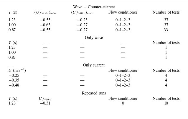
 T
 U¯
 clwo

 Hrms
 T=0.87s
 T=1.23s
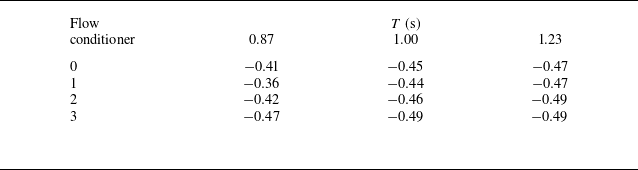
 U¯/clwo

 T=0.87s
 T=0.87s
 U/clwo=−0.27
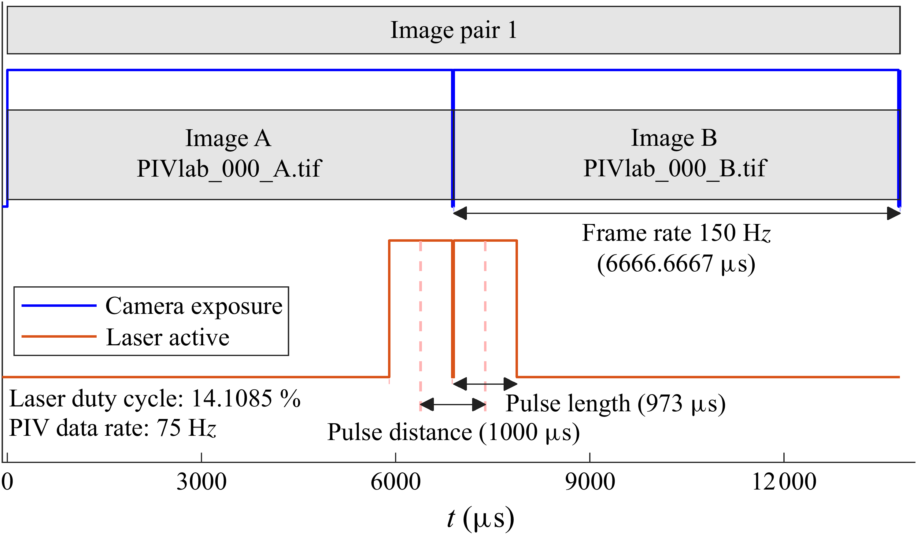


 T=1.23s
 U¯/clwo=−0.31

 T=1.23s
 U¯=−0.34m s−1

 T=1.23s
 H0=0.09m

 U¯=−0.27ms−1
 Δx=6

 Δx=141mm
 z/h∈[−0.78,0]
 T=1.23s
 U¯/clwo=−0.27
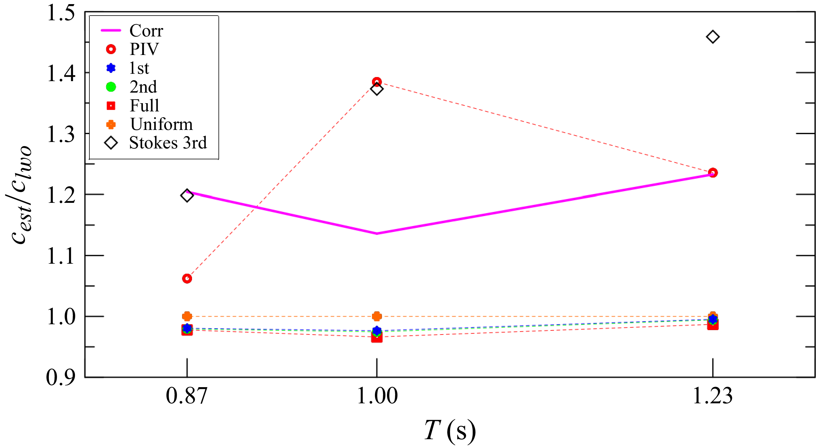
 cest
 clwo
 U(z)

 T=1.23s
 cest
 clwo

 T=1.00s

 T=0.87s

 δ(k)
 Δ(k)
 T=1.23s
 T=1.0s
 T=0.87s

 c1st/clwo
 c1st
 z=0
 δ
 z=0


 Open access

