1 Introduction
Several electrohydrodynamic studies have focused on the pillaring instability of a thin film subject to a constant DC electrical field. Wu & Chou (Reference Wu and Chou2003) developed a nonlinear lubrication model to successfully capture the pillaring instability observed in their experiments. Their model assumed a perfect dielectric film in contact with a hydrodynamically passive ambient phase. For general low-conducting fluids, charge accumulation and resulting stresses at the interface become important. Such fluids are described by the leaky dielectric (LD) theory developed by Melcher & Taylor (Reference Melcher and Taylor1969) and reviewed by Saville (Reference Saville1997). Shankar & Sharma (Reference Shankar and Sharma2004) analysed the linear stability of an active pair of LDs subject to normal electrical fields. They showed that pillaring length scales can be significantly altered by tuning the viscosity ratio of LD fluids. Ozen et al. (Reference Ozen, Aubry, Papageorgiou and Petropoulos2006) extended the stability analysis of a pair of LDs to the case of a channel flow. While earlier lubrication models that study pillar formation considered only one active fluid, Craster & Matar (Reference Craster and Matar2005) developed a lubrication model with active pair of LDs.
More recently, the effect of AC forcing on pillar formation has been investigated (Roberts & Kumar Reference Roberts and Kumar2009; Gambhire & Thaokar Reference Gambhire and Thaokar2010). While Gambhire & Thaokar (Reference Gambhire and Thaokar2010) investigated the influence of AC on the linear stability of the films, Roberts & Kumar (Reference Roberts and Kumar2009) used a nonlinear lubrication model to show that the height and spacing of the pillars can be controlled using AC forcing. In both works, mechanical inertia, hence resonance, is not considered. However, it is known since the early experiments of Faraday (Reference Faraday1831) that a fluid interface becomes unstable due to resonance when subject to parametric forcing. This forcing may be achieved in one of several ways, viz., mechanical motion of the fluid (Benjamin & Ursell Reference Benjamin and Ursell1954; Kumar & Tuckerman Reference Kumar and Tuckerman1994), imposing time-periodic electrostatic fields (Yih Reference Yih1968) or acoustic waves (Tsai & Tsai Reference Tsai and Tsai2013). The instability owes its origin to a resonant interaction between the forcing frequency and the natural frequency of the system. Interfacial patterns then typically arise subharmonic to the forcing frequency (Rayleigh Reference Rayleigh1833). However, in very thin liquid films of depth comparable to the viscous boundary layer, a harmonic response may be observed at the onset due to higher viscous dissipation associated with smaller wavenumbers in such films (Kumar Reference Kumar1996; Müller et al. Reference Müller, Wittmer, Wagner, Albers and Knorr1997). Usually, the natural frequency of the system owes its origin to the interaction between interfacial dynamics and fluid inertia, as was the case of Faraday’s fluid experiments. However, non-inertial effects such as fluid elasticity (Suman & Kumar Reference Suman and Kumar2008) or insoluble surfactant dynamics at the interface (Kumar & Matar Reference Kumar and Matar2002; Matar, Kumar & Craster Reference Matar, Kumar and Craster2004) may also result in a natural frequency and thereby a resulting resonant response. Electrostatically forced Faraday instability was first investigated by Briskman & Shaidurov (Reference Briskman and Shaidurov1968) and Yih (Reference Yih1968) who assumed an inviscid perfectly conducting fluid in contact with a perfect dielectric. This analysis was extended by Bandopadhyay & Hardt (Reference Bandopadhyay and Hardt2017) to include the effects of viscosity. Pillai & Narayanan (Reference Pillai and Narayanan2018) used an inertial lubrication model based on the long-wave theory to investigate the nonlinear evolution of the interface in such fluid pairs. Electrostatic Faraday instability in LD fluids was recently investigated by Ward, Matsumoto & Narayanan (Reference Ward, Matsumoto and Narayanan2019) and the predictions of the linear stability threshold were experimentally validated using water and silicone oil as working fluids. Papageorgiou (Reference Papageorgiou2019) presents a recent review of several electrohydrodynamic problems including pillar formation and electrostatically induced resonant instabilities.
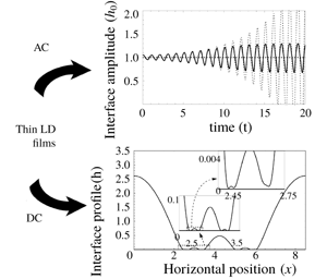
In the current work, an inertial lubrication model based on the weighted residual integral boundary layer (WRIBL) method (Ruyer-Quil & Manneville Reference Ruyer-Quil and Manneville2002) is developed for thin LD films. The focus of this work is on two distinct aspects of thin LD fluids subject to normal electrostatic forcing. First, we explore the resonant Faraday instability in thin inertial LD films, when subject to AC forcing. Two separate mechanisms of resonance arising due to fluid inertia and charge dynamics are elucidated. Second, we investigate the long-time dynamics of the pillaring interface under steady forcing as it approaches the wall. Specifically, we examine the long-time sliding and cascading structures exhibited by such thin films. To these ends, we present a mathematical model followed by discussions of various limiting cases.
2 Mathematical model
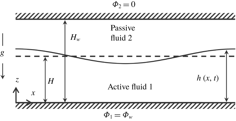
Consider a one-dimensional interface between a hydrodynamically active, Newtonian fluid 1 and a hydrodynamically passive fluid 2 (cf. figure 1). This implies that flow equations are solved only for fluid 1, while fluid 2 remains passive as far as flow is concerned. Electrostatic equations are, however, solved for both fluids 1 and 2. Although fluid 2 is treated as hydrodynamically passive in the current work, the physics of interfacial instability explored in this work are expected to qualitatively remain the same for a pair of hydrodynamically active fluids. A Cartesian coordinate system  $(x,z)$ is used where
 $x$ and
 $z$ denote the horizontal and vertical directions, respectively. The
 $x$ and
 $z$ component of the velocity vector
 $(\boldsymbol{v})$ are denoted by
 $u$ and
 $w$ respectively. Gravity acts in the negative
 $z$ direction. Fluid properties such as density, viscosity and surface tension are assumed to be constant and denoted by
 $\unicode[STIX]{x1D70C}$,
 $\unicode[STIX]{x1D707}$ and
 $\unicode[STIX]{x1D6FE}$. Both fluids are taken to be leaky dielectrics, i.e. the time scale for the charges to relax to the interface is assumed to be so short that they are confined to the fluid interface and the bounding wall (Saville Reference Saville1997). The upper wall at
 $z=H_{w}$ is grounded (
 $\unicode[STIX]{x1D6F7}_{2}=0$). The potential at the bottom wall (
 $z=0$) is held at
 $\unicode[STIX]{x1D6F7}_{1}=\unicode[STIX]{x1D6F7}_{w}$. For the case of AC forcing,
 $\unicode[STIX]{x1D6F7}_{w}=A\cos (\unicode[STIX]{x1D714}t)$, where
 $\unicode[STIX]{x1D714}=2\unicode[STIX]{x03C0}f$, and
 $f$ is the parametric forcing frequency, while for DC forcing,
 $\unicode[STIX]{x1D6F7}_{w}=A$, where
 $A$ is the magnitude of electric potential applied to the bottom wall. The long-wave approximation is used, i.e.
 $\unicode[STIX]{x1D6EC}$, the characteristic horizontal length scale due to instability, is taken to be much larger than the film thickness. Therefore, the ‘film parameter’,
 $\unicode[STIX]{x1D716}$, is introduced, which is defined as
 $\unicode[STIX]{x1D716}\equiv H/\unicode[STIX]{x1D6EC}\ll 1$.
Schematic of an interface between a pair of thin leaky dielectrics subject to normal electric field. Case 1 corresponds to the case of a periodic forcing, wherein  $\unicode[STIX]{x1D6F7}_{w}=A\cos (\unicode[STIX]{x1D714}t)$, while case 2 corresponds to a steady forcing, wherein
 $\unicode[STIX]{x1D6F7}_{w}=A$.

2.1 Governing equations
The equations governing flow for fluid 1 are the equations of continuity and Navier–Stokes given by
 $$\begin{eqnarray}\unicode[STIX]{x1D735}\boldsymbol{\cdot }\boldsymbol{v}_{1}=0\quad \text{and}\quad \unicode[STIX]{x1D70C}_{1}\left(\frac{\unicode[STIX]{x2202}\boldsymbol{v}_{1}}{\unicode[STIX]{x2202}t}+\boldsymbol{v}_{1}\boldsymbol{\cdot }\unicode[STIX]{x1D735}\boldsymbol{v}_{1}\right)=\unicode[STIX]{x1D735}\boldsymbol{\cdot }\unicode[STIX]{x1D64F}_{1}+\unicode[STIX]{x1D735}\boldsymbol{\cdot }\unicode[STIX]{x1D648}_{1}.\end{eqnarray}$$
In the above,  $\unicode[STIX]{x1D64F}_{1}=-p_{1}\unicode[STIX]{x1D644}+\unicode[STIX]{x1D707}_{1}(\unicode[STIX]{x1D735}\boldsymbol{v}_{1}+\unicode[STIX]{x1D735}\boldsymbol{v}_{1}^{\text{T}})$, is the usual Cauchy stress tensor, with
 $p_{1}$ denoting the isotropic fluid pressure,
 $\unicode[STIX]{x1D648}_{1}$ is the Maxwell stress tensor due to the electrical field (Saville Reference Saville1997), given by
 $\unicode[STIX]{x1D648}_{1}=\unicode[STIX]{x1D6FF}_{0}\unicode[STIX]{x1D6FF}_{1}[\boldsymbol{E}_{1}\boldsymbol{E}_{1}-1/2(\boldsymbol{E}_{1}\boldsymbol{\cdot }\boldsymbol{E}_{1})\unicode[STIX]{x1D644}]$, and
 $\unicode[STIX]{x1D644}$ is the identity tensor. Here,
 $\unicode[STIX]{x1D6FF}_{0}$ is the permittivity of the free space,
 $8.854\times 10^{-12}~\text{C}^{2}~\text{N}^{-1}~\text{m}^{-2}$, and
 $\unicode[STIX]{x1D6FF}_{1}$ is the dielectric constant of fluid 1. The electrical field in fluid
 $i$,
 $(\boldsymbol{E}_{i})$, expressed in terms of the potential gradient as
 $\boldsymbol{E}_{i}=-\unicode[STIX]{x1D735}\unicode[STIX]{x1D6F7}_{i}$, satisfies Gauss’ law. As discussed earlier, due to the low relaxation time associated with leaky dielectrics, the free charge in the bulk of either fluid is taken to be zero. Thus, we have the equations governing the electrical potential as follows:
 $$\begin{eqnarray}\unicode[STIX]{x1D6FB}^{2}\unicode[STIX]{x1D6F7}_{i}=0,\quad \text{subject to }\unicode[STIX]{x1D6F7}_{1}(0)=\unicode[STIX]{x1D6F7}_{w}\text{ and }\unicode[STIX]{x1D6F7}_{2}(H_{w})=0\text{ at the walls}.\end{eqnarray}$$
As  $\unicode[STIX]{x1D6FB}^{2}\unicode[STIX]{x1D6F7}_{i}=0$, it can be shown that the divergence of the Maxwell stress vanishes. Thus, the Maxwell stress term in (2.1b) is identically zero and it contributes only, but significantly, via the interfacial stress balance (2.3). At the interface (
 $z=h(x,t)$), the potentials in each phase are continuous and are related to the interfacial charge density (
 $Q$) as follows:
 $$\begin{eqnarray}\unicode[STIX]{x1D6F7}_{1}=\unicode[STIX]{x1D6F7}_{2}\quad \text{and}\quad \unicode[STIX]{x1D6FF}_{0}\unicode[STIX]{x1D6FF}_{2}\boldsymbol{E}_{2}\boldsymbol{\cdot }\boldsymbol{n}-\unicode[STIX]{x1D6FF}_{0}\unicode[STIX]{x1D6FF}_{1}\boldsymbol{E}_{1}\boldsymbol{\cdot }\boldsymbol{n}=Q.\end{eqnarray}$$
Equation (2.1e) is obtained by applying Gauss’ law to a differential volume containing the interface. The unit normal vector ( $\boldsymbol{n}$), the unit tangent vector (
 $\boldsymbol{t}$) and the interface normal speed (
 ${\mathcal{U}}$) are given by
 $$\begin{eqnarray}\boldsymbol{n}=\frac{-{\displaystyle \frac{\unicode[STIX]{x2202}h}{\unicode[STIX]{x2202}x}}\boldsymbol{i}_{x}+\boldsymbol{i}_{z}}{\left[1+\left({\displaystyle \frac{\unicode[STIX]{x2202}h}{\unicode[STIX]{x2202}x}}\right)^{2}\right]^{1/2}},\quad \boldsymbol{t}=\frac{\boldsymbol{i}_{x}+{\displaystyle \frac{\unicode[STIX]{x2202}h}{\unicode[STIX]{x2202}x}}\boldsymbol{i}_{z}}{\left[1+\left({\displaystyle \frac{\unicode[STIX]{x2202}h}{\unicode[STIX]{x2202}x}}\right)^{2}\right]^{1/2}}\quad \text{and}\quad {\mathcal{U}}=\frac{{\displaystyle \frac{\unicode[STIX]{x2202}h}{\unicode[STIX]{x2202}t}}}{\left[1+\left({\displaystyle \frac{\unicode[STIX]{x2202}h}{\unicode[STIX]{x2202}x}}\right)^{2}\right]^{1/2}}.\end{eqnarray}$$
The kinematic condition at the material interface between the immiscible fluids ensures that  $\boldsymbol{v}_{1}\boldsymbol{\cdot }\boldsymbol{n}-{\mathcal{U}}=0$ must hold. The interfacial stress balances are given by
 $$\begin{eqnarray}\boldsymbol{n}\boldsymbol{\cdot }\unicode[STIX]{x1D64F}_{1}\boldsymbol{\cdot }\boldsymbol{t}=Q\boldsymbol{E}\boldsymbol{\cdot }\boldsymbol{t}\quad \text{and}\quad \boldsymbol{n}\boldsymbol{\cdot }\unicode[STIX]{x1D64F}_{1}\boldsymbol{\cdot }\boldsymbol{n}+\boldsymbol{n}\boldsymbol{\cdot }(\unicode[STIX]{x1D648}_{1}-\unicode[STIX]{x1D648}_{2})\boldsymbol{\cdot }\boldsymbol{n}=-\unicode[STIX]{x1D6FE}\unicode[STIX]{x1D735}_{s}\boldsymbol{\cdot }\boldsymbol{n}.\end{eqnarray}$$
In the above, (2.3a) denotes the tangential stress balance, while (2.3b) denotes the normal stress balance. The right-hand side of the tangential stress balance represents the charge-induced shear stress due to the tangential component of Maxwell stress at the interface. Here,  $\unicode[STIX]{x1D648}_{2}=\unicode[STIX]{x1D6FF}_{0}\unicode[STIX]{x1D6FF}_{2}[\boldsymbol{E}_{2}\boldsymbol{E}_{2}-1/2(\boldsymbol{E}_{2}\boldsymbol{\cdot }\boldsymbol{E}_{2})\unicode[STIX]{x1D644}]$ is the Maxwell stress tensor corresponding to fluid 2. As can be seen from (2.3), the electrostatic contribution to the normal stress at the interface arises due to a jump in the normal component of the Maxwell stress at the interface.
The interfacial charge conservation (Saville Reference Saville1997), after incorporating corrections to surface charge density due to the motion of the interface as given by Johns (Reference Johns2016) is
 $$\begin{eqnarray}\left(\frac{\unicode[STIX]{x2202}Q}{\unicode[STIX]{x2202}t}+u\frac{\unicode[STIX]{x2202}Q}{\unicode[STIX]{x2202}x}-Q(\boldsymbol{n}\boldsymbol{\cdot }\boldsymbol{v})2{\mathcal{H}}-Q\boldsymbol{n}\boldsymbol{\cdot }(\boldsymbol{n}\boldsymbol{\cdot }\unicode[STIX]{x1D735})\boldsymbol{v}_{1}\right)=\unicode[STIX]{x1D70E}_{1}\boldsymbol{E}_{1}\boldsymbol{\cdot }\boldsymbol{n}-\unicode[STIX]{x1D70E}_{2}\boldsymbol{E}_{2}\boldsymbol{\cdot }\boldsymbol{n}.\end{eqnarray}$$
The left-hand side is the Lagrangian variation of the surface charge as one follows a parcel of fluid at the interface, while the right-hand side accounts for the electric current (rate of flow of charges) across the interface from the bulk. In the above,  $\unicode[STIX]{x1D70E}_{i}$ denotes the conductivity of fluid
 $i$ and
 $2{\mathcal{H}}$ is twice the local mean curvature.
2.2 Long-wave model
The following characteristic scales, denoted by the subscript ‘c’, are used for non-dimensionalization:
 $$\begin{eqnarray}\displaystyle & \displaystyle x_{c}=\unicode[STIX]{x1D6EC},\quad z_{c}=H,\quad u_{c}=U,\quad w_{c}=\unicode[STIX]{x1D716}U,\quad t_{c}=\unicode[STIX]{x1D6EC}/U, & \displaystyle \nonumber\\ \displaystyle & \displaystyle p_{c}=\unicode[STIX]{x1D707}_{1}U/H,\quad \unicode[STIX]{x1D6F7}_{i,c}=A,\quad Q_{c}=\unicode[STIX]{x1D6FF}_{0}\unicode[STIX]{x1D6FF}_{2}A/H. & \displaystyle \nonumber\end{eqnarray}$$
The velocity scale,  $U$, for AC forcing is obtained from the forcing frequency, i.e.
 $U=\unicode[STIX]{x1D714}H/2\unicode[STIX]{x03C0}$. For DC forcing,
 $U$ is obtained by a balance of the pressure term and the capillary term in the interfacial normal stress balance to give
 $U=\unicode[STIX]{x1D716}^{2}\unicode[STIX]{x1D6FE}/\unicode[STIX]{x1D707}_{1}$. The non-dimensional flow equations, retaining terms only up to
 $O(\unicode[STIX]{x1D716})$ are then obtained as
 $$\begin{eqnarray}\frac{\unicode[STIX]{x2202}u_{1}}{\unicode[STIX]{x2202}x}+\frac{\unicode[STIX]{x2202}w_{1}}{\unicode[STIX]{x2202}z}=0,\quad -\unicode[STIX]{x1D716}\frac{\unicode[STIX]{x2202}p_{1}}{\unicode[STIX]{x2202}z}-\unicode[STIX]{x1D716}G=0,\quad \text{where }G=\frac{\unicode[STIX]{x1D70C}_{1}gH^{2}}{\unicode[STIX]{x1D707}_{1}U},\quad \text{and}\end{eqnarray}$$
 $$\begin{eqnarray}\unicode[STIX]{x1D716}Re\left(\frac{\unicode[STIX]{x2202}u_{1}}{\unicode[STIX]{x2202}t}+u_{1}\frac{\unicode[STIX]{x2202}u_{1}}{\unicode[STIX]{x2202}x}+w_{1}\frac{\unicode[STIX]{x2202}u_{1}}{\unicode[STIX]{x2202}z}\right)=-\unicode[STIX]{x1D716}\frac{\unicode[STIX]{x2202}p_{1}}{\unicode[STIX]{x2202}x}+\frac{\unicode[STIX]{x2202}^{2}u_{1}}{\unicode[STIX]{x2202}z^{2}},\quad \text{where }Re=\frac{\unicode[STIX]{x1D70C}_{1}\,UH}{\unicode[STIX]{x1D707}_{1}}.\end{eqnarray}$$
To obtain the above equations,  $Re$ is taken to be
 $O(1)$, while
 $G$ to be at least
 $O(1)$. The no-slip and no-penetration conditions are given as
 $u_{1}(0)=w_{1}(0)=0$.
In the long-wave limit, equations (2.1c) and (2.1d,e) governing the potential for each phase reduce to  $\unicode[STIX]{x2202}^{2}\unicode[STIX]{x1D6F7}_{i}/\unicode[STIX]{x2202}z^{2}=0$, subject to the boundary conditions
 $$\begin{eqnarray}\unicode[STIX]{x1D6F7}_{1}(0)=\unicode[STIX]{x1D6F7}_{w},\quad \unicode[STIX]{x1D6F7}_{2}(\unicode[STIX]{x1D6FD})=0,\quad \unicode[STIX]{x1D6F7}_{1}(h)=\unicode[STIX]{x1D6F7}_{2}(h)\quad \text{and}\quad \unicode[STIX]{x1D6FF}\frac{\unicode[STIX]{x2202}\unicode[STIX]{x1D6F7}_{1}}{\unicode[STIX]{x2202}z}(h)-\frac{\unicode[STIX]{x2202}\unicode[STIX]{x1D6F7}_{2}}{\unicode[STIX]{x2202}z}(h)=Q.\end{eqnarray}$$
Here,  $\unicode[STIX]{x1D6FD}=H_{w}/H$,
 $\unicode[STIX]{x1D6FF}=\unicode[STIX]{x1D6FF}_{1}/\unicode[STIX]{x1D6FF}_{2}$ and
 $\unicode[STIX]{x1D6F7}_{w}$ is the scaled bottom wall potential and takes a value of 1 and
 $\cos (2\unicode[STIX]{x03C0}t)$ for DC and AC forcing respectively. Using (2.7), we can solve for the potential in each phase as
 $$\begin{eqnarray}\unicode[STIX]{x1D6F7}_{1}=\unicode[STIX]{x1D6F7}_{w}-z\left[\frac{\unicode[STIX]{x1D6F7}_{w}-Q(\unicode[STIX]{x1D6FD}-h)}{h+\unicode[STIX]{x1D6FF}(\unicode[STIX]{x1D6FD}-h)}\right]\quad \text{and}\quad \unicode[STIX]{x1D6F7}_{2}=(\unicode[STIX]{x1D6FD}-z)\left[\frac{\unicode[STIX]{x1D6FF}\unicode[STIX]{x1D6F7}_{w}+Qh}{h+\unicode[STIX]{x1D6FF}(\unicode[STIX]{x1D6FD}-h)}\right].\end{eqnarray}$$
The interfacial stress balance at  $z=h$ gives
 $$\begin{eqnarray}\frac{\unicode[STIX]{x2202}u_{1}}{\unicode[STIX]{x2202}z}=-\unicode[STIX]{x1D716}EE^{\text{T}}\quad \text{and}\quad p_{1}=\frac{E}{2}\left\{\unicode[STIX]{x1D6FF}\left(\frac{\unicode[STIX]{x2202}\unicode[STIX]{x1D6F7}_{1}}{\unicode[STIX]{x2202}z}\right)^{2}-\left(\frac{\unicode[STIX]{x2202}\unicode[STIX]{x1D6F7}_{2}}{\unicode[STIX]{x2202}z}\right)^{2}\right\}-\frac{\unicode[STIX]{x1D716}^{2}}{Ca}\frac{\unicode[STIX]{x2202}^{2}h}{\unicode[STIX]{x2202}x^{2}},\end{eqnarray}$$
where
 $$\begin{eqnarray}E=\frac{\unicode[STIX]{x1D6FF}_{0}\unicode[STIX]{x1D6FF}_{2}A^{2}}{\unicode[STIX]{x1D707}_{1}UH},\quad E^{\text{T}}=Q\left(\frac{\unicode[STIX]{x2202}\unicode[STIX]{x1D6F7}_{1}}{\unicode[STIX]{x2202}x}+\frac{\unicode[STIX]{x2202}\unicode[STIX]{x1D6F7}_{1}}{\unicode[STIX]{x2202}z}\frac{\unicode[STIX]{x2202}h}{\unicode[STIX]{x2202}x}\right),\quad Ca=\unicode[STIX]{x1D707}_{1}U/\unicode[STIX]{x1D6FE}.\end{eqnarray}$$
In the above,  $Ca$ is
 $O(\unicode[STIX]{x1D716}^{2})$, which corresponds to the large surface tension limit, valid for most fluids such as water and conducting polymers. This order of magnitude constraint on
 $Ca$ justifies our choice of velocity scale used in the case of steady DC forcing. In addition,
 $E$ is taken to be at least
 $O(1)$.
Integrating the continuity equation across the liquid film thickness and using the kinematic condition, we obtain  $\unicode[STIX]{x2202}h/\unicode[STIX]{x2202}t=-\unicode[STIX]{x2202}q/\unicode[STIX]{x2202}x$, where the flow rate is
 $q=\int _{0}^{h}u_{1}\,\text{d}z$. Integrating the vertical component of the momentum balance and eliminating pressure using (2.6) and (2.9), we obtain
 $$\begin{eqnarray}\unicode[STIX]{x1D716}Re\left(\frac{\unicode[STIX]{x2202}u_{1}}{\unicode[STIX]{x2202}t}+u_{1}\frac{\unicode[STIX]{x2202}u_{1}}{\unicode[STIX]{x2202}x}+w_{1}\frac{\unicode[STIX]{x2202}u_{1}}{\unicode[STIX]{x2202}z}\right)=\frac{\unicode[STIX]{x2202}^{2}u_{1}}{\unicode[STIX]{x2202}z^{2}}-\unicode[STIX]{x1D716}\left(EE^{N}+G\frac{\unicode[STIX]{x2202}h}{\unicode[STIX]{x2202}x}\right)+\frac{\unicode[STIX]{x1D716}^{3}}{Ca}\frac{\unicode[STIX]{x2202}^{3}h}{\unicode[STIX]{x2202}x^{3}},\end{eqnarray}$$
where  $E^{N}=\frac{1}{2}(\unicode[STIX]{x2202}/\unicode[STIX]{x2202}x)\{\unicode[STIX]{x1D6FF}(\unicode[STIX]{x2202}\unicode[STIX]{x1D6F7}_{1}/\unicode[STIX]{x2202}z)^{2}-(\unicode[STIX]{x2202}\unicode[STIX]{x1D6F7}_{2}/\unicode[STIX]{x2202}z)^{2}\}$. The interfacial charge equation, (2.4), under the long-wave approximation, reduces to
 $$\begin{eqnarray}\unicode[STIX]{x1D716}\unicode[STIX]{x1D712}\left[\frac{\unicode[STIX]{x2202}Q}{\unicode[STIX]{x2202}t}+\frac{\unicode[STIX]{x2202}}{\unicode[STIX]{x2202}x}(u_{1}|_{h}Q)\right]=\left(\frac{\unicode[STIX]{x2202}\unicode[STIX]{x1D6F7}_{2}}{\unicode[STIX]{x2202}z}-\unicode[STIX]{x1D70E}\frac{\unicode[STIX]{x2202}\unicode[STIX]{x1D6F7}_{1}}{\unicode[STIX]{x2202}z}\right),\quad \text{where }\unicode[STIX]{x1D70E}=\frac{\unicode[STIX]{x1D70E}_{1}}{\unicode[STIX]{x1D70E}_{2}},\unicode[STIX]{x1D712}=\frac{\unicode[STIX]{x1D6FF}_{0}\unicode[STIX]{x1D6FF}_{2}U}{\unicode[STIX]{x1D70E}_{2}H}.\end{eqnarray}$$
In the above,  $\unicode[STIX]{x1D712}$ is then the ratio of two time scales, viz., the charge relaxation time (
 $\unicode[STIX]{x1D6FF}_{0}\unicode[STIX]{x1D6FF}_{2}/\unicode[STIX]{x1D70E}_{2}$) and the fluid flow time scale (
 $H/U$).
Next, we follow the weighted residual technique developed by Ruyer-Quil & Manneville (Reference Ruyer-Quil and Manneville2002) and adopted by Pillai & Narayanan (Reference Pillai and Narayanan2018) to derive a set of reduced-order evolution equations that govern the interface position,  $h(x,t)$, flow rate,
 $q(x,t)$, and interfacial charge density,
 $Q(x,t)$. A weighted integral of the boundary layer equation (2.10) across the film thickness with an appropriate weight function is carried out. We begin by decomposing the horizontal velocity component as follows:
 $$\begin{eqnarray}u_{1}(x,z,t)=\hat{u} _{1}(x,z,t)+\tilde{u} _{1}(x,z,t),\quad {\hat{w}}_{1}=-\int _{0}^{z}\frac{\unicode[STIX]{x2202}\hat{u} _{1}}{\unicode[STIX]{x2202}x}\,\text{d}z.\end{eqnarray}$$
The hatted variable is of  $O(1)$, while tilde variable denotes the corresponding
 $O(\unicode[STIX]{x1D716})$ correction. The vertical component of velocity (
 $w_{1}$) is obtained from the continuity equation as shown. Next, the
 $O(1)$ contribution to the horizontal velocity components are chosen to satisfy the following conditions:
 $$\begin{eqnarray}\frac{\unicode[STIX]{x2202}^{2}\hat{u} _{1}}{\unicode[STIX]{x2202}z^{2}}=K_{v}(x,t),\quad \int _{0}^{h}\hat{u} _{1}\,\text{d}z=q(x,t),\quad \hat{u} _{1}|_{0}=0,\quad \left.\frac{\unicode[STIX]{x2202}\hat{u} _{1}}{\unicode[STIX]{x2202}z}\right|_{h}=0.\end{eqnarray}$$
Here,  $K_{v}(x,t)$ is introduced to ensure the leading-order velocity profile is locally semi-parabolic. The semi-parabolic velocity profile is justified for moderate Reynolds numbers. By definition, the
 $O(\unicode[STIX]{x1D716})$ correction to velocity (
 $\tilde{u}$) is required to satisfy
 $$\begin{eqnarray}\int _{0}^{h}\tilde{u} _{1}\,\text{d}z=0,\quad \tilde{u} _{1}|_{0}=0,\quad \left.\frac{\unicode[STIX]{x2202}\tilde{u} _{1}}{\unicode[STIX]{x2202}z}\right|_{h}=-\unicode[STIX]{x1D716}EE^{\text{T}}.\end{eqnarray}$$
Next, we substitute for velocity as given by (2.12) and the weighted residual integral of the boundary layer equation (2.10) is carried out. To obtain the evolution equations in terms of the variables  $h$,
 $q$,
 $Q$ alone, the unknown
 $\tilde{u} _{1}$ needs to be eliminated. In accordance with our first-order approximation, all terms of
 $O(\unicode[STIX]{x1D716}\tilde{u} _{1})=O(\unicode[STIX]{x1D716}^{2})$ and smaller are automatically dropped. The only term that still contains the
 $O(\unicode[STIX]{x1D716})$ correction is due to the viscous diffusion (i.e. the first term on the right-hand side of (2.10)). This term is eliminated by a suitable choice of weight function (
 $F$) as given by
 $$\begin{eqnarray}\frac{\unicode[STIX]{x2202}^{2}F}{\unicode[STIX]{x2202}z^{2}}=1,\quad F|_{0}=0,\quad \left.\frac{\unicode[STIX]{x2202}F}{\unicode[STIX]{x2202}z}\right|_{h}=0.\end{eqnarray}$$
The weighted integral of (2.10) across the film thickness, with the weight function ( $F$) as given by (2.15), yields the dynamic equation for the flow rate,
 $q$. The substitution of
 $\hat{u} _{1}$ in the left-hand side of (2.11) then directly gives the evolution equation for surface charge density,
 $Q$. The reduced-order model obtained after renormalizing the characteristic length scales, following Dietze & Ruyer-Quil (Reference Dietze and Ruyer-Quil2013), by setting
 $\unicode[STIX]{x1D716}=1$, is obtained as
 $$\begin{eqnarray}\displaystyle & \displaystyle \frac{\unicode[STIX]{x2202}h}{\unicode[STIX]{x2202}t}+\frac{\unicode[STIX]{x2202}q}{\unicode[STIX]{x2202}x}=0, & \displaystyle\end{eqnarray}$$
 $$\begin{eqnarray}\displaystyle & \hspace{-30.00005pt}\displaystyle Re\left(\frac{\unicode[STIX]{x2202}q}{\unicode[STIX]{x2202}t}+\frac{17q}{7h}\frac{\unicode[STIX]{x2202}q}{\unicode[STIX]{x2202}x}-\frac{9q^{2}}{7h^{2}}\frac{\unicode[STIX]{x2202}h}{\unicode[STIX]{x2202}x}\right)=-\frac{5q}{2h^{2}}-\frac{5}{4}EE^{\text{T}}+\frac{5h}{6}\left[\frac{1}{Ca}\frac{\unicode[STIX]{x2202}^{3}h}{\unicode[STIX]{x2202}x^{3}}-G\frac{\unicode[STIX]{x2202}h}{\unicode[STIX]{x2202}x}-EE^{N}\right], & \displaystyle\end{eqnarray}$$
 $$\begin{eqnarray}\displaystyle & \displaystyle \unicode[STIX]{x1D712}\left[\frac{\unicode[STIX]{x2202}Q}{\unicode[STIX]{x2202}t}+\frac{\unicode[STIX]{x2202}}{\unicode[STIX]{x2202}x}\left(\frac{3q}{2h}Q\right)\right]=\frac{\unicode[STIX]{x2202}\unicode[STIX]{x1D6F7}_{2}}{\unicode[STIX]{x2202}z}-\unicode[STIX]{x1D70E}\frac{\unicode[STIX]{x2202}\unicode[STIX]{x1D6F7}_{1}}{\unicode[STIX]{x2202}z}. & \displaystyle\end{eqnarray}$$
3 Limiting forms of the LD model
In this section, we derive the simplified forms of the LD model (2.16) for periodic and steady forcing under various limiting conditions. The limiting conditions are chosen, taking into consideration the particular physics of interest, under the different forms of forcing. As discussed earlier, the focus is on resonant instability in case of AC forcing, while for DC forcing, the focus is on the long-time dynamics such as spontaneous sliding and cascading structures of the interface near the wall.
3.1 Limiting forms of LD model under periodic forcing
Pair of perfect dielectrics
We first examine the limit when both fluids are perfect dielectrics of negligible conductivity, i.e.  $\unicode[STIX]{x1D70E}_{i}\rightarrow 0$. Fluid pairs such as silicone oil–air form examples of such a system. In terms of non-dimensional parameters, this limit corresponds to
 $\unicode[STIX]{x1D712}\rightarrow \infty$, with
 $\unicode[STIX]{x1D70E}$ (i.e. the ratio of conductivities) being finite. To consistently arrive at the perfect dielectric limit, it is further required to set the interfacial charge,
 $Q$ to zero, as was shown by Shankar & Sharma (Reference Shankar and Sharma2004). Equation (2.16c) is then trivially satisfied and (2.16b), after substituting for
 $\unicode[STIX]{x1D6F7}_{i}$ from (2.8) with
 $Q=0$, simplifies to
 $$\begin{eqnarray}\displaystyle & & \displaystyle Re\left(\frac{\unicode[STIX]{x2202}q}{\unicode[STIX]{x2202}t}+\frac{17q}{7h}\frac{\unicode[STIX]{x2202}q}{\unicode[STIX]{x2202}x}-\frac{9q^{2}}{7h^{2}}\frac{\unicode[STIX]{x2202}h}{\unicode[STIX]{x2202}x}\right)\nonumber\\ \displaystyle & & \displaystyle \quad =-\frac{5q}{2h^{2}}+\frac{5h}{6}\left(\frac{1}{Ca}\frac{\unicode[STIX]{x2202}^{3}h}{\unicode[STIX]{x2202}x^{3}}-G\frac{\unicode[STIX]{x2202}h}{\unicode[STIX]{x2202}x}+\frac{E\unicode[STIX]{x1D6FF}(\unicode[STIX]{x1D6FF}-1)^{2}}{2}\frac{[1+\cos (4\unicode[STIX]{x03C0}t)]}{(\unicode[STIX]{x1D6FF}(\unicode[STIX]{x1D6FD}-h)+h)^{3}}\frac{\unicode[STIX]{x2202}h}{\unicode[STIX]{x2202}x}\right).\end{eqnarray}$$
It is evident from (3.1) that  $\unicode[STIX]{x1D6FF}\neq 1$ is a necessary condition for electrostatic forcing of perfect dielectric fluids. In other words, a disparity in permittivity is essential for a pair of perfect dielectrics to see any instability.
Perfect conductor–perfect dielectric pair
Another interesting limit is that of a perfectly conducting liquid in contact with a perfect dielectric, i.e.  $\unicode[STIX]{x1D70E}\rightarrow \infty$. In this case, (2.16c) simply reduces to
 $\unicode[STIX]{x2202}\unicode[STIX]{x1D6F7}_{1}/\unicode[STIX]{x2202}z=0$. This, along with (2.8), suggests that the potential in fluid 1 is independent of
 $z$ and given by
 $\unicode[STIX]{x1D6F7}_{1}=\cos (2\unicode[STIX]{x03C0}t)$, with the interfacial charge density being
 $Q=\cos (2\unicode[STIX]{x03C0}t)/(\unicode[STIX]{x1D6FD}-h)$. Using this expression for
 $Q$ in (2.8), we obtain
 $\unicode[STIX]{x1D6F7}_{2}=\cos (2\unicode[STIX]{x03C0}t)[(\unicode[STIX]{x1D6FD}-z)/(\unicode[STIX]{x1D6FD}-h)]$ and the WRIBL model reduces to just (2.16a) along with the following evolution equation for flow rate,
 $q$:
 $$\begin{eqnarray}\displaystyle & & \displaystyle Re\left(\frac{\unicode[STIX]{x2202}q}{\unicode[STIX]{x2202}t}+\frac{17q}{7h}\frac{\unicode[STIX]{x2202}q}{\unicode[STIX]{x2202}x}-\frac{9q^{2}}{7h^{2}}\frac{\unicode[STIX]{x2202}h}{\unicode[STIX]{x2202}x}\right)\nonumber\\ \displaystyle & & \displaystyle \quad =-\frac{5q}{2h^{2}}+\frac{5h}{6}\left(\frac{1}{Ca}\frac{\unicode[STIX]{x2202}^{3}h}{\unicode[STIX]{x2202}x^{3}}-G\frac{\unicode[STIX]{x2202}h}{\unicode[STIX]{x2202}x}+\frac{E}{2}\frac{[1+\cos (4\unicode[STIX]{x03C0}t)]}{(\unicode[STIX]{x1D6FD}-h)^{3}}\frac{\unicode[STIX]{x2202}h}{\unicode[STIX]{x2202}x}\right).\end{eqnarray}$$
This limit is valid for fluid pairs such as ultra-purified water–air or liquid metal–air. Equation (3.2) is exactly as obtained by Pillai & Narayanan (Reference Pillai and Narayanan2018) for Faraday instability of thin liquid films for a perfect conducting–perfect dielectric pair. Note, however, that their definition of  $E$ differs from the current work by a factor of 1/2. It should be further noted that, under both limits hitherto discussed, charge dynamics plays no role. Therefore, in these cases, fluid inertia is essential for the system to have a natural frequency and thereby exhibit parametric resonance. Further, the instability is solely due to the normal component of Maxwell stress at the interface.
Leaky dielectrics with fast relaxation time
A convenient model to understand the role of surface charge induced stresses on the interfacial dynamics is to examine (2.16) in the limit of fast relaxation time, i.e.  $\unicode[STIX]{x1D712}<<1$ (Papageorgiou & Petropoulos Reference Papageorgiou and Petropoulos2004; Uguz, Ozen & Aubry Reference Uguz, Ozen and Aubry2008; Wray et al. Reference Wray, Matar and Papageorgiou2017). Under this limit, the left-hand side of (2.16c) is dropped altogether and it then serves as a constraint required to be satisfied by the electrical potential at the interface. Substituting for the potential so obtained from (2.16c) in (2.16b), the WRIBL model reduces to (2.16a) along with the following equation governing the flow rate,
 $q$:

From the above, it is clear that for this case there are two contributions due to the applied electric field, one arising due to charge-induced tangential stress at the interface, while the other is due to the normal component of the Maxwell stress.
Inertialess leaky dielectrics
Next, we examine (2.16) in the limit of no inertia, i.e.  $Re\rightarrow 0$. Under this limit, the flow rate,
 $q$, can be obtained as a functional of
 $h$ and
 $Q$ from (2.16b). Thus, eliminating
 $q$ from (2.16a) and (2.16c), we obtain two evolution equations for
 $h$ and
 $Q$ alone as follows:
 $$\begin{eqnarray}\displaystyle & \displaystyle \frac{\unicode[STIX]{x2202}h}{\unicode[STIX]{x2202}t}=\frac{\unicode[STIX]{x2202}}{\unicode[STIX]{x2202}x}\left[\frac{h^{2}}{2}EE^{\text{T}}-\frac{h^{3}}{3}\left(\frac{1}{Ca}\frac{\unicode[STIX]{x2202}^{3}h}{\unicode[STIX]{x2202}x^{3}}-G\frac{\unicode[STIX]{x2202}h}{\unicode[STIX]{x2202}x}-EE^{N}\right)\right] & \displaystyle\end{eqnarray}$$
 $$\begin{eqnarray}\displaystyle & \displaystyle \unicode[STIX]{x1D712}\left[\frac{\unicode[STIX]{x2202}Q}{\unicode[STIX]{x2202}t}+\frac{\unicode[STIX]{x2202}}{\unicode[STIX]{x2202}x}\left(\frac{3q}{2h}Q\right)\right]=\frac{\unicode[STIX]{x2202}\unicode[STIX]{x1D6F7}_{2}}{\unicode[STIX]{x2202}z}-\unicode[STIX]{x1D70E}\frac{\unicode[STIX]{x2202}\unicode[STIX]{x1D6F7}_{1}}{\unicode[STIX]{x2202}z}. & \displaystyle\end{eqnarray}$$
This limit helps us to drop the role of inertia and explore the possibility of an inertialess Faraday instability in LD fluids brought into effect solely due to interaction between interfacial kinematics and charge dynamics. Finally, the general inertial LD model allows for Faraday response due to the combined action of charge dynamics and fluid inertia, as we shall see.
3.2 Limiting forms of LD model under steady forcing
In this section, we derive various limiting forms of the LD model subject to steady forcing, with our primary interest being the long-time dynamics of the interface prior to rupture. Due to very thin configurations attained by a fluid film under these conditions, inertial effects become unimportant, as was shown by Dietze, Picardo & Narayanan (Reference Dietze, Picardo and Narayanan2018). Therefore, we consider the limit of vanishing inertia, i.e.  $Re\rightarrow 0$. Further, it is known that gravity is unimportant in the long-time drainage of thin films near the wall (Lister, Rallison & Rees Reference Lister, Rallison and Rees2010; Dietze et al. Reference Dietze, Picardo and Narayanan2018). Thus, we also set non-dimensional gravity,
 $G\rightarrow 0$.
Pair of perfect dielectrics
We first examine the limit where both fluids are perfect dielectrics of negligible conductivity. Equation (2.16c) is then trivially satisfied and (2.16b), simplifies to
 $$\begin{eqnarray}q=\frac{h^{3}}{3}\left(\frac{1}{Ca}\frac{\unicode[STIX]{x2202}^{3}h}{\unicode[STIX]{x2202}x^{3}}+\frac{E\unicode[STIX]{x1D6FF}(\unicode[STIX]{x1D6FF}-1)^{2}}{(\unicode[STIX]{x1D6FF}(\unicode[STIX]{x1D6FD}-h)+h)^{3}}\frac{\unicode[STIX]{x2202}h}{\unicode[STIX]{x2202}x}\right).\end{eqnarray}$$
As was the case with AC forcing, it is evident from (3.5) that  $\unicode[STIX]{x1D6FF}\neq 1$ is a necessary condition for instability in perfect dielectric fluids, as was also shown by Shankar & Sharma (Reference Shankar and Sharma2004). It is important to note here that the model obtained above in (3.5) is similar to the classical lubrication model for Rayleigh–Taylor instability. There, the contributions to the flow rate (
 $q$) are due to gravity and capillarity (cf. Lister, Morrison & Rallison (Reference Lister, Morrison and Rallison2006a) and Dietze et al. (Reference Dietze, Picardo and Narayanan2018)) and reproduced here in terms of the current scaling as
 $$\begin{eqnarray}q=\frac{h^{3}}{3}\left(\frac{1}{Ca}\frac{\unicode[STIX]{x2202}^{3}h}{\unicode[STIX]{x2202}x^{3}}+G\frac{\unicode[STIX]{x2202}h}{\unicode[STIX]{x2202}x}\right),\quad \text{where }G=\frac{\unicode[STIX]{x1D70C}gH^{2}}{\unicode[STIX]{x1D707}U}.\end{eqnarray}$$
Comparing (3.5) and (3.6), it is evident that for low liquid hold-up ( $h\ll \unicode[STIX]{x1D6FD}$), the system is analogous to a Rayleigh–Taylor unstable system with the non-dimensional gravity,
 $G$ replaced by
 $E(\unicode[STIX]{x1D6FF}-1)^{2}/\unicode[STIX]{x1D6FF}^{2}\unicode[STIX]{x1D6FD}^{3}$, which is positive definite and therefore always destabilizing. It is therefore expected that the system exhibits the long-time sliding instability associated with thin Rayleigh–Taylor thin films reported by Lister et al. (Reference Lister, Morrison and Rallison2006a) and Dietze et al. (Reference Dietze, Picardo and Narayanan2018).
Perfect conductor–perfect dielectric pair
Next, we investigate the limit of a perfectly conducting liquid in contact with a perfect dielectric. The governing equations then consist of (2.16a) along with the simplified form of (2.16b), given by
 $$\begin{eqnarray}q=\frac{h^{3}}{3}\left(\frac{1}{Ca}\frac{\unicode[STIX]{x2202}^{3}h}{\unicode[STIX]{x2202}x^{3}}+\frac{E}{(\unicode[STIX]{x1D6FD}-h)^{3}}\frac{\unicode[STIX]{x2202}h}{\unicode[STIX]{x2202}x}\right).\end{eqnarray}$$
Examining (3.7), we see that, for low liquid hold-up ( $h\ll \unicode[STIX]{x1D6FD}$), the perfect conductor model is analogous to that of a Rayleigh–Taylor system with the non-dimensional gravity,
 $G$ replaced by
 $E/\unicode[STIX]{x1D6FD}^{3}$. It is therefore expected that an interface between a perfect conductor and a perfect dielectric also exhibits dynamics similar to a Rayleigh–Taylor unstable interface. It was indeed shown by Pillai & Narayanan (Reference Pillai and Narayanan2018) that a perfectly conducting thin film does exhibit long-time sliding dynamics. Under both the limits discussed above, charge dynamics at the interface plays no role and hence the interface is free of shear stress. The instability is then solely due to the normal component of Maxwell stress at the interface.
Leaky dielectrics with fast relaxation time
In the limit of fast relaxation time for steady forcing, we obtain the flow rate,  $q$, as
 $$\begin{eqnarray}q=\underbrace{\frac{h^{2}}{2}\frac{E\unicode[STIX]{x1D6FD}\unicode[STIX]{x1D70E}(\unicode[STIX]{x1D70E}-\unicode[STIX]{x1D6FF})}{(\unicode[STIX]{x1D70E}(\unicode[STIX]{x1D6FD}-h)+h)^{3}}\frac{\unicode[STIX]{x2202}h}{\unicode[STIX]{x2202}x}}_{\mathit{Tangential~stress},\,q|_{E^{\text{T}}}}+\frac{h^{3}}{3}\left(\underbrace{\frac{1}{Ca}\frac{\unicode[STIX]{x2202}^{3}h}{\unicode[STIX]{x2202}x^{3}}}_{\mathit{Capillarity},\,q|_{Ca}}+\underbrace{\frac{E(\unicode[STIX]{x1D70E}-1)(\unicode[STIX]{x1D70E}^{2}-\unicode[STIX]{x1D6FF})}{(\unicode[STIX]{x1D70E}(\unicode[STIX]{x1D6FD}-h)+h)^{3}}\frac{\unicode[STIX]{x2202}h}{\unicode[STIX]{x2202}x}}_{\mathit{Normal~stress},\,q|_{E^{N}}}\right).\end{eqnarray}$$
As is evident from (3.8), there are three contributions to the flow rate. The first term corresponds to flow generated by the tangential component of the Maxwell stress at the interface in the presence of interfacial charge. The last term corresponds to the flow due to a jump in the normal component of the fluid Maxwell stresses at the interface. The second term corresponds to flow due to interface curvature-driven capillary pressure. Equation (3.8) is reminiscent of the lubrication model for a Rayleigh–Taylor unstable interface with an additional thermal Marangoni stress due to heating of the bounding wall (cf. (2.3) in Dietze et al. (Reference Dietze, Picardo and Narayanan2018)). In (3.8), the term analogous to gravity is due to the normal component of Maxwell stress,  $q|_{E^{n}}$, while the tangential component of Maxwell stress,
 $q|_{E^{t}}$, results in flow analogous to the thermal Marangoni effect. For low liquid hold-up (
 $h\ll \unicode[STIX]{x1D6FD}$) and
 $\unicode[STIX]{x1D70E}>1$ (a valid assumption when the ambient medium is hydrodynamically passive), the system is analogous to a Rayleigh–Taylor unstable interface with an effective gravity,
 $G=E(\unicode[STIX]{x1D70E}-1)(\unicode[STIX]{x1D70E}^{2}-\unicode[STIX]{x1D6FF})/(\unicode[STIX]{x1D70E}\unicode[STIX]{x1D6FD})^{3}$. It is important to note that the flow due to capillarity (
 $q|_{Ca}$) and the normal Maxwell stress (
 $q|_{E^{n}}$) is modulated by viscous effects which scale as
 $h^{3}$, while the flow due to the tangential Maxwell stress
 $q|_{E^{t}}$ scales as
 $h^{2}$. Therefore, as the film progressively thins, i.e. with a decrease in
 $h$, the tangential stress dominates the normal stress. This is very similar to thermal Marangoni stresses dominating the role of buoyancy in the analogous problem studied by Dietze et al. (Reference Dietze, Picardo and Narayanan2018). Thus, we anticipate the long-time dynamics of a general LD film to be similar to their problem, wherein sliding was precluded and instead cascading structures were observed.
4 Results and discussion
We restrict our results to cases of low  $k$ to ensure that the wavelength is at least an order of magnitude larger than the film thickness and the long-wave approximation is upheld. We begin with the results of resonant instability in LD films under periodic forcing, followed by the long-time dynamics under steady forcing. In both cases, linear stability results are first presented and then nonlinear calculations are subsequently carried out.
For the case of periodic forcing, we perform a linear stability of (2.16) (cf. Nayfeh (Reference Nayfeh1981) for use of Floquet theory) as well as its various limits about a base state which is stationary with a flat interface. The variables are perturbed about the base state as  $h=\bar{h}+h^{\prime }(t)\exp [\text{i}kx]$, etc. Here,
 $\bar{h}=1$ denotes the base state, prime denotes the perturbed state and
 $k$ the wavenumber. Also,
 $\bar{q}=0$ and
 $\bar{Q}=\bar{C}_{1}\cos (2\unicode[STIX]{x03C0}t)+\bar{C}_{2}\sin (2\unicode[STIX]{x03C0}t)$, where
 $$\begin{eqnarray}\left.\begin{array}{@{}c@{}}\displaystyle \bar{C}_{1}=\frac{\unicode[STIX]{x1D712}^{2}(\unicode[STIX]{x1D70E}-\unicode[STIX]{x1D6FF})(1+\unicode[STIX]{x1D70E}(\unicode[STIX]{x1D6FD}-1))}{(\unicode[STIX]{x1D712}(1+\unicode[STIX]{x1D70E}(\unicode[STIX]{x1D6FD}-1)))^{2}+(2\unicode[STIX]{x03C0}(1+\unicode[STIX]{x1D6FF}(\unicode[STIX]{x1D6FD}-1)))^{2}},\\ \displaystyle \bar{C}_{2}=\frac{\unicode[STIX]{x1D712}^{2}(\unicode[STIX]{x1D70E}-\unicode[STIX]{x1D6FF})(1+\unicode[STIX]{x1D6FF}(\unicode[STIX]{x1D6FD}-1))}{(\unicode[STIX]{x1D712}(1+\unicode[STIX]{x1D70E}(\unicode[STIX]{x1D6FD}-1)))^{2}+(2\unicode[STIX]{x03C0}(1+\unicode[STIX]{x1D6FF}(\unicode[STIX]{x1D6FD}-1)))^{2}}.\end{array}\right\}\end{eqnarray}$$
It is to be noted from (4.1) that, for the special case of  $\unicode[STIX]{x1D70E}=\unicode[STIX]{x1D6FF}$, we obtain
 $\bar{Q}=0$.
For the case of steady forcing, linear stability analysis of the system under the various limits and perturbing about the flat base state as  $h=1+h^{\prime }\exp [\unicode[STIX]{x1D6FC}t+\text{i}kx]$ is performed. Here,
 $\unicode[STIX]{x1D6FC}$ is the linear temporal growth rate.
4.1 Resonant instability under periodic forcing
In this section, we discuss the results of resonant instability arising due to periodic forcing.
4.1.1 Linear stability analysis
Pair of perfect dielectrics
The perfect dielectric model is described by (2.16a) and (3.1). Upon linearization, we get a damped Mathieu equation, viz.,
 $$\begin{eqnarray}\displaystyle & \displaystyle \frac{\text{d}^{2}h^{\prime }}{\text{d}t^{2}}+\unicode[STIX]{x1D701}\frac{\text{d}h^{\prime }}{\text{d}t}+\left[\unicode[STIX]{x1D714}_{0}^{2}-\unicode[STIX]{x1D702}\cos (4\unicode[STIX]{x03C0}t)\right]h^{\prime }=0,\quad \text{where }\unicode[STIX]{x1D701}=\frac{5}{2Re}, & \displaystyle \nonumber\\ \displaystyle & \displaystyle \unicode[STIX]{x1D714}_{0}^{2}=\frac{5}{6Re}\left(Gk^{2}+\frac{1}{Ca}k^{4}-\frac{E\unicode[STIX]{x1D6FF}(\unicode[STIX]{x1D6FF}-1)^{2}k^{2}}{2(1+\unicode[STIX]{x1D6FF}(\unicode[STIX]{x1D6FD}-1))^{3}}\right),\quad \unicode[STIX]{x1D702}=\frac{5}{12Re}\frac{E\unicode[STIX]{x1D6FF}(\unicode[STIX]{x1D6FF}-1)^{2}k^{2}}{(1+\unicode[STIX]{x1D6FF}(\unicode[STIX]{x1D6FD}-1))^{3}}.\qquad & \displaystyle\end{eqnarray}$$
Here,  $\unicode[STIX]{x1D714}_{0}$ is the natural frequency and the Mathieu equation has a forcing frequency,
 $4\unicode[STIX]{x03C0}$, compared to the imposed parametric frequency,
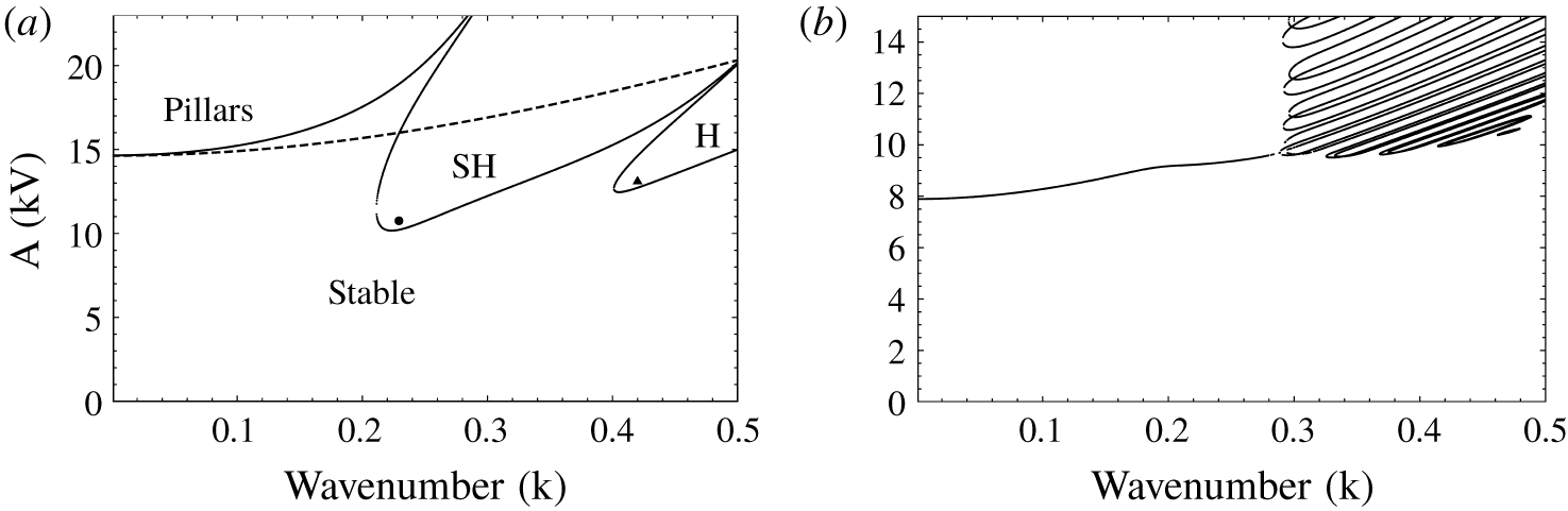
 $2\unicode[STIX]{x03C0}$, due to the quadratic dependence of the Maxwell stress on the electric field. Calculations are carried out using typical fluid properties of silicone oil and air (cf. table 1). In figure 2(a), the dashed line denotes the neutral curve obtained in the absence of inertia (
 $Re=0$) for such a thin liquid film. It is seen that the system becomes unstable beyond a critical value of the potential to a long-wave instability. This corresponds to the ‘pillaring’ instability reported by Wu & Chou (Reference Wu and Chou2003) and Roberts & Kumar (Reference Roberts and Kumar2009). The solid curve denotes the neutral stability curve in the presence of inertia. In the presence of inertia, the neutral curve exhibits additional ‘tongues’ corresponding to subharmonic (SH) and harmonic (H) responses. It should be noted that a subharmonic tongue in response to a parametric frequency of 2
 $\unicode[STIX]{x03C0}$ would elicit a response of 2
 $\unicode[STIX]{x03C0}$ itself, since the Maxwell stress experienced by the interface has a frequency of 4
 $\unicode[STIX]{x03C0}$. Likewise, a harmonic response shows a frequency of 4
 $\unicode[STIX]{x03C0}$. Since the critical threshold for these resonant modes is below that of the pillaring mode, Faraday modes are expected to be observed at the onset in experiments, when creeping up the amplitude of electrode potential.
(a) Neutral stability curve (solid) showing subharmonic (SH) and harmonic (H) Faraday tongues for perfect dielectric fluids. In the absence of inertia (dashed), only the ‘pillaring’ mode exists. Markers denote parameters chosen for nonlinear simulations in figure 4. (b) Neutral stability curve for inertialess LD fluids (cf. paragraph after (4.5) in the main text for discussion);  $H=0.75~\text{mm},\unicode[STIX]{x1D6FD}=5,f=3~\text{Hz}$.

Physical properties for the perfect dielectric pair of silicone oil and air (Ward et al. Reference Ward, Matsumoto and Narayanan2019) used in our calculations to obtain figure 2(a).

Perfect conductor–perfect dielectric pair
The limit of a perfect conductor–perfect dielectric fluid pair, investigated in earlier work (Pillai & Narayanan Reference Pillai and Narayanan2018), is described briefly here. In this case too, linearization of (2.16a) and (3.2) results in a damped Mathieu equation like (4.2), where now  $\unicode[STIX]{x1D714}_{0}^{2}$ and
 $\unicode[STIX]{x1D702}$ are as follows:
 $$\begin{eqnarray}\unicode[STIX]{x1D714}_{0}^{2}=\frac{5}{6Re}\left(Gk^{2}+\frac{1}{Ca}k^{4}-\frac{Ek^{2}}{2(\unicode[STIX]{x1D6FD}-1)^{3}}\right),\quad \unicode[STIX]{x1D702}=\frac{5}{12Re}\frac{Ek^{2}}{(\unicode[STIX]{x1D6FD}-1)^{3}}.\end{eqnarray}$$
The neutral stability curve shows alternating harmonic and subharmonic tongues, which respectively correspond to isosynchronous and a double-frequency response of the interface motion. It was also shown by Pillai & Narayanan (Reference Pillai and Narayanan2018) that fluid inertia is a necessary requirement to attain resonant modes of instability. We now proceed to discuss the limit of a pair of leaky dielectrics with fast relaxation time.
Leaky dielectrics with fast relaxation time
The limit of leaky dielectrics with fast relaxation time, (2.16a) and (3.3), also upon linearization, result in a damped Mathieu equation like (4.2) where now  $\unicode[STIX]{x1D714}_{0}^{2}$ and
 $\unicode[STIX]{x1D702}$ are as follows:
 $$\begin{eqnarray}\left.\begin{array}{@{}c@{}}\displaystyle \unicode[STIX]{x1D714}_{0}^{2}=\frac{5}{6Re}\left(Gk^{2}+\frac{1}{Ca}k^{4}-\underbrace{\frac{E(\unicode[STIX]{x1D70E}-1)(\unicode[STIX]{x1D70E}^{2}-\unicode[STIX]{x1D6FF})k^{2}}{2(\unicode[STIX]{x1D70E}(\unicode[STIX]{x1D6FD}-1)+1)^{3}}}_{\mathit{Normal~stress}}\right)-\underbrace{\frac{5}{8Re}\frac{E\unicode[STIX]{x1D6FD}\unicode[STIX]{x1D70E}(\unicode[STIX]{x1D70E}-\unicode[STIX]{x1D6FF})k^{2}}{(\unicode[STIX]{x1D70E}(\unicode[STIX]{x1D6FD}-1)+1)^{3}}}_{\mathit{Tangential~stress}},\\ \displaystyle \unicode[STIX]{x1D702}=\frac{5E}{4Re}\left(\frac{(\unicode[STIX]{x1D70E}-1)(\unicode[STIX]{x1D70E}^{2}-\unicode[STIX]{x1D6FF})k^{2}}{3(\unicode[STIX]{x1D70E}(\unicode[STIX]{x1D6FD}-1)+1)^{3}}+\frac{\unicode[STIX]{x1D6FD}\unicode[STIX]{x1D70E}(\unicode[STIX]{x1D70E}-\unicode[STIX]{x1D6FF})k^{2}}{2(\unicode[STIX]{x1D70E}(\unicode[STIX]{x1D6FD}-1)+1)^{3}}\right).\end{array}\right\}\end{eqnarray}$$
The natural frequency can be seen to be modified due to the normal component of Maxwell stress as well as the tangential component of the Maxwell stress arising due to finite charge density at the interface. Similar to the earlier cases, the neutral stability curve shows alternating harmonic and subharmonic tongues. The resonant instability in this case is also solely due to fluid inertia. We now proceed to discuss the limit of inertialess LD fluids.
Inertialess leaky dielectrics
Unlike the earlier cases, linearizing (2.16) in the limit of  $Re\rightarrow 0$ does not yield a simple Mathieu equation. Instead, we obtain two linear coupled equations for
 $h^{\prime }$ and
 $Q^{\prime }$ as given below
 $$\begin{eqnarray}\hspace{-5.0pt}\left.\begin{array}{@{}c@{}}\displaystyle \frac{\text{d}h^{\prime }}{\text{d}t}+[L_{1}+L_{2}\cos (4\unicode[STIX]{x03C0}t)+L_{3}\sin (4\unicode[STIX]{x03C0}t)]h^{\prime }+[L_{4}\cos (2\unicode[STIX]{x03C0}t)+L_{5}\sin (2\unicode[STIX]{x03C0}t)]Q^{\prime }=0\\ \displaystyle \frac{\text{d}Q^{\prime }}{\text{d}t}+[M_{1}\cos (2\unicode[STIX]{x03C0}t)+M_{2}\sin (2\unicode[STIX]{x03C0}t)]\frac{\text{d}h^{\prime }}{\text{d}t}\qquad \qquad \quad \\ \quad +\,[M_{3}\cos (2\unicode[STIX]{x03C0}t)+M_{4}\sin (2\unicode[STIX]{x03C0}t)]h^{\prime }+M_{5}Q^{\prime }=0,\end{array}\right\}\end{eqnarray}$$
where the parameters appearing in the above equation are lengthy expressions obtained via Mathematica and are given in the ancillary supplementary material (available at https://doi.org/10.1017/jfm.2020.112).
Physical properties for the leaky dielectric pair used in our calculations to obtain figure 2(b).

We perform calculations using the properties in table 2 for a pair of leaky dielectrics. The neutral stability curve for this case is depicted in figure 2(b). For low wavenumbers, the long-wave pillaring mode is observed. Interestingly, a clustered Faraday tongue structure exists for higher wavenumbers. These tongues correspond to a resonant Faraday mode arising from charge dynamics at the interface. It was observed that the critical amplitude corresponding to the onset of instability corresponds to a harmonic response for all of the cases studied. A very similar resonant tongue structure was observed by Kumar & Matar (Reference Kumar and Matar2002) and Matar et al. (Reference Matar, Kumar and Craster2004), albeit for a completely different physical problem, on a parametrically forced fluid with an insoluble surfactant at the interface. Similar to the interfacial charge dynamics in the current problem, it is the presence of interfacial solute dynamics that drives a Faraday response in their system. Our figure 2(b) is thus qualitatively very similar to those given in (Kumar & Matar Reference Kumar and Matar2002, figure 1) and Matar et al. (Reference Matar, Kumar and Craster2004). In fact, for a thin viscous liquid undergoing simple mechanical oscillation, it is known that the first subharmonic tongue gets shifted upward due to the larger dissipation associated with low wavenumbers in such fluids, and the harmonic tongue can become the most unstable (Kumar Reference Kumar1996). For significantly high damping, one may then observe clustered Faraday tongues very similar to that in figure 2(b). It was shown by Bestehorn (Reference Bestehorn2013) that the equation governing the linear stability of such a mechanically oscillated interface is a damped Mathieu equation (cf. their equation (52)) with
 $$\begin{eqnarray}\displaystyle & \displaystyle \frac{\text{d}^{2}h^{\prime }}{\text{d}t^{2}}+\unicode[STIX]{x1D701}\frac{\text{d}h^{\prime }}{\text{d}t}+\left[\unicode[STIX]{x1D714}_{0}^{2}-\unicode[STIX]{x1D702}\cos (2\unicode[STIX]{x03C0}t)\right]h^{\prime }=0 & \displaystyle \nonumber\\ \displaystyle & \displaystyle \text{where }\unicode[STIX]{x1D701}=\frac{5}{2Re},\quad \unicode[STIX]{x1D714}_{0}^{2}=\frac{5}{6Re}\left(Gk^{2}+\frac{1}{Ca}k^{4}\right),\quad \unicode[STIX]{x1D702}=\frac{\unicode[STIX]{x1D70C}_{1}{\mathcal{A}}\unicode[STIX]{x1D714}^{2}H^{2}}{\unicode[STIX]{x1D707}_{1}U}. & \displaystyle\end{eqnarray}$$
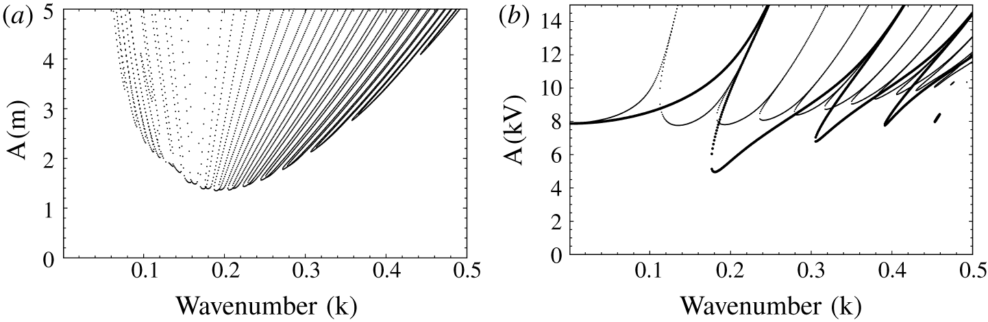
In the above,  ${\mathcal{A}}$ is the amplitude of mechanical motion. The neutral stability curve for a thin mechanically oscillated water film in contact with hydrodynamically passive air is shown in figure 3(a). The physical properties used for water are the same as in Pillai & Narayanan (Reference Pillai and Narayanan2018). For very thin films, the interface experiences significant viscous damping and the Faraday tongues are seen to be clustered. Therefore, the presence of charge dynamics in effect has a damping effect on the interfacial dynamics.
(a) The neutral stability curve for a very thin mechanically oscillated water film. Clustered Faraday tongues, characteristic of a highly damped system, are observed.  $H=0.1~\text{mm},f=3~\text{Hz}$. (b) Effect of fluid inertia on the stability threshold for a LD fluid pair. All parameters are the same as in figure 2(b); heavy markers: including fluid inertia, light markers:
 $Re$ reduced to 10 % of the actual value.

Inertial leaky dielectrics
The complete LD model includes the effect of mechanical inertia of the fluid as well, in addition to the interfacial charge dynamics. Figure 3(b) (cf. thick markers therein) depicts the neutral stability curve for the LD system discussed earlier in figure 2(b), with fluid inertia now taken into account. As evident from the figure, the system exhibits well-separated harmonic and subharmonic Faraday tongues in the presence of fluid inertia. With a decrease in fluid inertia or alternatively with an increase in viscous damping, the tongues move upward while also clustering together. This is evident from the light markers in figure 3(b) where the neutral stability is depicted for the system with the Reynolds number artificially reduced to 10 % of the actual value.
4.1.2 Nonlinear dynamics: resonant Faraday waves
Nonlinear simulations are carried out on a computational domain corresponding to one wavelength of the imposed perturbation. The initial conditions are  $h(x,0)=1+0.05\cos (kx)$,
 $q(x,0)=0$ and
 $Q(x,0)=\bar{Q}$. The Fourier spectral collocation technique, which ensures a periodic boundary condition, is employed to obtain numerical solutions (Labrosse Reference Labrosse2011). The number of grid points,
 $N$, is set to 120 for all calculations. The time integration is performed using the adaptive time-stepping NDSolve subroutine in Mathematica® v.10.3.
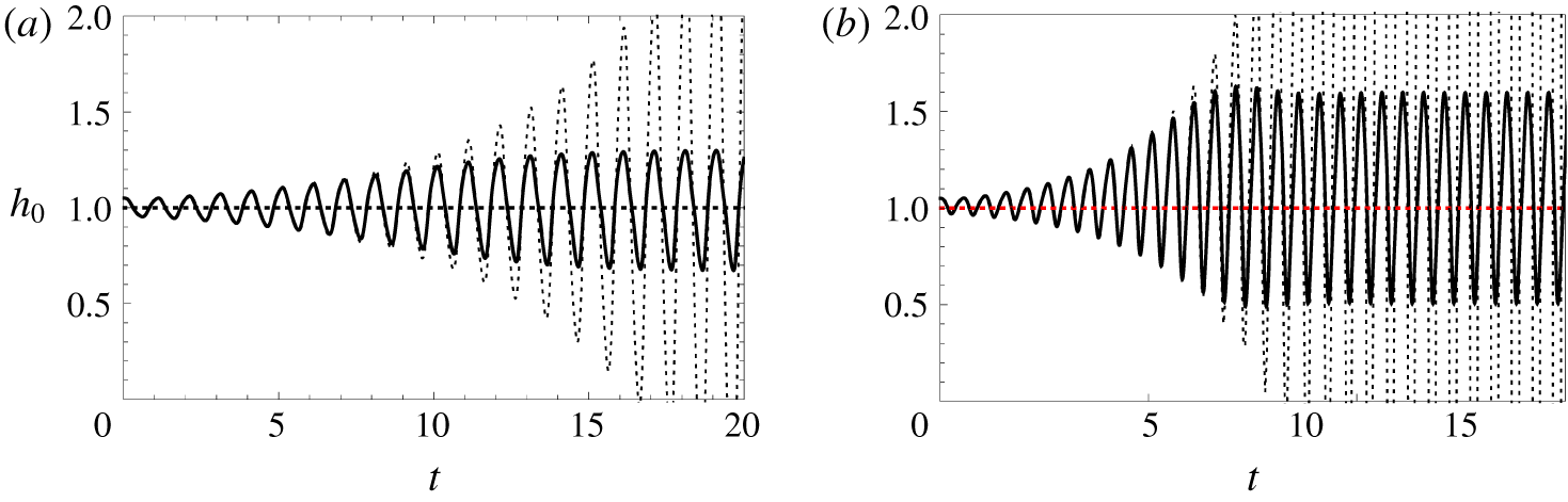
In figure 4(a)–4(b), the linear (dashed) and nonlinear (solid) responses corresponding to subharmonic and harmonic Faraday modes are plotted for the case of the pair of perfect dielectrics referred to in figure 2(a) (also cf. movie 1). It can be seen that the linear Mathieu response is oscillatory with an exponentially increasing amplitude and the nonlinear evolution of the interface agrees well with the Mathieu response for early times. From figure 4(a), it is evident that the SH response of the interface saturates nonlinearly to standing waves, isosynchronous with the forcing frequency. This is because the Maxwell stress at the interface has a quadratic dependence on the applied potential. Similarly, the harmonic response has a frequency twice that of the forcing frequency, as is evident from figure 4(b), and the interface oscillates twice every forcing cycle. The amplitude of the standing waves is found to increase with an increase in the forcing amplitude and the interface may approach either wall depending on the liquid–gas hold-up ratio.
Linear (dashed) and nonlinear (solid) temporal evolution of the interface position at  $x=0$,
 $h_{0}$, for the parameters corresponding to the markers in figure 2(a). (a) SH response at ●
 $(k=0.23,10.7~\text{kV})$. (b) Harmonic response at ▴
 $(k=0.42,13.1~\text{kV})$. Also cf. movie 1 for interface evolution.

The nonlinear response of a perfect conductor–perfect dielectric pair is very similar to that described above for a pair of perfect dielectrics and was discussed in an earlier work (cf. Pillai & Narayanan (Reference Pillai and Narayanan2018)). Similar responses are obtained for the case of a leaky dielectric model with fast relaxation times. The inertialess leaky dielectric model typically exhibits harmonic response at the onset of the instability. This type of inertialess harmonic response was also observed by Matar et al. (Reference Matar, Kumar and Craster2004) for a parametrically forced fluid with solutal dynamics at the interface.
4.2 Long-wave instability under steady forcing
We first discuss the linear stability results under the various limits of the LD model and then subsequently discuss the nonlinear dynamics of the interface. The wavenumber with maximum linear growth is obtained for the various limiting cases, as this is the perturbation used for nonlinear calculations.
4.2.1 Linear stability analysis
Pair of perfect dielectrics
The perfect dielectric model under steady forcing is described by (2.16a) and (3.5). Upon linearization, we get the linear growth rate,  $\unicode[STIX]{x1D6FC}$, as
 $$\begin{eqnarray}\unicode[STIX]{x1D6FC}=\frac{1}{3}\left[\frac{E\unicode[STIX]{x1D6FF}(\unicode[STIX]{x1D6FF}-1)^{2}k^{2}}{(1+\unicode[STIX]{x1D6FF}(\unicode[STIX]{x1D6FD}-1))^{3}}-\frac{1}{Ca}k^{4}\right],\quad \text{with }k_{max}=\sqrt{\frac{CaE\unicode[STIX]{x1D6FF}(\unicode[STIX]{x1D6FF}-1)^{2}k^{2}}{2(1+\unicode[STIX]{x1D6FF}(\unicode[STIX]{x1D6FD}-1))^{3}}}.\end{eqnarray}$$
In the above,  $k_{max}$ corresponds to the fastest growing wavenumber. This is used for nonlinear calculations in a later subsection. The expressions (4.7) were also obtained by Shankar & Sharma (Reference Shankar and Sharma2004) for the case of perfect dielectrics.
Perfect conductor–perfect dielectric pair
The limit of a perfectly conducting liquid is given by (2.16a) and (3.7), whence, upon linearization, we obtain the linear growth rate,  $\unicode[STIX]{x1D6FC}$, as
 $$\begin{eqnarray}\unicode[STIX]{x1D6FC}=\frac{1}{3}\left[\frac{Ek^{2}}{(\unicode[STIX]{x1D6FD}-1)^{3}}-\frac{1}{Ca}k^{4}\right],\quad \text{with }k_{max}=\sqrt{\frac{CaEk^{2}}{2(\unicode[STIX]{x1D6FD}-1)^{3}}}.\end{eqnarray}$$
Leaky dielectrics with fast relaxation time
The linear growth rate for the case of LD fluids in the limit of fast relaxation time is
 $$\begin{eqnarray}\displaystyle & & \displaystyle \displaystyle \unicode[STIX]{x1D6FC}=\frac{Ek^{2}}{(1+\unicode[STIX]{x1D70E}(\unicode[STIX]{x1D6FD}-1))^{3}}\left[\underbrace{\frac{\unicode[STIX]{x1D6FD}\unicode[STIX]{x1D70E}(\unicode[STIX]{x1D70E}-\unicode[STIX]{x1D6FF})}{2}}_{\mathit{Tangential~stress}}+\underbrace{\frac{(\unicode[STIX]{x1D70E}-1)(\unicode[STIX]{x1D70E}^{2}-\unicode[STIX]{x1D6FF})}{3}}_{\mathit{Normal~stress}}\right]-\frac{1}{3Ca}k^{4},\nonumber\end{eqnarray}$$
with
 $$\begin{eqnarray}\displaystyle k_{max}=\sqrt{\frac{3CaE\left[{\displaystyle \frac{\unicode[STIX]{x1D6FD}\unicode[STIX]{x1D70E}(\unicode[STIX]{x1D70E}-\unicode[STIX]{x1D6FF})}{2}}+{\displaystyle \frac{(\unicode[STIX]{x1D70E}-1)(\unicode[STIX]{x1D70E}^{2}-\unicode[STIX]{x1D6FF})}{3}}\right]}{2(1+\unicode[STIX]{x1D70E}(\unicode[STIX]{x1D6FD}-1))^{3}}}.\end{eqnarray}$$
Examining the expression for the linear growth rate,  $\unicode[STIX]{x1D6FC}$, in (4.9), it is evident that the normal stress due to the imposed electrical field is destabilizing when
 $\unicode[STIX]{x1D70E}>1$ and
 $\unicode[STIX]{x1D70E}>\unicode[STIX]{x1D6FF}^{1/2}$ as well as when
 $\unicode[STIX]{x1D70E}<1$ and
 $\unicode[STIX]{x1D70E}<\unicode[STIX]{x1D6FF}^{1/2}$. Identical conclusions of the destabilizing effect of the electrical field was shown to be true for a pair of leaky dielectrics with fast relaxation times in channel flow by Ozen et al. (Reference Ozen, Aubry, Papageorgiou and Petropoulos2006). They did so by solely examining the terms appearing in the linearized normal stress balance. However, from (4.9), it is important to note that the electrical field also affects the stability via the tangential component of the Maxwell stress. This effect of the electrical field, as is clearly evident from (4.9), is destabilizing when
 $\unicode[STIX]{x1D70E}>\unicode[STIX]{x1D6FF}$ and stabilizing when
 $\unicode[STIX]{x1D70E}<\unicode[STIX]{x1D6FF}$. It therefore follows that, in the
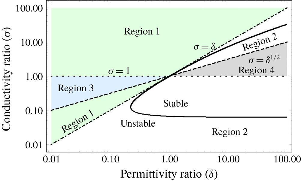
 $\unicode[STIX]{x1D6FF}{-}\unicode[STIX]{x1D70E}$ phase space, four distinct regions are obtained, demarcated by the three curves, viz.
 $\unicode[STIX]{x1D70E}=1$ (dotted),
 $\unicode[STIX]{x1D70E}=\unicode[STIX]{x1D6FF}$ (dot-dashed) and
 $\unicode[STIX]{x1D70E}=\unicode[STIX]{x1D6FF}^{1/2}$ (dashed), as shown in figure 5. In region 1, both normal and tangential components of the Maxwell stress are destabilizing. In region 2, the normal stress is destabilizing, while the tangential stress is stabilizing, whereas the opposite is true in region 3. Only region 4 corresponds to a zone where stability is guaranteed, wherein both effects of the electrical field are stabilizing. Ozen et al. (Reference Ozen, Aubry, Papageorgiou and Petropoulos2006) imply region 3 also to be stable, since their argument was based solely on examining the normal stress balance. However, region 3 and of course region 2 can become unstable depending on the relative magnitudes of the normal and the tangential components of the Maxwell stress. As an example, we show this to be true in figure 5, wherein the neutral curve (solid curve) is plotted for
 $\unicode[STIX]{x1D6FD}=10$. The last term in (4.9) due to capillarity is a stabilizing term and instability, i.e.
 $\unicode[STIX]{x1D6FC}>0$, is possible only when the two terms inside the square brackets due to the electric field is positive. The onset of instability is then obtained by equating the bracketed term to zero. Thus, we obtain the neutral curve in the
 $\unicode[STIX]{x1D6FF}-\unicode[STIX]{x1D70E}$ phase space as
 $$\begin{eqnarray}\unicode[STIX]{x1D6FF}=\frac{\unicode[STIX]{x1D70E}^{2}[3\unicode[STIX]{x1D6FD}+2(\unicode[STIX]{x1D70E}-1)]}{3\unicode[STIX]{x1D6FD}\unicode[STIX]{x1D70E}+2(\unicode[STIX]{x1D70E}-1)}.\end{eqnarray}$$
The above relation corresponds to a balance between the normal and tangential component of Maxwell stress. In the region enclosed by the solid curve, the net effect of electrical field has a stabilizing role for  $\unicode[STIX]{x1D6FD}=10$, while elsewhere it has a destabilizing role. It is clear that the region of destabilizing effect of the electrical field extends into all regions except region 4 (wherein the electrical field can only play a stabilizing role). Further, the maximum possible region of stability is obtained by taking the limit of
 $\unicode[STIX]{x1D6FD}\rightarrow \infty$ in (4.10), resulting in
 $\unicode[STIX]{x1D6FF}=\unicode[STIX]{x1D70E}$. Thus, the region of stability in the
 $\unicode[STIX]{x1D6FF}{-}\unicode[STIX]{x1D70E}$ phase space is always bounded from above by the
 $\unicode[STIX]{x1D70E}=\unicode[STIX]{x1D6FF}$ curve. In conclusion, regions 1 and 3 are always unstable, while region 4 is always stable. Parts of region 2 can become unstable depending on the electrical properties of the fluid pair as well as the fluid hold-up.
The effect of electrical field in the  $\unicode[STIX]{x1D6FF}{-}\unicode[STIX]{x1D70E}$ phase space, depicting the four regions demarcated by the three curves:
 $\unicode[STIX]{x1D70E}=1$ (dotted),
 $\unicode[STIX]{x1D70E}=\unicode[STIX]{x1D6FF}$ (dot-dashed),
 $\unicode[STIX]{x1D70E}=\unicode[STIX]{x1D6FF}^{1/2}$ (dashed). Normal component of the Maxwell stress is destabilizing only in regions 1 and 2. The tangential component of the Maxwell stress is destabilizing only in regions 1 and 3. In region 4, both components have a stabilizing effect. The heavy solid curve depicts the neutral stability curve for
 $\unicode[STIX]{x1D6FD}=10$. The region bounded by this curve is stable, while it is unstable elsewhere.

4.2.2 Nonlinear dynamics: sliding and cascading structures
We now discuss the nonlinear dynamics of the interface under steady forcing. Equation (3.8) along with (2.16a) is solved on a computational domain corresponding to one wavelength of the fastest growing wavenumber. The initial condition is  $h(x,0)=1+0.05\cos (kx)$ and
 $q(x,0)=0$. Here, the initial condition is chosen with the wavenumber corresponding to the fastest growing linear mode. This is because the fastest growing linear mode is expected to outgrow others and realize itself in experiments. Even if one of the other linear modes were to be chosen as the initial condition, the nonlinear interface evolution would exhibit qualitatively similar features. The number of grid points,
 $N$, is set to 500 for all calculations, as significant spatial resolution is required to obtain the shape of the interface as it approaches the wall.
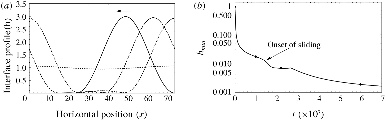
(a) Evolution of the interface between thin leaky dielectric films with  $\unicode[STIX]{x1D70E}=\unicode[STIX]{x1D6FF}$ (i.e. zero tangential stress) exhibiting spontaneous sliding;
 $t=0.001\times 10^{7}$ (dotted),
 $1\times 10^{7}$ (dot-dashed),
 $2.2\times 10^{7}$ (dashed)
 $6\times 10^{7}$ (solid). The arrow indicates the direction of horizontal translation. (b) The temporal evolution of the minimum position of the interface (
 $h_{min}$). Markers denote the time instant corresponding to the profiles in figure 6(a);
 $E=50$,
 $\unicode[STIX]{x1D6FD}=10$,
 $Ca=1$,
 $\unicode[STIX]{x1D6FF}=\unicode[STIX]{x1D70E}=2,k=0.085.$ Also cf. movie 2.

In this section, we discuss the long-time dynamics of the unstable interface. As anticipated from our earlier discussion, for the two cases of a pair of perfect dielectrics as well as a perfect conductor–perfect dielectric fluid pair, the interface dynamics is governed solely by the normal component of the Maxwell stress. It was already shown in an earlier work (Pillai & Narayanan Reference Pillai and Narayanan2018) that a perfect conductor–perfect dielectric pair exhibits sliding. We should anticipate this to be true also for the case of a pair of perfect dielectrics. In addition, the same is also true for a pair of leaky dielectrics with  $\unicode[STIX]{x1D70E}=\unicode[STIX]{x1D6FF}$, which corresponds to the case of zero interfacial charge and therefore zero shear stress due to the electrical field. The long-time dynamics of all these fluid pairs then resembles that of a Rayleigh–Taylor unstable interface. The interface evolution is depicted in figure 6(a) for a pair of leaky dielectrics with
 $\unicode[STIX]{x1D70E}=\unicode[STIX]{x1D6FF}$. The corresponding temporal evolution of the minimum position of the interface,
 $h_{min}$, is shown in figure 6(b). The markers in figure 6(b) denote the time instants of the interface profiles in figure 6(a). As can be seen (also cf. movie 2 for interface evolution), the initial primary trough evolves toward the bottom wall, driven by the normal Maxwell stress. The primary trough then slows down as it approaches the wall due to increased viscous resistance and undergoes capillarity-induced buckling, resulting in the formation of two secondary troughs. These secondary troughs continue to approach the bottom wall in a quasi-steady manner (at extremely slow rates), resulting in the formation of a large primary drop (called a ‘lobe’ by Lister et al. (Reference Lister, Morrison and Rallison2006a)), and a smaller satellite drop (called a ‘collar’ by Lister et al. (Reference Lister, Morrison and Rallison2006a)). At this point, the flow due to the Maxwell stress (
 $q|_{E^{n}}$) is negligible and the drainage is primarily driven by capillarity,
 $q|_{Ca}$. The fluid continues to drain from within the collar into the lobe and the interface evolves toward its final equilibrium configuration, as was shown by Yiantsios & Higgins (Reference Yiantsios and Higgins1989) and Lister et al. (Reference Lister, Rallison, King, Cummings and Jensen2006b). This equilibrium configuration corresponds to complete drainage of liquid from the collar into the lobe, resulting in a complete disappearance of the collar (i.e. the interface assumes zero thickness in this region) with the entire volume of fluid being confined within the lobe, which attains a width equal to
 $2\unicode[STIX]{x03C0}/k_{c}$. However, it is seen from figure 6(a) that the interface becomes unstable to asymmetric disturbances prior to reaching its equilibrium configuration at approximately
 $t\sim 1.5\times 10^{7}$ and undergoes horizontal translation, resulting in sliding. The phenomenon of sliding was conjectured to be an instability by Lister et al. (Reference Lister, Morrison and Rallison2006a) and was confirmed by the stability analysis of Dietze et al. (Reference Dietze, Picardo and Narayanan2018) using a frozen-time as well as non-modal stability analysis. As shown by Dietze et al. (Reference Dietze, Picardo and Narayanan2018), the sliding-induced asymmetric drainage of fluid from the collar into the lobe is energetically more favourable and helps to attain the equilibrium configuration faster, compared to a symmetric drainage of fluid through both secondary troughs.
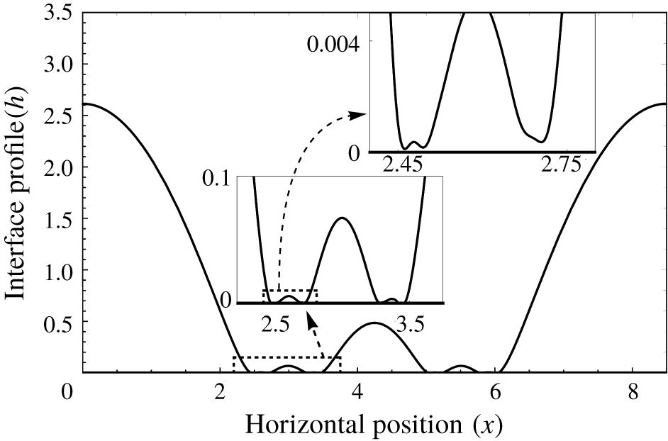
Long-time cascading structures exhibited by the interface for the case of zero normal stress (i.e.  $\unicode[STIX]{x1D6FF}=\unicode[STIX]{x1D70E}^{2}$) at
 $t=615$. The insets depict magnified view of the interface in the boxed regions near the wall;
 $E=50$,
 $\unicode[STIX]{x1D6FD}=10$,
 $Ca=1$,
 $\unicode[STIX]{x1D70E}=0.2$,
 $\unicode[STIX]{x1D6FF}=\unicode[STIX]{x1D70E}^{2}=0.04,k=0.74$. Also cf. movie 3.

Next, we look at the case of a pair of leaky dielectrics with  $\unicode[STIX]{x1D70E}=\unicode[STIX]{x1D6FF}^{1/2}$. This corresponds to the case where the interface experiences only tangential shear stress due to the electrical field, while the normal component of Maxwell stress vanishes. In this case, the instability mechanism is akin to that of the Marangoni instability. Figure 7 depicts the long-time interface profile corresponding to this case. As is evident, the interface does not exhibit sliding but instead undergoes a cascade of buckling events. The insets in figure 7 depict a magnified view of the interface configuration near the wall and a cascade of four buckling events is shown. As the surface charge density (
 $Q$) is slaved to the interface position (
 $h$), it also assumes similar profiles with time akin to the interface (not shown to avoid redundancy). Also cf. movie 3 for the spatio-temporal evolution of the interface. The video shows repeated events of buckling of the interfacial troughs as they approach the bottom wall. This behaviour is similar to the cascading structures observed in the long-wave thermal Marangoni instability (Boos & Thess Reference Boos and Thess1999). It is important to note that, unlike the earlier case discussed in the previous paragraph, no equilibrium configuration exists here. Instead, as the secondary troughs approach the wall, a competition between the capillarity-induced flow (
 $q|_{Ca}$) and the tangential Maxwell stress-induced flow (
 $q|_{E^{t}}$) in the draining thin film results in a point of divergence (i.e. a point with
 $q=0$) on the right of the left secondary trough as well as on the left of the right secondary trough. This draining mechanism is exactly identical to that discussed in detail by Dietze et al. (Reference Dietze, Picardo and Narayanan2018) for cascading structures observed in the case of thermal Marangoni instability. From this point, fluid is pulled toward either direction, subsequently producing tertiary troughs. These troughs grow until
 $q|_{E^{t}}$ increases again enough to compete with
 $q|_{Ca}$, resulting in further cascades. For a general leaky dielectric, the long-time dynamics is influenced by a combination of the normal and tangential components of the Maxwell stress, with the tangential stress dominating as the interface approaches the wall. This is because, as discussed earlier in § 2, the viscous resistance scales differently with the film thickness for the flow rate associated with the tangential and normal components of the Maxwell stress, with the former dominating the latter as the film thins. We show this to be true by taking the example of castor oil and
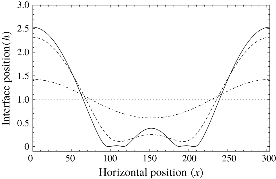
 $\text{SF}_{6}$ (Burcham & Saville Reference Burcham and Saville2000) in figure 8. It can be seen that, for this case as well, the interface exhibits cascading structures as it approaches the wall.
Spatio-temporal evolution of the interface exhibiting cascading structures for the case of castor oil and  $\text{SF}_{6}$ (Burcham & Saville Reference Burcham and Saville2000);
 $\unicode[STIX]{x1D6FD}=10$,
 $k=0.01$.

5 Summary
An inertial lubrication model is developed to track the nonlinear evolution of an interface between a pair of leaky dielectrics, subject to normal electrostatic forcing. Cases of both periodic as well as steady forcing are investigated. The former case focuses on resonant instability in thin inertial LD films, while the emphasis in the latter is on the long-time dynamics of the interface prior to rupture.
For AC electrostatic forcing, in the two limits of a perfect conductor–perfect dielectric pair as well as a pair of perfect dielectrics, the system becomes unstable only to an inertial resonant instability, leading to subharmonic or harmonic response of the interface. For a general pair of leaky dielectrics, an inertialess resonance can occur due to charge dynamics at the interface, wherein the interface response is reminiscent of a highly damped system and typically exhibits harmonic response. While the result of the two limiting cases requiring mechanical inertia for resonance is expected, the general result of the LD model not requiring mechanical inertia is reminiscent of models with an insoluble surfactant at the interface. Therefore, in LD films, one can observe a smooth transition from an inertialess resonance due to charge capacitance to an inertial resonance due to mechanical inertia of the fluid.
For DC electrostatic forcing, the regions corresponding to the stabilizing and destabilizing effects of the electrical field in the  $\unicode[STIX]{x1D6FF}{-}\unicode[STIX]{x1D70E}$ phase space are obtained in the limit of fast relaxation time. It is shown that, when the interface evolution is dominated by the normal component of Maxwell stress, the long-time dynamics exhibits sliding akin to Rayleigh–Taylor instability, wherein the interface translates parallel to the wall. This happens in the case of a perfect conductor–perfect dielectric fluid pair as well as a pair of perfect dielectrics. The onset of sliding is prevented in a general leaky dielectric fluid pair on account of the presence of the tangential component of the Maxwell stress, which is set into effect by the presence of interfacial charge. The interface dominated by the tangential component of the Maxwell stress exhibits cascading structures akin to the long-wave Marangoni instability.
Acknowledgements
We acknowledge financial support from NASA (NNX17AL27G).
Declaration of interests
The authors report no conflict of interest.
Supplementary movies
Supplementary movies are available at https://doi.org/10.1017/jfm.2020.112.