



No CrossRef data available.
THE OBSIDIAN BLADE SEQUENCE AT EL UJUXTE, A LATE PRECLASSIC SITE ON THE SOUTH COAST OF GUATEMALA
Published online by Cambridge University Press: 28 March 2006
Abstract
Systematic data on about 1,200 blades from this site were summarized in terms of three ceramic phases (defined by Love 2002b) for the same site. That is, we assigned blades to phases based on the ceramic content of each provenience. Regular phase-by-phase decreases occurred in blade dimensions, weights, and length-to-width ratios. We predicted these results based on earlier findings from the site of La Blanca (Nance and Kirk 1991). The trend appears also within the latest Pitahaya phase, even at the level of the excavation unit. Blade densities decrease through Pitahaya deposits, as well, and the blade sequence is discussed in terms of an increased scarcity of obsidian or obsidian blades traded to the region.
Information
- Type
- Research Article
- Information
- Copyright
- © 2005 Cambridge University Press
In earlier research at the Middle Preclassic site of La Blanca on Guatemala's southern coast and now at the nearby Middle to Late Preclassic site of El Ujuxte (Figure 1), we have documented a gradual decrease in prismatic blade size through time. Much of the real cost of blades to these people would have been in transporting blade-quality obsidian from the Guatemalan Highlands (see Tabares et al. 2005 on El Ujuxte obsidian sources). Gradually learning to cope with smaller blade-tool bits might have lowered the cost per blade to El Ujuxte importers. Human porters could have transported more small blades per load, more small cores versus larger ones, and so on. So, one possible explanation for the decrease in blade size at these sites is increased efficiency on the part of consumers. If, however, smaller blade size was dictated by suppliers in either the highlands or elsewhere on the southern coast and not recipients at El Ujuxte, then we might be looking at the problem of interrupted trade and obsidian-blade scarcity.

Regional map with key sites.
While there are many difficulties surrounding the study of blades, the technique used here was to create a computerized dataset, a matrix in which each data line contained information about an individual blade, and each column contained information about a variable describing the blades or their provenience in the site. Variables systematically recorded have to do with blade morphology, aspects of edge wear, edge alteration, and blade size. For the purposes of this research, the term blade refers to either a complete prismatic blade or a blade section created when a blade is snapped across its longitudinal axis. Blade fragments without complete cross-sections were excluded from the dataset.
It is important to state at the outset that this is not a study of the technology of blade production. The authors never examined all of the obsidian from El Ujuxte but were sent about 3,700 catalogued specimens of blades and possible blades chosen by laboratory personnel. From these, we selected 1,260 blades according to criteria stated earlier.
In earlier research, C. Roger Nance and Katharine Kirk (1991) proposed a sequence of changing obsidian-blade complexes for the Middle Preclassic site of La Blanca on the southern coast of Guatemala. That study was based on samples of blades from four different portions of the site ceramic sequence. Michael Love (2002a) excavated La Blanca and also defined the ceramic sequence there.
We found that through time, obsidian blades from La Blanca gradually decreased in size in terms of decreasing lengths, widths, and thicknesses, as well as weights. Blade proportions changed, with length-to-width ratios becoming progressively smaller. Edge wear increased on the lateral edges of blades through the sequence, and resharpening of blades became more common, as shown by increased bipolar modification, which served to renew lateral blade edges. All of this suggested an increasing scarcity of obsidian for the inhabitants of La Blanca.
As for La Blanca, the El Ujuxte obsidian study followed that for ceramics, and ceramic-phase designations were used to determine relative chronological positions for obsidian samples (collected by excavation unit and 10 cm level). Also consistent with the La Blanca research, all pieces of obsidian were collected systematically by screening deposits through one-eighth-inch hardware cloth.
Love also excavated El Ujuxte and recently described the site ceramic sequence, dividing it into three phases. They fall into the later portion of the Middle Preclassic (Caramelo phase) and the Late Preclassic (Cataluña and Pitahaya phases). All together, occupation at El Ujuxte spans the period of about 540 b.c. to sometime after a.d. 100 (Love 2002b).
PHASE BY PHASE TRENDS AT EL UJUXTE
Once El Ujuxte blades had been assigned to these phases, we could see that blade-sample size varied widely among the three phases. Of 1,260 blades in the study, only 10 are from the earliest, Caramelo phase; 37 are from the Cataluña phase. This leaves the preponderance of blades—1,213, or 96.3%—in the latest, Pitahaya phase.
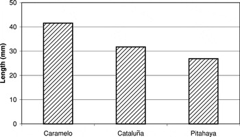
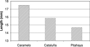
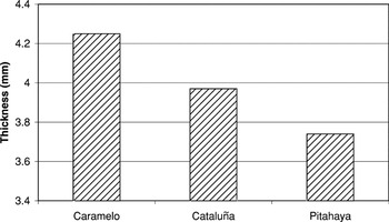
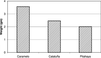
Notwithstanding this skewed distribution of blades across the three phases, there are consistent trends in the data of Figures 2, 3, 4, and 5. In all four bar charts, mean dimensions and weights decrease regularly through time from phase to phase, with changes in lengths and weights being more pronounced than those in widths and thicknesses.

Mean length by phase.

Mean width by phase.

Mean thickness by phase.

Mean weight by phase.
Are differences among the phases for these four size variables collectively significant? While t-tests could be used to test significance for each pair of means, the problem with separate t-tests is that results are presented as independent outcomes, while clearly they are not. So if we find weight to be different and length to be different, we are really presenting the same result twice if length and weight are highly correlated. To explain the chi-square test employed, we have to remember two things. First, the chi-square distribution with p degrees of freedom is the distribution of the sum of squares of p standard normal variables. Second, the central limit theorem says that under very general conditions, averages (means) are approximately normally distributed. We apply this in the following way. Figures 2, 3, 4, and 5 show one set of means for each phase. These means will be approximately normally distributed, which means that the difference between the rows will be approximately normal, as well. To compute the chi-square, we cannot simply take the sum of squares of the differences between rows, because columns (variables) are not independent. Length, weight, and so on are (pretty strongly) correlated. We use the actual correlations to weight the sum of squares of four correlated normal random variables in such a way that it becomes approximately the sum of squares of four independent normals—that is, it becomes approximately chi-square distributed. Testing the hypothesis that the rows of means are equal, and taking the correlation of variables into account, between the Pitahaya phase and the Cataluña phase, the chi-square is 7.61, with P < .04; between the Cataluña phase and the Caramelo phase, the chi-square is 5.74, with P < .08; and between the Pitahaya phase and the Caramelo phase, the chi-square is 16.03, significant at p < .001.
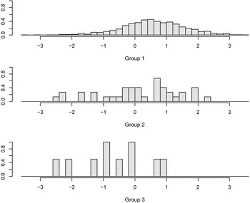
Another way of approaching the same problem is with a discriminant analysis (Figure 6). Here we make a weighted sum of the four variables in such a way that (a) the weighted sum has variance one; and (b) the means of the three groups (phases) are as far apart as possible. Thus, we maximize the between-group variance relative to the total variance. It turns out that the weighted sum (linear combination) we make accounts for 95% of the between-group variance—that is, there is effectively only one dimension (size) in which the three groups differ. Figure 6 shows the distribution of blades in terms of this new “size” variable for the three phases, with “smallness” represented by positive values to the right and “largeness” by negative values to the left. One can see an increasing shift from large blades in the earliest group (group 3, or Caramelo phase) to small blades in group 1 of the Pitahaya phase.

Discriminant analysis.
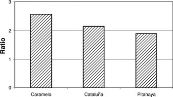
Also, mean length-to-width ratios decrease regularly (Figure 7). In sum, blades gradually become both smaller and squarer through time. Given the earlier research at La Blanca, these regular trends of both decreasing blade size and changing proportions had been hypothesized. And so we find a parallel trend and statistical support for the idea that there is some tendency on the southern coast during Preclassic times for blades gradually to become smaller and squarer through the sequence.

Mean length:width ratio by phase.
TRENDS WITHIN THE PITAHAYA PHASE
If this were a pervasive trend, then it seemed predictable that similar shifts would be found not just from phase to phase but also continuing through El Ujuxte deposits of the Pitahaya phase, which produced 96% of all blades in the study.
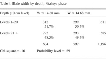
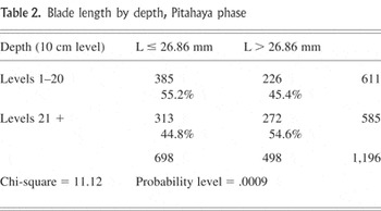
We focused, then, on a large Pitahaya subset of 1,196 blades. These came from 12 excavation units with deep deposits, averaging about 3.0 m per 2 × 2 m square, and we divided the levels arbitrarily into those above and below 2 m. This produced two large, roughly equal samples of blades, 611 above 2 m (levels 1–20), and 585 below. Much larger Pitahaya samples allowed direct use of the chi-square test, so for dimensions, weights, and length-to-width ratios, we used means to divide the blades into large and small fractions. Along with cross-cutting sampling from upper and lower deposits, this resulted in two-way, four-cell tables. Blade thicknesses and widths (Table 1) vary little by macro-level when viewed in this way. However, lengths decrease significantly from lower to upper Pitahaya deposits (Table 2), as do weights and length-to-width ratios. These trends parallel findings described earlier among the three El Ujuxte phases.
Blade width by depth, Pitahaya phase

Blade length by depth, Pitahaya phase

CORRESPONDENCE ANALYSIS: DISTRIBUTION OF SAMPLES
Although these trends are significant statistically, they are a bit suspect, since blades can sometimes occur concentrated in large quantities. Several large deposits of blades representing different tasks could produce an apparent sequence with little if anything to do with gradual cultural change. There is reason, then, to search for evidence of a pervasive trend within individual excavation units that produced Pitahaya-phase material. This was accomplished through a statistical technique known as correspondence analysis (Greenacre and Blasius 1994). Archaeologists occasionally have employed correspondence analysis in their research (e.g., Bølviken et al. 1982; Clouse 1999); the authors (Nance et al. 2003) recently used this technique in a study of ceramics from Iximché.
Working with the same large Pitahaya subset, we made a summary dataset with information about 31 samples of blades, each sample coming from a group of contiguous 10 cm levels of a single excavation unit. The idea was to maximize sample size and still preserve evidence of stratigraphic change. The average sample contained data on 36 blades and represented between 11 and 12 levels of an individual unit. This summary dataset contained information not only on dimensions and weights, but also on edge wear, blade modification, and other variables, including blade proportions relative to available debitage, which we had also summarized. It did not, however, contain information on provenience. That is, level and unit designations were not incorporated.
In a correspondence analysis, distances among samples are computed using chi-square statistics. One can imagine three samples and three chi-square tests contrasting each sample to the other two. For a study of, say, five variables, each test would involve a ten-cell contingency table. The results for three samples could be represented on a two-dimensional grid. Sample loci close together on the grid would resemble one another in variable frequency proportions, since the distance between them would represent a small chi-square value. With many samples, the procedure is the same, except that it is impossible to conceptualize visually the multiplicity of relationships. The correspondence-analysis statistic, however, reduces all of the chi-square distances among all the samples onto a two-dimensional grid in what can be considered a best possible fit.
The same analysis also computes chi-square distances among the variables. In the earlier example, for three samples and five variables, we would generate 10 chi-square tests, each for a 6 cell contingency table, contrasting the frequencies for two variables as distributed within three samples. Both sample and variable loci can be depicted on the same plot (or joint plot). Variable loci situated near each other have similar distributions among the samples, and variable loci are situated near samples where they are highly represented.
In the study at hand, we generated a single correspondence analysis for 31 samples and 16 variables (represented by 46 constituent attributes), so the resulting joint plot contains 77 labeled points or loci. To see the results with some clarity, however, only selected loci are depicted in three figures (Figures 8, 9, 11), all taken from the same analysis.
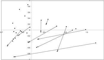
Figure 8 shows all 31 samples projected on a two-dimensional plot. Also in Figure 8, samples from nine of the individual units are shown connected with a line, the arrow pointing from the upper to the lower sample. Based on stratigraphic evidence, then, there is a time line running through the chart from upper right to lower left. This trend is evident for nine of the 12 squares represented in the analysis. In short, there is evidence of a blade sequence running through the 200 years of Pitahaya occupation.

Correspondence analysis, sample loci.
CORRESPONDENCE ANALYSIS: DISTRIBUTION OF VARIABLES
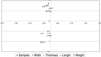
Figure 9 depicts sample loci for only excavation Unit 17-2, the three samples isolated in the upper left-hand corner of Figure 8. The three samples for this unit do not line up chronologically—that is, diagonally across the plot—as do those for the nine units shown in Figure 8. Also included in Figure 9 are loci for four of the 16 variables that figured in the analysis. These have to do with size: length, width, thickness, and weight. The constituent attributes of each variable are plotted, and each of these summarizes frequencies of blades with above- and below-average measurements for the size variable in question. In other words, on the chart, each size variable is represented by two attributes. It so happens that for all four variables, the attribute locus having the higher Y value on the chart represents the smaller size attribute, and the lower Y value represents the larger. For example, the width variable is summarized through two attributes: below-average width and above-average width. The attribute above-average width is represented by an X below the Y = −.5 grid line in Figure 9. The locus for below-average width is represented by an X above the Y = .5 grid line.

Correspondence analysis, variable loci.
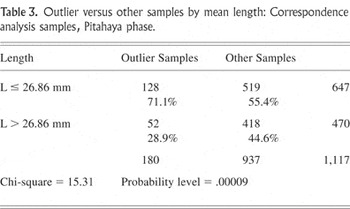
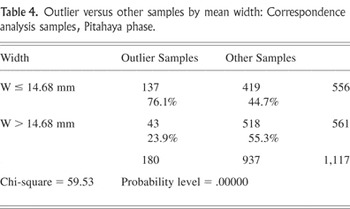
These data in Figure 9 allow us to examine the other perspective of Pitahaya blade distributions—horizontal rather than vertical and synchronic rather than diachronic. Can we discern subassemblages that might reflect differing patterns of blade use across the site? Given that the positions of the three sample loci of Unit 17-2 are in close proximity to all four below-average size attributes (Figure 9), we would anticipate that the 180 blades from these samples, combined, would be quite small compared with blades from the 28 other Pitihaya samples. This turns out to be the case. Not only are lengths (Table 3) and weights lower for these “outlier” samples; but widths (Table 4) and thicknesses are lower, as well, and these differences are highly significant. We do not seem to be dealing here simply with a late portion of the sequence—for example, length-to-width ratios vary little when comparing these two groups of samples. The excavation unit in question was situated in a level area near the bases of two mounds (Mounds 36 and 38), possibly where trash was dumped or accumulated (Love, personal communication 2004). For some reason, those working at this locality required and obtained delicate blades produced from small cores.
Outlier versus other samples by mean length: Correspondence analysis samples, Pitahaya phase.

Outlier versus other samples by mean width: Correspondence analysis samples, Pitahaya phase.

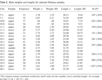
It can be seen in Figure 9 that the weight-dimension attributes cluster in four pairs: weight + (i.e., above average) and length +; weight − and length −; thick + and width +; and thick − and width −. In other words, blade length co-varies closely with weight among the samples, and blade width co-varies with thickness. In Figure 8, the nine line segments, each representing a different excavation unit, all have positive slopes, and such would be the case for a line segment approximately connecting the pairs weight +, length + to weight −, length −. This positive diagonal represents time to some extent, and we know that blade lengths (Table 2) and weights become smaller through the Pitahaya phase. In contradistinction, a line segment connecting thick +, width + to thick −, width − would have a negative slope, and there is no clear evidence that blade width (Table 1) or thickness changes appreciably through Pitahaya levels. Of course, one can see two general clusters, as well—small blade dimensions and weights, on the one hand, and large dimensions and weights, on the other—separated along the Y axis. As discussed earlier for interphase differences, all size variables tend to co-vary. However, based on available Pitahaya evidence, it seems that lengths and weights have more to do with time, and widths and thickness have more to do with functional variability across the site. Table 5 summarizes, by Pitahaya sample, lengths (in mm) and weights (in grams) for the nine excavation units with aligned samples in Figure 8. In terms of these dimensions, average blade size generally decreases within these units from lower to upper samples. At the same time, standard deviations in Table 5 are large, indicating size diversity within samples; sample size in most cases is small. Due to the problem of sampling error, this trend does not show up well within individual units on a level-by-level basis. For example, Pearson's correlation coefficients comparing blade lengths and level assignments for each unit (Table 5) are only statistically significant (P < .05) for three of the four excavation units producing at least 50 Pitahaya blades and for none of the other units represented in the table.
Blade weights and lengths for selected Pitahaya samples.

USE WEAR AND BLADE SIZE
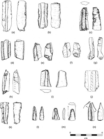
Other variable loci in the correspondence analysis figure in this research. Not yet considered is the idea that decreasing blade size through time might have been due to increased modification (retouch) or edge wear. For example, it is certainly plausible that if the incidence of bipolar flaking had increased, this could have caused blade size generally to diminish. However, bipolarly flaked blades, while common enough in the collection (Figure 10e–h), did not increase through the Pitahaya sequence. Proportions of these modified blades actually decrease slightly from 5.5% of blades below level 20 to 4.1% in levels 20 and above. In terms of dimensions and within the same Pitahaya sample, bipolarly flaked blades are significantly below average in width but significantly above average in thickness. It seems likely that thin blades would not have stood up to the percussion-flaking of the bipolar technique.

Blade illustrations.
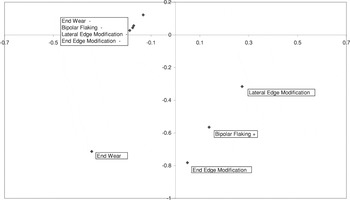
Figure 11 shows variable loci in the same correspondence analysis having to do with deliberate edge modification: on blade ends (e.g., burins; Figure 10i–j); through bipolar flaking; and on lateral edges (Figure 10k). One other variable included in Figure 11 summarizes edge alteration interpreted to be the result of use—in this case, wear on blade ends (e.g., drill bits; Figure 10l–n). These four variables are each expressed in terms of two attributes, one summarizing frequencies of blades with, versus one for those without, one of these forms of (interpreted) deliberate modification or incidental edge use wear. Figure 11 shows that attribute loci for these variables where evidence for wear or modification was absent (indicated by a minus sign) cluster together in the upper left corner of the chart and are situated near the small blade-size attributes (cf., Figures 9 and 11). The positive attribute loci for these same variables are located below and to the right. The correspondence analysis, then, does not suggest a tendency for blades of small size and those manifesting one or more of these forms of edge alteration to cluster on a sample-by-sample basis, or, likewise, that these attributes tend to be represented together on the same blades.

Correspondence analysis, other variable loci.
As interpreted here, the most pervasive form of edge wear from use on El Ujuxte blades consists of very fine pressure flaking along blade lateral edges (Figure 10a–d). We found that blades showing this form of use wear, instead of being diminished in size, are actually significantly larger in all dimensions compared with those lacking this lateral edge alteration. All together, blades showing marked lateral edge use tend to be large and seem better suited for heavy tasks (cf. Nance and Kirk 1991).
Also, this general form of lateral edge wear does not become more pronounced on blades above level 21 of the Pitahaya sample. Actually, there is a slight though statistically insignificant tendency for pronounced edge wear to occur on Pitahaya blades more frequently in lower levels.
In sum, there is no clear evidence that diminished blade size in upper Pitahaya levels was due either to more intensive use or to an increase in deliberate modification.
DISCUSSION
Blade densities fall off significantly in the upper levels of Pitahaya deposits (Figure 12). While this could be due to a late increase in building activity, viewed in conjunction with decreasing blade sizes the finding is noteworthy and could suggest a declining blade industry at El Ujuxte. Also, blades changed in terms of their shape, becoming more square-like, as they declined in overall size. Cores producing the blades might have become shorter, since blade midsection to end-section proportions changed little (Figure 13). Apparently, blade length did not decrease, because blades were being snapped into more and shorter sections. All together, then, the picture suggested is one of both fewer and smaller blades being manufactured at El Ujuxte and/or arriving there during the later stages of the Pitahaya occupation. The more squared shape of the later blade sections might have functioned to maintain the strength of these smaller tool bits and to prevent them from shattering during use.

Pitahaya blade density by level.

Blade morphology percentages by level.
While the fall off in blade density through the deposits and the decreasing blade size both indicate an increasing scarcity of blades at El Ujuxte, this deprivation might have been felt unevenly across the prehistoric community. In one of the field reports, Love and colleagues (1997) identified a structure at El Ujuxte (Mound 46) as possibly an elite residence. Love excavated two units there, and blades from those pits (18-1, 18-2) are included in this research. Looking at level-to-level trends in these two units, blades do become smaller through time (significantly so, as measured through the correlation coefficient; see Table 5), but when elite blades are contrasted to those from other Pitahaya samples, those from this potentially elite locality are larger in all size variables, most significantly in terms of weight (Table 6).
Elite versus other samples by mean weight: Correspondence analysis samples, Pitahaya phase.

Robert Santley (1989:143) studied obsidian from Matacapan and surrounding sites in the Tuxtla Mountains of Veracruz, reporting that obsidian blades “from the center of Matacapan exhibit less utilization than blades from outlying areas of lower status occupation indicating that elites were more affluent consumers of obsidian.” He was suggesting that, given their abundant supply, elites discarded blades before they became highly worn. This correspondence, however, might not hold for some prehistoric Mesoamerican communities, where there was an overall scarcity of blades. At El Ujuxte for the same Pitahaya samples under discussion, we found significantly more edge wear on blades from the potentially elite context, not less.
In both the El Ujuxte and La Blanca studies, we classified and recorded lateral edge wear, using low-power microscopy and following Hay (1978) in terms of three categories: (1) wear minor to absent, often shown as discontinuous edge nicking; (2) moderate, definite wear in the form of minute, contiguous pressure-flake scars, at times forming a bevel surface running parallel to the edge but less than 2 mm wide; and (3) heavy edge wear with bevel surfaces equal to or wider than 2 mm. In Table 7, blades are represented by composite scores that include data for both lateral edges (i.e., we added attribute codes together for each blade). A minimum score, then, would be 2, and a maximum would be 6. Only blades with both edges classified in the 1–3 range are included (leaving out the relatively few blades with other forms of lateral edge wear; e.g., ground edges). As can be seen, a high proportion of elite blades have scores of 5 or 6, while blades from contexts not identified as elite tend more to fall in the category for the lowest composite score. It would appear that elites, with larger blades at their disposal, were able to employ these tools for a more complete range of activities, including forceful use of tools bits. If their supplies of blades were more abundant, dulling tool edges in the performance of these tasks might have been less a matter of concern than for others with more restricted access.
Elite versus other samples by composite lateral edge wear scores: Correspondence analysis samples, Pitahaya phase.

EXTRA-SITE COMPARISONS
Detailed comparisons of La Blanca and El Ujuxte data do not reveal a regular sequence from large to small blades when samples from the two sites are interdigitated chronologically. However, there are size decreases at each site. This lack of consistency may be due to small sample sizes and sampling error or possibly, to local histories that may or may not be individual expressions of a regional trend. John Clark (1988:46) reported for the Middle Preclassic site of La Libertad in the central depression of Chiapas a trend “away from a specialized blade industry towards an industry of expediency.” At all three sites, then, during Late or Middle Preclassic times, we see evidence of a deteriorating blade industry.
Another area of comparability has to do with access to blades by people of high rank versus commoners. Clark (1987:280–281), in an assessment of excavated Middle Preclassic sites in highland Chiapas, saw blades as status markers in those communities, with most blades belonging to high-status individuals. Also, investigators working in Vera Cruz have found high concentrations of obsidian or obsidian blades in site centers or ceremonial or elite contexts (Barrett 2003:216; Knight 1999:176–179; Santley 1989:143). Certainly, these observations are compatible with our findings for the Late Preclassic at El Ujuxte. As indicated earlier, the possibly elite residence, Mound 46, produced larger blades than other contexts.
Earlier, we noted that diminished blade size can be viewed as either a positive or a negative development for prehistoric populations. In Europe, blade size appears to decrease regularly through the Upper Paleolithic (Owen 1988:157–158), presumably resulting in the microliths of Mesolithic and Neolithic times. While this could represent a worldwide trend toward smaller, lighter, more efficient tools, we can ask why it shows up so clearly through just 200 years of Maya prehistory.
Laura Kosakowsky et al. (1999) identified extensive trade in Fine Red pottery from the coastal plain of southeastern Guatemala into the adjacent highlands and suggest a contrasting “flow of obsidian” from the highlands in exchange. In their interpretation, this “exchange of finished products … becomes institutionalized in the Classic period,” trade that had “become formalized by well established trading relations now dating back to the Late Preclassic” (Kosakowsky et al. 1999:388). Our own research with obsidian from two sites on the northwest southern coast of Guatemala and that of Clark (1988) at La Libertad in Chiapas suggest more tenuous trade in highland Guatemalan obsidian to surrounding regions during the Middle to Late Preclassic period.
CONCLUSIONS
As Kenneth Hirth and Bradford Andrews (2002:1) note in their introduction to Pathways to Prismatic Blades, Mesoamerican researchers in recent decades have taken a technological approach to the study of lithic artifacts and have tended not to deal with the morphology or function of finished stone tools. This approach has yielded valuable results, but it does not preclude the efficacy of studying the finished product. Also, it is not so much that this is a comprehensive development in Mesoamerican lithic archaeology but that recent research has by and large focused on obsidian prismatic blade industries. For sites where lithic assemblages are not dominated by prismatic blades and debris from their manufacture and use, both for Mesoamerica and elsewhere in North America, lithic studies routinely involve consideration of both technology of production and the morphology and function of finished tools. The difference here seems to lie in the importance of classification to the research enterprise. Hirth and Andrews (2002:1) write that “the lithic technology approach … provides a useful heuristic framework for classifying lithic artifacts.” Generally, archaeologists involved with prismatic blade industries classify various forms of debitage from core and blade manufacture, the cores themselves, and the resultant blades. Yet the preponderance of finished tools, the prismatic blades, are rarely if ever broken down into subcategories with demonstrable analytic value, except those based on parent material. This suggests that finished prismatic blades have not been susceptible to classification. To some extent, this may explain the heavy emphasis on the technology of blade production in recent Mesoamerican research. For non-blade assemblages, of course, finished stone tools tend to classify into known types of projectile points and other chipped- and ground-stone tool forms.
As perceived here, the problem of classifying blades can be avoided through a multivariate approach, and prismatic blades can then be studied as one of several research components, including production technology, in the overall assessment of a site's obsidian assemblage. For the sites of La Blanca and El Ujuxte, this extra-blade research remains incomplete and, as a result, important questions remain unanswered. Debitage and other non-blade obsidian from El Ujuxte should be examined to ascertain whether blades were manufactured there. A. Natasha Tabares and colleagues (2005) mention, apart from blades, the presence at El Ujuxte of obsidian “flakes and casual tools.” Did these artifacts also decline in density through the Pitahaya deposits along with blades? Another possibility is that they became more important relative to blades in later years of the Pitahaya occupation, paralleling Clark's (1988) findings at El Libertad. Finally, it is possible that some shift in production technology at El Ujuxte or elsewhere to some extent accounts for the diminution of blade size. This question can and should be explored, as well.
Yet if our research at these two sites is incomplete, is this not also the case elsewhere, where thousands of blades simply have been subsumed within one or several categories without further discussion? One should keep in mind that each of these blades, for the most part, is a complete tool bit, and that the research potential for these thousands of artifacts must be considerable. At least, this is suggested by our research at La Blanca and El Ujuxte.
We found that blades in Mesoamerica can change in measurable and statistically significant ways, and that this can occur within surprisingly limited time frames (e.g., over the 200-year period of the Pitahaya phase).
That these trends appeared consistently through most of the excavation units studied contributes to an understanding of the depositional history of the site. Our data support the idea that Pitahaya deposits built up gradually and generally did not result from a one-time, massive construction project.
Our research underscores the fact that technological issues surrounding blades do not end with their production. Artisans routinely modified blades to create specialized tool bits and recycled them as edges became worn. The size and shape of tool bits, their modification, and the degree and nature of edge wear relate not only to function but also, evidently, to the availability of obsidian.
This study also points to the potential role of blade research in the study of intrasite settlement patterns. For El Ujuxte, this is a work in progress for Love and his collaborators. Some unique cultural context might be found for the concentration of small blades in the vicinity of Mounds 36 and 38, and the overall pattern might be found replicated on other areas of the site. The definition of sociopolitical boundaries at El Ujuxte might be enhanced through further blade studies if elite habitations are consistently found to be marked by high proportions of large blades.
Finally, our research indicates not only that one can study trade routes and sources of raw material through trace element analysis, but also that, through the study of blades and other obsidian tools and debitage, the potential exists to study both the development and decline of this trade, as well.
RESUMEN
Se resumió los datos obtenidos sistemáticamente de aproximadamente 1,200 navajas de obsidiana procedentes del sitio El Ujuxte, ubicado cerca de la costa sur de Guatemala, de acuerdo a tres fases cerámicas que Michael Love definió en 2002 para dicho sitio. Es decir, asignamos navajas a las fases con base en el contenido cerámico del contexto en el cual se les descubrió. Se detectó que de fase en fase occurió disminuciones en las dimensiones de las navajas, en los pesos y en las proporciones de largo:ancho. Nosotros habíamos predicho estos resultados al tomar como base los descubrimientos anteriores que realizamos en el sitio La Blanca (Nance y Kirk 1991).
La mayoría de las navajas de El Ujuxte se deviaron de la fase Pitahaya del preclásico tardio. Y aún dentro de sus 200 años de trayectoria, las navajas muestran un cambio notable hacia tamaños más pequeños, medidos en términos de largo y ancho. Esto puede observarse en 9 de las 12 unidades de excavación con buenas muestras de navajas (Cuadro 1). También, encontramos variabilidad a lo largo del sitio durante la ocupación Pitahaya, como aparece en el análisis de las pruebas estadisticas de correspondencia. Una de las unidades de excavación produjo navajas particularmente pequeñas, que no sólo disminuyeron en longitud y peso sino que también tuvieron anchos y grosores menores. En un área del sitio, que fue identificada como una residencia de elite se encontró navajas significativamente más largas que las otras encontradas en el resto del sitio durante le ocupación Pitahaya.
Asimismo, registramos sistemáticamente la evidencia de las huellas de uso y las modificaciones de retoques en estas navajas, y pudimos determinar que los cambios en los tamaños de las navajas no fueron resultado de estos factores. También, al estudiar la morfología de las navajas, determinamos que el cambio en la longitud de las navajas no fue determinada por quebrarlas para producir más herramientas que fueran más cortas. Las densidades de navajas decaen en los depósitos superiores de la fase Pitahaya, y la explicación más probable para todas estas tendencias es que tanto las navajas como la obsidiana fueron cada vez más escasas para los habitantes de El Ujuxte.
ACKNOWLEDGMENTS
Investigations at El Ujuxte were carried out with the permission and cooperation of the Instituto de Antropologia e Historia de Guatemala. We thank the Departamento de Prehipánicos y Coloniales and its personnel for facilitating the project. Research at El Ujuxte was funded by the following sources: the John H. Heinz III Foundations, the Wenner-Gren Foundation (Grants 6548 and 5837), a Fulbright-Hayes Fellowship, the National Science Foundation (SBR-9510991, SBR-96171123, and SBR-9807304), the Foundation for the Advancement of Mesoamerican Studies, the Universidad del Valle de Guatemala, Sonoma State University, and California State University, Northridge. Additionally, and specific to the research reported here, the authors would like to thank Michael Love for his insights and the cooperation he provided throughout the project. We are grateful to the Ancient Mesoamerica reviewers, John Clark, Jay Johnson, and an anonymous reviewer who provided helpful criticisms. Marvin Jeter helped in this regard as well. Thanks are also due to Alice Burns for her drawings of the blades, to Sandra Wong for preparing Figures 1 and 10, and to Matilde Ivic for translating the Spanish-language resume. The late Clyde Nance, the senior author's mother, volunteered many hours, typing the data into the computer and later, assisted by Kathy Prado, checking for entry errors. Her assistance here and in other projects over the years is gratefully acknowledged as well.
References
REFERENCES
Barrett, Thomas P.
2003
Tuxtlas Obsidian: Organization and Change in a Regional Craft
Industry.
Ph.D. dissertation,
Department of Anthropology, University of New Mexico.Google Scholar
Bølviken, Erik,
Erica Helskog,
Knut Helskog,
Inger M. Holm-Olsen,
Leiv Solheim, and
Reidar Bertelsen
1982
Correspondence Analysis: An Alternative to Principal
Components.
World Archaeology
14(1):41–60.CrossRefGoogle Scholar
Clark, John. E.
1987
Politics, Prismatic Blades, and Mesoamerican Civilization.
In
The Organization of Core Technology, edited by
Jay K. Johnson and
Carol A. Morrow, pp.
259–284.
Westview Special Studies in Archaeology,
Westview Press, Boulder, CO.Google Scholar
Clark, John. E.
1988
The Lithic Artifacts of La Libertad, Chiapas, Mexico, An Economic
Perspective.
Papers of the New World Archaeological Foundation, No.
52.
Provo,
Utah.Google Scholar
Clouse, Robert A.
1999
Interpreting Archaeological Data through Correspondence
Analysis.
Historical Archaeology
33(2):90–107.CrossRefGoogle Scholar
Greenacre, Michael, and
Jörg Blasius (editors)
1994
Correspondence Analysis in the Social Sciences.
Academic Press,
San Diego.Google Scholar
Hay, Conran A.
1978
Kaminaljuyu Obsidian: Lithic Analysis and the Economic Organization
of a Prehistoric Maya Chiefdom.
Ph.D. dissertation,
Department of Anthropology, Pennsylvania State University.Google Scholar
Hirth, Kenneth, and
Bradford Andrews (editors)
2002
Pathways to Prismatic Blades.
Cotsen Institute of Archaeology, Monograph 45.
University of California,
Los Angeles.Google Scholar
Kosakowsky, Laura J.,
Francisco Estrada Belli, and
Hector Neff
1999
Late Preclassic Ceramic Industries of Pacific Guatemala and El
Salvador: The Pacific Coast as Core, not Periphery.
Journal of Field Archaeology
26:377–390.Google Scholar
Knight, Charles L.F.
1999
The Late Formative to Classic Period Obsidian Economy at Palo
Errado, Veracruz, Mexico.
Ph.D. dissertation,
Department of Anthropology, University of Pittsburgh.Google Scholar
Love, Michael W.
2002a
Early Complex Society in Pacific Guatemala: Settlements and
Chronology of the Río Naranjo, Guatemala.
Papers of the New World Archaeological Foundation, No.
66.
Provo, Utah.Google Scholar
Love, Michael W.
2002b
Ceramic Chronology of Preclassic Period Western Pacific Guatemala
and Its Relationships to Other Regions. In
Incidents of Archaeology in Central America and Yucatan: Studies in
Honor of Edwin M. Shook, edited by
Michael W. Love,
Marion Popense de Hatch, and
Hector L. Escobar, pp.
51–73.
University Press of America,
Lanham, MD.Google Scholar
Love, Michael W.,
Donaldo Castillo, and
Beatris Balcárcel
1997
Exploracion arqueológica en El Ujuxte, Retalhuleu Temporada
1997.
Unpublished report to the Institute of Anthropology and History of
Guatemala,
November.Google Scholar
Nance, C. Roger, and
Katharine A. Kirk
1991
Obsidian Blades from La Blanca, a Changing Lithic Industry on the
South Coast of Guatemala.
Latin American Antiquity
2(4):371–383.CrossRefGoogle Scholar
Nance, C. Roger,
Stephen L. Whittington, and
Barbara E. Borg
2003
Archaeology and Ethnohistory of Iximché.
University Press of Florida,
Gainesville.Google Scholar
Owen, Linda R.
1988
Blade and Microblade Technology: Selected Assemblages from the North
American Arctic and the Upper Paleolithic of Southwest Germany.
BAR International Series, No. 441.
British Archaeological Reports,
Oxford.Google Scholar
Santley, Robert S.
1989
Obsidian Working, Long Distance Exchange, and Teotihuacan Presence
on the Gulf Coast. In
Mesoamerica after the Decline of Teotihuacan, edited by
Richard A. Diehl and
Janet C. Berlo, pp.
131–151.
Dumbarton Oakes Library and Collection,
Washington, DC.Google Scholar
Tabares, A. Natasha,
Michael W. Love,
Michael D. Glascock,
Hector Neff, and
Robert J. Speakman
2005
Straight from the Source: Obsidian Blades from El Ujuxte,
Guatemala. In
Laser Ablation-ICP-MS in Archaeological Research, edited by
Hector Neff and
Robert J. Speakman, pp.
17–26.
University of New Mexico Press,
Albuquerque.Google Scholar
Mean length by phase.
Mean width by phase.
Mean thickness by phase.
Mean weight by phase.
Discriminant analysis.
Mean length:width ratio by phase.
Blade width by depth, Pitahaya phase
Blade length by depth, Pitahaya phase
Correspondence analysis, sample loci.
Correspondence analysis, variable loci.
Outlier versus other samples by mean length: Correspondence analysis samples, Pitahaya phase.
Outlier versus other samples by mean width: Correspondence analysis samples, Pitahaya phase.
Blade weights and lengths for selected Pitahaya samples.
Blade illustrations.
Correspondence analysis, other variable loci.
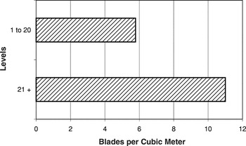
Pitahaya blade density by level.
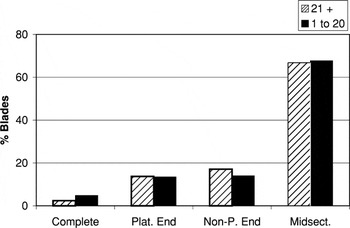
Blade morphology percentages by level.
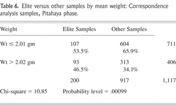
Elite versus other samples by mean weight: Correspondence analysis samples, Pitahaya phase.
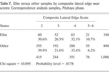
Elite versus other samples by composite lateral edge wear scores: Correspondence analysis samples, Pitahaya phase.
 You have
Access