

Introduction
Many host-parasite systems are characterized by an obligatory environmental stage in the parasite life-cycle. This stage can lead to transmission of the parasite between cohorts of individuals living in a particular environment, for instance sheep grazing on a pasture during the summer season or commercial broiler chickens raised from hatching to slaughter in 6 weeks. Complexity even increases if the host's immunity to the infection is only gradually built up, depending on ingested dose and re-infections. Such parasite-host systems can give complicated, unpredictable dynamics even with a relatively simple within-host infection model (Roberts et al. Reference Roberts, Smith, Grenfell, Grenfell and Dobson1995; Anderson, Reference Anderson1998; Roberts and Heesterbeek, Reference Roberts and Heesterbeek1998).
To obtain a better understanding of the dynamics of such complicated systems, we study a particular parasite-host system by using empirical experiments and theoretical models, namely Eimeria infections in chickens. Eimeria is a protozoan parasite of the gut and causes coccidiosis in chickens, resulting in production loss and sometimes severe intestinal damage (Allen and Fetterer, Reference Allen and Fetterer2002). There are 7 chicken-specific species, infecting particular sites in the gut and not inducing cross-immunity. Acquired immunity – mainly consisting of cytotoxic T lymphocytes against the intracellular schizont stage – can reduce the adverse effects of infection, but protection only gradually increases upon reinfection (Lillehoj and Lillehoj, Reference Lillehoj and Lillehoj2000; Yun et al. Reference Yun, Lillehoj and Lillehoj2000).
The dynamics of coccidiosis in chicken populations is due to interactions between different scales. First, there is interaction between intracellular parasite stages and the individual immune system. Second, there is dynamics within flocks, where excreted oocysts are again ingested resulting in subsequent infection generations until complete immunity has been built up. Third, there is transmission dynamics between subsequent flocks of chickens, where the number of infectious oocysts in the shed at the end of one production cycle sets the initial condition for the next cycle. Moreover, stochastic processes might be important in this system, especially in oocyst uptake from the environment, inducing heterogeneity in the population.
In a previous paper (Klinkenberg and Heesterbeek, Reference Klinkenberg and Heesterbeek2005) we were able to accurately describe the within-host dynamics with a discrete time model of the parasite life-cycle and a non-linear interaction with a single immune variable. Typical experimental results such as the relation between parasite uptake and excretion, and the gradually increasing immunity during trickle infections could be explained, and some model parameters were estimated. In this paper we take a next step and close the parasite life-cycle by including the relation between parasite excretion and subsequent uptake. By defining contamination level as the number of available oocysts per chicken in the shed, we will study the relation between initial contamination level of the environment, production damage and disease caused by the intracellular stages of the parasite, and the contamination level at the end of the broiler production cycle. Furthermore, we will study long-term intercohort dynamics, which are governed by the relation between initial and final contamination level. Finally, stochastic aspects, although important, will not yet be treated in this paper.
The model
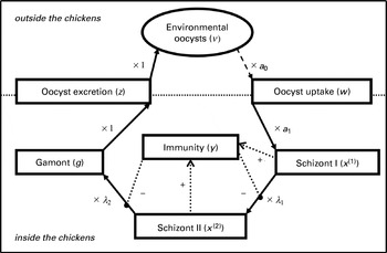
We have used the within-host model for Eimeria infections described by Klinkenberg and Heesterbeek (Reference Klinkenberg and Heesterbeek2005) as a basis for the full cycle model. The model is a linear description of the parasite life-cycle, starting with oocysts (w), and followed by 2 intracellular schizont stages (x (1) and x (2)) for asexual reproduction and 1 intracellular gamont stage (g) for sexual reproduction, each gamont becoming 1 oocyst to be excreted (z) (Fig. 1). All variables are dimensionless quantities, and the parameters a 1, λ1, and λ2 are the multiplication factors between the stages. Furthermore, the schizont stages interact with an immune variable y, governed by the parameters α (immunity survival, per time step), β (naïve growth, per schizont, per time step), and γ (booster-like growth, per schizont, per immunity unit, per time step). The model is formulated in discrete time, because of the distinct, successive developmental stages, and the time unit is ∼2 days, because that is the approximate time between the intracellular stages and it results in the correct interval between oocyst uptake and peak excretion for most Eimeria species (Allen and Fetterer, Reference Allen and Fetterer2002; Williams, Reference Williams2001):


In Klinkenberg and Heesterbeek (Reference Klinkenberg and Heesterbeek2005), we estimated the fecundity a 1λ1λ2 and the parameters β and m for 7 Eimeria species, and we combined experimental data and model observations to obtain reasonable values for the other parameters. A typical parameter set is used for the simulations and examples in this paper (Table 1). The initial value is 0 for all variables at the start of a chicken cohort, with the exception of w 0 (see below).
Schematic of the Eimeria cycle, the interaction with immunity, and re-uptake from the environment (model equation (1)). The solid lines and multiplication factors denote the progression through the infection cycle from uptake to excretion, the dotted lines indicate the interaction with the immune system through stimulation (arrows) and inhibition (large dots), and the dashed line refers to uptake of a fraction of oocysts from the environment.

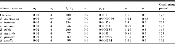
Parameter sets for the general model and the seven Eimeria species
(The values of a 0 and σ are derived in this paper, the other parameters are from estimations by Klinkenberg and Heesterbeek (Reference Klinkenberg and Heesterbeek2005). The far right column lists the oscillation periods in units of model time steps for the re-uptake model (1) in a single cohort.)

In this paper, we close the infection cycle, making w dependent on a new variable v, the contamination level, i.e. the per chicken number of sporulated oocysts in the environment (Fig. 1). Because sporulation, which is required for an oocyst to become infectious, takes about 1–2 days (Parry et al. Reference Parry, Barratt, Jones, McKee and Murray1992; Graat et al. Reference Graat, Henken, Ploeger, Noordhuizen and Vertommen1994; Waldenstedt et al. Reference Waldenstedt, Elwinger, Lundén, Thebo and Uggla2001; Allen and Fetterer, Reference Allen and Fetterer2002; McDougald, Reference McDougald and Saif2003), the transition from z to v takes one time step in the model. We consider the average infection dynamics in a population of chickens by assuming that this is equivalent to all chickens undergoing identical infection dynamics:


Here, a 0 is the uptake probability per oocyst, per time unit, and a proportion σ of the oocysts that are not ingested, survive to the next time step. At the start of a chicken cohort, v 0>0, and thus w 0>0.
Parameter values
The two new parameters require realistic values for our analyses and simulations. The parameter a 0 is the proportion of oocysts ingested from the environment per chicken per unit of time (2 days). Parry et al. (Reference Parry, Barratt, Jones, McKee and Murray1992) estimated the uptake rate to be 0·00008/h for a chicken of 2 weeks of age, though in his own model he used values ranging from 0·01 to 0·000001 because of the large uncertainty of the estimate. For our model, the estimate of 0·00008/h would result in a value a 0=0·0038/time unit, but experiments of our own (see Appendix) indicate a value of about 0·0102/time unit; we used a 0=0·01/time unit for our figures.
The parameter σ is the oocyst survival rate per unit of time, which was estimated by several authors. Long and Rowell (Reference Long and Rowell1975) sampled an entire shed at 62 sites, counted oocysts with an interval of 2 weeks, and measured a survival of 0·184, which is equivalent to σ=0·79 per time unit of 2 days. Reyna et al. (Reference Reyna, McDougald and Mathis1982) measured the decrease of viable oocysts by sampling every 3 days from litter, and inoculating naïve chickens with the samples; they measured a survival of 0·121 per 3 days, equivalent to σ=0·24 per 2 days. Parry et al. (Reference Parry, Barratt, Jones, McKee and Murray1992) reported a measured decay rate of 0·004/h, leading to σ=0·83, and Williams et al. (Reference Williams, Johnson and Andrews2000) estimated a weekly survival of 0·33, resulting in σ=0·71. These remarkably consistent estimates made us choose σ=0·5 per time unit for our figures.
Disease and production loss
Coccidiosis is an infection causing disease and production loss (McDougald, Reference McDougald and Saif2003). The adverse effects are due to damage of the intestinal epithelium: it hampers absorption of nutrients and severe infections induce bleedings and blood loss. Although the Eimeria species differ with respect to the damage caused by the different intracellular stages (McDougald, Reference McDougald and Saif2003), all intracellular stages (in the model, 2 schizont generations and the gamont) of the parasite cycle do cause damage, which is why we will use the sum of the abundances of the intracellular stages as a measure for damage: d t=x t(1)+x t(2)+g t. To determine the total damage during a broiler cohort, the maximum or cumulative damage could be used, but as in most cases the cumulative damage is dominated by a single maximum, they are almost equal. For simplicity, we will use the maximum number d max of intracellular stages at one time as a measure of damage during 1 cohort.
Results
Dynamics in a single cohort
We start by studying the dynamics within a chicken cohort. A convenient first step is to regard equilibrium states, and it turns out that, apart from the trivial disease-free equilibrium, there exists an endemic equilibrium, with

The levels of the other variables can be calculated accordingly, implying that with the default parameter set,  =15·7 and =516, and the steady-state oocyst excretion =261. Stability analysis (Edelstein-Keshet, Reference Edelstein-Keshet1988; we used Mathematica® for all calculations, simulation and plots) reveals that this equilibrium is unstable for all parameter sets used, and the long-term dynamics appear to consist of oscillations with periods between 41 and 253 time-units (Table 1). These oscillations are due to fractional amounts of environmental oocysts causing recurrent outbreaks in chickens that have almost completely lost their immunity (a well-known problem of deterministic models, Mollison (Reference Mollison1991)), but fortunately these unrealistic phenomena do not occur until long after the time-window of a chicken cohort in which we are interested: 17–30 time steps of 1·4 to 2·5 days. Therefore, the model is appropriate for our purpose.
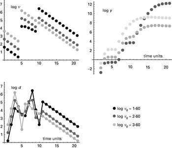
A detailed picture of the dynamics during such a cohort of 21 time steps is shown in Fig. 2. The model variables are plotted on a log-scale (base 10), as in all figures, and to avoid confusion we will only use log-transferred variables in the rest of the article. The cycle starts with naïve chickens in a contaminated environment, with initial per chicken contamination levels log v 0 of 1·60, 2·60, or 3·60. At first the oocyst levels decline, but at t=5 there is a large increase due to excretion and sporulation after the first passage through the chicken population, upon oocyst ingestion at t=0. This first passage is also observable as a damage peak at t=3 due to the gamont stage, and as an increase in immunity level y. The oocyst uptake at the subsequent times (t=1−4) is smaller, and therefore has a relatively small effect on oocyst level, damage, and immunity.
Dynamics within a single chicken cohort of 21 two-day time steps for the default parameter set. The plots show the environmental oocyst level log v, the immune level log y, and the damage level log d for 3 initial oocyst levels: log v 0=1·60, 2·60, and 3·60.

The large excretion at t=5 causes a sudden rise in oocyst uptake, resulting in a second infection generation with many more parasites than in the first generation, with a new damage peak at t=8 and an increase in immunity. The oocyst level in the log v 0=3·60 simulation does not visibly rise upon the second infection peak, but a second excretion peak does occur in the simulations starting with 1·60 and 2·60 log-oocysts. These simulations even show a third infection generation, with damage peak and immunity increase. Ultimately, the least damage (lowest d max) is observed in the log v 0=2·60 simulation, and the initial order of the environmental oocyst levels is reversed at the end.
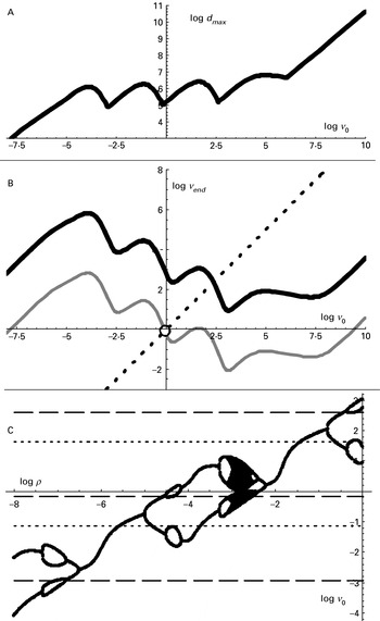
An important conclusion from Fig. 2 is that the dynamics within a cohort are determined only by the first ingested dose of each infection generation. This is clearly visible in Fig. 3A, where we plotted the function D, the damage level log d max as a function of the initial oocyst level log v 0. If log v 0 is larger than ∼2·5, the first infection generation determines the damage, either due to the gamont stage (log v 0<6) or due to the 2nd generation schizonts (the linear part). If log v 0 is between ∼−0·2 and ∼2·5, it is the 2nd generation that determines log d max, and with lower log v 0, the 3rd and 4th. Intermediate log v 0 values, when there is no single dominating infection generation (e.g. log v 0≈−0·2, or 2·5), result in local damage minima in Fig. 3A, a phenomenon that has also been observed experimentally (Graat et al. Reference Graat, Ploeger, Henken, De Vries Reilingh, Noordhuizen and Van Beek1996). It also suggests that it should be possible to create optimal contamination levels to minimize the adverse effects of coccidiosis infection, that is, if complete cleaning is not feasible.
Model results for the default parameter set. (A) Relation D between initial oocyst level log v 0 and maximum damage log d max during a single chicken cohort. (B) Relation V between initial oocyst level log v 0 and final oocyst level log v end (black line). The grey line indicates the initial oocyst level of the next cohort after cleaning with efficiency log ρ=−3; the intersection with the dotted line is the equilibrium log v 0 for subsequent cohorts. (C) Bifurcation diagram for the between-cohort dynamics of log v 0 as a function of the cleaning efficiency log ρ. The horizontal dashed and dotted lines indicate the log v 0 values corresponding to log d max minima and maxima, respectively.

An optimal contamination level should be achieved by optimally efficient cleaning, not necessarily maximally efficient. If it were possible to clean up to a desired contamination level irrespective of the oocyst level at the end of the previous cycle (e.g. log v 0=2·5 if Fig. 3A would apply), this would be ideal as long as the desired level can be reached with enough precision. Of course, the oocyst level at the end of the previous cycle should not be lower than the intended level.
It is more likely, however, that cleaning results in a proportion ρ of oocysts at the end of each production cycle (cohort) to set the initial level for the next cohort. Then, ρ should be chosen such that log v 0 is located at a local minimum of log d max (Fig. 3A), and that it results in the same log v 0=log ρ+log v end for the next cohort (in ordinary scale: v 0=ρv end), so that an optimal equilibrium is found. To see if this is possible, it will be necessary to study the dynamics between successive cohorts.
Dynamics between cohorts of chickens
The between-cohort dynamics is studied by regarding log v 0 in subsequent cohorts of chickens. Each log v 0 in cohort i is equal to the final oocyst level log v end in cohort i−1, corrected by cleaning efficiency log ρ: log v 0,i+1=log ρ+log v end,i. Thus, the between-cohort dynamics is determined by the function V, describing the relation between log v 0 and log v end (Fig. 3B), which happens to display a wave-like pattern also indicating an important role for the dominating infection generation (as we saw with damage). The between-cohort dynamics will be in equilibrium if log v 0,i+1=V(log v 0,i)+log ρ. The equilibrium log v 0 can be determined graphically, by determining the intersection point of V(log v 0,i)+log ρ with the diagonal line log v end=log v 0, e.g. if log ρ=−3, the equilibrium value is log v 0*=−0·06 with the default parameters (Fig. 3B).
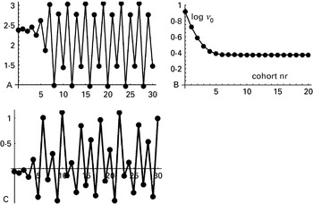
For optimal cleaning it will be necessary to choose ρ such that a minimum damage level is reached in each subsequent cohort. This requires stability of the subsequent log v 0 levels. Fig. 4 shows the between-cohort dynamics for log ρ=−3, −2, and 0, from which it appears that the equilibrium log v 0* may be stable, but that other between-cohort dynamics are also possible, like a 4-cycle or even chaos. Whether an equilibrium will be stable can be read from Fig. 3B: if the slope of the function V is between −1 and 1, the equilibrium is stable, otherwise it is not (Edelstein-Keshet, Reference Edelstein-Keshet1988). Thus, unstable equilibria can be expected if log ρ is chosen such that log v 0*≈−3, 0, or 3.
Dynamics of the initial oocyst level between successive chicken cohorts for the default parameter set, starting close to (A, C) or far from (B) the equilibrium. The plots show the dynamics for three values of the cleaning efficiency: log ρ=0 (A), −2 (B), and −3 (C). Cohort number on the X-axes; log v 0 on the Y-axes.

Although Fig. 3B can be used to predict stability, the type of unstable dynamics cannot be predicted. A bifurcation diagram (Fig. 3C) can be drawn to give this information. In Fig. 3C, the type of dynamics can be seen for each value of the cleaning efficiency log ρ, e.g. without cleaning there will be a 4-cycle, if log ρ=−2, the equilibrium will be stable, and if log ρ=−3, chaotic dynamics will appear. The values of log v 0 in the subsequent cycles can be read from the Y-axis of the bifurcation diagram, which makes it possible to look for values of log ρ resulting in minimum damage levels in each cycle. All minimum and maximum damage levels from Fig. 3 are indicated with (dashed and dotted) horizontal lines. It turns out that more efficient cleaning can indeed reduce log d max, e.g. when log ρ is decreased from −1·7 to −2·2, but that the damage minima cannot be reached in a stable equilibrium. Further reduction of log ρ might seem to be effective at first hand, but cyclic or choatic behaviour will result in less favourable cohorts as well.
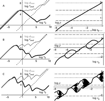
Unpredictable damage in subsequent cycles is caused by the combination of unstable dynamics on the one hand and large differences between peaks and troughs in the log v 0–log d max relation on the other hand. To understand how the different factors of the Eimeria dynamics affect these characteristics, we simplified the model to a description in infection generations only, so as to obtain separate functions for the different peaks in the V and D functions (see Supplementary material). Here we give the resulting insights by discussing the dynamics of some of the Eimeria species (Fig. 5).
The left panels depict the relations between initial oocyst level log v 0 and final oocyst level log v end (V, black lines) and between log v 0 and maximum damage log d max (D, grey lines) for 3 Eimeria species: (A) E. acervulina, (B) E. maxima, (C) E. tenella. The right panels show the bifurcation diagrams for the between-cohort dynamics of log v 0 as a function of cleaning efficiency log ρ for the same species; the dashed horizonal lines indicate the damage minima corresponding to the log d max graphs at the left.

The major difference between the default parameters and the parameters for E. acervulina are the multiplication factors between the different within-host stages: the fecundity of E. acervulina is much smaller. This has its effect in the horizontal distance (in the log v 0 direction) between the log d max and log v end peaks in Fig. 5A. The damage peaks become less pronounced, and the log v end peaks even disappear completely. The reverse can be observed for E. brunetti, where the differences between damage minima and maxima are large (not shown). Thus, high fecundity enhances variability in damage in relation to log v 0.
Another difference between E. acervulina and the default parameter set is the generation time. Because E. acervulina is known for its short pre-patent period (time between oocyst uptake and peak excretion) of only 5–6 days, a complete cycle length takes 7 days, including 1 day of sporulation (Graat et al. Reference Graat, Henken, Ploeger, Noordhuizen and Vertommen1994; McDougald, Reference McDougald and Saif2003), which means that time should be measured in units of 1·4 instead of 2 days. This causes a complete cohort to take 30 time steps and it changes the parameter σ, the oocyst survival in the environment, which becomes σ=0·51·4/2=0·62 to reach the same survival rate per day. It is the change in σ that affects the relation between log v 0 and log v end, as it is σ that determines the height differences between the peaks, in the E. acervulina case reflected in the slope of the decreasing part of the graph (the peaks being merged due to decreased fecundity as described above). Thus, the short generation time of E. acervulina prevents cyclic behaviour and provides the possibility of reaching a stable damage minimum in subsequent cycles by cleaning with an optimal efficiency, e.g. log ρ=−1·8 or −4·0 (Fig. 5A).
The value of m, the non-linearity in the immune effectiveness, determines the negative slope at the right of the individual peaks. Right of the right-most peak the slope tends to 1−m (the right-most peak has the slope of the single-infection model, studied by Klinkenberg and Heesterbeek, Reference Klinkenberg and Heesterbeek2005), and right of the other peaks the slopes go to 1−3m; however, these slopes are not always reached because of the next peak taking off. The effect of m is clearly seen in Fig. 5B and C for E. maxima (m=0·97) and E. tenella (m=1·51): E. tenella has a more pronounced damage differences and displays more types of between-cohort dynamics with 2-cycles, 4-cycles and chaos, whereas E. maxima dynamics is only stable or in a 2-cycle, with smaller differences between damage minima and maxima. Thus, non-linearity in the immune function promotes unstable dynamics, especially in combination with large fecundity causing large horizontal distances between the peaks of V.
Differences in the parameters β and γ, determining the growth of immunity, do not affect the shape of the functions D and V, only the position in the diagonal direction from the lower left to the upper right. Therefore, E. tenella (with low β and γ) has high log d max values and high final oocyst levels, whereas E. maxima has considerably lower levels. This does, however, not mean that production loss and health problems are more severe with E. tenella, since that is also (mainly) related to specific species characteristics in relation to the host.
Discussion
A major conclusion from the Eimeria re-infection model is that damage due to infections can be minimized by starting the infection process at intermediate oocyst contamination levels. This result was also observed experimentally (Graat et al. Reference Graat, Ploeger, Henken, De Vries Reilingh, Noordhuizen and Van Beek1996) and in a previous simulation study of coccidiosis dynamics (Henken et al. Reference Henken, Graat, Ploeger and Carpenter1994), but in those studies possible underlying mechanisms were not addressed. Here we did address this and determined that within-cohort dynamics are governed by the first dose of each infection generation, and damage is minimal if there is no single dominating infection generation. Moreover, we could show that it will often be impossible to achieve minimum damage at subsequent production cycles by removing a fraction of oocysts from the floor after each cycle, because that may lead to cyclic or chaotic between-cohort dynamics. Finally, we were able to see that unstable dynamics with large differences between minima and maxima are more likely in the following cases: if the parasite fecundity is high, if the oocyst decay rate is high, if the infection cycle is slow, and if there is a strong non-linearity in the immune dynamics.
Coccidiosis control in practice is best served by aiming at an initial oocyst level corresponding to minimal damage, which might be attained by optimal cleaning. Of course, cleaning as defined in our model is rather abstract when compared with the real world, where farmers probably just try to remove as many oocysts as possible, but the model can give an idea on the likelihood of improving the coccidiosis situation on a farm by changing the cleaning effort. Namely, if cleaning results in removal of a proportion of oocysts, there is no cleaning effort that results in minimum damage in subsequent cohorts. Thus, one should aim for a fixed oocyst level irrespective of the oocyst level at the end of the previous cohort, which could for instance be done by first cleaning to a very low oocyst level and then artificially infecting the environment up to a relatively high optimal level. An extra advantage of this strategy is that growth reduction in the beginning of the cycle is considered less harmful, as it can more easily be compensated for in later weeks.
Our understanding of Eimeria dynamics in subsequent chicken cohorts has been much improved by the model in this paper, but 3 aspects need further investigation: a more gradual and realistic excretion pattern resulting from each oocyst dose, differences in dynamics between individual chickens, and the spatial distribution of oocysts and chickens in a shed. Whereas our present model regards only peak excretions (4 time units after uptake) and averages in environmental contamination level, infection load and immunity, in reality excretion patterns are more gradual, oocysts are not evenly distributed within a shed, and individual chickens experience different (stochastic) uptake histories. It may be that differences between chickens and spatial heterogeneity will enhance the wave-like within-cohort dynamics, because each infection generation will reach a larger number of yet naïve chickens. However, more gradual excretion patterns are likely to smoothen within-cohort dynamics, as may heterogeneities, because infection generations of individual chickens will overlap. Then it remains to be seen to what extent damage minima and cyclic between-cohort dynamics are retained. The effects of individual heterogeneity and spatial processes are currently under investigation.
On a more abstract level – as elaborated on in the Supplemental Files – this paper dealt with a model of 2 variables, oocyst contamination v and immunity y, one of which was subject to resetting at regular time-intervals: each new cohort consisted of chickens with y 0=0. The other variable remained at its value, possibly multiplied by some constant factor ρ. This aspect of the model is similar to models of nematodes infecting sheep on a summer pasture (Roberts et al. Reference Roberts, Smith, Grenfell, Grenfell and Dobson1995; Roberts and Heesterbeek, Reference Roberts and Heesterbeek1998), nematodes infecting insects that only reproduce in the summer season (Dugaw et al. Reference Dugaw, Hastings, Preisser and Strong2004), childhood diseases spreading during the school year (Andreasen and Frommelt, Reference Andreasen and Frommelt2005), and insect-parasitoid dynamics on regularly harvested crops (Ives et al. Reference Ives, Gross and Jansen2000). A general insight from all these models is that regular resetting of variables often results in cyclic or chaotic dynamics, but specific cases will always require specific models because of the large differences in within-season/cohort dynamics.
We thank F. Velkers for providing experimental data to estimate the oocyst uptake rate. The research of J. A. P. H. is supported by the Netherlands Organisation for Scientific Research (NWO grant 918.56.620).
APPENDIX: Estimation of the parameter a 0
The experiments used to estimate a 0 will be published by Velkers et al. so here we only give a short summary of the experimental set-up, the type of data, and we explain the estimation method. Velkers et al. carried out 27 experiments with pairs of chickens, one of which was inoculated with oocysts of E. acervulina. They were housed in a floor cage, so that excreted oocysts could be ingested, enabling infection of the non-inoculated bird (contact bird) and continuous re-infection of both birds. This process was followed by counting oocysts from faeces samples on a daily basis. In 17 pairs (group A) the inoculation dose was 50 oocysts, and in 10 pairs (group B) 500 oocysts, but only 9 pairs of each group contained sufficient data for reliable estimations.
To estimate a 0 we needed for each pair the inoculation dose (w), the cumulative excretion of the inoculated chicken resulting from the inoculation dose (z (1)), and the cumulative excretion of the contact bird resulting from uptake of the first generation of excreted oocysts (z (2)). We assume the following relations to hold (Klinkenberg and Heesterbeek, Reference Klinkenberg and Heesterbeek2005):


The values of β, a 1, and m are as in Table 1, and f is the fecundity of the E. acervulina strain used in the experiment. The first equation describes the relation between oocyst uptake w (50 or 500) and the resulting excretion z (1), and it was used to estimate f by solving the equation for each experiment separately, and taking the geometric mean of all solutions. This resulted in an estimate of f=16054.
The second equation describes the relation between the excretion by the inoculated chickens z (1) and the first generation of excreted oocysts from the contact chickens z (2). The parameter p is the proportion of z (1) that is ingested by the contact chickens, and this can be estimated by solving the equation for each experiment separately, and taking the geometric mean of all solutions. This resulted in an estimate of p=0·0102. Because in the model it is only the first dose of each infection generation that appears to be relevant, we conclude that a 0=0·01.
SUPPLEMENTARY MATERIAL
To: A model for the dynamics of a protozoan parasite within and between successive host populations, by D. Klinkenberg and J. A. P. Heesterbeek
The model (1) was simplified in 2 steps: first, the within-cohort dynamics was described by subsequent infection generations, and second, approximations were made for the separate generations. We start with a few simplifying assumptions:
– α=1: waning of immunity is irrelevant due to continuous re-infection
– γ=β: precise estimates for γ are not available and the order of magnitude is correct
– a new immune variable
 is defined by the approximation . Note that .
Then, by regarding only the first ingested dose of each infection generation k (in original time: w t=a 0v t only for t=0, 5, 10, etc, otherwise w t=0), the dynamics are fully described by v and only. This results in the following model:


The new parameters are φ=(σ(1−a 0))5, the oocyst survival probability per infection generation, i.e. per 5 original time steps; r=a 0a 1λ1λ2, the maximum oocyst multiplication rate; and p=βa 0a 1, the immunity growth rate per oocyst per unit . Each broiler cohort consists of four infection generations. Because it is the gamont stage that causes most of the damage, damage can be described by d k=v k−φv k−1, the amount of oocysts excreted in generation k.
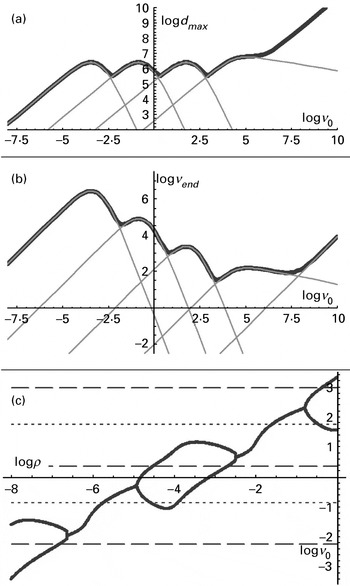
Figure A1 shows the functions V and D (defined in the main text) and the bifurcation diagram for model (A1). It appears that all typical features of the original model (1) as shown in Fig. 3 are present in the new model: the wavelike Fig. A1a and A1b, and the unstable dynamics with some cleaning rates in Fig. A1c; only the chaotic dynamics has disappeared. However, with other parameter sets (e.g. the E. brunetti parameter set) the simplified model is still capable of displaying chaotic dynamics.
Results of the simplified models (equations A1 in thick black lines and A2 in thin grey lines) for the default parameter set; (a) relation D between initial oocyst level log v 0 and maximum damage log d max during a single chicken cohort; (b) relation V between initial oocyst level log v 0 and final oocyst level log v end; (c) bifurcation diagram for the between-cohort dynamics of log v 0 as a function of the cleaning efficiency log ρ.

The next step was to define functions for the damage level and the final oocyst level due to each infection generation, Dk and Vk (like D and V, these are defined on the log scale). We observe that Dk=Vk−(4 – k) log φ, k⩾1, because damage is determined by the number of gamonts which is equal to the number of excreted oocysts. This leaves us to find expressions for all Vk, starting with k=0 and k=1:


For excretion in generations k=2, 3, and 4 to be relevant for the final oocyst level, immunity should still be small in generation k−1. As long as the oocyst level and immunity are small in the early generations (v≈0 and y≈1), model (2) can be approximated by v k+1=rv k and y k+1=1+pλ1v k. Therefore, the level of immunity can be described in terms of the oocyst level, y k=1+pλ1v k/r, which leads to the following function for v k+1:

Thus, Vk, k>1, is equal to:

All functions Dk and Vk are plotted in Fig. A1 (thin grey lines).
As indicated in the main text, unpredictable damage hinges on unstable dynamics and large differences between minima and maxima in D. The condensed model (A2) gives insight into the role of the different parameters:
– the distance between the peaks of Dk and Dk+1 (and between Vk and Vk+1), k>1, in the log v 0 direction is equal to log r. The distance between the peaks of D1 and D2 (and between V1 and V2) also increases with increasing log r. Therefore, an increase in log r results in larger differences between damage minima and maxima, and it results in a larger domain in V with negative slopes <−1.
– the distance between the peaks of Vk and Vk+1, k>1, in the log v end direction is equal to log φ. There is no effect on D, but the domain in V with possibly unstable between-cohort dynamics increases if log φ decreases.
– the slopes left of the peaks of all Vk is 1, the slope right of the peak of V1 is 1−m, and the slopes right of the peaks of all Vk, k>1, is 1−3m. Thus, the minimum slopes for realistic values of m are smaller than −1 and these are always close to the minima in D. A larger m will result in smaller minima in D and possibly less stable between-cohort dynamics.
– the minimum slopes 1−3m are due to two terms in Vk, k>1: −2mlog (…) and −mlog (…), which contribute to Vk only if pλ1r k−2v 0 and pr k−1v 0 are notably larger than 0. The peak between increase (slope=1) and decrease (slope=1−3m) will be sharpest if both terms are of the same order of magnitude, that is if λ1≈r, because that will cause the most prominent transition between maximum and minimum slope. Sharper peaks will result in a sharper profile in D, and in a larger domain in V with unstable dynamics.
– an increase in log p causes a translation of the series of peaks in the (−1, −1) direction. This does not affect the qualitative behaviour of the between-cohort dynamics.