1. Introduction
In combinatorics, the Stirling numbers of the second kind, denoted by  $\{ \}$, count the number of ways to partition a set of n elements into k non-empty subsets. Moreover, the r-Stirling numbers of the second kind (Broader (1984)) with parameters
 $r\leq k \leq n$ enumerate the partitions of a set of n elements into k non-empty, disjoint subsets such that the first r elements are in distinct subsets. Then, by using similar arguments as the one that relates the Stirling and Bell numbers, the r-Bell numbers or generalised Bell numbers (MezÖ (Reference MezÖ2011)),
 \begin{equation}B_{n,r}=\sum_{k=0}^n {{n+r}\brace {k+r}}_r, \end{equation}
represent the counts of the partitions of a set with  $n+r$ element such that the first r elements are in distinct subsets in each partition, where
 ${{}\brace {}}_r$ are the r-Stirling numbers of the second kind. As a result of (1), the r-Bell polynomials are defined as
 \begin{equation}B_{n,r}(x)=\sum_{k=0}^n {{n+r}\brace {k+r}}_r x^k.\end{equation}
On the other hand, the study of probabilistic families to describe count data has been of great interest in actuarial statistics providing alternatives to the Poisson and negative binomial distributions. Modelling the expected frequency based on insurance policy characteristics via count regression analysis is crucial for the insurance practice. For a comprehensive survey of probabilistic models for panel data based on generalisations of the Poisson and negative binomial distributions, the reader is referred to Boucher et al. (Reference Boucher, Denuit and GuillÉn2008) and references therein. In this paper, a three-parameter discrete distribution, the  $r{\mathcal B}ell$ distribution, is introduced based on a series expansion of the r-Bell polynomials. This family of distributions possesses interesting statistical and actuarial properties. In this sense, this family of distributions is a special case of the multiple Poisson process, and its probability mass function can be either unimodal or bimodal. Also, it nests the Poisson distribution and the recently proposed Bell distribution (Castellares et al. (Reference Castellares, Lemonte and Moreno-Arenas2019), Castellares et al. (Reference Castellares, Ferrari and Lemonte2018)) and Bell–Touchard distribution (Castellares et al. (Reference Castellares, Lemonte and Moreno-Arenas2019)) that have not been discussed in the actuarial literature. The probabilities of the model can be computed by a recursive formula that allows us to calculate the probability function of the amount of the aggregate claims in the collective risk model in terms of an integral equation. Furthermore, univariate and bivariate regression models of this family of distributions are presented by parameterising the mean of the distribution as a function of explanatory variables. The latter regression model, which is derived by using the Sarmanov distribution, explains the model dependency in bivariate settings with given marginals. This bivariate regression model is used to describe the number of out-of-use and parking claims jointly. This family constitutes an alternative to other traditionally used distributions to describe count data, such as the negative binomial and Poisson-inverse Gaussian models.
The rest of the paper is organised as follows. In Section 2, we illustrate the genesis of the  $r{\mathcal B}ell$ family of distributions via r-Bell polynomials, and some special cases of this family are presented. In Section 3, a recurrence relation to calculate its probabilities is provided. Moreover, it is shown that this probabilistic family is a special case of the multiple Poisson process. Finally, some of its relevant properties are analysed, and its relationship with the natural exponential family of probability distributions is examined. In Section 4, some actuarial results are discussed. Here, the implications of the
 $r{\mathcal B}ell$ distribution in the collective risk model are examined. Also, the Esscher premiums in the collective risk model is obtained. In Section 5, univariate and bivariate regression models associated with this family of distributions are analysed. Simulation analysis and applications are given in Section 6, where real datasets of automobile insurance are considered. Lastly, the conclusions and further extension of this work are given in Section 7. All the proofs are given in the Appendix.
2. Genesis of the New Family of Distributions
Let us consider the double generating function of the r-Stirling numbers given by Broder (Reference Broder1984)
 \begin{equation} \exp\left\{\alpha \left(e^\theta -1\right)+r\theta \right\} = \sum_{y=0}^{\infty} B_{y,r}(\alpha)\frac{\theta^y}{y!},\end{equation}
where the coefficients  $B_{y,r}(\alpha)$ are the r-Bell polynomials that satisfy
 \begin{equation} B_{y,r}(\alpha)=\frac{1}{e^\alpha} \sum_{k=0}^{\infty} \frac{(k+r)^y}{k!}\alpha^k.\end{equation}
The r-Bell polynomials can also be expressed by the Bell polynomials (Bell (Reference Bell1934a) and Bell (Reference Bell1934b)) via the following formula:
 \begin{equation}B_{y,r}(\alpha)=\sum_{k=0}^{y} r^k\binom{y}{k}B_{y-k}(\alpha),\end{equation}
where  $B_{y-k}(\alpha)$ are the Bell–Touchard polynomials (Touchard (Reference Touchard1933)).
Remark 1 The r-Bell polynomials can be expressed as
 \begin{equation} B_{y,r}(\alpha)=\sum_{k=0}^{y} \left\lbrace \begin{array}{c}y+r\\ k+r\end{array} \right\rbrace_r \alpha^k = \sum_{k=0}^{y} \left( \sum_{i=0}^{y}\binom{y}{i}\left\lbrace \begin{array}{c}i\\ k\end{array} \right\rbrace r^{y-i} \right) \alpha^k,\end{equation}
where  $\left\lbrace \begin{array}{c}y+r\\k+r\end{array} \right\rbrace_r$ are the r-Stirling numbers of the second kind (see Broder (1984)).
The first few values of the r-Bell polynomials are given as follows:
 \begin{align*}B_{0,r}(\alpha) &= 1,\,\,B_{1,r}(\alpha) = \alpha + r,\,\, B_{2,r}(\alpha) = \alpha^2 + (2r + 1)\alpha + r^2,\,\,\dots\end{align*}
By taking in (3) and (4)  $r=0$ and
 $\alpha=1$, the Bell polynomials, that is
 $B_{y,0}(1)$, are obtained. Castellares et al. (Reference Castellares, Ferrari and Lemonte2018) derived the Bell distribution with probability mass function (PMF) given by
 $p_Y(y)= \exp \left\{1-e^\theta\right\} \frac{\theta^y}{y!}B_{y,0}(1), \, y=0,1,\dots$ Also, by choosing
 $r=0$, the Bell–Touchard polynomials are received. By using these polynomials, the Bell–Touchard distribution was introduced in Castellares et al. (Reference Castellares, Lemonte and Moreno-Arenas2019) with PMF
 $p_Y(y)= \exp \left\{\alpha \left(1-e^\theta \right)\right\} \frac{\theta^y}{y!}B_{y,0}(\alpha), \, y=0,1,\dots$. Obviously, when
 $r=1$ and
 $\alpha=0$,
 $B_{y,r}(\alpha)$ reduce to 1, and the Poisson distribution is obtained.
By considering (3) and (4), we define the three-parameter  $r{\mathcal B}ell$ family of distribution as follows.
Definition 1 A discrete random variable Y has a  $r{\mathcal B}ell$ distribution if its PMF is given by
 \begin{equation} p_Y(y)= \exp \left\{-\alpha \left(e^\theta -1\right)-r\theta\right\} \frac{\theta^y}{y!}B_{y,r}(\alpha), \quad y=0,1,\dots\end{equation}
where  $r>0, \theta>0, \alpha>0$ and
 $B_{y,r}(\alpha)$ are the r-Bell polynomials in (6). We denote a random variable Y that follows (7) as
 $Y\sim r{\mathcal B}ell(r,\alpha,\theta)$.
3. Distributional Properties
In this section, some distributional properties of the  $r{\mathcal B}ell$ distribution are presented. First, the PMF given in (7) can also be expressed in terms of the following recursive relation to compute their probabilities.
Proposition 1 The PMF of the  $ r{\mathcal B}ell$ distribution follows the recursive relation
 \begin{equation}p_Y(y)=\frac{r \theta}{y} p_Y(y-1) +\frac{\alpha \theta}{y} \sum_{k=0}^{y-1}\frac{\theta^{y-k-1}}{(y-k-1)!} p_Y(k), \quad y=1,2,\dots\end{equation}
with  $p_Y(0)=\exp\{-\alpha \left(e^\theta -1\right)-r\theta\}$.
It can be noted that for any value of r and  $\alpha$,
 $p_Y(0)\rightarrow 1$ as
 $\theta \rightarrow 0$, which implies that the
 $ r{\mathcal B}ell$ distribution is degenerated at 0 for small values of
 $\theta$. Moreover, the ratio
 $p_Y(1)/p_y(0)=\left(r+\alpha\right)\theta$ is less than one for
 $\theta <1/(r+\alpha)$ indicating that the modal value is located at zero. The sequence of the r-Bell polynomials
 $\lbrace B_{y,r}(\alpha), y\in \mathbb{N} \rbrace$ for
 $\alpha>0$ is log-convex (see Yan et al. (Reference Yan, Zhang and Xu2019)). The log-concavity of the
 $ r{\mathcal B}ell$ distribution is proved in the Lemma 7 given in the Appendix.
Proposition 2 The  $r{\mathcal B}ell(r,\alpha,\theta)$ distribution is strongly unimodal for either
 $(0<\alpha<1) \cap (\sqrt{\alpha}-\alpha<r<\alpha)$ or
 $\left(\alpha>1 \cap r>0\right).$
Proposition 3 The condition for the PMF of the  $r{\mathcal B}ell(r,\alpha,\theta)$ distribution to be bimodal is
 $(0<r<\sqrt{\alpha}-\alpha) \cap (0<\alpha<1) \cap \left(\frac{2(r+\alpha)}{(r+\alpha)^2+\alpha}<\theta<\frac{1}{r+\alpha}\right)$.
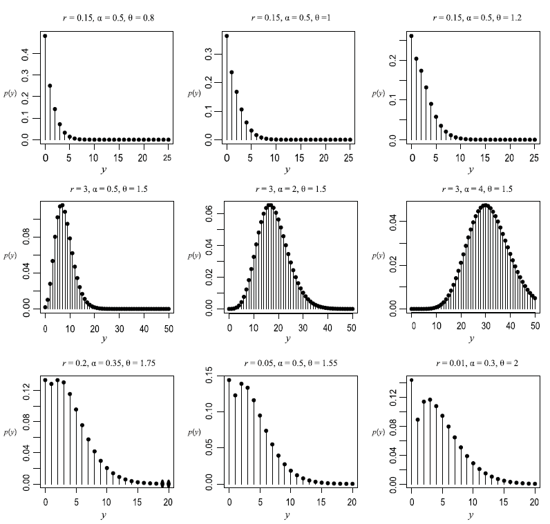
Figure 1 depicts different graphs of the PMF of the  $r{\mathcal B}ell$ distributions for various combinations of parameters r,
 $\alpha$ and
 $\theta$. It is noted that if the triplet
 $(r, \alpha, \theta)$ satisfies
 $\theta< \frac{1}{r+\alpha}$, the mode is at zero and the PMF has a unique modal value for different combinations of parameters satisfying Proposition 2. This is verified by the graphs in the top row of Figure 1. The PMF tends to be symmetric when the mean of (7) increases, as is observed in the second row. Further, the bimodality of the PMF can be noticed in the graphs of the last row of Figure 1.
Graphs of the PMF of the  $r{\mathcal B}ell(r,\alpha,\theta)$ distributions for various combinations of parameters r,
 $\alpha$ and
 $\theta$.

Lemma 1 below, due to JÁnossy et al. (Reference JÁnossy, RÉnyi and AczÉl1950), which is stated without proof, will be used to show that the  $r\mathcal{B}$ell distribution is a special case of a multiple Poisson process. Multiple Poisson processes allow the occurrence of multiple events (see JÁnossy et al. (Reference JÁnossy, RÉnyi and AczÉl1950)). A multiple Poisson process is a Markovian process with independent increments where the probability of occurrence of more than one event in a short period (0,t) is non-negligible relatively to the probability of the occurrence of a single event.
Lemma 1 Let us consider events occurring in time and let us impose that the process is homogeneous in time, that is we assume that the probability of exactly k events occurring in the interval  $(t_1, t_2)$ depends only on the length
 $t= t_2-t_1$ of this interval and let this probability be denoted by
 $W_k(t)$, for
 $k = 0, 1, 2,\dots$. Also, the process is of Markovian type, that is the number of events occurring during the time interval
 $(t_3, t_4)$ is independent of the numbers of events occurring during the time interval
 $(t_1, t_2)$ provided that
 $t_1 < t_2 \le t_3 < t_4.$ Then, We have that
 \begin{equation*}W_k(t)\ge 0 \qquad \text{and} \qquad \sum_{{k=0}}^{\infty}W_k(t)=1 \quad \qquad \text{for any} \quad t\ge 0,\end{equation*}
further
 \begin{equation*}W_0(0)=1 \qquad \text{and thus} \qquad W_k(0)=0 \quad \qquad \text{for} \quad k= 1,2,\dots\end{equation*}
It is also verified that
 \begin{equation} W_k(t)= \exp\left\lbrace-t \sum_{n=1}^{\infty} c_n\right\rbrace \sum_{s_1+2s_2+\dots+k s_k=k}\frac{(c_1 t)^{s_1}(c_2 t)^{s_2}\dots({{}c_k} t)^{s_k}}{s_1!s_2!\dots s_k!}\end{equation}
for a sequence of constants  $\{c_n;n\geq 1\}$ such that
 $c_n\geq 0$ and
 $\sum_{n=1}^\infty c_n$ is convergent.
The following theorem allows us to associate the  $r{\mathcal B}ell$ distribution with parameters
 $r,\alpha,\theta> 0$, to the distribution of a multiple Poisson process (with rates
 $c_n$).
Theorem 1 Let us consider a sequence  $\lbrace c_n\rbrace$, defined as
 $c_n=(\alpha+r)\theta,$ for
 $n=1$ and
 $c_n=\displaystyle \frac{\alpha \theta^n}{n!},$ for
 $n\ge2$, with
 $\theta>0$. For the time interval length
 $t=1$, we have
 \begin{equation*}W_k(1):=W_k=\exp \left\{-\alpha \left(e^\theta -1\right)-r\theta\right\} \frac{\theta^k}{k!}B_{k,r}(\alpha),\end{equation*}
where  $B_{k,r}(\alpha)$ are the r-Bell polynomials in (6).
Proposition 4 Let  $Y\sim r{\mathcal B}ell(r,\alpha,\theta)$, where
 $r,\alpha,\theta>0$. Then, the probability generating function (PGF) of Y is
 \begin{equation}G_Y(s)=\mathbb{E}(s^Y)=\exp\left\{\alpha\left(e^{s\theta}-e^{\theta}\right)+r\theta(s-1)\right\}, \quad |s|<1.\end{equation}
Proposition 5 If  $X\sim{\mathcal{BT}}(\alpha,\theta)$ and
 $Z\sim {\mathcal P}(r\theta)$ are independent, then the random variable
 $Y=X+Z\sim r{\mathcal B}ell(r,\alpha,\theta)$.
Remark 2 By using Proposition 9 in Castellares et al. (2019), the random variable  $X\sim \mathcal{BT}(1,\theta)$ can be expressed as
 $X= \sum_{i=1}^N T_i$, where
 $T_i$ for
 $i=1,2,\dots$ is a sequence of independent and identically distributed random variables that follow a zero-truncated Poisson distribution with parameter
 $\theta>0$ and N, independent of the sequence, has a Poisson distribution with parameter
 $(e^{\theta}-1)$. The zero-truncated distribution is the conditional probability distribution of a Poisson random variable, given that the value of the random variable is not zero (see Johnson et al. (2005) for more details).
Proposition 6 If  $Y_i$,
 $i=1,2,\dots,n$ are independent non-negative integer-valued random variables such that
 $Y_i\sim r{\mathcal B}ell(r_i,\alpha_i,\theta)$, then
 $\sum_{i=1}^{n}Y_i \sim r{\mathcal B}ell(\sum_{i=1}^{n}r_i,\sum_{i=1}^{n}\alpha_i,\theta)$.
Remark 3 A method to generate random variates from the  $r{\mathcal B}ell(r,\alpha,\theta)$ distribution is described as follows: (i) Generate u from U (0,1); (ii) find the positive integer i, with
 $i=0,1,\dots$, such that
 $F_Y( i-1) < u\leq F_Y( { i} )$ and (iii) return
 $y=i$, with
 $F_Y(i)=\sum_{j=0}^{i}p_Y(j)$, where
 $p_Y(j)$ is the PMF of the
 $r{\mathcal B}ell(r,\alpha,\theta)$ distribution evaluated at j.
Proposition 7 Let  $Y\sim r{\mathcal B}ell(r,\alpha,\theta)$ with
 $r>0,\alpha>0$ and
 $\theta>0$. Then, the cumulant generating function(CGF) is given by
 \begin{equation*}\mathbb{K}(t)=\alpha \left(e^{\theta e^t}-e^{\theta}\right)+r\theta(e^t-1),\,\,\text{with}\,\,t\in \mathbb{R}.\end{equation*}
The cumulants take form as  $\kappa_n=r\theta+\alpha e^{\theta}B_{n}(\theta),$
 $n\in \mathbb{N}$, where
 $B_n(\theta)$ are the Bell–Touchard polynomials (see Castellares et al. (2019)).
Note that the moment generating function (MGF) can be derived by exponentiating the CGF.
Remark 4 By using the above result, the first four central moments of the  $r{\mathcal B}ell$ distribution are
 \begin{eqnarray*}\mathbb{E}(Y)&=&\kappa_1= r\theta+\alpha \theta e^\theta,\\Var(Y)&=& \kappa_2= r\theta+\alpha \theta (1+\theta)e^\theta,\\\mu_{3}&=& \kappa_3= r\theta+\alpha \theta (1+3\theta+\theta^2)e^\theta, \\\mu_{4}&=& \kappa_4+2\kappa_2^2= r \theta + 3 \left(r\theta + \alpha \theta e^\theta (1+\theta)\right)^2 + \alpha \theta e^\theta \left(1+7 \theta + 6\theta^2 + \theta^3\right).\nonumber\end{eqnarray*}
The dispersion, defined as  $I_d=\displaystyle\frac{{Var}(Y)}{\mathbb{E}(Y)}$, is given by
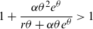 $1+\displaystyle\frac{\alpha \theta^2 e^\theta}{r\theta+\alpha \theta e^\theta} > 1$ for all
 $r,\alpha,\theta>0$ which implies that the
 $r{\mathcal B}ell$ distribution is overdispersed for
 $\alpha>0$ and hence suitable for modelling count data with overdispersion. Further, the skewness,
 $\varsigma_3=\displaystyle\frac{\kappa_3}{\kappa_1}-1$ (Puig and Valero (Reference Puig and Valero2006)) for the
 $r{\mathcal B}ell$ distribution is given by
 $(I_d-1)(3+\theta)>0$, suggesting that the skewness of the
 $r{\mathcal B}ell$ distribution is larger than that one of the Poisson distribution with the same mean. Finally, the
 $r{\mathcal B}ell$ distribution belongs to the natural exponential family with known r and
 $\alpha$ since
 \begin{equation*}p_Y(y)= \exp \left\{y\lambda-b(\lambda)- c(y)\right\}, \quad y=0,1,\dots\end{equation*}
with  $\lambda=\log \theta$,
 $b(\lambda)=\alpha \left(e^{e^{\lambda}}-1\right)+r\,e^{\lambda}$ and
 $c(y)=\log y!-\log B_{y,r}(\alpha)$. From these expressions, the mean and variance can be easily derived.
4. Some Actuarial Results
Some applications of the  $r{\mathcal B}ell$ distribution in risk theory are considered here. First, we derive the Esscher premium for this family of probability distributions. Although this premium principle is not suitable for practical purposes, for example, it does not preserve some desirable risk orderings; however, it is mathematically appealing, and it satisfies interesting properties (see Kamp (Reference Kamp1998)). The Esscher premium is the premium
 $\mathbb{P}$ that minimises the expected loss for the insurer when using the specific loss function
 $L(x,\mathbb{P})=(x-\mathbb{P})^2 e^{hx}$, with
 $h>0$.
Let  $Y\sim r{\mathcal B}ell(r,\alpha,\theta)$, where
 $r,\alpha,\theta>0$, the Esscher transform of Y is a random variable E with MGF given by
 $M_E(t)=M_Y(t+h)/M_Y(h)$, where
 $M_y(h)$ is the MGF of the
 $r{\mathcal B}ell$ distribution with parameter
 $h>0$.
Result 1 The Esscher premium of Y is given by
 \begin{equation}\mathbb{P}=\alpha\tilde \theta e^{\tilde\theta}+r \tilde \theta, \quad \text{where}\,\,\,\tilde\theta=\theta e^{h}\,\,\,\text{with}\,\,h>0.\end{equation}
Let Y be the number of claims in a portfolio of policies in a fixed time period. Let  $X_i$,
 $i=1,2,\dots$ be the ith claim size and the aggregate claims generated by the portfolio in the period under consideration
 $S=X_1+X_2+\ldots +X_Y$. We will assume that the claim sizes (
 $X_i$’s) are independent and identically distributed and independent of Y with common cumulative distribution function (CDF)
 $F(\cdot)$, common probability density function (PDF)
 $f(\cdot)$ and common MGF given by
 $M_X(\cdot)<\infty$.
Result 2 The Esscher premium of S, that is  $\check S$ is given by
 \begin{equation}\mathbb{\check P}=(\alpha\check \theta e^{\check\theta}+r \check \theta) \,\mathbb{E}(\check X), \end{equation}
where  $\check\theta=\theta M_X(h)$ with
 $h>0$ and
 $\check X$ is the Esscher transform of X.
Now, we discuss the implications of this distribution in the collective risk model. The CDF of the aggregate claims size S is (see Klugman et al. (2008))
 \begin{equation}F_S(x)=\sum_{k=0}^{\infty}p_Y(k) F^{k \ast}(x)\end{equation}
where  $F^{k \ast}(x)$ denotes the k-fold convolution of the CDF
 $F(\cdot)$ and
 $p_Y(k)$ as in (7). In order to derive (13), we need a recursive formula to compute the PMF of the
 $r{\mathcal B}ell$ distribution which is given in the following lemma. Then, this result is used to calculate the PDF/PMF of the aggregate claims amount.
Lemma 2 By denoting the PMF of the  $r{\mathcal B}ell$ distribution by
 $p(y;r,\alpha,\theta)$, then this PMF can be evaluated by the recursive formula
 \begin{equation} p_Y(y;r,\alpha,\theta)=\frac{\alpha \theta e^{-\theta}}{y} p_Y(y-1;r+1,\alpha,\theta) + \frac{r\theta}{y} p_Y(y-1;r,\alpha,\theta), \quad y=1,2,\dots\end{equation}
Theorem 2 If the claims sizes are absolutely continuous random variables with PDF f(x) and CDF F(x) for  $x\geq 0$ with
 $ F(0)=0$, then the PDF/PMF
 $g_S(x;r,\alpha,\theta)$ of the compound
 $r{\mathcal B}ell$ distribution satisfies the integral equation:
 \begin{align}f_S(x;r,\alpha, \theta) =\, & e^{-\alpha \left(e^\theta-1 \right)-r\theta} + \alpha \theta e^{\theta} \int_{0}^{x} \frac{y}{x}f_S(x-y;r+1,\alpha,\theta)f(y)dy \nonumber \\ & + r\theta \int_{0}^{x} \frac{y}{x}f_S(x-y;r,\alpha,\theta)f(y) dy,\end{align}
with  $\Pr\{S=0\}= p_Y(0;r,\alpha,\theta)$.
can be solved numerically utilising the theory of Volterra integral equations. However, if the claims size distribution is discrete, then by interchanging integral  $\int_{0}^{x}$ by
 $\sum_{y=0}^{x}$, (see Rolski et al. (Reference Rolski, Schmidli, Schmidth and Teugels1999) p. 119), the recursion formula of compound
 $r{\mathcal B}ell$ distribution is
 \begin{align*}f_S(x;r,\alpha, \theta) =\, & e^{-\alpha \left(e^\theta-1 \right)-r\theta} + \alpha \theta e^{\theta} \sum_{y=0}^{x} \frac{y}{x}f_S(x-y;r+1,\alpha,\theta)f(y) \\& + r\theta \sum_{y=0}^{x} \frac{y}{x}f_S(x-y;r,\alpha,\theta)f(y).\end{align*}
If the individual claim amounts are integer valued with common PMF denoted by  $f_k$, with
 $k=1,2,\dots$ and PGF
 $\tilde f(s)=\sum_{k=1}^{\infty}f_k s^k$ with
 $|s|<1$, then the PGF of S is given by
 \begin{equation*}G_S(s)=\exp\left\{\alpha\left(e^{\tilde f(s)\theta}-e^{\theta}\right)-r\theta(1-\tilde f(s))\right\}, \quad |s|<1.\end{equation*}
5.
 $r{\mathcal B}ell$ Regression Models

In this section, univariate and bivariate regression models associated with the  $r{\mathcal B}ell$ distribution are presented.
5.1 The univariate $\textbf{{r}}{\mathcal B}\textbf{{ell}}$ regression model

Let us now consider a response variable  $Y_{i}$ denoting the counts and a vector of covariates
 ${x_i}=(x_{i1},\dots,x_{ip})^{\top}$, including an intercept, related to the ith observation that designates a weight of observable characteristics with
 $i=1,2,\dots,n$. By writing
 $\mu=\alpha\theta e^{\theta}+r\theta$, we will assume that that
 $Y_{i}|\mu_{i} \sim r{\mathcal B}ell(\theta,r,\mu_i)$ with
 $\mu_{i}=\mathbb{E}(Y_{i}|{\bf{x_i}}^{\top})=\exp\{\log(\xi_i)+{\bf{x_i}}^{\top}{\underline\beta}\}$, where
 ${\underline\beta}=(\beta_{1},\beta_{2},\dots,\beta_{p})^{\top}$ is a vector of regressors and
 $\xi_i$ is the time exposure of the ith observation. Let us now suppose that
 $(y_{i},{\bf{x_{i}}}^{\top})$,
 $i=1,\dots,n$ are n independent realisations of this model where
 $y_{i}$ is the response variable,
 $\bf{x_{i}}^{\top}$ a vector of explanatory variables and
 $\eta_i=\bf{x_{i}}^{\top} \underline{\beta}$ is the linear predictor. Then,
 ${Var}(Y_i|{\bf{x_i}}^{\top})=\mu_i+\theta (\mu_i-r\theta)$. The log link guarantees a non-negative value for the conditional mean. Additionally, as it is verified that
 ${Var}(Y_{i}|{\bf{x_i}}^{\top})> \mathbb{E}(Y_{i}|{\bf{x_i}}^{\top})$, this model is overdispersed. Then, the log-likelihood is given by
 \begin{align} \ell(\underline \beta,r,\theta) =\, &\left(e^{-\theta } -1\right)\sum_{i=1}^{n}\left(\frac{\mu_i}{\theta}-r\right)+\log\theta\sum_{i=1}^{n}y_i -\sum_{i=1}^{n} \log y_i !\nonumber\\[4pt]& + \sum_{i=1}^{n} \log B_{y_i,r}\left(\frac{\mu_i}{\theta}-\frac{r}{\theta}\right).\end{align}
Maximum likelihood estimation (MLE) for this regression model involves setting the partial derivatives of the log-likelihood function with respect to regression coefficients  $\beta_{j}$ with
 $j=1,\dots,p$, r and
 $\theta$ equal to zero, these equations are not reproduced here. In practice, we have directly maximised the function (16) by using different maximum search methods available in the FindMaximum built-in function in the Mathematica software package. These methods include the Newton–Raphson, Principal Axis and the Broyden–Fletcher–Goldfarb–Shanno (BGGS) algorithms. Similar results were obtained for these optimisation methods by using different starting values. However, we have not been able to show that the optimal solution corresponds to a global maximum of (16) by the difficulty to prove that the log-likelihood function is concave. The standard errors of the estimates can be approximated by inverting the Hessian matrix. Note that we use the observed information matrix rather than Fisher’s information matrix since the latter cannot be derived since it involves calculating moments of expressions that include the r-Bell polynomials.
5.2 The bivariate $\textbf{r}{\mathcal B}\textbf{ell}$ regression model

In the following, we consider a bivariate  $r{\mathcal B} ell$ regression model (
 $Br{\mathcal B} ell$) by using the Sarmanov distribution. This family provides a favourable model for bivariate regression models (see BolancÉ and Vernic (Reference BolancÉ and Vernic2019)), and it is used to explain the model dependency in bivariate settings with given marginals. Sarmanov’s distribution can be defined in the discrete, as well as in the continuous case. We say that the random vector
 $(Y_1,Y_2)$ follows a bivariate Sarmanov’s distribution if its joint density is given by
 \begin{equation*}f(y_1,y_2)=f_1(y_1)f_2(y_2)(1+\omega\phi_1(y_1)\phi_2(y_2)),\end{equation*}
where  $f_j(\cdot)$,
 $j=1,2$ are the corresponding marginal densities,
 $\phi_j(\cdot)$ are bounded non-constant kernel functions and
 $\omega$ is a real number such that
 \begin{eqnarray*}\int_{-\infty}^{\infty}\phi_j(y_j)f_j(y_j)dy_j&=&0, \,{\,j=1,2,} \\1+\omega\phi_1(y_1) \phi_2(y_2)&\geq& 0,\;\forall\; (y_1,y_2)\in \mathbb{R}^2.\end{eqnarray*}
By taking  $\phi_j(y_j)=e^{-y_{j}}-\mathbb{E}\left(e^{-Y_{j}}\right)$, Papageorgiou and Piperigou (Reference Papageorgiou and Piperigou1997) derived the bivariate short and some related distributions, also Famoye (Reference Famoye2010) derived a bivariate negative binomial regression model. The same model was recently used in actuarial settings (Liu and Pitt (Reference Liu and Pitt2017)) to analyse claims frequency data in automobile insurance. Let n denote the sample size and
 $Y_{ij}$ with
 $i=1,\dots,n$ and
 $j=1,2$ denote the count regression model and a vector of covariates
 ${x_{ij}}=(x_{ij1},\dots,x_{ijp})^{\top}$, that is the same set of covariates as possible explanatory variables for both
 $Y_{i1}$ and
 $Y_{i2}$, related to the ith observation that designates a weight of observable characteristics. Again, we will assume a log-linear model, the means of the two responses variables are given by
 \begin{equation*}\mathbb{E}(Y_{ij}|{\bf{x_i}}^{\top})= \mu_{ij}=\exp\{{\bf{x_i}}^{\top}{\underline\beta}_j\},\,\,i=1,\dots,n,\,j=1,2,\end{equation*}
where  ${\underline\beta}_j=(\beta_{j1},\beta_{j2},\dots,\beta_{jp})^{\top}$ is the vector of the regression coefficients to be estimated via maximum likelihood estimation. Given that
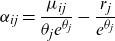 $\alpha_{ij}=\displaystyle\frac{\mu_{ij}}{\theta_j e^{\theta_j}}-\frac{r_j}{e^{\theta_j}}$, then
 \begin{align}p(y_{i1},y_{i2}) =\, & \prod_{j=1}^2 \exp\left\{\left(\frac{\mu_{ij}}{\theta_j e^{\theta_j}}-\frac{r_j}{e^{\theta_j}}\right)(1-e^{\theta_j})-r_j\theta_j\right\}\frac{\theta_j^{y_{ij}}}{y_{ij}!}B_{y_{ij},r_j}\left(\frac{\mu_{ij}}{\theta_j e^{\theta_j}}-\frac{r_j}{e^{\theta_j}}\right)\nonumber\\[4pt]& \times \left[1+\omega\left[\left(e^{-y_{i1}}-\mathbb{E}\left(e^{-Y_{i1}}\right)\right)\left(e^{-y_{i2}}-\mathbb{E}\left(e^{-Y_{i2}}\right) \right)\right]\right],\end{align}
where  $y_{ij}=0,1,2,\dots$,
 $\mathbb{E}(e^{-Y_j})=\exp \{(\frac{r_j}{e^{\theta_j}}-\frac{\mu_{ij}}{\theta_j e^{\theta_j}}) (e^{\theta_j}-e^{\theta_{j} e^{-1}})-r_j\theta_j c \}$ with
 $\theta_j, r_j>0$,
 $c=1-e^{-1}$ and
 $j=1,2$. Here,
 $\omega\in \mathbb{R} $ is the dependency parameter. For ith individual, the correlation coefficient between the marginals is
 \begin{align*}corr(Y_{i1},Y_{i2}) =\, &\omega \prod_{j=1}^2\exp \left\{\left(\frac{r_j}{e^{\theta_j}}-\frac{\mu_{ij}}{\theta_j e^{\theta_j}}\right) \left(e^{\theta_j}-e^{\theta_{j} e^{-1}}\right)-r_j\theta_j c \right\}\\[3pt]& \times \left(\left(\frac{\mu_{ij}}{\theta_j e^{\theta_j}}-\frac{r_j}{e^{\theta_j}}\right)\theta_j\,\left (e^{(\theta_j e^{-1}-1)}-e^{\theta_j}\right)-r_j\theta_j c\right)\\[3pt]&\times \left(\prod_{j=1}^2\left(\frac{\mu_{ij}}{\theta_j e^{\theta_j}}-\frac{r_j}{e^{\theta_j}}\right)\theta_j e^{\theta_j}(1+\theta_j)+r_j\theta_j\right)^{-1/2}.\end{align*}
When  $\omega= 0$, the pair
 $Y_{i1}$ and
 $Y_{i2}$ are independent. When
 $\omega>0$, the
 $Br{\mathcal B} ell$ regression model allows for positive correlation, and when
 $\omega<0$, accounts for negative correlation. The parameter dependency
 $\omega$ for all
 $i=1,\dots,n$ is restricted to the interval
 $[\omega_{i1},\omega_{i2}]$, where the lower limit
 $\omega_{i1}$ and upper limit
 $\omega_{i2}$ are given by the following expressions:
 \begin{align*}\omega_{i1}&=\frac{-1}{\max \left(\mathbb{E}\left(e^{-Y_{i1}}\right)\mathbb{E}\left(e^{-Y_{i2}}\right),\left(1-\mathbb{E}\left(e^{-Y_{i1}}\right)\right)\left(1-\mathbb{E}\left(e^{-Y_{i2}}\right) \right) \right)}, \\[5pt]\omega_{i2}&=\frac{1}{\max \left(\mathbb{E}\left(e^{-Y_{i1}}\right)\left(1-\mathbb{E}\left(e^{-Y_{i2}}\right)\right),\left(1-\mathbb{E}\left(e^{-Y_{i1}}\right) \right)\mathbb{E}\left(e^{-Y_{i2}}\right) \right) }.\end{align*}
Since each interval depends on the individual expectations, the intervals for the parameters  $\omega$ differ for each i; hence, in practice, we need to select the narrowest interval. The log-likelihood function, for this bivariate regression model, is given by
 \begin{align} \ell({\underline \beta}_1,{\underline \beta}_2,r_1,r_2,\theta_1,\theta_2,\omega) =\, & \sum_{i=1}^n\sum_{j=1}^2 \left(\left(\frac{\mu_{ij}}{\theta_j e^{\theta_j}}-\frac{r_j}{e^{\theta_j}}\right)(1-e^{\theta_j})-r_j\theta_j\right)\nonumber\\[4pt]& + \log\theta_j y_{ij} -\log y_{ij} !+ \log B_{y_{ij},r_j}\left(\frac{\mu_{ij}}{\theta_j}-\frac{r_j}{\theta_j}\right)\nonumber\\[4pt]& + \log\left[1+\omega\left[\left(e^{-y_{i1}}-\mathbb{E}\left(e^{-Y_{i1}}\right)\right)\left(e^{-y_{i2}}-\mathbb{E}\left(e^{-Y_{i2}}\right) \right)\right]\right].\nonumber\\[5pt]\end{align}
The function (18) can be directly maximised with respect to the vector of parameters  $({\underline \beta}_1,{\underline \beta}_2,r_1,r_2,\theta_1,\theta_2,\omega)$. We have used different maximum search methods that are available in the FindMaximum built-in function in the Mathematica software package. The asymptotic standard deviations of the estimated parameters are obtained in the usual way from Hessian matrix.
6. Numerical Illustrations
In this section, we will first carry out a simulation analysis to test the performance of the maximum likelihood estimates. Then, by using several motor vehicle datasets, we test the performance of the univariate and bivariate versions of the  $r{\mathcal B}ell$ distribution.
6.1 A simulation analysis
By using the algorithm given in Remark 3, a complete simulation analysis for the  $r{\mathcal B}ell$ distribution is carried out by generating
 $N:=1000$ samples of sizes
 $n:=100,\, 300,\,500$ for different values of the parameters
 $\alpha$, r and
 $\theta$. For each parameter, the analysis computes the following measures:
• Average bias (AB) of the simulated estimates:
$AB(\Lambda^{*})=\displaystyle\frac{1}{N}\sum_{j=1}^{N}(\Lambda_j^{*}-\Lambda)$;-
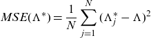
• Mean square error (MSE) of the simulated estimates:
$MSE(\Lambda^{*})=\displaystyle\frac{1}{N}\sum_{j=1}^{N}(\Lambda_j^{*}-\Lambda)^2$,
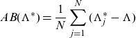
where  $\Lambda_i^{*}$ represents the maximum likelihood estimate of each parameter in the jth sample and
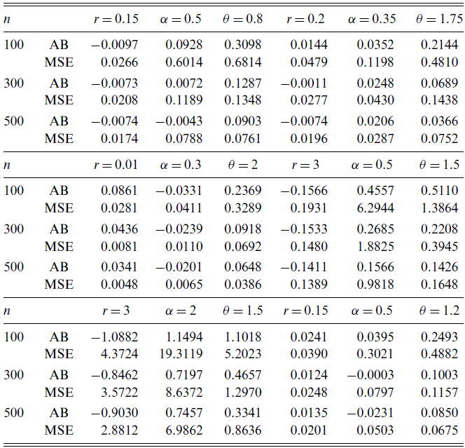
 $\Lambda$ is the true value of the parameter. Table 1 shows the average bias and mean square errors of the parameter estimates for different values of r,
 $\alpha$ and
 $\theta$ for different values of n. We have selected three combinations of parameters for which the PMF is unimodal with mean located at zero, one situation where the PMF tends to be unimodal and symmetric and two other cases showing bimodality. As expected, the mean square error decreases when n increases. It seems that for these values of the sample sizes, the mean square errors of the parameter values increase when the parameters r and
 $\alpha$ grow. However, for the cases
 $\alpha=0.5,\,r=3,\,\theta=1.5$ and
 $\alpha=2,\,r=3,\,\theta=1.5$, we have numerically verified that
 $\displaystyle \lim_{n\to \infty}MSE(\Lambda^{*})=0$, therefore the estimates are consistent in mean square error. It implies that the estimate gets closer and closer to the parameter’s true value as data accumulates. Also, for large values of n, the maximum likelihood estimators are normally distributed with the mean equals to the true value of the parameter and variance equal to the reciprocal of the information function evaluated at the mean.
Average bias (AB) and mean square error (MSE) of the maximum likelihood estimates for different values of the parameters of the
 $r{\mathcal B}ell$
distribution for different samples sizes n with simulation size
 $N:=1000$
.

6.2 Application to motor vehicle insurance data
6.2.1 Case without covariates
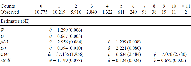
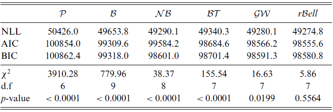
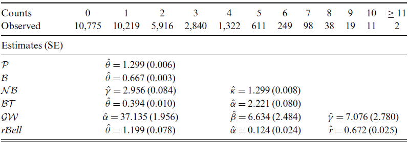
The performance of the  $r{\mathcal B}ell$ distribution is examined by using the French Motor Personal Line datasets available from the package ‘CASdatasets’ in R. This is a collection of 10 datasets from a private motor French insurer. Each dataset includes risk features, claim amount and claim history of around 30,000 policies for 2004. We first consider the set of data freMPL10 that includes 32,100 policies. In this dataset, we are considering the total number of claims by adding the claims in the following variables: <monospace>ClaimNbResp</monospace>, the number of responsible claims in the four preceding years, <monospace>ClaimNbNonResp</monospace> number of non-responsible claims in the four preceding years, <monospace>ClaimNbParking</monospace> number of parking claims in the four preceding years, <monospace>ClaimNbFireTheft</monospace> number of fire–theft claims in the four preceding years, <monospace>ClaimNbWindscreen</monospace> number of windscreen claims in the four preceding years and <monospace>OutUseNb</monospace> number of out-of-use claims in the four preceding years. This dataset is overdispersed since the mean is 1.299, and the sample variance is 1.8934 and the modal value located at 0. It has a moderate–high proportion of zeros (35%) and a long right tail. Total counts and observed frequencies are given in Table 1. Although the time exposures are not the same for all insurance policies, we point out that in this example without covariates, we have assumed that they are equal to one, and therefore offset variables have not been considered in the models considered below.
We have fitted the  $r{\mathcal B}ell$ distribution by using the maximum likelihood method. Parameter estimates and standard errors are given in the last row of Table 1. Note that the condition
 $\theta<(r+\alpha)^{-1}=1.256$ for unimodality at zero is verified.
For comparison purposes, we have fitted the one-parameter Poisson ( $\mathcal P$) and Bell (
 ${\mathcal B}$) distributions, the two-parameter negative binomial (
 ${\mathcal{NB}}$) and Bell–Touchard (
 ${\mathcal{BT}}$) distributions and the three-parameter generalised Waring (
 ${\mathcal{GW}}$) distribution to this dataset. The PMF of
 ${\mathcal{NB}}$ and
 ${\mathcal{GW}}$ are given in the Appendix. We have considered Akaike’s information criterion (AIC) and Bayesian information criterion (BIC) and the negative value of the maximum log-likelihood function (NLL) as comparison criteria. A model with a lower value of these measures of model selection is preferable. As illustrated in Table 2, the
 $r{\mathcal B}ell$ model provides the best fit for this dataset in terms of the three measures of model selection. Although it is not illustrated here, we have also fitted these models together with the Poisson-inverse Gaussian and zero-inflated Poisson (
 ${\mathcal{ZIP}}$) to each separate dataset and the
 $r{\mathcal B}ell$ distribution consistently provides the best fit. Furthermore, the value of the
 $\chi^2$ test statistic for each model considered, the degrees of freedom (DoF) chosen to comply with the rule of five (i.e., expected frequency
 $>5$) and their corresponding p-values are also shown in this table. It is noted that the three-parameter models are not rejected at the 1% significance level, and the
 $r{\mathcal B}ell$ distribution yields the lowest value for the test statistics.
The observed total number of claims in the dataset freMPL10, parameter estimates and standard errors (SE) for all the distributions considered.
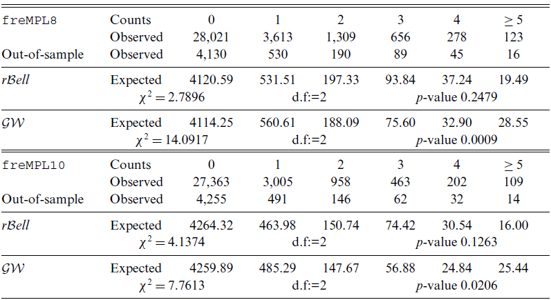
The out-of-sample performance of the  $r{\mathcal B}ell$ distribution is now tested by using the freMPL8 and freMPL10 datasets. In these two datasets, we examine the response variable OutUseNb. Although usually, out-of-use claims arise from accidents that are not directly caused by the vehicle’s driving, a vehicle may be in use when it is stationary, that is the handbrake in a parked car is not properly engaged, and this causes the car to roll and strike a property. These datasets are overdispersed since for the first one the mean is 0.2919 and the variance 0.5700, whereas for the second one, these values are 0.2387 and 0.4714, respectively. Both sets have the modal value at 0. Total counts and observed frequencies for number of out-of-use claims are given in Table 4. These datasets have a high proportion of zeros, 85% and 82%, respectively, and a long right tail. The
 $r{\mathcal B}ell$ distribution provides a better fit to these datasets than the models discussed above. Also, it improves the performance of the
 ${\mathcal{ZIP}}$ distribution. We have randomly partitioned the datasets freMPL8 and freMPL10 into two disjoint subsets of different sizes. The first subset is used for fitting the models, whereas the second subset tests the model’s out-of-sample prediction accuracy. For the freMPL8 dataset we have used 29,000 polices to estimate the model parameters. The remaining 5,000 policies are used to test the model’s out-of-sample prediction accuracy. For the dataset freMPL10 27,100 observations were used to estimate the parameters and 5,000 policies to test the model’s out-of-sample prediction accuracy. We have fitted the
 $r{\mathcal B}ell$ and
 ${\mathcal{GW}}$ distributions to these datasets. The out-of-sample observed and expected frequencies for each model are also illustrated in Table 3. We have compared both models via the chi-square goodness-of-fit test. It is noted that the three-parameter
 $r{\mathcal B}ell$ distribution has better out-of-sample performance since it is not rejected at the usual significance levels. Furthermore, we have also accounted for different time exposures to handle the number of claims per unit of time. For each model, we have considered a linear predictor with two terms, the intercept and the log of the exposure, that is offset variable with a coefficient of 1. For the
 ${\mathcal{GW}}$ distribution, we have reparameterised the shape parameter as
 $\alpha=1+\frac{\gamma \beta}{\mu_i}$ with
 $\mu_{i}=\exp\{\log(\xi_i)+{x_{1i}\beta_1}\}$ where
 $\beta_1$ is the parameter associated to the intercept term. We have fitted both models to the in-sample datasets. In terms of the NLL, the
 ${\mathcal{GW}}$ distribution provides a better fit to data, that is 19829.3 (freMPL8) and 15971.2 (freMPL10), whereas the
 $r{\mathcal B}ell$ distribution yields 20133.1 and 16181.3 for the freMPL8 dataset and freMPL10 dataset, respectively.
Counts and observed frequencies for the NUMBER OF OUT-OF-USE CLAIMS for datasets freMPL8 and freMPL10. Also, out-of-sample observed and expected frequencies and chi-square goodness-of-fit test for the
 $r{\mathcal B}ell$
and
 ${\mathcal{GW}}$
distributions are displayed.

Measures of model selection and chi-square goodness-of-fit test for the different models considered for the total number of claims in the dataset freMPL10.

These two sets of data include several explanatory variables. Descriptions of the most relevant factors and explanatory variables can be found in Table 2 of CalderÍn-Ojeda et al. (Reference CalderÍn-Ojeda, GÓmez-DÉniz and Barranco-Chamorro2019). We have fitted the  $r{\mathcal B}ell$ regression model without accounting for time exposures to these datasets by using the aforementioned random partitions of the datasets freMPL8 and freMPL10. Again, we benchmark the
 $r{\mathcal B}ell$ regression model with other traditionally used regression models in the literature, such as the negative binomial (
 ${\mathcal{NB}}$) and Poisson-inverse Gaussian (
 ${\mathcal{PIG}}$) regression models. Also, the three nested regression models, that is Bell (
 ${\mathcal B}$), Bell–Touchard, (
 ${\mathcal{BT}}$) and Poisson (
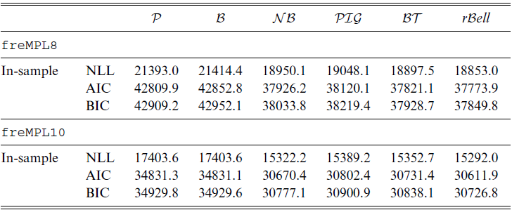
 ${\mathcal P}$) are compared with the model introduced in this work by using the same measures of model selection discussed in the previous example. It is observed from in Table 5 that the
 $r{\mathcal B}ell$ regression model provides the best fit in-sample in terms of the three-model validation measures. It also improves the zero-inflated Poisson regression model for both datasets (see Lee (Reference Lee2021) for a recent reference on this model). Moreover, using the likelihood ratio test, the
 $r{\mathcal B}ell$ regression model is preferable to all nested regression models, in-sample and out-of-sample for both datasets, as judged by the corresponding p-values. When comparing the regression model introduced in this paper with the
 ${\mathcal P}$,
 ${\mathcal B}$ and
 ${\mathcal{BT}}$ ones for both datasets, those p-values are always less than
 $0.01$.
Measures of model selection (in-sample) for different regression models considered for the number of claims in the freMPL8 and freMPL10 datasets.

Finally, we compare  $r{\mathcal B}ell$ regression model with the
 ${\mathcal{NB}}$ and
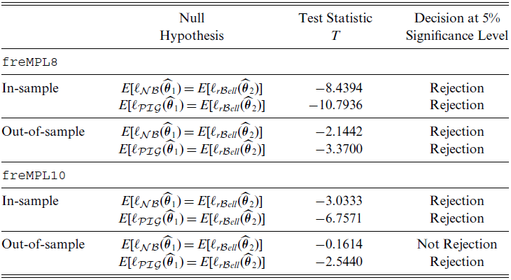
 ${\mathcal{PIG}}$ regression models and analyse the model selection through the likelihood ratio test proposed by Vuong (Reference Vuong1989) for non-nested models. The test statistic of Vuong’s closeness test is
 \begin{eqnarray*}T=\frac{1}{\omega\sqrt{n}}\left(\ell_{f}(\widehat{\boldsymbol{\theta}}_1)-\ell_{g}(\widehat{\boldsymbol{\theta}}_2)-\log n\left(\frac{n_f}{2}-\frac{n_g}{2}\right)\right),\,\,\text{where}\\{\omega^2=\frac{1}{n}\sum_{i=1}^{n}\left[\log\left(\frac{f(y_i|\widehat{\boldsymbol{\theta}}_1)}{g(y_i|\widehat{\boldsymbol{\theta}}_2)}\right)\right]^2-\left[\frac{1}{n}\sum_{i=1}^{n}\log\left(\frac{f(y_i|\widehat{\boldsymbol{\theta}}_1)}{g(y_i|\widehat{\boldsymbol{\theta}}_2)}\right)\right]^2}\end{eqnarray*}
is the sample variance of the pointwise log-likelihood ratios and  $f(\cdot)$ and
 $g(\cdot)$ represent the PMF of two different non-nested models,
 $\widehat{\boldsymbol{\theta}}_1$ and
 $\widehat{\boldsymbol{\theta}}_2$ are the maximum likelihood estimates of
 ${\boldsymbol{\theta}}_1$ and
 ${\boldsymbol{\theta}}_2$ and
 $n_f$ and
 $n_g$ are the number of estimated parameters in the model with PMF
 $f(\cdot)$ and
 $g(\cdot)$, respectively. Note that the Vuong’s statistic is sensitive to the number of estimated parameters in each model and therefore the test must be corrected for dimensionality. We test
 $H_0:E[\ell_{f}(\widehat{\boldsymbol{\theta}}_1)-\ell_{g}(\widehat{\boldsymbol{\theta}}_2)]=0$ against
 $H_0:E[\ell_{f}(\widehat{\boldsymbol{\theta}}_1)-\ell_{g}(\widehat{\boldsymbol{\theta}}_2)] \neq 0$. Under the null hypothesis, T is asymptotically normally distributed. At the 5% significance level, the rejection region for this test in favour of the alternative hypothesis occurs when
 $|T|>1.96$. Table 5 shows the null hypothesis, test statistics and decision at the 5% significance level for each comparison. It is observable that
 $r{\mathcal B}ell$ regression model is preferable to the
 ${\mathcal{PIG}}$ and
 ${\mathcal{NB}}$ regression models at the 5% significance level, in-sample and out-of-sample for the freMPL8 dataset. Also, it is preferable to both models at the same nominal level in-sample and the
 ${\mathcal{PIG}}$ regression model out-of-sample for the freMPL10 dataset.
6.3 Bivariate case
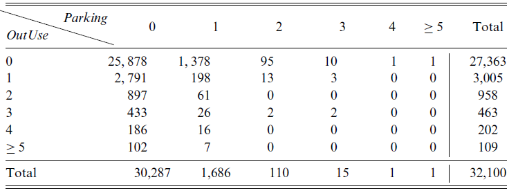
We now explore the relationship between the response variables number of out-of-use claims (OutUse) and number of parking claims (Parking) in the four preceding years, both included in the <monospace>freMPL10</monspace> dataset. At first sight, it seems that these variables are positively correlated; however, we observe that the correlation is positive but very weak by computing the sample correlation coefficient, that is 0.0164. The bivariate empirical distribution also has a high frequency of common zeros, a moderate-size right tail. Mean and sample variance of number of out-of-use claims are 0.2387 and 0.4714, whereas the corresponding figures for number of parking claims are 0.0611 and 0.0680, respectively. In Table 6, empirical frequencies are shown. We have fitted the  $Br{\mathcal B}ell$ regression model to this bivariate dataset. The maximum likelihood estimates and the corresponding standard errors (SE) are exhibited in Table 7. It is observable that only the explanatory variables PRIVATE+, and HASKMLIMIT, are statistically significant at the 5% significance level for both response variables. In addition to this, the estimate of the parameter INTERCEPT,
 $\theta_j$ for
 $j=1,2$ and the dependency parameter
 $\omega$ are also statistically significant at the same nominal level. Finally, for each sample observation it was computationally checked that the estimate of the dependency parameter
 $\hat \omega$ falls into the interval
 $[\omega_{i1},\omega_{i2}]$ with
 $i=1,\dots, 32100$. To show that the model accounts for an excess of zeros, we have conducted a chi-squared goodness-of-fit test to check that in the empirical data without covariates, under the null hypothesis, the bivariate
 $Br{\mathcal B}ell$ distribution adheres well to the bivariate empirical distribution. To comply with the rule of five, we combined the cells in 11 different groups. Then, by assuming that the theoretical distribution of the test statistics is
 $\chi^{2}_{3}$, based on the p-value, that is 0.6464, there is no empirical evidence to reject the
 ${B}r{\mathcal B}ell$ distribution to model this bivariate dataset. Besides, we compared the distribution with the zero-inflated bivariate Poisson distribution in Li et al. (Reference Li, Lu, Park, Kiim, Brinkley and Peterson1999). For this model, we implemented a separate MLE method iterated till convergence. In terms of NLL criterion, the
 $Br{\mathcal B}ell$ distribution provides 25982.8, whereas the bivariate ZIP yields 26779.2.
Null hypothesis, test statistic and decision for Vuong’s test (in-sample and out-of-sample) for freMPL8 and freMPL10 datasets.

Observed frequencies of NUMBER OF OUT-OF-USE CLAIMS and NUMBER OF PARKING CLAIMS in the four preceding years.

For comparison purposes, we have also fitted to this dataset all the nested regression models, that is the bivariate Poisson ( $B{\mathcal P}$), bivariate Bell (
 $B{\mathcal B}$), bivariate Bell–Touchard (
 $B{\mathcal{BT}}$) together with the bivariate negative binomial (
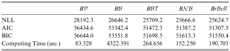
 $B{\mathcal{NB}}$) regression models. Again we compute the AIC and BIC, and NLL to compare the models. Results are shown in Table 9. It is discernible that the
 $Br{\mathcal B}ell$ regression model provides the best fit for the three measures of model selection. The computing times in seconds are also displayed in the last row of this table. The computations were performed on a computer with Intel(R) Core(TM)i7-6700CPU@3.40GHz 16GB RAM by using Wolfram Mathematica 12.0 software package.
Measures of model selection for different bivariate regression models are considered.

7. Conclusions and Extensions
In this paper, we have introduced a three-parameter family of discrete distributions, which is based on the series expansion of the r-Bell polynomials, named as the  $r{\mathcal B}ell$ distribution. This family of distributions enjoys interesting stochastic properties. It is a special case of the multiple Poisson process. Moreover, its probability mass function can be either unimodal or bimodal. It has a zero vertex for small values of parameter
 $\theta$, it is overdispersed, and its probabilities can be computed by a recursive formula that allows us to calculate the probability function of the amount of aggregate claims in the collective risk model in terms of an integral equation. This model nests as particular cases the Poisson distribution and the recently proposed Bell and Bell–Touchard distributions. Furthermore, univariate and bivariate regression models based on this discrete family of distributions were implemented. The latter regression model was derived via the Sarmanov distribution, allowing for positive or negative correlation. It can describe the model dependency in bivariate settings with given marginals. These regression models were used to explain the number of out-of-use and parking claims in an automobile insurance portfolio, by showing a good out-of-sample performance. Therefore, this family of distribution is a useful alternative to other traditionally used models to explain count data such as the negative binomial and Poisson-inverse Gaussian distributions.
On the other hand, it would be interesting to investigate the relationship of the proposed model with the convolution of a Neyman Type A distribution with a Poisson distribution (see Kemp (Reference Kemp1967)) and further explore actuarial properties of this more general model. This family of distributions might be extended to a multivariate regression model based on the trivariate Sarmanov distribution similar to the models derived in BolancÉ and Vernic (Reference BolancÉ and Vernic2019). This model could be used to explain situations where the policyholder has purchased policies in different insurance lines or in cases where the insured wishes to extend the third-party motor vehicle insurance to account for different coverages that adapt to their personal needs. Alternatively, it could be possible to implement a multivariate version with elliptical copula-based models to accommodate a wide range of dependence. It is important to point out that the properties of the copula are not the same as for continuous random variables since the probability of ties in the data are positive. Thus, the estimation cannot be directly carried out, and a continuous extension of integer-valued random variables is needed by using the approach proposed by Denuit and Lambert (2005).
Acknowledegments
The authors would thank Prof. Miloud Mihoubi, Faculty of Mathematics, USTHB, Algeria, for his comments and discussion on the proof of Theorem 1 and and Dr Violetta Piperigou Violetta, University of Patras, for bringing to our attention some important references. We are also grateful to the editor and all four anonymous referees for their constructive comments and suggestions, which have greatly helped us improve the manuscript.
Supplementary material
To view supplementary material for this article, please visit http://dx.doi.org/10.1017/asb.2021.14.
A. Appendix
• PMF of the negative binomial distribution
\begin{equation*}f(y|\kappa,\gamma)=\frac{\Gamma(y+\gamma)}{\Gamma(y)\Gamma(\gamma)}\left(\frac{\kappa}{\gamma+\kappa}\right)^y\left(\frac{\gamma}{\gamma+\kappa}\right)^\gamma,\,\;y=0,1,2,\dots\,\gamma,\kappa>0. \end{equation*}
-
• PMF of the generalised Waring distribution
\begin{equation*}f(y|\alpha,\beta,\gamma)=\frac{\Gamma(y+\gamma)}{\Gamma(y)\Gamma(\gamma)}\frac{Be(\alpha+\gamma,\beta+y)}{Be(\alpha,\beta)},\,\;y=0,1,2,\dots\,\alpha,\beta,\gamma>0. \end{equation*}


Proof of Proposition 1. The recurrence relation of the r-Bell polynomials, see Theorem 4.2 of MezÖ (Reference MezÖ2011), is given by
 \begin{equation} B_{y,r}(\alpha)= rB_{y-1,r}(\alpha)+ \alpha \sum_{k=0}^{y-1}\binom{y-1}{k}B_{k,r}(\alpha).\end{equation}
By multiplying 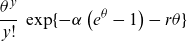 $\displaystyle\frac{\theta^y}{y!}\,\exp\{-\alpha \left(e^\theta -1\right)-r\theta\}$ both sides of (19) and after some algebra, we obtain
 \begin{equation} p_Y(y)=\frac{r \theta}{y} p_Y(y-1) +\frac{\alpha \theta}{y} \sum_{k=0}^{y-1}\frac{\theta^{y-k-1}}{(y-k-1)!} p_Y(k) \quad y=1,2,\dots\end{equation}
with  $p_Y(0)=\exp\{-\alpha \left(e^\theta -1\right)-r\theta\}$.
 $\blacksquare$
Lemma A.1. The sequence 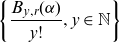 $\left\lbrace \displaystyle\frac{B_{y,r}(\alpha)}{y!}, y \in \mathbb{N}\right \rbrace$, is log-concave for either
 $(0<\alpha<1) \cap (\sqrt{\alpha}-\alpha<r<\alpha)$ or
 $(\alpha>1 \cap r>0)$.
Proof of Lemma A.1. For  $\alpha>0$, let
 $c_y(\alpha)=\frac{B_{y,r}(\alpha)}{y!}$, where
 $B_{y,r}(\alpha)$ are the r-Bell polynomials defined in (4). The generating function of
 $c_y(\alpha)$ is
 \begin{align*}\sum_{y=0}^{\infty} c_y(\alpha) u^y=& \sum_{y=0}^{\infty} \frac{B_{y,r}(\alpha)}{y!} u^y= e^{-\alpha}\sum_{y=0}^{\infty}\sum_{k=0}^{\infty} \frac{(k+r)^y}{k!}\frac{u^y}{y!}\alpha^k = \exp\{\alpha(e^u-1)+ur\}.\end{align*}
Note that  $\exp\{\alpha(e^u-1)+ur\}=\exp\lbrace\sum_{j=1}^{\infty}\frac{Z_j}{j}u^j\rbrace$, where
 $Z_1= \alpha+r$ and
 $Z_j=\frac{\alpha}{(j-1)!}$ for
 $j \ge 2$. It is easy to check that the sequence
 $1,Z_1,Z_2,\dots$ is log-concave for either
 $\left((0<\alpha<1)\cap (\sqrt{\alpha}-\alpha<r<\alpha)\right)$ or
 $\left(\alpha>1 \cap r>0\right)$. Hence, the log-concavity of
 $c_y(\alpha)$ follows from Theorem 1 in Bender and Canfield (Reference Bender and Canfield1996), which states that if the sequence
 $1,Z_1,Z_2,\dots$ is non-negative and log-concave, then so is the sequence
 $1,c_1(\alpha),c_2(\alpha),\dots$ determined by the generating function equation
 $\sum_{y \ge 0} {c_y(\alpha)} u^y = \exp \left\lbrace \sum_{j\ge 1} \frac{Z_ju^j}{j} \right\rbrace.$
 $\blacksquare$
Proof of Proposition 2. Since by Lemma 1 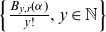 $\left\lbrace \frac{B_{y,r}(\alpha)}{y!}, y \in \mathbb{N} \right\rbrace$ is log-concave for
 $(0<\alpha<1) \cap (\sqrt{\alpha}-\alpha<r<\alpha)$ or
 $\left(\alpha>1 \cap r>0\right)$, we have that
 $\left(\frac{B_{y+1,r}(\alpha)}{(y+1)!}\right)^2 \ge \frac{B_{y,r}(\alpha)}{y!} \frac{B_{y+2,r}(\alpha)}{(y+2)!} .$ Hence, the PMF
 $p_y=\exp \left\{-\alpha \left(e^\theta -1\right)-r\theta\right\} \frac{\theta^y}{y!}B_{y,r}(\alpha)$ forms a log-concave sequence
 $\{p_y,y=0,1,2,\dots\}$ for either
 $(0<\alpha<1) \cap (\sqrt{\alpha}-\alpha<r<\alpha)$ or
 $\left(\alpha>1 \cap r>0\right)$, which satisfies the necessary and sufficient condition for strong unimodality. Hence, the result follows by using Theorem 3 in Keilson and Gerber (Reference Keilson and Gerber1971).
 $\blacksquare$
Proof of Proposition 3. This can be obtained by solving the set of equations  $p_Y(1)/p_y(0)<1$ and
 $p_Y(2)/p_y(1)<1$ simultaneously, for
 $(0<r<\sqrt{\alpha}-\alpha) \cap (0<\alpha<1)$.
 $\blacksquare$
Proof of Theorem 1. For  $\theta>0$, plugging
 $c_1=(\alpha+r)\theta$,
 $c_n=\displaystyle\frac{\alpha \theta^n}{n!}$
 $n\geq 2$ and
 $t=1$ into (9), yields
 \begin{eqnarray} W_k(1)&=& \exp\left\lbrace-(\alpha+r)\theta-\alpha\sum_{n=0}^{\infty} \frac{\theta^n}{n!} \right\rbrace \sum_{s_1+2s_2+\dots+k s_k=k}\frac{((\alpha+r)\theta)^{s_1}(\alpha \theta^2)^{s_2}\dots(\alpha \theta^k )^{s_k}}{s_1!s_2!\dots s_k! (1!)^{s_1} (2!)^{s_2}...(k!)^{s_k}} \nonumber \\ &=&\exp\left\lbrace-\alpha \left(e^\theta-1\right) -r\theta \right\rbrace\frac{1}{k!} \phi_k, \end{eqnarray}
where  $\phi_k=\sum_{s_1+2s_2+\dots+k s_k=k}\frac{k!((\alpha+r)\theta)^{s_1}(\alpha \theta^2)^{s_2}\dots(\alpha \theta^k )^{s_k}}{s_1!s_2!\dots s_k! (1!)^{s_1} (2!)^{s_2}...(k!)^{s_k}}$. Further, the exponential generating function for the sequence
 $\lbrace \phi_k\rbrace_{k>0}$ is given by
 \begin{align*}\sum_{k \ge 0}\phi_k\frac{t^k}{k!} =& \sum_{k \ge 0} \left(\sum_{s_1+2s_2+\dots+k s_k=k}\frac{k!((\alpha+r)\theta)^{s_1}(\alpha \theta^2)^{s_2}\dots(\alpha \theta^k )^{s_k}}{s_1!s_2!\dots s_k! (1!)^{s_1} (2!)^{s_2}...(k!)^{s_k}}\right) \frac{t^k}{k!}\\=& \sum_{{s_i \ge 0,\,i=1,2,\dots}} \frac{1}{s_1! s_2!\dots}\left(\frac{(\alpha+r)\theta t}{1!} \right)^{s_1}\left(\frac{\alpha(\theta t)^2}{2!} \right)^{s_2}\dots\left(\frac{\alpha (\theta t)^k}{k!} \right)^{s_k} \dots \\=&\exp\left\lbrace r \theta t +\alpha \sum_{j\ge 1}\frac{(\theta t)^j}{j!} \right\rbrace = \exp \left \lbrace r\theta t +\alpha (e^{\theta t}-1)\right\rbrace =\sum_{k \ge 0} B_{k,r}(\alpha) \frac{(\theta t)^k}{k!}.\end{align*}
Hence comparing the coefficients of  $t^k$, we get
 $\phi_k= \theta^k B_{k,r}(\alpha)$. Substituting the latter expression in (21), we get the desired result.
 $\blacksquare$
Proof of Proposition 4. The result follows from the r-Bell expansion defined in  $(3)$, that is,
 \begin{eqnarray*}G_Y(s)&=&\mathbb{E}(s^Y)= \sum_{y=0}^{\infty}s^y \exp \left\{-\alpha \left(e^\theta -1\right)-r\theta\right\} \frac{\theta^y}{y!}B_{y,r}(\alpha) \\&=&\exp\left\{-\alpha \left(e^\theta -1\right)-r\theta\right\}\exp\left\{\alpha \left(e^{s \theta } -1\right)+r s\theta\right\}\\&=&\exp\left\{\alpha\left(e^{s\theta}-e^{\theta}\right)+r\theta(s-1)\right\}, \,|s|<1.\\[-34pt]\end{eqnarray*}
 $\blacksquare$
Proof of Proposition 5. The result follows immediately since (10) can be written as
 \begin{align*}G_Y(s)=\mathbb{E}(s^Y)&=\exp\left\{\alpha\left(e^{s\theta}-e^{\theta}\right)\right\}\,\exp\left\{r\theta(s-1)\right\}=G_{X}(s)\,G_{Z}(s), \quad |s|<1.\\[-35pt]\end{align*}
 $\blacksquare$
Proof of Proposition 6. It is straightforward by using  $G_{Y_{1}+\dots+Y_{n}}(s)=G_{Y_{1}}(s)\dots G_{Y_{n}}(s)$.
 $\blacksquare$
Proof of Proposition 7. The result follows after simple algebra by using the definition of CGF.  $\blacksquare$
Proof of Result 1. The MGF of the Esscher transform of Y with parameter  $t>0$, is
 $M_E(t)=\exp\left\{\alpha\left(e^{e^t\theta e^{h}}-e^{\theta e^{h}}\right)+r\theta e^{h}(e^t-1)\right\}.$ Then, the result follows by evaluating
 $M'_{E}(t)_{|t=0}$.
 $\blacksquare$
Proof of Result 2. By taking into consideration that the Esscher transform of X, that is  $\check X$, is given by
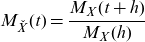 $M_{\check X}(t)=\displaystyle\frac{M_X(t+h)}{M_X(h)}$, then the MGF of
 $\check S$ is
 \begin{equation*}M_{\check S}=\frac{M_S(t+h)}{M_S(h)}=\exp\left\{\alpha\left(e^{\check\theta M_{\check X}(t)}-e^{\check\theta }\right)+r\check\theta (M_{\check X}(t)-1)\right\}.\end{equation*}
Then, the result follows by evaluating  $M'_{\check S}(t)_{|t=0}$.
 $\blacksquare$
Proof of Lemma 3. By rewriting (4) as  $B_{y,r}(\alpha)= e^{-\alpha} \sum_{k=0}^{\infty}(k+r) \frac{(k+r)^{y-1}}{k!} \alpha^{k}$ and after computation we get,
 $B_{y,r}(\alpha)=\alpha B_{y-1,r+1}(\alpha)+rB_{y-1,r}(\alpha).$ Then, multiplying both sides of above equation by
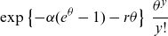 $\displaystyle \exp\left\{-\alpha(e^\theta-1)-r\theta\right\}\,\frac{\theta^y}{y!}$ and after simplification we obtain the required result.
 $\blacksquare$
Proof of Theorem 2. When F(x) is a absolutely continuous distribution with  $F(0) = 0$, the aggregate claims distribution S has a mixed distribution with PDF
 $f_S(x)=\sum_{k=1}^{\infty} p(k;r,\alpha,\theta) f^{k \ast}(x)$ for
 $x > 0$, and with a mass of probability at 0, that is
 $p(0;r,\alpha,\theta)$, where
 $f^{k\ast}(x)$ denotes the k-fold convolution of f(x). Now, using (14), we have
 \begin{align*}\sum_{k=1}^{\infty} p_Y(k;r,\alpha,\theta) f^{k\ast}(x) = & \alpha \theta e^{-\theta} \sum_{k=1}^{\infty} \frac{1}{k} p_Y(k-1;r+1,\alpha,\theta) f^{k \ast}(x)\\[4pt]& + r\theta \sum_{k=1}^{\infty} \frac{1}{k} p_Y(k-1;r,\alpha,\theta) f^{k \ast}(x).\end{align*}
Now, by using the identity,  $\displaystyle\frac{f^{k \ast}(x)}{k}=\int_{0}^{x}\frac{y}{x} f^{(k-1)\ast}(x-y)f(y)dy, \quad k=1,2,\dots,$ and after some simple calculations we obtain the result.
 $\blacksquare$
Parameter estimates and standard errors for
 $Br{\mathcal B}ell$
regression model by using the response variables in Table 2 of CalderÍn-Ojeda et al. (Reference CalderÍn-Ojeda, GÓmez-DÉniz and Barranco-Chamorro2019).