





Impact Statement
Inspired by the tubercle structures on the pectoral flippers of humpback whales, the sinusoidal leading-edge modification to an aerofoil has demonstrated advantages in softening the onset of stall. By combining high-speed three-dimensional particle tracking, physics-informed neural network data assimilation and proper orthogonal decomposition, we are able to resolve the volumetric velocity and pressure fields around an aerofoil with leading-edge tubercles under the attached and separated flow conditions, capturing the formation of spanwise-periodic vortices at low angles of attack and large-scale, unsteady separation cells in the post-stall regime. The detailed characterisation of the vortical structures offers insight for the design of aerofoil modifications to improve the stall behaviour where a more stable lift output with increasing angle of attack is preferred. The results from this study are particularly relevant to moderate- to low-Reynolds-number applications, such as micro-aerial vehicles, small rotors, vertical axis wind turbines and compact hydro energy harvesting.
1. Introduction
The sinusoidal leading-edge modification to a wing or blade is inspired by the tubercle structures on the pectoral flippers of humpback whales (Fish et al. Reference Fish, Weber, Murray and Howle2005). These structures are believed to enhance their swimming by enabling a smaller turning radius during highly dynamic manoeuvres (Fish Reference Fish1999). Leading-edge tubercles have been shown to improve the performance of three-dimensional (3-D) flippers by increasing the maximum lift and postponing the onset of stall, where the lift coefficient begins to decrease as the angle of attack (denoted by
 $\alpha$
) is increased further (Miklosovic et al. Reference Miklosovic, Murray, Howle and Fish2004; Carreira Pedro & Kobayashi Reference Carreira Pedro and Kobayashi2008). The effect of tubercles has also been studied on two-dimensional (2-D) aerofoils (Johari et al. Reference Johari, Henoch, Custodio and Levshin2007; Miklosovic et al. Reference Miklosovic, Murray and Howle2007; Hansen et al. Reference Hansen, Kelso and Dally2011; Valls Badia et al. Reference Valls Badia, Hickel, Scarano and Li2025), and the main advantage of tubercles is found in the post-stall condition, where a 50 % increase in the lift has been reported with limited drag penalty, but stall onset occurs at a lower
 $\alpha$
and the maximum attainable lift is lower compared with the aerofoil with a straight leading edge (Johari et al. Reference Johari, Henoch, Custodio and Levshin2007).
Although tubercles on the flipper of humpback whales have an irregular distribution, most aerodynamic studies of tubercled aerofoils have been performed adopting a simplified, more regular geometry, where the leading edge of the aerofoil is varied sinusoidally. The two main parameters characterising such geometry are the tubercle amplitude
 $A$
, defined as half the chordwise distance between peak and trough, and the spanwise wavelength
 $\lambda$
, defined as the distance between two peaks. A schematic of
 $A$
and
 $\lambda$
is shown in figure 1(b). Normalisation by the mean chord length
 $c_0$
yields the non-dimensional parameters
 $A^*$
and
 $\lambda ^*$
, respectively. Previous studies have explored the effect of
 $A^*$
(approximately in [0.01, 0.1]) and
 $\lambda ^*$
(approximately in [0.1, 1]) on the aerodynamic properties of aerofoils and wings. Relevant works from literature are summarised in supplementary table 1. The general consensus on the effect of tubercle size is that, for a larger tubercle amplitude, a lower maximum lift coefficient (
 $C_{L,\text{max}}$
) is reached at a smaller
 $\alpha$
, and decrease in aerodynamic lift is more gradual in the post-stall regime (Johari et al. Reference Johari, Henoch, Custodio and Levshin2007; Hansen et al. Reference Hansen, Kelso and Dally2011).
Several hypotheses have been formed to explain the favourable post-stall effect of leading-edge tubercles, as critically reviewed by Bolzon et al. (Reference Bolzon, Kelso and Arjomandi2016). The most widely invoked is that the streamwise vortex pairs produced by the tubercles enhance mixing across the boundary layer, which delays separation (Johari et al. Reference Johari, Henoch, Custodio and Levshin2007; Carreira Pedro & Kobayashi Reference Carreira Pedro and Kobayashi2008; Cai et al. Reference Cai, Zuo, Maeda, Kamada, Li, Shimamoto and Liu2017). This mechanism is similar to the effect of an array of vortex generators (Miklosovic et al. Reference Miklosovic, Murray, Howle and Fish2004; Hansen et al. Reference Hansen, Kelso and Dally2011; Zhang et al. Reference Zhang, Wang and Xu2014). In the post-stall regime, the tubercles compartmentalise the separated flow, which inhibits spanwise communication with a mechanism similar to that of wing fences. As a result, regions of reversed flow are separated and locally confined, exhibiting a weaker spanwise momentum exchange (Cai et al. Reference Cai, Zuo, Maeda, Kamada, Li, Shimamoto and Liu2017, Reference Cai, Zuo, Morimoto, Maeda, Kamada and Liu2018). The latter mechanism is believed to play a key role in reducing leading-edge separation at the tip of 3-D flippers, where the small chord length corresponds to a relatively low Reynolds number (Miklosovic et al. Reference Miklosovic, Murray and Howle2007; Carreira Pedro & Kobayashi Reference Carreira Pedro and Kobayashi2008; Moscato et al. Reference Moscato, Mohamed and Romano2022). Other mechanisms, such as vortex lift generated by the streamwise vortices (Moscato et al. Reference Moscato, Mohamed and Romano2022) and the greater distance for pressure recovery behind the troughs (van Nierop et al. Reference van Nierop, Alben and Brenner2008), have been hypothesised, which are less likely to account for the performance of leading-edge tubercles (Bolzon et al. Reference Bolzon, Kelso and Arjomandi2016). It is worth noting that these mechanisms are not mutually exclusive and may co-exist in real-world scenarios.
At small
 $\alpha$
, the structure of the streamwise vortex pairs generated by the tubercles has been relatively well characterised with flow visualisation experiments (Custodio Reference Custodio2007; Hansen et al. Reference Hansen, Kelso and Dally2011) and quantified with particle image velocimetry (PIV) (Custodio Reference Custodio2007; Wei et al. Reference Wei, New and Cui2015) and computational fluid dynamics (Dropkin et al. Reference Dropkin, Custodio, Henoch and Johari2012; Rostamzadeh et al. Reference Rostamzadeh, Hansen, Kelso and Dally2014; Cai et al. Reference Cai, Zuo, Maeda, Kamada, Li, Shimamoto and Liu2017). Behind the tubercle peak, a pair of counter-rotating streamwise vortices is formed, which induces a downwash behind the peak and upwash at the trough. The pattern is similar to that observed above a delta wing at incidence, except that the streamwise vortices produced by tubercles propagate in a rectilinear fashion rather than conical for the delta wing. The downwash motion locally delays boundary layer separation over the aerofoil. Conversely, at the trough, the upwash motion promotes earlier flow separation. Increasing
 $\alpha$
up to the near- and post-stall regimes, larger aperiodic separated regions emerge from the reversed flow region, spanning several wavelengths and involving multiple vortex pairs (Johari et al. Reference Johari, Henoch, Custodio and Levshin2007; Dropkin et al. Reference Dropkin, Custodio, Henoch and Johari2012; Cai et al. Reference Cai, Zuo, Maeda, Kamada, Li, Shimamoto and Liu2017). Due to their finite spanwise extent, the flow organisation within these regions features two quasi wall-parallel recirculatory structures producing ‘mushroom’ or ‘owl-face’ patterns revealed by surface shear stress lines (Hansen et al. Reference Hansen, Rostamzadeh, Kelso and Dally2016; Cai et al. Reference Cai, Zuo, Maeda, Kamada, Li, Shimamoto and Liu2017) or oil flow visualisation, which are similar to the stall cells observed on 2-D aerofoils with a straight leading edge (Winkelmann et al. Reference Winkelmann, Barlow, Saini, Anderson and Jones1980; Weihs & Katz Reference Weihs and Katz1983; Yon & Katz Reference Yon and Katz1998; Dell’Orso & Amitay Reference Dell’Orso and Amitay2018). On a tubercled aerofoil, the stall-cell structures tend to be centred behind the troughs and their size appears to be modulated by the tubercle wavelength. However, the absolute size of these separated regions, their formation mechanism and the aperiodic behaviour are yet to be understood. Moreover, most of existing works focus on the time-averaged properties, while the unsteady behaviour of these cellular structures remained largely unexplored, despite its importance for time-dependent loads and applications.
The present work elucidates the stalling process of tubercled aerofoils by visualising the 3-D interaction between streamwise vortices and stall cells using 3-D time-resolved particle tracking velocimetry (PTV), or Lagrangian particle tracking. The set-up of experiments allows simultaneous observation of streamwise and spanwise modes alongside their temporal evolution, which have not been fully investigated in previous studies. Physics-informed neural networks (PINNs) are utilised to assimilate scattered instantaneous velocity data on a Cartesian grid, and to supplement pressure estimation from velocity fields. The work also makes use of space-only proper orthogonal decomposition (POD) (Berkooz et al. Reference Berkooz, Holmes and Lumley1993) applied to velocity fluctuations for the purpose of distilling the dominant large-scale dynamical features of the flow unsteadiness. The spectral analysis corroborates the spatial decomposition to yield a picture of the underlying dynamical flow system. Furthermore, the study provides insight into the intrinsic topology of the streamwise vortices and their interaction with the stall cells. Ultimately, a connection between these flow structures and aerodynamic performance of tubercled aerofoils is attempted, with the aim of advancing separation control and lift hysteresis reduction for engineering applications.
2. Methods
2.1. Flow facility and aerofoil model
The experiments are conducted in the W-Tunnel of the Aerodynamics Laboratory at TU Delft, an atmospheric open-return wind tunnel. The test section is 1.2 m long with a constant cross-section of
 $0.6 \times 0.6 \text{ m}^2$
. The tunnel is operated at a free-stream velocity
 $U_{\infty }=5 \text{ ms}^{-1}$
, with the free-stream turbulence level of approximately 1%, similar to the experimental conditions of Hansen et al. (Reference Hansen, Kelso and Dally2011) and Wei et al. (Reference Wei, New and Cui2015). A symmetric NACA0021 aerofoil is selected as the baseline geometry, a common choice in previous investigations (Hansen et al. Reference Hansen, Kelso and Dally2011; Skillen et al. Reference Skillen, Revell, Favier, Pinelli and Piomelli2013; Rostamzadeh et al. Reference Rostamzadeh, Hansen, Kelso and Dally2014; Pérez-Torró & Kim Reference Pérez-Torró and Kim2017). As illustrated in figure 1(b), the mean chord length of the aerofoil profile is
 $c_0=0.1\,\mathrm{m}$
. The spanwise length of the aerofoil is 0.6 m, corresponding to the full width of the test section, resulting in an aspect ratio of
 $AR=6$
. The mean-chord-based Reynolds number is
 $Re=3.3\times 10^4$
at the chosen free-stream velocity. The model is installed vertically,
 $0.9\,\mathrm{m}$
downstream of the end of the contraction and in the mid-plane of the working section, fixed by two pins at the quarter-chord point. The aerofoil model is rotated to cover the range of incidence
 $\alpha =[0^{\circ },\,5^{\circ },\,\ldots ,\,30^{\circ }]$
. The angular uncertainty is estimated to be within
 $0.5^{\circ }$
. The coordinate system is fixed relative to the laboratory reference frame and remains independent of the aerofoil’s position. As shown in figure 1(a),
 $x$
and
 $y$
represent the streamwise and spanwise directions, respectively, and
 $z$
is perpendicular to both
 $x$
and
 $y$
, forming a right-handed Cartesian coordinate system. The origin is placed at the nose of baseline aerofoil at the
 $\alpha = 0^{\circ }$
position, with
 $y=0$
at the midspan.
(a) Experimental arrangement in the W-Tunnel and 3-D-PTV system layout. (b-i) Top view of the aerofoil model, with definitions of wavelength
 $\lambda$
and amplitude
 $A$
illustrated. (b-ii) Peak, trough and baseline aerofoil profiles of case
 $A^*=0.1$
positioned at
 $\alpha = 0^{\circ }$
. (c-i) Three-dimensional view and (c-ii) side view of the distribution of particle tracks,
 $A^*=0.1$
at
 $\alpha = 15^{\circ }$
. The particle track length displayed is 10 frames.

Figure 1 Long description
Panel A: A schematic of the experimental arrangement in a wind tunnel showing a wing model, measurement volume, knife-edge filter, LED array, and high-speed cameras. Panel B-i: Top view of the aerofoil model with definitions of wavelength and amplitude. Panel B-ii: Aerofoil profiles showing peak, trough, and baseline positions. Panel C-i: Three-dimensional view of particle tracks distribution. Panel C-ii: Side view of particle tracks distribution.
The leading edge of the tubercled aerofoil is modelled as a sinusoidal variation along the spanwise coordinate
 $y$
with amplitude
 $A$
and wavelength
 $\lambda$
. The resulting spanwise chord length variation is
 \begin{equation} c(y) = c_0+A\sin \left (2\pi y/\lambda -\pi /2\right )\!, \end{equation}
where the phase shift
 $\pi /2$
is to ensure that the origin of the
 $y\hbox{-}$
axis corresponds to a trough in the present coordinate system. Following the approach described by Wei et al. (Reference Wei, New and Cui2015), the baseline aerofoil profile is stretched between the leading edge and 30 % mean chord length (
 $0.3c_0$
, where the maximum thickness is reached) through a nonlinear shearing transformation. This transformation preserves the leading-edge radius of the baseline profile and a smooth connection (matched surface slope) with the section aft of the point of maximum thickness. A sketch of the tubercled aerofoil is shown in figure 1(b). In summary, for the tubercled aerofoil, the cross-section at the mid-plane between the peak and trough and the section
 $x\gt 0.3c_0$
remain identical to the baseline.
The aerofoil models feature a fixed wavelength of
 $\lambda ^*\equiv \lambda /c_0=0.25$
and three different tubercle amplitudes
 $A^*\equiv A/c_0=[0,0.05,0.1]$
. The straight-leading-edge case (
 $A^*=0$
) is also referred to as the baseline. The two tubercle cases have similar geometries as the 8M and 8L cases of Johari et al. (Reference Johari, Henoch, Custodio and Levshin2007), which exhibited stall-softening behaviour. The models were designed in SolidWorks and manufactured using stereolithography by Materialise HQ, with smooth surface rendering after polishing and painting.
2.2. Velocity measurements
The 3-D velocity field measurements cover the suction side of the aerofoil. The PTV system layout is shown in figure 1(a). The flow is seeded with neutrally buoyant helium-filled soap bubbles (HFSB) (Faleiros et al. Reference Faleiros, Tuinstra, Sciacchitano and Scarano2019) with a nominal diameter of approximately 300
 $\unicode {x03BC}$
m. The HFSB tracers are produced in the settling chamber with a seeder of
 $0.5 \times 1 \text{ m}^2$
cross-section equipped with 200 generators. The seeded streamtube in the test section is approximately 0.5 (height)
 $\times$
0.25 (width)
 $\text{m}^2$
and the spatial concentration of the tracers is approximately 2 bubbles per cm
 $^3$
.
Volumetric illumination is provided by an array of 72 LED sources (LaVision LED Flashlight 300). The 3-D imaging system comprises three CMOS cameras (Photron SA1.1, 1024
 $\times$
1024 pixels,
 $5400\,\mathrm{fps}$
at full-frame resolution, pixel pitch 20
 $\unicode {x03BC}$
m) subtending a total angle of
 $45^{\circ }$
, with a region of interest of
 $768\,\times$
1024 pixels. The cameras are equipped with Nikon 60 mm (
 $f_{\#} = 11$
) objectives and placed at approximately 1 m distance from the model, resulting in an average optical magnification of
 $M = 0.071$
. The measurement volume spans
 $0.22\times 0.29\times 0.10$
m
 $^3$
(
 $2.2\times 2.9\times 1.0c_0^3$
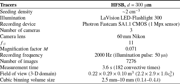
). Synchronisation of illumination and imaging systems is achieved through a LaVision programmable timing unit (PTU-X) controlled from a computer with the DaVis10 software. For each condition, a sequence of 7276 images is recorded at 2000 Hz (approximately 3.6 s measurement time). At this acquisition rate, a tracer in the free-stream region travels a distance of 2.5 mm (approximately 9 pixels) between subsequent frames. Details of the 3-D-PTV parameters are summarised in table 1.
Experimental parameters for 3-D-PIV measurements

Table 1 Long description
A table detailing experimental parameters for 3-D-PIV measurements. The table has 12 rows and 2 columns. Row 1: Tracers, HFSB, d = 300 μm. Row 2: Seeding density, ~2 cm^-3. Row 3: Illumination, LaVision LED-Flashlight 300. Row 4: Recording device, Photron Fastcam SA1.1 CMOS (1 Mpx sensor). Row 5: Number of cameras, 3. Row 6: Camera lens, 60 mm Nikon. Row 7: f#, 11. Row 8: Magnification factor M, 0.071. Row 9: Recording frequency, 2000 Hz (illumination pulse: 50 μs). Row 10: Number of images, 7276. Row 11: Measurement time, 3.6 s (182 convective times). Row 12: Field of view (3-D domain), 0.22 x 0.29 x 0.10 m^3 (2.2 x 2.9 x 1.0c0^3). Row 13: Cubic binning volume size, 2.5 mm–10 mm (0.1λ–0.4λ).
The image analysis is performed using the shake-the-box algorithm (Schanz et al. Reference Schanz, Gesemann and Schröder2016) in DaVis10. The raw images are preprocessed to remove the background caused by light reflections from the solid surface. Furthermore, the 3-D imaging system is calibrated to generate an image-to-space mapping function (Wieneke Reference Wieneke2008) and the optical transfer function (Schanz et al. Reference Schanz, Gesemann, Schröder, Wieneke and Novara2012). Residual disparity after self-calibration procedure is reduced to less than 0.1 pixels. At the given seeding concentration, approximately 6000 particles are detected in each recording, of which around 3500 particles are accepted into tracks. Figure 1(c) shows an example distribution of particle tracks in the measurement volume. The scattered velocity vectors are collected into a Cartesian grid of cubic bins. The binning procedure is performed at different levels of resolution, depending whether velocity vectors are accumulated to estimate statistics or for the instantaneous velocity field representation. For time-averaged results where particle tracks in the entire run are collected, smaller bin sizes of
 $0.1\lambda$
with 50 % overlap and
 $0.2\lambda$
with 75 % overlap are used for better spatial resolution, covering the measurement domain with a
 $173\times 225\times 71$
grid of vectors. A first-order spatial polynomial fits the data inside each bin, yielding unbiased velocity statistics at the bin centre (Agüera et al. Reference Agüera, Cafiero, Astarita and Discetti2016). To represent the time-varying velocity field, a larger bin size of
 $0.4\lambda$
is chosen, that encompasses 1 tracer particle per frame on average, and neighbouring bins overlap by 75 %. To increase the number of samples collected in each bin, data are accumulated from a relatively short time segment of 99 frames, corresponding to a normalised time interval of
 $\Delta t^* \equiv \Delta t U_{\infty }/c_0 = 2.5$
(here
 $^*$
denotes normalisation by the convective time scale
 $c_0/U_{\infty }$
). Also in this case the data are fitted in time with a first-order polynomial to reduce the effects of averaging.
The location and orientation of the aerofoil in the measurement volume are determined by reconstructing the 3-D locations of a pre-determined pattern of markers applied to the aerofoil. Marker detection is performed using an in-house MATLAB program (Li et al. Reference Li, Badia and Soare2024), which is based on the singular value decomposition solution to Wahba’s problem (Markley Reference Markley1988). The positional uncertainty of the markers is less than 0.2 mm, corresponding to less than
 $0.2^{\circ }$
for the angular position of the aerofoil.
2.3. Data assimilation using PINNs
The PINNs were employed to assimilate the scattered velocity field information, following the approach recently introduced by Steinfurth et al. (Reference Steinfurth, Cura, Fuchs, von Saldern, Oberleithner and Weiss2024 b). Compared with the binning procedure detailed in § 2.2, PINN assimilation eliminates the need for temporal averaging and yields pressure fluctuations that are consistent with the velocity fields governed by the Navier–Stokes equations.
Here, fully connected networks consisting of four hidden layers with 256 neurons map spatio-temporal coordinates
 $(x, y, z, t)$
to the corresponding velocity and pressure values
 $(u, v, w, p)$
. The networks were trained in a supervised fashion, constrained by the PTV data on the one hand and residuals of the governing equations on the other. The data and physics-informed losses were evaluated at all available PTV measurement points and 3000 randomly sampled collocation points per time step. Furthermore, a no-slip condition was embedded by penalising non-vanishing velocities for approximately 3000 points per time step evenly distributed across the aerofoil surface. Overall, this method allows us to anchor the model output with the available measurement data while constraining the solution space by the 3-D incompressible Navier–Stokes equations. A time series with a downsampled frequency of 100 Hz was obtained by constructing multiple PINN models – one for each time step. Each model was trained with a short measurement sequence (1 millisecond) by providing velocity data for the target time step as well as for one previous and one succeeding snapshot, which is necessary to determine temporal derivatives for the physics-informed loss term.
The PINN-based assimilation introduced by Steinfurth et al. (Reference Steinfurth, Hassanein, Doan and Scarano2024
b) was modified in the present study by adopting Fourier feature embeddings mapping the input layer to a higher-dimensional space using a sinusoidal transformation. The transformed input features higher-frequency components compared with the raw input data, which has been shown to address the bias towards learning (only) low-frequency components (Tancik et al. Reference Tancik, Srinivasan, Mildenhall, Fridovich-Keil, Raghavan, Singhal, Ramamoorthi, Barron and Ng2020). The mean absolute difference between PINN outputs and the PTV measurement data is below
 $0.1 U_\infty$
(supplementary movie S1).
2.4. Proper orthogonal decomposition
We perform POD on the 3-D velocity fluctuation field
 $\mathbf{u}(x,y,z,t)$
. The discretised
 $\mathbf{u}\equiv [u,v,w]$
is organised into a matrix
 $\mathsf{U}$
with dimensions of
 $N_s \times N_t$
, where
 $N_t$
is the number of time steps, and
 $N_s$
is the total number of spatial points. Note that all three velocity components are included in the POD input matrix
 $\mathsf{U}$
, and the velocity in regions without a valid measurement (such as inside or behind the aerofoil) is set to 0 so they do not contribute to the POD modes.
Following the singular value decomposition approach (Chatterjee Reference Chatterjee2000; Weiss Reference Weiss2019), the velocity matrix
 $\mathsf{U}$
can be expressed as
 \begin{equation} \mathsf{U} = \mathsf{\Phi }\mathsf{\Sigma }\mathsf{A}^T. \end{equation}
where superscript
 $T$
denotes matrix transpose,
 $\mathsf{\Phi } = [\phi _1,\phi _2,\ldots ,\phi _{N_s}]$
, with
 $\phi _k$
(
 $N_s\times 1$
column) representing the
 $k$
th mode basis and
 $\mathsf{A} = [a_1^T,a_2^T,\ldots ,a_{N_t}^T]$
, with
 $a_k$
(
 $1\times N_t$
row) representing the time coefficient of the
 $k$
th mode. Both
 $\mathsf{\Phi }$
and
 $\mathsf{A}$
are orthogonal matrices. Finally,
 $\mathsf{\Sigma }$
is a
 $N_s\times N_t$
diagonal matrix, and the diagonal elements consist of
 $\min (N_s,N_t)$
non-negative values arranged in descending order, i.e.
 $\lambda _1\geq \lambda _2\geq \cdots \geq \lambda _{\min (N_s,N_t)}\geq 0$
. Here,
 $\lambda _k^2$
represents the energy of the
 $k$
th mode.
The velocity fluctuations can then be reconstructed from the modes as
 \begin{equation} \mathbf{u_{\text{r}}}(x,y,z,t)=\sum _k{\lambda _k}a_k(t)\phi _k(x,y,z). \end{equation}
We use the PINN-assimilated velocity fluctuation data inferred on a Cartesian grid as input (see § 2.3), and perform POD using the MATLAB code of Zigunov (Reference Zigunov2019).
3. Velocity field statistics
3.1. Spanwise-periodic flow at small angle of attack
We first present the time-averaged flow at a small angle of attack of
 $\alpha = 5^{\circ }$
, where the flow pattern is spanwise-periodic with a wavelength of
 $\lambda$
. Figure 2(a-i)–(a-iii) shows the mean streamwise velocity
 $U$
in the peak, middle, and trough planes for case
 $A^*=0.1$
, and the straight-leading-edge baseline is included as figure 2(a-iv) for reference. The
 $A^*=0.05$
case shows a similar behaviour, therefore the velocity field is omitted here for conciseness. In all three planes,
 $U$
reaches its maximum around
 $x/c_0=0.3$
, but the velocity is higher in the trough plane compared with the peak plane, indicating a stronger suction. This observation is consistent with the potential flow theory prediction of van Nierop et al. (Reference van Nierop, Alben and Brenner2008), and the surface pressure measurements of Rostamzadeh et al. (Reference Rostamzadeh, Hansen, Kelso and Dally2014). Furthermore, in the trough plane (figure 2
a-iii) downstream of the suction peak, the stronger adverse pressure gradient promotes thickening of the boundary layer, leading to a significantly thicker low-speed region, which is visible when compared with the other planes of the tubercled aerofoil and the straight-leading-edge baseline aerofoil (figure 2
a-iv). The stronger suction peak in the trough plane (figure 2
a-iii) is caused by a larger effective angle of attack in the plane, which originates from an increased upwash produced by pairs of streamwise vortices formed around the edge of tubercles, as shown in figure 2(b). The vorticity is first concentrated close to the wall at
 $x/c_0 = 0.15$
, appearing as alternating strips with high
 $\omega _x$
. At approximately
 $x/c_0 = 0.3$
, the vortex cores become more circular as they undergo lift-up motion under their mutual induction. Further downstream at
 $x/c_0\geq 0.45$
, the size and strength of these vortices reduce, and the spanwise periodicity in the time-averaged vorticity field also reduces, which is attributed to the vortex interaction and weakening by the adverse pressure gradient. The increased unsteadiness of the flow is evidenced by the elevated turbulent kinetic energy
 $TKE\equiv \left (\overline {u^2}+\overline {v^2}+\overline {w^2}\right )/2$
behind tubercle troughs on the aft part of the aerofoil (see figure 2
c). At such a moderate incidence angle, the flow is highly modulated by the leading-edge tubercles and exhibits strong spanwise periodicity, and the flow pattern follows the same spatial phase as that of the leading-edge tubercles. Therefore, we can perform a spanwise phase average (denoted by
 $\widetilde {\omega }_x(x,y,z)$
) to show the 3-D flow field around the minimal repeating unit (i.e. one tubercle). Isosurfaces of streamwise vorticity are shown in figure 2(d), where the pair of counter-rotating streamwise vortices are clearly visible. As a result of wall blockage, the streamwise vortices tend to migrate away from the peak plane and approach their neighbours in the trough plane as they develop downstream. This behaviour is common to systems producing streamwise vortices of alternating rotation directions, such as in the vortex pair systems produced by conventional vane (Lögdberg et al. Reference Lögdberg, Fransson and Alfredsson2009) and micro-ramp vortex generators (Ye et al. Reference Ye, Schrijer and Scarano2016). At
 $x/c_0\gtrsim 0.3$
, the pair of streamwise vortices in the trough lift up from the surface, inducing secondary vortices of the opposite signs at the wall.
Time-averaged flow statistics of case
 $A^*=0.1$
at
 $\alpha =5^{\circ }$
. Streamwise velocity contours in (a-i) peak, (a-ii) middle and (a-iii) trough planes, and (a-iv) straight-leading-edge baseline. The baseline NACA0021 shape is marked by the black line. Contours of (b) time-averaged streamwise vorticity and (c) turbulent kinetic energy at
 $x/c_0=[0.15,\, 0.30,\, 0.45,\, 0.75,\, 1.20]$
. (d) Isosurface of spanwise ensemble-averaged vorticity at
 $\widetilde {\omega }_xc_0/U_{\infty }=[-0.4,\,0.4]$
(in blue and red, respectively).

Figure 2 Long description
Panel A: Four contour plots show streamwise velocity distributions at different planes: peak, middle, trough, and a straight-leading-edge baseline. The x-axis is labeled x/c0 and the y-axis is labeled z/c0. The contours are color-coded to represent different velocity ratios. Panel B: A 3D plot displays contours of time-averaged streamwise vorticity, with the color scale ranging from -5 to 5. Panel C: Another 3D plot shows contours of turbulent kinetic energy, with the color scale ranging from 0 to 0.02. Panel D: An isosurface plot illustrates spanwise ensemble-averaged vorticity, highlighting secondary vortices and a streamwise vortex pair.
3.2. Spanwise modulation by stall cells
3.2.1. Time-averaged velocity fields of steady stall-cell patterns
Post-stall flow fields. (a-i)-(a-iii) Streamwise velocity contours of case
 $A^*=0.1$
at
 $\alpha = 15^{\circ }$
in the trough planes marked by
 $\unicode {x2460}$
–
 $\unicode {x2462}$
in (b-i), and (a-iv) straight-leading-edge baseline. Regions of steady flow separation, shown by isosurfaces of
 $U/U_{\infty } = -0.01$
and surface streamlines, case
 $A^*=0.1$
at (b-i)
 $\alpha =15^{\circ }$
, (b-ii)
 $\alpha =20^{\circ }$
and (b-iii)
 $\alpha =25^{\circ }$
; case
 $A^*=0.05$
at (c-i)
 $\alpha =15^{\circ }$
and (c-ii)
 $\alpha =20^{\circ }$
. (d) Ratio between the separated and total area of the aerofoil upper surface,
 $r_{\mathrm{sep}}$
, for near- and post-stall angles. Symbols represent the time-averaged
 $r_{\mathrm{sep}}$
at each
 $\alpha$
, and error bars are the upper and lower bounds of the instantaneous fluctuations.

The flow exhibits a steady separation pattern for
 $\alpha$
values between 15
 $^{\circ }$
and 25
 $^{\circ }$
for case
 $A^*=0.1$
, and the
 $\alpha$
range narrows to between 15
 $^{\circ }$
and 20
 $^{\circ }$
for case
 $A^*=0.05$
. Time-averaged flow patterns of these cases are shown in figures 3(b) and 3(c), where the separated regions are depicted by the green isosurfaces of zero mean streamwise velocity. Following the extended Runge–Kutta method detailed by Wu et al. (Reference Wu, Cao and Dong2022), streamlines are first calculated in three dimensions and then projected on a surface offset by 4 mm from the aerofoil to avoid vanishing velocity and spurious data in close proximity to the solid wall.
Stall cells with a width of
 $\mathcal{O}(c_0)$
appear in all cases in figures 3(b) and 3(c), with their centrelines at tubercle troughs. Flow separation extends across the entire chord, from the tubercle trough to the trailing edge. In contrast, for straight-leading-edge aerofoils, separation typically initiates at a portion of the chord away from the leading edge (Manolesos & Voutsinas Reference Manolesos and Voutsinas2014), but stall-cell inception from near the leading edge has been observed at lower Reynolds numbers of
 $Re_c\simeq 1.5\times 10^5$
(Khaleghizadeh et al. Reference Khaleghizadeh, Scarano and Li2024). The widths of the separated regions of case
 $A^*=0.1$
are smaller than those of
 $A^*=0.05$
at the same
 $\alpha$
, indicating that the tubercles with larger amplitudes are more effective in compartmentalising the separated regions. For each tubercle geometry, the stall cell also widens with increasing
 $\alpha$
: for the narrow stall cell of case
 $A^*=0.1$
at
 $\alpha = 15^{\circ }$
(figure 3
b-i), the spacing between the two foci is approximately
 $2\lambda$
(equivalently
 $0.5c_0$
) and the width of the entire structure based on surface streamlines is around
 $c_0$
, which is smaller than that of the typical stall cells formed on aerofoils with a straight leading edge (Yon & Katz Reference Yon and Katz1998). When
 $\alpha$
is further increased to
 $25^{\circ }$
(figure 3
b-iii), a wide stall cell emerges. The structure remains steady, but the spacing between two foci has increased to roughly
 $6\lambda$
(or
 $1.5c_0$
). The width of the entire cell becomes around
 $2c_0$
, similar to that of stall cells formed on aerofoils with a straight leading edge (Yon & Katz Reference Yon and Katz1998). In addition to the stall cell, small separation bubbles appear in the tubercle troughs in between, generated by the localised upwash from the counter-rotating streamwise vortices. The size of these bubbles increases with increasing distance from the large stall cells.
Figure 3(a-i)–(a-iv) compares the detailed flow field of a stall cell in several
 $xz\hbox{-}$
slices with the straight-leading-edge baseline at the same incidence angle of
 $\alpha = 15^{\circ }$
. Note that the mean flow field in the baseline case is homogeneous along the span, so only one
 $xz\hbox{-}$
slice is shown here for conciseness. In the stall-cell centreplane (slice
 $\unicode {x2460}$
, figure 3
a-i), the shear layer is much higher compared with that in the baseline case (figure 3
a-iv). As the distance from the stall cell increases, a smaller separation bubble appears in the trough at slice
 $\unicode {x2462}$
, while the aerofoil section continues to generate substantial lift, as evidenced by the high-speed region above the separation bubble (figures 3
a-ii and 3
a-iii). The effect of sidewalls and associated junction flows on these observations is expected to be minimal. The boundary layer thickness on the sidewalls at the aerofoil location is estimated to be less than 3 cm, or
 $0.3c_0$
. Previous works on the formation of stall cells (Gregory et al. Reference Gregory, Quincey, O’Reilly and Hall1971) demonstrate that sidewall boundary layer and junction flow make little difference to the formation of stall cells. In addition, the tubercles generate a system of streamwise vortices with strong spanwise components, therefore, it is expected that they further prohibit the influence from the junction flow on the stall cells. Furthermore, the measurement domain only covers the middle
 $2.9c_0$
of the full
 $6c_0$
span of the test section. In summary, we do not expect to see any substantial sidewall effect in the measured velocity fields.
The stall cells are arranged along the span without a specific periodicity. The distance
 $S$
between two neighbouring stall-cell centrelines for all cases and incidence angles is summarised in table 2, in comparison with the Reynolds-averaged Navier–Stokes simulation results of a configuration similar to
 $A^*=0.05$
by Cai et al. (Reference Cai, Zuo, Maeda, Kamada, Li, Shimamoto and Liu2017). At
 $\alpha = 15^{\circ }$
,
 $A^*=0.05$
and Cai et al. (Reference Cai, Zuo, Maeda, Kamada, Li, Shimamoto and Liu2017) have similar stall-cell spacings. However, at
 $\alpha = 25^{\circ }$
, no stable stall cell is found in the
 $A^*=0.05$
case, whereas Cai et al. (Reference Cai, Zuo, Maeda, Kamada, Li, Shimamoto and Liu2017) observed stable stall cell with a slightly higher spacing (
 $S/\lambda =7$
). This difference in the separated flow pattern can be attributed to the difference in the Reynolds number, or baseline aerofoil geometry.
Spacing between centrelines of stall cell (
 $S/\lambda$
) at various
 $\alpha$

Table 2 Long description
A table comparing spacing between centrelines of stall cells at various angles. The table has 4 rows and 4 columns. The columns are labeled with different angles (alpha = 15°, alpha = 20°, alpha = 25°) and a reference (Cai et al. (2017)). The row labels are A* = 0.05, A* = 0.1, and Cai et al. (2017). Row 1: A* = 0.05, alpha = 15°, 6; alpha = 20°, 6; alpha = 25°, unsteady; Cai et al. (2017), 6. Row 2: A* = 0.1, alpha = 15°, 4, 7; alpha = 20°, 3, 4; alpha = 25°, 9; Cai et al. (2017), 7. Row 3: Cai et al. (2017), alpha = 15°, 5, 6; alpha = 20°, -; alpha = 25°, 7.
3.2.2. Instantaneous flow separation
The degree of instantaneous flow separation can be quantified through
 $r_{\mathrm{sep}}$
, the ratio between the separated and total area of the aerofoil upper surface in the measurement volume. The values of this ratio are summarised in figure 3(d), and some example videos are included as supplementary movies S2–6. At
 $\alpha =0^{\circ }$
and
 $5^{\circ }$
, all three aerofoils exhibit fully attached flow (
 $r_{\mathrm{sep}} = 0$
). Note that laminar separation bubbles are a common feature for aerofoils in a similar low-Reynolds-number regime (O’Meara & Mueller Reference O’Meara and Mueller1987), and have also been previously observed on tubercled aerofoils (Sudhakar et al. Reference Sudhakar, Karthikeyan and Suriyanarayanan2019). However, laminar separation bubbles typically have a very small height of
 $\lesssim 0.02c_0$
, which is beyond the limit of the spatial resolution in the present measurements with a binning volume size of
 $0.2\lambda$
(equivalently
 $0.05c_0$
) and the lower data density approaching the solid surface. Nevertheless, the main purpose of calculating
 $r_{\mathrm{sep}}$
is to study the evolution of the large-scale separations, whereas resolving laminar separation bubbles is beyond the scope of the current work. At
 $\alpha =10^{\circ }$
, the flow remains fully attached for the baseline aerofoil, but stall cells appear intermittently on the tubercled aerofoils (see supplementary movie S3). For
 $\alpha \geq 15^{\circ }$
, the baseline flow is almost fully separated from the leading edge, while the separated area gradually increases with
 $\alpha$
for the tubercled aerofoils. The separated area on
 $A^*=0.1$
case is consistently lower than that on
 $A^*=0.05$
.
The evolution of separated area with
 $\alpha$
provides a possible explanation for the effect of tubercles on aerodynamic forces (Johari et al. Reference Johari, Henoch, Custodio and Levshin2007; Hansen et al. Reference Hansen, Kelso and Dally2011; Cai et al. Reference Cai, Zuo, Maeda, Kamada, Li, Shimamoto and Liu2017). At small
 $\alpha$
, the flow remains fully attached regardless of the presence of tubercles. In the linear-lift regime, the contribution of induced upwash and downwash to the overall lift cancels out across the span, therefore the change in lift and drag forces is negligible. Immediately prior to the stall angle, the upwash generated at the tubercle troughs triggers an early large-scale flow separation, which could be unsteady and intermittent in nature. This leads to a reduction in lift and an increase in drag. In contrast, the flow on the baseline aerofoil remains fully attached, producing higher lift and lower drag. When
 $\alpha$
exceeds the stall angle, the flow separates from the baseline aerofoil more coherently across the entire span, resulting in a sudden and global loss of lift (increase in drag). In contrast, the tubercled aerofoil copes with the higher incidence by forming separated cells, which in turn induces a downwash motion at their boundaries, keeping the flow attached. One may conclude that by sacrificing part of the lift-generating surface, the overall lift generation is retained on the remaining part of the aerofoil surface, resulting in an overall more gradual and gentle stall behaviour. This observation confirms the compartmentalisation mechanism of tubercles reported by Cai et al. (Reference Cai, Zuo, Maeda, Kamada, Li, Shimamoto and Liu2017, Reference Cai, Zuo, Morimoto, Maeda, Kamada and Liu2018).
4. Pressure estimation from velocity fields
To relate the flow field observation to the aerodynamic performance of the aerofoil, the surface pressure is evaluated from the measured velocity field. Following van Oudheusden (Reference van Oudheusden2013), the time-averaged static pressure gradient
 $\nabla \overline {p}$
can be expressed as
 \begin{equation} \nabla \overline {p} = -\rho \left (\mathbf{U}\cdot \nabla \right )\mathbf{U}-\rho \nabla \cdot \overline {\boldsymbol{uu}}, \end{equation}
where
 $\mathbf{U}\equiv [U, V, W]$
and
 $\mathbf{u}\equiv [u,v,w]$
represent the time-averaged velocity components and fluctuations, respectively. The viscous term is commonly excluded from the computation because its contribution is negligible at high Reynolds numbers (
 $Re\gt 10^3$
), as previously demonstrated (van Oudheusden et al. Reference van Oudheusden, Scarano, Roosenboom, Casimiri and Souverein2007; Ghaemi et al. Reference Ghaemi, Ragni and Scarano2012). The time-averaged velocity and Reynolds stress terms are derived from the binned PTV data, and their gradient is estimated using a central difference scheme.
The 3-D spatial marching pressure integration algorithm developed by Jux et al. (Reference Jux, Sciacchitano and Scarano2020) is used here. The computational domain is divided into two regions: in the irrotational region, the static pressure is obtained following the Bernoulli relation; in the turbulent wake and close to the object, the pressure gradient in (4) is integrated. This approach reduces the error propagation produced during the spatial marching by minimising the region where the equation (4) is numerically evaluated. The domain partitioning is obtained by identifying the rotational region on the basis of the local turbulence intensity
 $\left (\left (\overline {u^2}+\overline {v^2}+\overline {w^2}\right )/3\right )^{1/2}/U_{\infty }$
. A minimum threshold of
 $5\%$
is conservatively chosen for robustness, and the identified rotational region is then dilated by a filter with a diameter of
 $5$
mm to eliminate contamination in the irrotational region Jux et al. (Reference Jux, Sciacchitano and Scarano2020). The pressure distribution approaching the aerofoil surface is then computed by integrating (4) from the nearest fluid mesh node to the surface node. For further details, readers are referred to the work of Jux et al. (Reference Jux, Sciacchitano and Scarano2020).
Top view of mean static pressure coefficient of case
 $A^*=0.1$
at (a-i)
 $\alpha = 5^{\circ }$
and (a-ii)
 $\alpha = 15^{\circ }$
; straight-leading-edge baseline at (b-i)
 $\alpha = 5^{\circ }$
and (b-ii)
 $\alpha = 15^{\circ }$
. Standard deviation of the PINN-assimilated pressure coefficient for (c-i) case
 $A^*=0.1$
and (c-ii) baseline at
 $\alpha = 15^{\circ }$
. (d) Connected symbols: lift coefficient
 $C_{L}$
for
 $A^* = [0, 0.05, 0.1]$
at
 $\alpha = 0^{\circ }$
–
 $30^{\circ }$
, with the pressure-side contribution estimated from XFOIL simulations (dashed line, Ncrit = 7, where Ncrit is the log of the amplification factor of the most-amplified frequency which triggers transition). The dot-dashed lines are load cell data from Johari et al. (Reference Johari, Henoch, Custodio and Levshin2007) at
 $Re = 1.83\times 10^5$
, and the black, orange and green colours correspond to the same tubercle geometries as in the present work.

The time-averaged surface pressure distributions for the
 $A^*=0.1$
and 0 cases at selected
 $\alpha$
values are shown in figures 4(a) and 4(b). The pressure coefficient is defined as
 $\overline {C_p}\equiv \frac {\overline {p}-p_{\infty }}{\frac {1}{2}\rho U_{\infty }^2}$
, where
 $p_{\infty }$
is the far-field static pressure. At
 $\alpha = 5^{\circ }$
, the flow remains attached in both cases, with the accelerated flow above the aerofoil creating a suction peak (dark blue regions in the figure) near the leading edge. The negative
 $\overline {C_p}$
gradually recovers downstream. The tubercled aerofoil (figure 4
a-i) features spanwise modulation with weaker suction behind the peaks and stronger suction behind the troughs. This behaviour aligns with the fact that tubercles generate downwash behind the peaks and upwash behind the troughs, leading to decreased and increased effective angles of attack, respectively, as discussed in § 3.1 and depicted in figure 2(a). When
 $\alpha$
is increased to
 $15^{\circ }$
, the flow becomes fully separated in the baseline case, and the suction peak vanishes entirely (as evidenced by the absence of dark blue regions in figure 4
b-ii). In contrast, for the
 $A^*=0.1$
case, a strong suction region can still be observed in regions of flow streaming between stall cells. The unsteadiness of the surface pressure is quantified by
 ${\overline {C_p^2}}^{1/2}$
, the standard deviation of instantaneous surface pressure coefficients assimilated by PINN. The tubercled case (figure 4
c-i) exhibits a higher standard deviation compared with the baseline (figure 4
c-ii), especially in the attached flow region where the magnitude of
 $\overline {C_p}$
is the highest.
The aerodynamic force and its decomposition into lift and drag cannot be obtained from the suction-side analysis solely. However, the contribution from the pressure side is expected to exhibit less variation with
 $\alpha$
and between different cases. Therefore, the lift coefficient can be computed from the surface pressure data following
 \begin{equation} C_{L} = -\frac {1}{bc_0}\iint \overline {C_p}\cos \theta \mathrm{d}A+C_{L,\text{p}}, \end{equation}
where
 $b$
is the span of the integrated area (approximately
 $2.25c_0$
),
 $\mathrm{d}A$
is the area of the surface element,
 $\theta$
is the angle between the surface element normal vector and the
 $z\hbox{-}$
direction and
 $C_{L,\text{p}}$
is the contribution from the pressure side estimated using the XFOIL simulation of a 2-D aerofoil section at the same Reynolds number. The lift coefficient results are summarised in figure 4(d), in comparison with the load cell data of Johari et al. (Reference Johari, Henoch, Custodio and Levshin2007) from the same tubercle geometries at a higher Reynolds number,
 $Re = 1.83\times 10^5$
. The current baseline aerofoil reaches the maximum
 $C_{L}=0.84$
at
 $\alpha = 10^{\circ }$
, followed by a sudden reduction to 0.47 at
 $\alpha = 15^{\circ }$
. The continuing increase of
 $C_{L}$
post-stall up to (and potentially beyond)
 $\alpha =30^{\circ }$
is also consistent with the literature (Rogowski et al. Reference Rogowski, Mikkelsen, Michna and Wiśniewski2025). The sudden loss of lift of the baseline model at
 $\alpha = 10^{\circ }$
corresponds to the sharp onset of flow separation, which is homogeneous along the aerofoil span (see figure 3
d for comparison). In contrast,
 $C_{L}$
remains steady for
 $\alpha \gt 10^{\circ }$
in both
 $A^*=0.05$
and 0.1 cases, which is a result of the combined effect of increasing
 $\alpha$
modifying the overall pressure distribution, and the gradual increase in the separated area in figure 3(d). The lift coefficient behaviour and trends with increasing tubercle amplitude are qualitatively similar to the results of Johari et al. (Reference Johari, Henoch, Custodio and Levshin2007) at
 $Re = 1.83\times 10^5$
, despite a shift in the stall angle and maximum lift coefficient. In summary, these results demonstrate that leading-edge tubercles still exhibit a stall-softening effect at a lower Reynolds number of
 $Re=3.3\times 10^4$
.
5. Modal analysis of stall cell
5.1. Single stall cell
(a) Energy distribution in the first 30 POD modes of the stall cell at
 $y/c_0 = -0.25$
,
 $A^*=0.1$
,
 $\alpha = 15^{\circ }$
. Left axis: energy fraction of each mode; right axis: cumulative sum of the energy fraction. (b) Pre-multiplied energy spectrum of the time coefficient
 $a_k(t)$
. The dotted blue line is the energy spectrum of the PINN-assimilated pressure signal at a point in the stall cell
 $(x/c_0,y/c_0, z/c_0) = (0.9,-0.3,0.05)$
. (c) Shapes of the first three POD modes, case
 $A^*=0.1$
,
 $\alpha = 15^{\circ }$
. Red and blue isosurfaces are at
 $u_k=0.004$
and
 $-0.004$
, respectively. Green isosurfaces are at
 $U/U_{\infty } = 0$
, illustrating time-averaged separated flow region. The POD is performed in the region bounded by the black lines.

Figure 5 Long description
Panel A: A bar and line graph show the energy distribution in the first 30 POD modes of the stall cell. The left vertical axis represents the energy fraction of each mode, while the right vertical axis shows the cumulative sum of the energy fraction. The horizontal axis is labeled with the mode index k. The bar graph indicates the energy fraction for each mode, and the line graph shows the cumulative energy fraction. Panel B: A line graph displays the pre-multiplied energy spectrum of the time coefficient. The horizontal axis is labeled St, and the vertical axis is labeled with a normalized energy spectrum. The graph includes multiple lines representing different modes and a dotted blue line for the energy spectrum of the PINN-assimilated pressure signal. Panel C: Three 3D visualizations show the shapes of the first three POD modes. Each visualization includes red and blue isosurfaces at specific values and green isosurfaces illustrating the time-averaged separated flow region. The visualizations are bounded by black lines.
We first perform a modal analysis on a single stall cell, which is observed on
 $A^*=0.1$
at
 $\alpha = 15^{\circ }$
. To isolate the dynamics of a single stall cell, and reduce the influence of noise in the data, we select a spanwise length of
 $4\lambda$
centred about the stall cell, and remove any data points with poor optical access (within or behind the aerofoil), in the vicinity (less than 4 mm) of the surface, or above the tubercles. The volume of data used as input to POD is visualised by the black lines in figure 5(c).
The energy distribution of the first 30 POD modes is shown in figure 5(a). The first mode contributes to nearly 24 % of the total turbulent kinetic energy, and the energy fraction quickly diminishes at higher modes. Isosurfaces of the
 $u$
-component in the first three modes are shown in figure 5(c). The extent of the separation captured by the first mode can be illustrated through the
 $(U+u_{\mathrm{r}})/U_{\infty }=0$
contour lines at the maximum (red) and minimum (blue) values of the time coefficient
 $a_1(t)$
(figure 6
a-i and figure 6
c-i), where
 $u_{\mathrm{r}}$
is the velocity fluctuation reconstructed by (3) using the first mode only. The separation point appears to be time-independent, therefore the motion is consistent with the flapping (Thacker et al. Reference Thacker, Aubrun, Leroy and Devinant2013; Schrijer et al. Reference Schrijer, Sciacchitano and Scarano2014), rather than breathing (Mohammed-Taifour & Weiss Reference Mohammed-Taifour and Weiss2016), motion of a separation bubble, which features a low-frequency up-and-down movement of the shear layer.
A negative
 $a_1$
is associated with an expansion of the separated region, and the largest separation bubble is almost twice the thickness of the smallest (positive
 $a_1$
), confirming that the flapping motion is a dominant mode of the separation bubble dynamics.
Contour plots of POD modes, case
 $A^*=0.1$
at
 $\alpha = 15^{\circ }$
. Panels (a-i) and (a-ii) show the
 $u$
-component, and (b-i) and (b-ii) show the
 $w$
-component of the first two modes in the
 $xz$
-plane at
 $y/c_0=-0.25$
(centreplane of the stall cell). Red and blue dots denote positive and negative peaks, respectively, in
 $u_2$
and
 $w_2$
, and the streamwise distance between the pair corresponds to
 $\lambda _c/2$
. Panels (c-i)-(c-iii) present the
 $u$
-component of the first three modes in the
 $yz$
-plane at
 $x/c_0=0.9$
. In all plots, the thick black contour line indicates
 $U/U_{\infty }=0$
from the time-averaged flow field, while the red dashed line and blue dot-dashed line mark the extent of the separation bubble at the maximum and minimum of
 $a_k(t)$
, respectively.

The mode’s temporal frequencies are further investigated using pre-multiplied energy spectra of the time coefficients, as summarised in figure 5(b). The Strouhal number is defined as
 $St\equiv fc_0/U_{\infty }$
, which is the frequency normalised by the free-stream velocity and mean chord length. The dominant frequency of the first mode is at a Strouhal number of
 $St=0.16$
, and the peak is also found in the spectrum of pressure.
The second spatial mode features a reduction in the streamwise wavelength, as evidenced by the isosurface in figure 5(c-ii), and the velocity contours in figures 6(a-ii) and 6(b-ii). Here, a negative
 $a_2$
leads to a dented front part and a thicker aft body of the separation bubble in the centreplane, corresponding to an sweep (
 $u\gt 0$
and
 $w\lt 0$
) at the front and a ejection (
 $u\lt 0$
and
 $w\gt 0$
) at the back. The characteristics of the first two modes are very similar to previous reports on a single separation bubble utilising planar PIV (Schrijer et al. Reference Schrijer, Sciacchitano and Scarano2014; Mohammed-Taifour & Weiss Reference Mohammed-Taifour and Weiss2016). In those studies, the second and third modes were identified as a convective pair, and the distance between the positive and negative peaks in the modal velocity is the half-wavelength
 $\lambda _c/2$
. We attempt to measure the
 $\lambda _c/2$
in the second mode only, and assuming a convective velocity of
 $0.67U_{\infty }$
(Thacker et al. Reference Thacker, Aubrun, Leroy and Devinant2013), the frequency is estimated to be
 $f_2\equiv U_c/\lambda _c=22.3$
Hz, which is equivalent to a Strouhal number of
 $St = 0.45$
, close to the broad second peak found around
 $St = 0.38$
in the pre-multiplied energy spectrum (figure 5
b).
The Strouhal numbers of the first two modes can be compared with previous works in the literature. Note that our definition of the Strouhal number uses a length scale of
 $c_0$
, which is representative of the separation bubble length. Strouhal numbers of other studies will be converted to the definition with separation bubble length or aerofoil chord length. The Strouhal number of the flapping motion is approximately 0.16 in the current data, which is within the range of 0.15 to 0.21 observed in the surface pressure signal of stall cells on a straight-leading-edged aerofoil by Yon & Katz (Reference Yon and Katz1998). This is also similar to the values reported by Schrijer et al. (Reference Schrijer, Sciacchitano and Scarano2014) (
 $St = 0.10{-}0.14$
) and Thacker et al. (Reference Thacker, Aubrun, Leroy and Devinant2013) (
 $St = 0.11$
) for the shear-layer flapping motions in geometry-induced separations, but higher than the value of
 $St\simeq 0.01$
found by Mohammed-Taifour & Weiss (Reference Mohammed-Taifour and Weiss2016) of the ‘breathing’ motion (contraction/expansion of the whole bubble) of a pressure-gradient-induced turbulent separation bubble. The frequency of the second mode compares favourably with the values of Mohammed-Taifour & Weiss (Reference Mohammed-Taifour and Weiss2016) (
 $St = 0.35$
), Schrijer et al. (Reference Schrijer, Sciacchitano and Scarano2014) (
 $St = 0.4$
) and Thacker et al. (Reference Thacker, Aubrun, Leroy and Devinant2013) (
 $St = 0.6{-}0.7$
). The flapping and shedding behaviours are also presented in the time-series animation of the velocity field reconstructed from the first three POD modes (supplementary movie S7). This suggests that the stall cell formed on a tubercled aerofoil behaves similarly as turbulent separation bubbles.
In the present work, the third mode (figure 5
c-iii) obtained from volumetric data captures the spanwise anti-symmetry of the separation bubble. This is similar to the second mode observed by Steinfurth et al. (Reference Steinfurth, Cura, Fuchs, von Saldern, Oberleithner and Weiss2024
a) in the velocity field in the
 $yz$
-plane of a turbulent separation bubble on a one-sided diffuser. This mode captures the expansion of the separation bubble on one side of the centreplane, accompanied by the contraction on the other side. A closer examination of figure 5(c-iii) and figure 6(c-iii) reveals that the shape of the third mode is not entirely mirror symmetrical. Stronger modal velocity and larger variation in the
 $U=0$
contour line in the
 $yz$
-plane are shown on the negative
 $y$
side of the stall cell, which is
 $4\lambda$
away from the neighbouring stall cell. In contrast, the positive
 $y$
side experiences less unsteadiness in this mode. One possible reason is that some of the fluctuations are captured by other modes (e.g. mode 2, figure 5
c-ii, and higher-order modes). In addition, the flow field surrounding the stall cell is not symmetrical: the distance between the centreline of the stall cell in the boxed region and its nearest neighbour is only
 $4\lambda$
on the left, but reaches
 $7\lambda$
on the right. More controlled datasets on isolated or neighbouring stall cells are required in future works to decipher the interaction between neighbouring stall cells and its effect of the axisymmetry of the modes.
(a) Energy distribution in the first 30 POD modes of the stall cell at
 $y/c_0 = -0.25$
,
 $A^*=0.1$
,
 $\alpha = 20^{\circ }$
. Left axis: energy fraction of each mode; right axis: cumulative sum of the energy fraction. (b) Pre-multiplied energy spectrum of the time coefficient
 $a_k(t)$
. (c) Shapes of the first three POD modes,
 $A^*=0.1$
,
 $\alpha = 15^{\circ }$
. Red and blue isosurfaces are at
 $u_k=0.004$
and
 $-0.004$
, respectively. Green isosurfaces are at
 $U/U_{\infty } = 0$
, illustrating time-averaged separated flow region. The POD is performed in the region bounded by the black lines.

5.2. Neighbouring stall cells
The interaction between two neighbouring stall cells is studied in this section, using the data acquired at
 $\alpha = 20^{\circ }$
for the case
 $A^*=0.1$
. The interaction between the two neighbouring cells (‘jostling’) was observed qualitatively using tufts on a straight-leading-edged aerofoil (Yon & Katz Reference Yon and Katz1998), and here we aim to provide a quantitative assessment of the interaction based on the POD modes. The POD is performed on a domain of
 $-0.75\lt y/c_0\lt 1.25$
, which encapsulates two stall cells with the centrelines at
 $y/c_0=-0.25$
and 0.75.
The energy distribution of the POD modes is summarised in figure 7(a), and the shapes of the first three modes are shown in figure 7(c) (see also supplementary movie S8). The first mode features
 $180^{\circ }$
out of phase expansion/contraction of the two stall cells, which contains approximately 11 % of the total energy. In contrast, the second mode captures simultaneous expansion/contraction and contains 9.6 % of the total energy. The higher energy in the first mode indicates a stronger tendency for the two stall cells to be
 $180^{\circ }$
out of phase, i.e. when one stall cell expands, the neighbouring stall cell tends to shrink in size. The sum of the energy in these first two modes is approximately 21 %, similar to the energy fraction of the flapping mode of a single stall cell (the first mode in figure 5
c-i), suggesting that the energy of the flapping motion of two neighbouring stall cell is distributed in the first two modes (simultaneous or out of phase). The third mode (figure 7
c-iii) is a combination of the streamwise shedding and spanwise anti-symmetric modes. Higher-order modes contain smaller-scale structures with less apparent symmetry features.
The pre-multiplied energy spectrum of the first and second modes peaks at
 $St=0.125$
(figure 7
b), similar to that of the single stall cell (figure 5
b). The magnitude of the low-frequency peak reduces in higher-order modes, and the energy increases in the higher-frequency range of
 $St\approx 0.3$
, in agreement with the previously observed shedding frequency.
5.3. Spanwise modes in the absence of stable stall cells
As previously discussed, case
 $A^*=0.1$
at
 $\alpha = 30^{\circ }$
exhibits no stable stall cells. The POD modes of this cases are summarised in figure 8(c). In each POD mode, there are tubercle wavelength
 $\lambda$
-scaled structures, as well as larger structures that span two or more
 $\lambda$
with alternating signs. The time coefficients and their pre-multiplied energy spectra are shown in figures 8(a) and 8(b), respectively. There are considerable amounts of energy contained in very low frequencies of
 $St\lt 0.008$
that remain unresolved in the present work, as limited by the length of the time series and window size for calculating the energy spectrum.
These POD modes do not represent a single stall cell, instead, their temporal modulation by the time coefficients captures the emergence of separation patches by merging separation bubbles from the neighbouring tubercle troughs. These modes reveal the dynamics and organisation of the separated flow on a tubercled aerofoil in the deep-stall regime, which is substantially different from that of a straight-leading-edge baseline.
(a) Time coefficients of the first three modes and (b) their pre-multiplied energy spectrum,
 $A^*=0.1$
,
 $\alpha = 30^{\circ }$
; (c-i)-(c-iii) are the first three POD modes. Red and blue isosurfaces are at
 $u_k=0.004$
and
 $-0.004$
, respectively. Green isosurfaces are at
 $U/U_{\infty } = 0$
, illustrating time-averaged separated flow region. POD is performed in the region bounded by the black lines.

Figure 8 Long description
Panel A: A line graph shows the time coefficients of the first three modes. The x-axis is labeled 'tU∞/c_0' and the y-axis is labeled 'a_(t)'. Three lines represent Mode 1, Mode 2, and Mode 3, each with different colors. Panel B: Another line graph displays the pre-multiplied energy spectrum of the first three modes. The x-axis is labeled 'St' and the y-axis is labeled 'fϕ_kk;/āk²'. Three lines represent Mode 1, Mode 2, and Mode 3, each with different colors. Panels C-i, C-ii, and C-iii: Three 3D visualizations show the first three POD modes. Red and blue isosurfaces are at specific levels, and green isosurfaces illustrate the time-averaged separated flow region. The visualizations are bounded by black lines.
6. Concluding remarks
The present study has examined the phenomenon of spanwise modulation of the flow over full-span aerofoils with a tubercled leading edge, both in the attached and separated flow regime. The use of high-speed 3-D-PTV enables us to analyse the velocity vector and its gradient in a volumetric domain, and to further examine the flow properties in close proximity of the aerofoil surface. The unsteady 3-D behaviour of the separated flow is captured, and analysed both qualitatively and quantitatively with the aid of PINN data assimilation and POD. The time-average surface pressure distribution is also obtained with a data reduction that invokes the Reynolds-averaged Navier–Stokes equations. The main findings are summarised as follows.
At a small angle of
 $\alpha = 5^{\circ }$
, the flow exhibits spanwise periodicity, with pairs of streamwise vortices emanating from the tubercles. Comparing the flow fields in the trough and the peak planes, the former has a thicker boundary layer, and a higher effective angle of attack as a result of the upwash induced by these streamwise vortices. With
 $\alpha$
increasing to
 $15^{\circ }-20^{\circ }$
, stable stall cells appear at a fixed trough throughout each observation, with a width of approximately
 $4\lambda$
or
 $c_0$
. The time-resolved data also reveal two types of unsteadiness of the stall cells: at
 $\alpha = 10^{\circ }$
, isolated stall cells appear and disappear intermittently with a lifespan of
 $\mathcal{O}(50c_0/U_{\infty })$
. At
 $\alpha \gtrsim 25^{\circ }$
, the stall cells become once again mobile along the span, as a result of competitive growth between separated regions originating from different troughs.
Using the pressure from PIV and PINN assimilation, we provide direct evidence supporting the compartmentalisation mechanism and its effect on stall softening: as
 $\alpha$
exceeds the stall angle, isolated stall cells form on the tubercled aerofoils, outside of which the flow remains attached and continues to generate high lift, whereas the baseline aerofoil exhibits a full-span separation. However, the higher lift generated by a tubercled aerofoil at intermediate angles is accompanied by stronger fluctuations in the pressure distribution.
Finally, POD analysis reveals that stable stall cells formed on tubercled aerofoils post-stall (
 $15^{\circ }\lesssim \alpha \lesssim 20^{\circ }$
) share characteristics with turbulent separation bubbles: the first three POD modes capture its flapping motions, streamwise shedding and spanwise anti-symmetry. The flapping motion has a low frequency of
 $St\sim \mathcal{O}(0.1)$
, and the streamwise shedding motion has a frequency of
 $St\sim \mathcal{O}(0.4)$
. The flapping motions of neighbouring stall cells tend to be
 $180^{\circ }$
out of phase. In the deep-stall regime (
 $\alpha = 30^{\circ }$
), no stable stall cell forms, and the POD analysis captures the long-term (
 $\mathcal{O}(50c_0/U_{\infty })$
) dynamics of the emergence and interaction of separation bubbles.
In summary, this study provides a unified picture of how the flow field induced by leading-edge tubercles evolves from the attached to the separated regime, and more importantly, the unsteadiness of the stall cells. By combining surface pressure measurements with volumetric velocity fields, we confirm that the ability of tubercles to soften stall arises from the controlled, spatially localised growth of separated regions. Moreover, we reveal that stall cells share modal characteristics with turbulent separation bubbles. From an application standpoint, these results imply an inherent trade-off introduced by tubercles: while separation compartmentalisation mitigates abrupt stall, it is accompanied by the unsteadiness associated with the stall-cell dynamics in the post-stall regime.
Supplementary material
Supplementary information is available at https://doi.org/10.1017/flo.2026.10068.
Acknowledgements
The authors gratefully acknowledge the technical support of Mr F.J. Donker Duyvis and the assistance of Mr P. Valls Badia in experimental data acquisition.
Data availability statement
Velocity field data are available from the corresponding author (M.L.).
Funding statement
This research received no specific grant from any funding agency, commercial or not-for-profit sectors.
Competing interests
The authors declare no conflicts of interest.
Ethical standards
The research meets all ethical guidelines, including adherence to the legal requirements of the study country.


 λ
 A
 A∗=0.1
 α=0∘
 A∗=0.1
 α=15∘

 A∗=0.1
 α=5∘
 x/c0=[0.15,0.30,0.45,0.75,1.20]
 ω~xc0/U∞=[−0.4,0.4]

 A∗=0.1
 α=15∘
 ①
 ③
 U/U∞=−0.01
 A∗=0.1
 α=15∘
 α=20∘
 α=25∘
 A∗=0.05
 α=15∘
 α=20∘
 rsep
 rsep
 α

 S/λ
 α

 A∗=0.1
 α=5∘
 α=15∘
 α=5∘
 α=15∘
 A∗=0.1
 α=15∘
 CL
 A∗=[0,0.05,0.1]
 α=0∘
 30∘
 Re=1.83×10⁵

 y/c0=−0.25
 A∗=0.1
 α=15∘
 ak(t)
 (x/c0,y/c0,z/c0)=(0.9,−0.3,0.05)
 A∗=0.1
 α=15∘
 uk=0.004
 −0.004
 U/U∞=0

 A∗=0.1
 α=15∘
 u
 w
 xz
 y/c0=−0.25
 u2
 w2
 λc/2
 u
 yz
 x/c0=0.9
 U/U∞=0
 ak(t)

 y/c0=−0.25
 A∗=0.1
 α=20∘
 ak(t)
 A∗=0.1
 α=15∘
 uk=0.004
 −0.004
 U/U∞=0

 A∗=0.1
 α=30∘
 uk=0.004
 −0.004
 U/U∞=0


 Open access

