1 Introduction
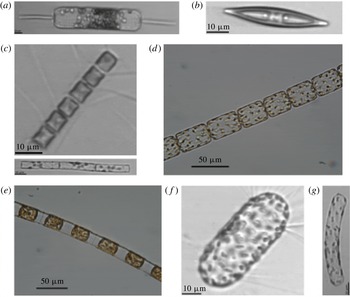
The behaviour of suspended particles in turbulent flows is of considerable interest to a variety of processes, including dispersion of aerosols and collisions of water droplets in the atmosphere, dispersions of oil spills treated with dispersants, sediment transport and ecological processes in the plankton (see e.g. Guazzelli & Morris Reference Guazzelli and Morris2011). The latter is perhaps the least familiar to fluid dynamicists, but is of great importance because of the key roles plankton play in oceanic food webs, sustaining all the world’s commercially important fisheries, and in global biogeochemical cycles, particularly the carbon cycle. Our interest here is in the behaviour of diatoms in turbulent flows. Diatoms are one of the largest and most significant groups of photosynthetic planktonic organisms in coastal and high-latitude environments. They are unicellular, but many species form colonies, often in the form of long chains and filaments, as shown in figure 1, making them an attractive model for studies on non-spherical particles in environmental turbulent flows. Diatoms are non-motile but they possess a siliceous cell wall that is denser than seawater (Eppley, Holmes & Strickland Reference Eppley, Holmes and Strickland1967), causing cells to be, generally, negatively buoyant. From an ecological perspective, sinking velocities and trajectories of diatoms in the upper mixed layer of the ocean are of a great interest, because of their effect on encounter-based processes in the plankton (e.g., prey–predator interactions, aggregate formation) and because the sedimentation of diatoms (as individuals or in aggregates) contributes to the shunting of
 $\text{CO}_{2}$
from the atmosphere into the deep ocean where it gets sequestered for thousands of years.
A mosaic of images of diatoms taken with a light microscope (d and e) or an Imaging Flow cytometer (a, b, c, f and g). (a) Ditylum brightwellii (b) Navicula sp. (c) Chaetoceros sp. (a chain-forming diatom), (d) Lauderia annulata (a chain-forming diatom), (e) Lithodesmium undulatum (a chain-forming diatom), (f) Chorethron sp., and (g) Cylindrotheca sp.

Sinking rates of diatoms have been largely measured in quiescent water (Smayda Reference Smayda1970), while in the surface layer of the ocean, where diatom reside, shear stresses applied by wind, breaking waves and thermal instabilities induce turbulence (Gerbi et al. Reference Gerbi, Trowbridge, Terray, Plueddemann and Kukulka2009). Diatoms are typically smaller than or of the same size as the Kolmogorov length scale (Karp-Boss & Jumars Reference Karp-Boss and Jumars1998; Barton et al. Reference Barton, Ward, Williams and Follows2014), hence our interest is in turbulence at the dissipation scale, which is supposedly independent of the production mechanism. Early observations that diatoms thrive in turbulence (Margalef Reference Margalef1978) and that stirring of cultures keeps cells in suspension lead to the notion that turbulence helps keep phytoplankton suspended and increases their residence time in the sun-lit surface layer of the ocean. Intriguing laboratory observations, however, suggest that turbulence enhances sinking velocities of at least some species of phytoplankton, including diatoms, relative to their still-water velocities (Ruiz, Macías & Peters Reference Ruiz, Macías and Peters2004), but mechanisms remain illusive. Ruiz et al. (Reference Ruiz, Macías and Peters2004) proposed differential concentration as the mechanisms for the observed altered settling velocities, but this mechanism invoked results from systems with particles that are drastically different from diatoms (Wang & Maxey Reference Wang and Maxey1993; Wang & Stock Reference Wang and Stock1993). Differential concentration in these studies is induced by particle inertia, leading to particle concentration in regions of downwardly moving fluid; however, diatoms and other phytoplankton are weakly inertial to follow the same physical mechanism.
Here we use a numerical model to examine whether rotation and orientation of diatoms in a turbulent flow can result in biased trajectories, enhanced sinking and preferential concentrations. While diatom morphologies are complex and may include spines and other projections (see figure 1), Nguyen et al. (Reference Nguyen, Karp-Boss, Jumars and Fauci2011) showed that in a simple shear flow the motion of a diatom with spines or projections could be well predicted from the theory of the motion of spheroids in a simple shear flow, providing that the cell is described by the smallest inscribing spheroid that encompasses both the cell and its spines. In a steady shear flow, a prolate spheroid spends most of its time aligned with the velocity vectors and tumbles with a predictable frequency that is a function of its aspect ratio and the magnitude of the shear rate (Jeffery Reference Jeffery1922). Observations on the motion of rigid diatom chains in a Couette flow show that they undergo periodic rotation, as predicted by theory (Jeffery Reference Jeffery1922), with a period that increases with increasing chain aspect ratio (Karp-Boss & Jumars Reference Karp-Boss and Jumars1998). In unsteady shear and fully developed turbulent flows, the motion of axisymmetric particles becomes more complex, but a growing number of studies have advanced our understanding of the translation, rotation and orientation of dilute suspensions of small spheroids and fibres in turbulence, highlighting the rich dynamics of interactions (see the recent review by Voth & Soldati Reference Voth and Soldati2017). Important insights about the motion of neutrally buoyant rigid fibres in turbulence came from a study by Olson & Kerekes (Reference Olson and Kerekes1998). These authors used analytical approximations to derive translational and rotational dispersion coefficients for fibres in an isotropic stochastic flow field and showed a strong dependence of these coefficients on the fibre length. Using direct numerical simulations, Shin & Koch (Reference Shin and Koch2005) studied the translational and rotational motions of neutrally buoyant slender fibres in fully developed isotropic turbulence. Particles in their simulations ranged in size from tracer-like particles to fibres that are larger than the Kolmogorov scale. Their results show that fibres that are much smaller than the Kolmogorov length scale act as flow tracers and rotate like material lines. With increasing length the fibre rotation rate attenuates as it becomes insensitive to the eddies that are smaller than the fibre length. The assuagement of the rotation rate was shown later to be associated with the tendency of rod-like particles to align more strongly with the vorticity vector than with the principal axis of strain (Pumir & Wilkinson Reference Pumir and Wilkinson2011). Experimental measurements of rotation rates along the trajectories of short nylon threads in a turbulent flow are in agreement with model results (Parsa et al. Reference Parsa, Calzavarini, Toschi and Voth2012). Several studies have followed since, expanding the parameter space of this problem (e.g. Andersson, Zhao & Barri Reference Andersson, Zhao and Barri2012; Parsa & Voth Reference Parsa and Voth2014; Byron et al. Reference Byron, Einarsson, Gustavsson, Voth, Mehlig and Variano2015; Ni et al. Reference Ni, Kramel, Ouellette and Voth2015). A common observation of these studies is the strong preferential alignment of anisotropic particles, either with the direction of the mean flow near a wall in turbulent channel flows (Zhang et al. Reference Zhang, Ahmadi, Fan and McLaughlin2001; Marchioli, Fantoni & Soldati Reference Marchioli, Fantoni and Soldati2010) or with the local velocity gradient tensor in isotropic turbulence, subsequently affecting rotational and translational motions.
The studies described above considered neutrally buoyant particles. For particles denser than the carrying fluid the presence of gravity adds further complication to the dynamics. The case of slender fibres sedimenting in a quiescent fluid has been the subject of many studies, see the review by Guazzelli & Hinch (Reference Guazzelli and Hinch2011). Most of these studies investigate the dilute regime, numerically (Mackaplow & Shaqfeh Reference Mackaplow and Shaqfeh1998; Butler & Shaqfeh Reference Butler and Shaqfeh2002; Gustavsson & Tornberg Reference Gustavsson and Tornberg2009), whereas both dilute and semi-dilute regimes have been examined experimentally (e.g. Herzhaft et al. Reference Herzhaft, Guazzelli, Mackaplow and Shaqfeh1996; Herzhaft & Guazzelli Reference Herzhaft and Guazzelli1999). The results show that in the dilute regime, a suspension loses its homogeneity, forming packets that are separated by sparse regions. In this regime the mean sedimentation velocity increases compared to the maximum velocity of an isolated fibre. In the semi-dilute regime, however, hindrance effects reduce mean velocity and the effect is stronger for a suspension of fibres than for a suspension of spheres. In both regimes the fibres are observed to orient in the direction of gravity (Herzhaft & Guazzelli Reference Herzhaft and Guazzelli1999). Fewer studies have examined the problem of anisotropic particles settling in an external flow (i.e. not induced by the motion of the particles). Earlier studies have considered a cellular flow field and showed enhanced sedimentation of spheroids compared to spheres, and that at large aspect ratios tumbling become chaotic (Mallier & Maxey Reference Mallier and Maxey1991; Shin & Maxey Reference Shin and Maxey1997). Siewert et al. (Reference Siewert, Kunnen, Meinke and Schröder2014) used direct numerial simulations to study settling velocities of heavy ellipsoids in decaying isotropic turbulence. They found a preferential orientation with respect to the direction of gravity for prolate and oblate ellipsoids and a higher sedimentation velocity than that calculated from the orientation probabilities. Their study demonstrated that non-spherical, inertial particles experience a preferential sweeping mechanism, as was previously demonstrated for spheres (Wang & Maxey Reference Wang and Maxey1993; Toschi & Bodenschatz Reference Toschi and Bodenschatz2009; Gustavsson, Vajedi & Mehlig Reference Gustavsson, Vajedi and Mehlig2014; Bec, Homann & Ray Reference Bec, Homann and Ray2014). The effect of turbulence on the settling of spheroids was found to be dependent on the turbulence level and the aspect ratio of the spheroid (see Siewert et al. Reference Siewert, Kunnen, Meinke and Schröder2014). In that study, all parameters were chosen to match ice particles in turbulent clouds, where the inertia of the particles is high. Diatoms and other phytoplankton represent the other extreme, anisotropic particles that are weakly inertial. Here we expand modelling efforts to the parameter space at which phytoplankton operate (see the Appendix).
We model diatom chains as prolate spheroids, using analytical and direct numerical simulations to examine if mean settling velocities of inertia-less diatoms are altered by turbulence. We begin by introducing the flow solver and the one-way coupling model used in this study to describe the particle motion in homogenous isotropic turbulence § 2. Next, we examine whether turbulence affects sinking velocities and clustering of weakly inertial prolate spheroids, and how this may vary as a function of different particle parameters (§ 3). Alteration of sinking velocities is explained further in this section, considering a simple shear flow. The main conclusions and final remarks are drawn in § 4.
2 Governing equations and numerical method
2.1 Fluid phase
The incompressible turbulent velocity field,
 $\boldsymbol{u}$
, obeys the Navier–Stokes and continuity equations:
 $$\begin{eqnarray}\displaystyle & \displaystyle \frac{\unicode[STIX]{x2202}\boldsymbol{u}}{\unicode[STIX]{x2202}t}+\boldsymbol{u}\boldsymbol{\cdot }\unicode[STIX]{x1D735}\boldsymbol{u}=-\unicode[STIX]{x1D735}p+\frac{1}{Re}\unicode[STIX]{x1D6FB}^{2}\boldsymbol{u}+\boldsymbol{f}, & \displaystyle\end{eqnarray}$$
 $$\begin{eqnarray}\displaystyle & \displaystyle \unicode[STIX]{x1D735}\boldsymbol{\cdot }\boldsymbol{u}=0. & \displaystyle\end{eqnarray}$$
Here
 $t$
denotes the time,
 $p$
the pressure,
 $Re$
the Reynolds number and
 $\boldsymbol{f}$
the random forcing field necessary to maintain the turbulent velocity in a statistically steady state. The equations are discretized in a cubic domain with periodic conditions at the boundaries. We employ direct numerical simulation (DNS) to solve all the relevant flow scales without any artificial model at the smallest scales. Since we evolve the equations in a three-periodic domain, it is natural to do so in Fourier space with a pseudo-spectral method. In this numerical scheme the nonlinear terms are evaluated in physical space using the classic
 $2/3$
rule to minimize aliasing error. Time integration is performed with a third-order, low-storage Runge–Kutta method where the diffusive terms are analytically calculated (note that in Fourier space the Laplacian operator is proportional to the square of the modulus of the wave vector
 $k^{2}$
) while an Adam–Bashforth-like approximation is employed for the nonlinear terms (Rogallo Reference Rogallo1981). The stochastic forcing is evaluated in Fourier space and acts isotropically on the first shell of wave vectors. The forcing amplitude is constant in time and the field is delta-correlated in time and uniformly distributed in phase and directions (Vincent & Meneguzzi Reference Vincent and Meneguzzi1994). We employed a resolution of
 $128^{3}$
grid points with a Taylor Reynolds number
 $Re_{\unicode[STIX]{x1D706}}=100$
and
 $64^{3}$
grid points with a Taylor Reynolds number
 $Re_{\unicode[STIX]{x1D706}}=60$
. The turbulence is characterized by the Taylor Reynolds number
 $Re_{\unicode[STIX]{x1D706}}\equiv u^{\prime }\unicode[STIX]{x1D706}/\unicode[STIX]{x1D708}$
, where
 $u^{\prime }$
is the root-mean-square of velocity fluctuations,
 $\unicode[STIX]{x1D708}$
is the kinematic viscosity and
 $\unicode[STIX]{x1D706}$
is the Taylor microscale,
 $\unicode[STIX]{x1D706}\equiv \sqrt{\unicode[STIX]{x1D716}/15\unicode[STIX]{x1D708}u^{\prime 2}}$
, with
 $\unicode[STIX]{x1D716}$
the kinetic energy dissipation rate. The resolution was chosen so that the velocity gradients are well resolved since they drive the the equation of motion of the particles. Particle statistics are computed from independent samples separated by
 $1.6$
turbulent Kolmogorov time scales,
 $\unicode[STIX]{x1D70F}_{f}\equiv \sqrt{\unicode[STIX]{x1D708}/\unicode[STIX]{x1D716}}$
, corresponding to about
 $300$
configurations per particle. The numerical code has been already employed to study gyrotactic micro-organisms in homogeneous turbulence (Zhan et al.
Reference Zhan, Sardina, Lushi and Brandt2014) and rain droplet evaporation in clouds (Sardina et al.
Reference Sardina, Picano, Brandt and Caballero2015).
2.2 Solution of the particle motion
The prolate spheroids studied here are small compared to the Kolmogorov length scale of the turbulence and have densities close to that of the carrier fluid. The translational relaxation time,
 $\unicode[STIX]{x1D70F}_{p}$
, for prolate spheroids, assuming an isotropic particle orientation distribution is given by
 $$\begin{eqnarray}\unicode[STIX]{x1D70F}_{p}=\frac{2\unicode[STIX]{x1D70C}_{p}a^{2}}{9\unicode[STIX]{x1D707}_{f}}\frac{{\mathcal{A}}{\mathcal{R}}\ln ({\mathcal{A}}{\mathcal{R}}+\sqrt{{\mathcal{A}}{\mathcal{R}}^{2}-1})}{\sqrt{{\mathcal{A}}{\mathcal{R}}^{2}-1}},\end{eqnarray}$$
with
 $a$
the semi-minor axis of the prolate spheroid and
 ${\mathcal{A}}{\mathcal{R}}$
the aspect ratio (the ratio of polar over equatorial radii of the spheroid) (Shapiro & Goldenberg Reference Shapiro and Goldenberg1993). The time scale for the particles studied here is around three to four orders of magnitude smaller than the relaxation time of the turbulence flow around the particles. Furthermore, rotational relaxation times, concerning spinning and tumbling motions, are reported in the literature to be typically shorter than the translational relaxation time (Zhao et al.
Reference Zhao, Challabotla, Andersson and Variano2015; Marchioli, Zhao & Andersson Reference Marchioli, Zhao and Andersson2016). With these operating parameters a tracer model for the particle motion is a suitable assumption (Shin & Koch Reference Shin and Koch2005; Voth & Soldati Reference Voth and Soldati2017) and we, therefore, assume that the cells behave like passive tracers with a correction given by their Stokes settling velocity.
The particle translational motion obeys
 $$\begin{eqnarray}\displaystyle & \displaystyle \frac{\text{d}\boldsymbol{x}}{\text{d}t}=\boldsymbol{u}|_{x}+\boldsymbol{v}_{s}(\boldsymbol{p}), & \displaystyle\end{eqnarray}$$
 $$\begin{eqnarray}\displaystyle & \displaystyle \boldsymbol{v}_{s}\,(\boldsymbol{p})=v_{s}^{min}\hat{\boldsymbol{e}}_{g}+\left(v_{s}^{max}-v_{s}^{min}\right)\left(\hat{\boldsymbol{e}}_{g}\boldsymbol{\cdot }\boldsymbol{p}\right)\boldsymbol{p}, & \displaystyle\end{eqnarray}$$
with
 $\boldsymbol{x}$
denoting spheroid position,
 $\boldsymbol{u}|_{x}$
the fluid velocity at spheroid position,
 $\boldsymbol{p}$
the spheroid orientation vector,
 $\boldsymbol{v}_{s}$
the Stokes settling velocity and
 $\hat{\boldsymbol{e}}_{g}$
a unit vector in the direction of gravity. Here
 $v_{s}^{min}$
and
 $v_{s}^{max}$
are the minimum and maximum settling speeds in quiescent flow, corresponding to the particles falling with their major axis perpendicular or parallel to the gravity direction. These velocities can be written as
 $$\begin{eqnarray}v_{s}^{max}=\frac{\left(\unicode[STIX]{x1D70C}_{p}-\unicode[STIX]{x1D70C}_{f}\right)gl^{2}}{\unicode[STIX]{x1D707}_{f}}\unicode[STIX]{x1D6FE}_{0}\left({\mathcal{A}}{\mathcal{R}}\right);\quad v_{s}^{min}=\frac{\left(\unicode[STIX]{x1D70C}_{p}-\unicode[STIX]{x1D70C}_{f}\right)gl^{2}}{\unicode[STIX]{x1D707}_{f}}\unicode[STIX]{x1D6FE}_{1}\left({\mathcal{A}}{\mathcal{R}}\right),\end{eqnarray}$$
with
 $g$
the gravitational acceleration,
 $l$
the length of the spheroid’s major axis,
 $\unicode[STIX]{x1D707}_{f}$
the dynamic viscosity of the fluid,
 $\unicode[STIX]{x1D70C}_{p}$
and
 $\unicode[STIX]{x1D70C}_{f}$
the densities of the particle and the fluid. Here
 $\unicode[STIX]{x1D6FE}_{0}$
and
 $\unicode[STIX]{x1D6FE}_{1}$
are functions of the aspect ratio
 ${\mathcal{A}}{\mathcal{R}}$
, whose full expression can be found in Dahlkild (Reference Dahlkild2011) among others.
The spheroid rotation follows the inertialess Jeffery equation
 $$\begin{eqnarray}\frac{\text{d}\boldsymbol{p}}{\text{d}t}=\frac{1}{2}\unicode[STIX]{x1D74E}|_{x}\times \boldsymbol{p}+\unicode[STIX]{x1D6FC}\left[\unicode[STIX]{x1D644}-\boldsymbol{p}\boldsymbol{p}\right]\boldsymbol{\cdot }\unicode[STIX]{x1D640}|_{x}\boldsymbol{\cdot }\boldsymbol{p},\end{eqnarray}$$
with
 $\unicode[STIX]{x1D74E}|_{x}$
the flow vorticity at the particle’s position,
 $\unicode[STIX]{x1D644}$
the second-order identity tensor,
 $\unicode[STIX]{x1D640}|_{x}$
the symmetric part of the velocity deformation tensor and
 $\unicode[STIX]{x1D6FC}$
a function of the spheroid aspect ratio
 ${\mathcal{A}}{\mathcal{R}}$
, defined as
 $$\begin{eqnarray}\unicode[STIX]{x1D6FC}=\frac{{\mathcal{A}}{\mathcal{R}}^{2}-1}{{\mathcal{A}}{\mathcal{R}}^{2}+1}.\end{eqnarray}$$
To solve the equations above, the flow velocity, vorticity and velocity gradients at the particle positions are calculated with a second-order interpolation scheme and a high enough resolution to capture the flow velocity gradients. The same Runge–Kutta scheme used for the carrier phase is employed to perform the time integration of (2.4) and (2.7) with a small enough time step (
 ${\approx}0.001\unicode[STIX]{x1D70F}_{f}$
) to capture the time evolution of particle orientations via a formulation based on quaternions. We evolve a total of
 $200\,000$
spheroids for each simulation.
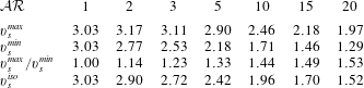
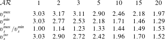
Maximum, minimum and average of settling velocities in quiescent flow, scaled with the Kolmogorov velocity for the investigated cases versus different aspect ratios. Here
 $\unicode[STIX]{x1D70C}_{p}/\unicode[STIX]{x1D70C}_{f}=1.05$
and
 $D_{eq}=\unicode[STIX]{x1D702}/6$
.
3 Results
We first investigate the settling of prolate spheroidal particles of constant volume, focusing on the effect of the particle aspect ratio. The parameters used are
 $Re_{\unicode[STIX]{x1D706}}=100$
,
 $\unicode[STIX]{x1D70C}_{p}/\unicode[STIX]{x1D70C}_{f}=1.05$
and
 $D_{eq}=\unicode[STIX]{x1D702}/6$
, where
 $D_{eq}$
is the diameter of a sphere having the same volume as the prolate spheroid and
 $\unicode[STIX]{x1D702}$
is the Kolmogorov length scale. Fixing the volume, the settling speed varies with the aspect ratio. It should be noted that for the higher-aspect-ratio cases examined here (
 ${\mathcal{A}}{\mathcal{R}}\geqslant 15$
), the larger diameter of the spheroid exceeds the Kolmogorov length scale
 $\unicode[STIX]{x1D702}$
(
 ${\approx}1.24$
for
 ${\mathcal{A}}{\mathcal{R}}=24$
). This does not violate our assumption of a tracer particle since rods act as tracers when their length is less than
 $5\unicode[STIX]{x1D702}$
and deviations from the tracer behaviour are very small until about
 $15\unicode[STIX]{x1D702}$
(Parsa & Voth Reference Parsa and Voth2014). For the simulations presented here, the average settling speed of an uniformly distributed suspension,
 $v_{s}^{iso}$
, varies in the range
 $1.5{-}3u_{\unicode[STIX]{x1D702}}$
. Table 1 shows the settling velocities for the investigated cases. The reported values are all normalized by the Kolmogorov velocity. Note that the average settling speed
 $v_{s}^{iso}$
for spheroids in a quiescent flow is calculated as
 $$\begin{eqnarray}v_{s}^{iso}=\frac{\left(v_{s}^{max}+2v_{s}^{min}\right)}{3},\end{eqnarray}$$
based on the assumption that the orientation of spheroids (cosine of the angle between spheroid’s symmetric axis and the gravity direction) is uniformly distributed.
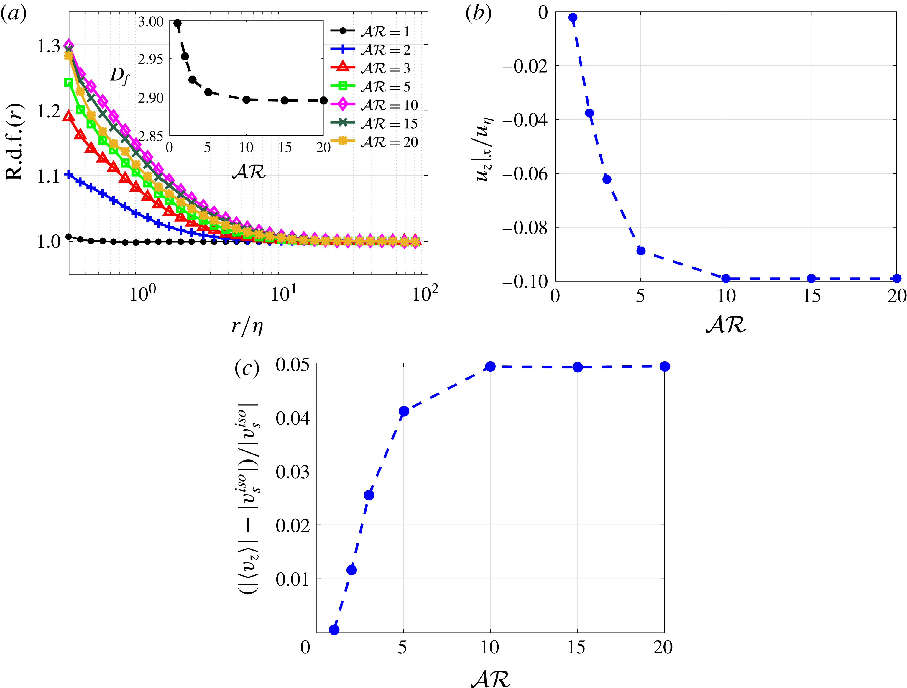
The results of the simulations are shown in figure 2. The main observation is that within the parameter space relevant to diatom chains, settling spheroids weakly cluster (figure 2
a) and preferentially sample regions of downwelling flow, leading to downward velocity biases of up to
 $10\,\%$
of the Kolmogorov velocity
 $u_{\unicode[STIX]{x1D702}}$
(figure 2
b). This corresponds to an increase of the mean settling speed of about
 $5\,\%$
compared with the mean settling speed in quiescent fluid (figure 2
c). These effects increase with the aspect ratio,
 ${\mathcal{A}}{\mathcal{R}}$
, and saturate for
 ${\mathcal{A}}{\mathcal{R}}\geqslant 10$
. In studies regarding unstable settling suspensions (Koch & Shaqfeh Reference Koch and Shaqfeh1989; Herzhaft et al.
Reference Herzhaft, Guazzelli, Mackaplow and Shaqfeh1996; Mackaplow & Shaqfeh Reference Mackaplow and Shaqfeh1998; Herzhaft & Guazzelli Reference Herzhaft and Guazzelli1999), the enhanced sedimentation velocity is explained by two mechanisms. First, the preferential concentration in downwelling flow (as also observed in this study) and, second, the preferred orientation parallel to the gravity direction that causes fibres to settle faster. In these studies, the velocity disturbances due to the settling particles produce vertical shearing motion, which causes the preferential orientation. In the present study, however, the turbulent flow remains isotropic due to the one-way coupling assumption and the second effect cannot observed. Therefore, the increase in the settling speed can be only attributed to preferential sampling of regions with downwelling flow.
(a) Radial distribution function of particle positions; the inset in this panel reports the fractal dimension of the clustering, estimated by fitting the r.d.f. with a power-law in the range
 $r/\unicode[STIX]{x1D702}=[0.2:2]$
, (b) average of fluid vertical velocity at the particle position and (c) increase in the settling velocity (difference in the settling rate with respect to the quiescent settling average
 $v_{s}^{iso}$
, normalized by
 $v_{s}^{iso}$
).

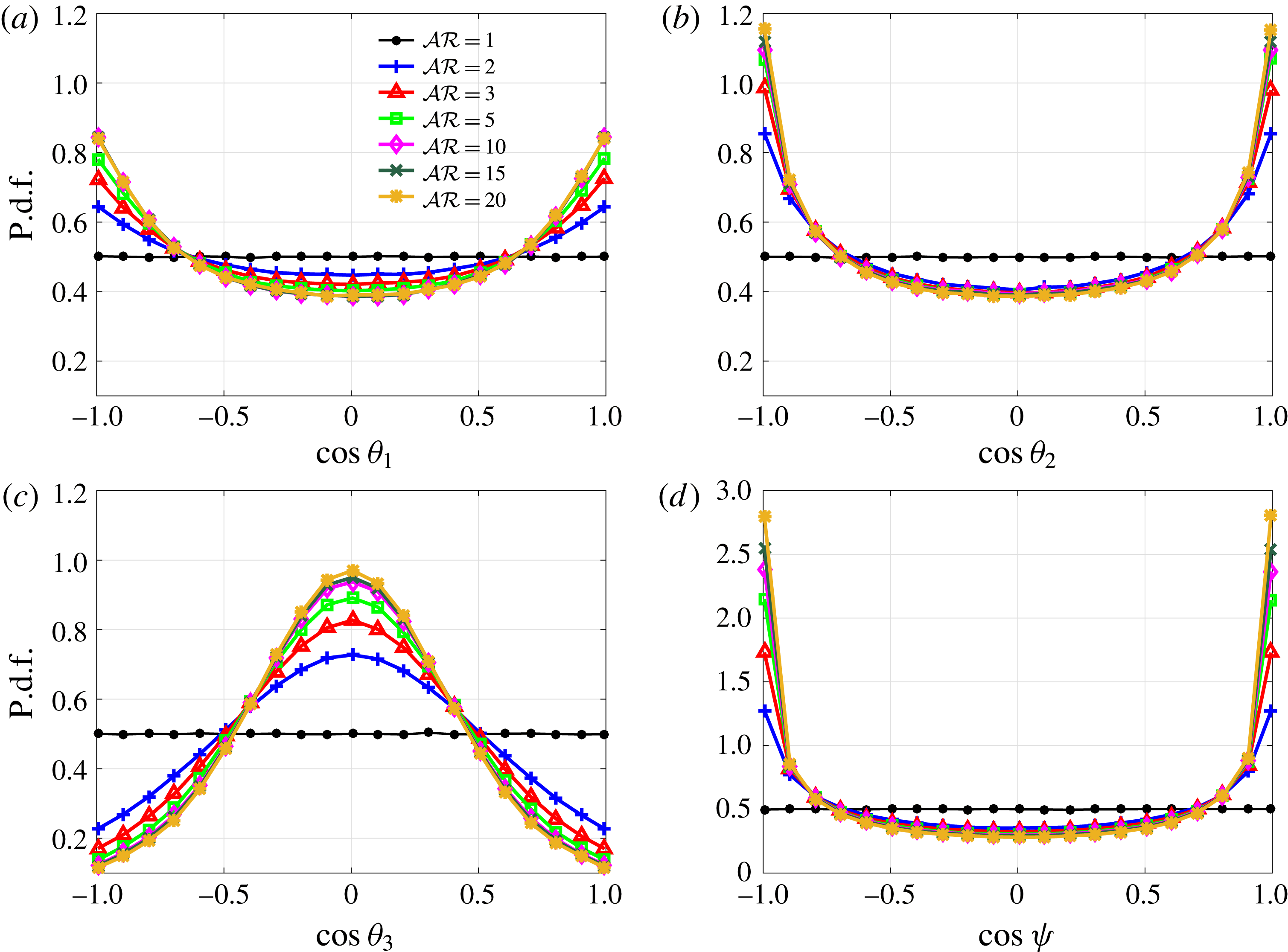
Probability density function (p.d.f.) of orientation of particles with different aspect ratios with respect to the three eigenvectors of the deformation tensor (a–c) and the local vorticity vector (d).

To quantify patchiness (clustering) in fully three-dimensional isotropic turbulent flows, we use the radial pair distribution function (r.d.f.), sometimes also called the correlation function. The r.d.f. measures the probability of finding a particle pair separated by a given radial distance, normalized by the value expected from a uniform distribution. This is defined as
 $$\begin{eqnarray}g\left(r\right)=\frac{1}{4\unicode[STIX]{x03C0}r^{2}}\frac{\text{d}N_{r}}{\text{d}r}\frac{1}{n_{0}},\end{eqnarray}$$
where
 $n_{0}=0.5N_{p}(N_{p}-1)/V_{0}$
is the density of pairs in the whole volume
 $V_{0}$
.
 $N_{p}$
is the total number of particles in the domain and
 $N_{r}$
is the number of pairs at distance
 $r$
. The small volume fraction, used here, removes the exclusion effects, and thus an r.d.f. for a random distribution results in a flat value of
 $1$
. The r.d.f. is reported in figure 2(a). In the inset of the same figure, we report the scaling exponent of the r.d.f. at small separations, also often used as an indicator of patchiness (Durham et al.
Reference Durham, Climent, Barry, De Lillo, Boffetta, Cencini and Stocker2013). This exponent denotes the fractal dimension of the set where particles are found. Patchiness is seen to increase with the particle aspect ratio and saturate at the largest values considered. However, a fractal dimension
 $2.9$
shows weak clustering. Increasing the aspect ratio, while keeping the volume and the density ratio constant, changes the average settling speed,
 $v_{s}^{iso}$
, and the ratio between maximum and minimum settling speed,
 $v_{s}^{max}/v_{s}^{min}$
, simultaneously. Therefore the saturation in the patchiness and the preferential sampling of regions of downwelling flow can be explained by the change in
 $v_{s}^{iso}$
and
 $v_{s}^{max}/v_{s}^{min}$
. A detailed study of each effect is given in the next subsection.
In figure 3, we study the relation between particle orientation and the underlying flow field when varying the particle shape. In figure 3(a–c), we show the orientation of the particle with respect to the three eigendirections of the strain tensor, defined such that
 $\unicode[STIX]{x1D706}_{1}>\unicode[STIX]{x1D706}_{2}>\unicode[STIX]{x1D706}_{3}$
so that the first eigendirection is extensional and the third eigendirection is compressional. The angles between the eigendirections and the spheroid orientation are denoted as
 $\unicode[STIX]{x1D703}_{1}$
,
 $\unicode[STIX]{x1D703}_{2}$
and
 $\unicode[STIX]{x1D703}_{3}$
. In figure 3(d), we show
 $\unicode[STIX]{x1D713}$
, the angle between the orientation and the local vorticity vector. While spherical particles,
 ${\mathcal{A}}{\mathcal{R}}=1$
, are isotropic in nature, elongated spheroids tend to align with the local flow strain, more frequently with the second eigendirection, and with the local flow vorticity. Indeed, the p.d.f.s peak when prolate particles are parallel to the eigendirections associated with
 $\unicode[STIX]{x1D706}_{2}$
and
 $\unicode[STIX]{x1D706}_{1}$
. An increasing probability of parallel alignment with the first two eigendirections of the strain is seen with increased aspect ratio. The spheroid is most likely to be normal to the third eigendirection of the strain, as shown in figure 3(c). The strongest tendency to align with the local vorticity vector is consistent with previous observations for neutrally buoyant spheroids (Chevillard & Meneveau Reference Chevillard and Meneveau2013; Ni et al.
Reference Ni, Kramel, Ouellette and Voth2015). The alignment with the vorticity vector increases with the aspect ratio
 ${\mathcal{A}}{\mathcal{R}}$
.
3.1 Numerical experiments
The parameters that define the behaviour of the particles in this regime are the ratio of the amplitude of the sedimenting velocity and the Kolmogorv velocity scale of the turbulence,
 $v_{s}^{iso}/u_{\unicode[STIX]{x1D702}}$
and the aspect ratio
 ${\mathcal{A}}{\mathcal{R}}$
. However, increasing the aspect ratio, while maintaining the mass constant, simultaneously changes the the average settling speed,
 $v_{s}^{iso}$
, and the ratio between maximum and minimum settling speed,
 $v_{s}^{max}/v_{s}^{min}$
. In other words, changing the aspect ratio can affect the results by affecting the rotational motion and also by changing sedimentation trajectories. To disentangle these different effects, we perform a series of numerical experiments to investigate separately the effect of the aspect ratio,
 ${\mathcal{A}}{\mathcal{R}}$
, the amplitude of the sedimenting velocity
 $v_{s}^{iso}$
and the ratio between the maximum (spheroid aligned with the gravity direction) and minimum (normal to gravity) settling speed
 $v_{s}^{max}/v_{s}^{min}$
. In each series of simulations we fix all the parameters except for one to focus on a single parameter effect. While varying only one parameter can result in unrealistic conditions occasionally, it sheds light on the isolated effect of the parameter of interest on particles’ collective behaviour. Since phytoplankton exhibits a striking diversity of cell shapes and characteristics, their kinematics can be influenced in important ways, i.e. their characteristics might change their kinematics in a way that these effects get disentangled from each other. For example, an organism that resists falling in a certain direction can increase the drag anisotropy independently of the aspect ratio.
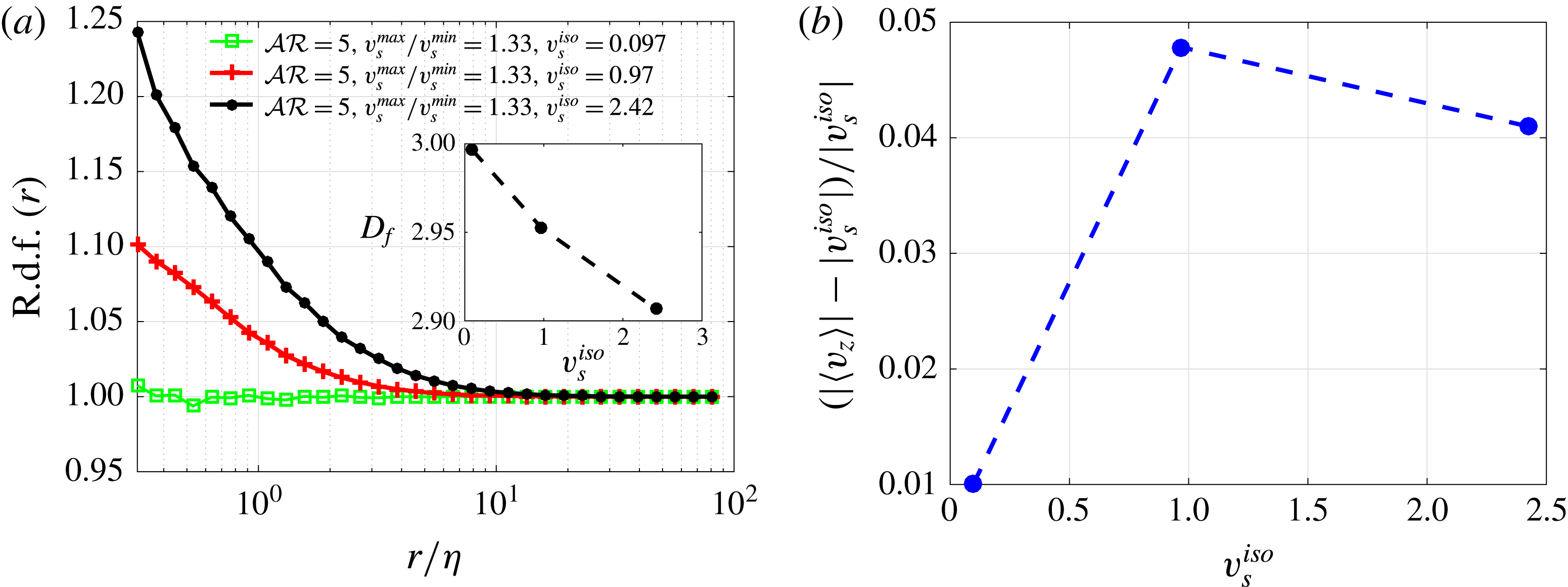
(a) Radial distribution function of particle positions and (b) increase in the settling velocity for
 ${\mathcal{A}}{\mathcal{R}}=5$
and the indicated values of
 $v_{s}^{iso}$
. Here
 $v_{s}^{iso}$
is normalized by the Kolmogorov velocity
 $u_{\unicode[STIX]{x1D702}}$
.

3.1.1 Effect of sedimenting velocity magnitude
First we examine how particle clustering varies with the amplitude of the settling speed. To this end, we keep the aspect ratio
 ${\mathcal{A}}{\mathcal{R}}=5$
, corresponding to a ratio between maximum and minimum settling speed,
 $v_{s}^{max}/v_{s}^{min}=1.33$
, and change
 $v_{s}^{iso}$
from 0.1 to about 2.5 Kolmogorov velocities (this may correspond to a change in the particle size with respect to the turbulence Kolmogorov scale or a change in particle density). Results in figure 4(a) show that patchiness increases with the average settling speed, as measured by the r.d.f. or by the fractal dimension (inset in figure 4
a). The increased clustering, however, does not correspond to an increase of the relative average settling speed when
 $v_{s}^{iso}$
is greater than the Kolmogorov velocity.
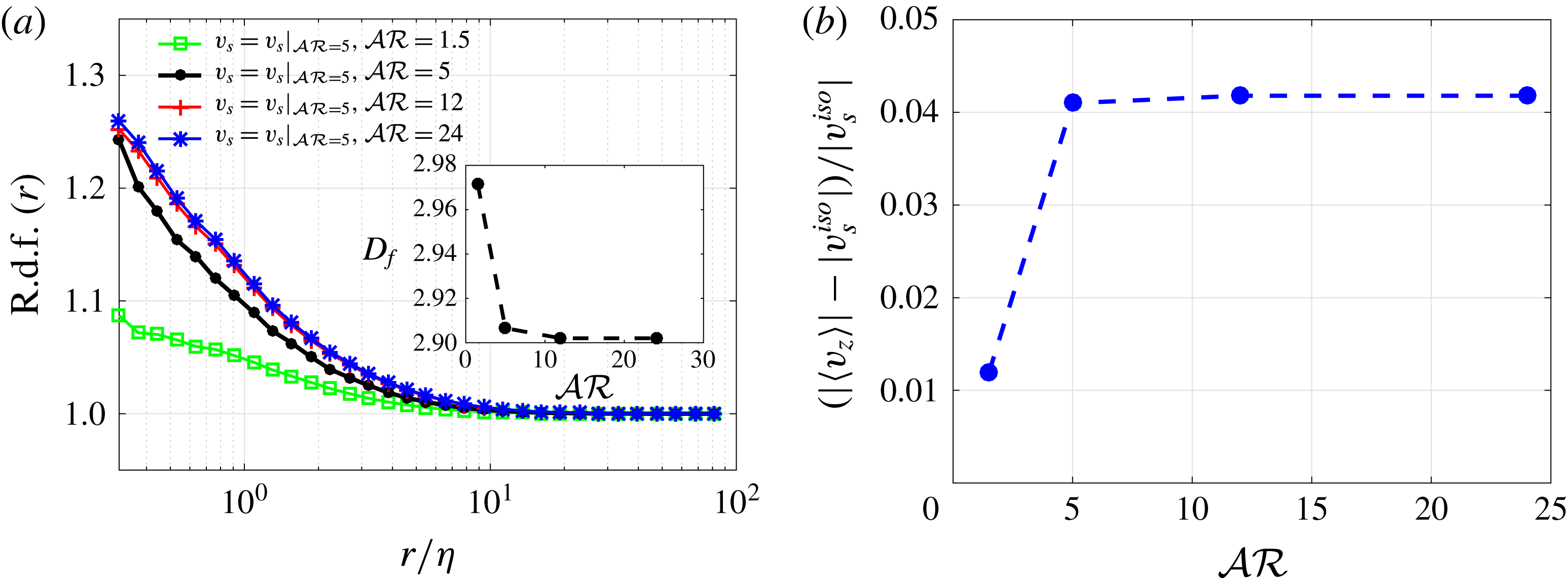
(a) Radial distribution function of particle positions and (b) increase in the settling velocity for the different aspect ratios indicated, while keeping the same maximum and minimum settling speed.

3.1.2 Effect of aspect ratio
To elucidate the role of the particle rotation rate on the observed preferential sampling, we vary
 ${\mathcal{A}}{\mathcal{R}}$
, while artificially keeping the settling speed fixed, both the components parallel and normal to gravity, at the values corresponding to
 $AR=5$
in table 1. The solution of Jeffery’s equation (2.7) reveals that the time spent aligned with the local shear increases with increasing aspect ratio. The results, displayed in figure 5, show that the r.d.f. and the relative increase of sedimenting velocity saturate for
 ${\mathcal{A}}{\mathcal{R}}\geqslant 5$
. Interestingly, rotation rates of oblate and prolate particles are seen to saturate for
 ${\mathcal{A}}{\mathcal{R}}>5$
and for
 ${\mathcal{A}}{\mathcal{R}}<1/5$
in the study of Byron et al. (Reference Byron, Einarsson, Gustavsson, Voth, Mehlig and Variano2015). We have also observed, not shown here, that the alignment with the local vorticity increases with the aspect ratio and saturates when
 ${\mathcal{A}}{\mathcal{R}}\geqslant 5$
unlike the cases in figure 3, where it continues to increase; this suggests that the alignment with vorticity is influenced by the difference between settling parallel and normal to gravity, which is fixed here.
3.1.3 Effect of local alignment
As the alignment with the vorticity vector increases with the aspect ratio
 ${\mathcal{A}}{\mathcal{R}}$
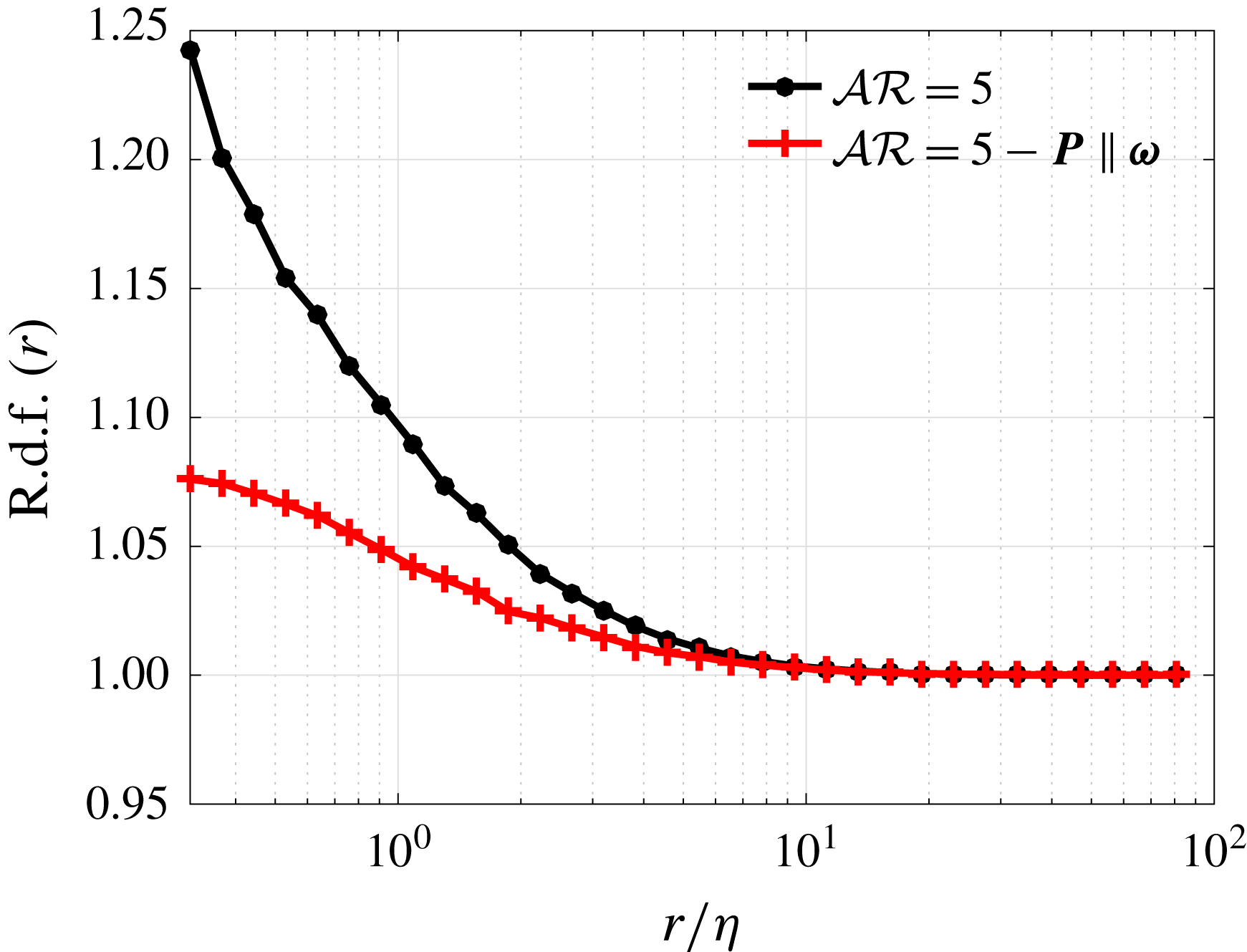
, see figure 3(d), it is interesting to further explore if preferential alignment contributes to biased sampling and clustering of particles. To show the isolated effect of particle alignment with the local vorticity vector we performed a simulation forcing the elongated spheroid to be always aligned with the local vorticity (figure 6): we observe that clustering decreases in comparison to the case in which the particle was free to rotate. We therefore conclude that clustering cannot be explained by the alignment with the local flow vorticity alone.
Radial distribution function of particle positions for particles with
 ${\mathcal{A}}{\mathcal{R}}=5$
and particles with the same sedimenting velocity but with their orientation forced to be always aligned with the local vorticity vector.

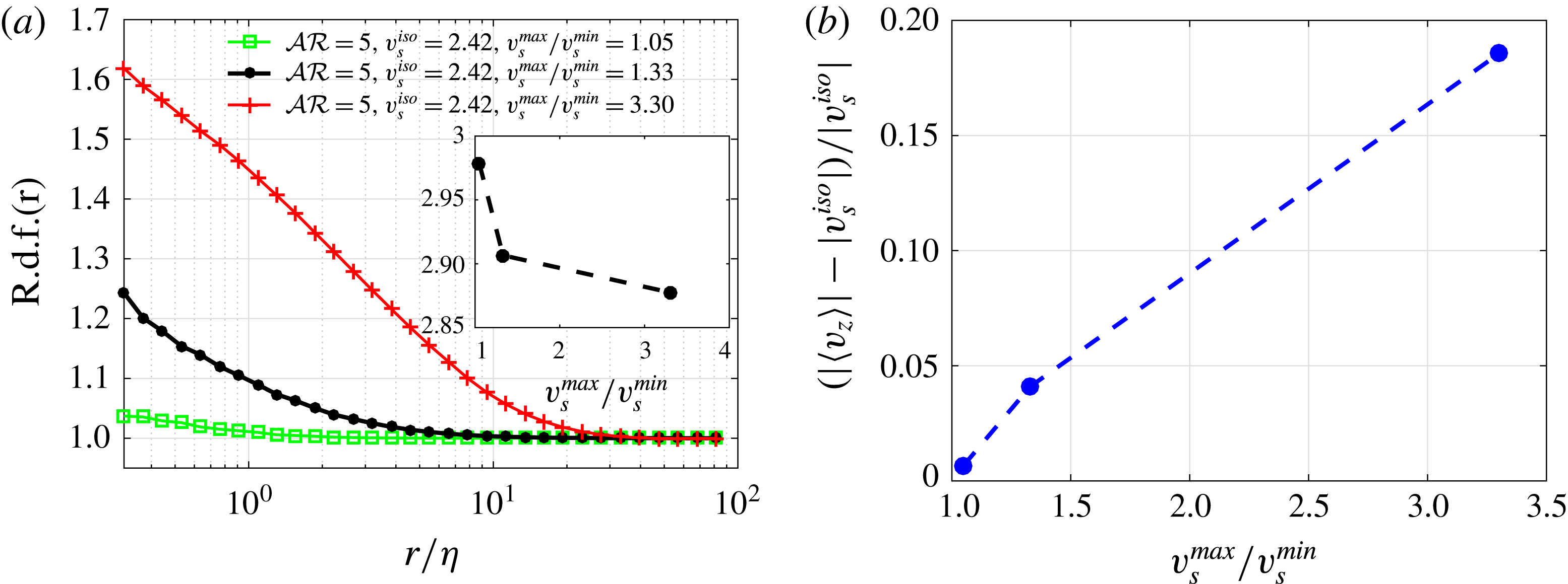
(a) Radial distribution function of particle positions and (b) increase in the settling velocity for settling spheroids with aspect ratio
 ${\mathcal{A}}{\mathcal{R}}=5$
, fixed average settling speed
 $v_{s}^{iso}=2.42$
and different ratios between settling speed in the direction normal and parallel to gravity,
 $v_{s}^{max}/v_{s}^{min}$
, as indicated in the legend. Here
 $v_{s}^{iso}$
is normalized by the Kolmogorov velocity
 $u_{\unicode[STIX]{x1D702}}$
.

Plot of
 $v_{s}^{max}/v_{s}^{min}$
versus
 ${\mathcal{A}}{\mathcal{R}}$
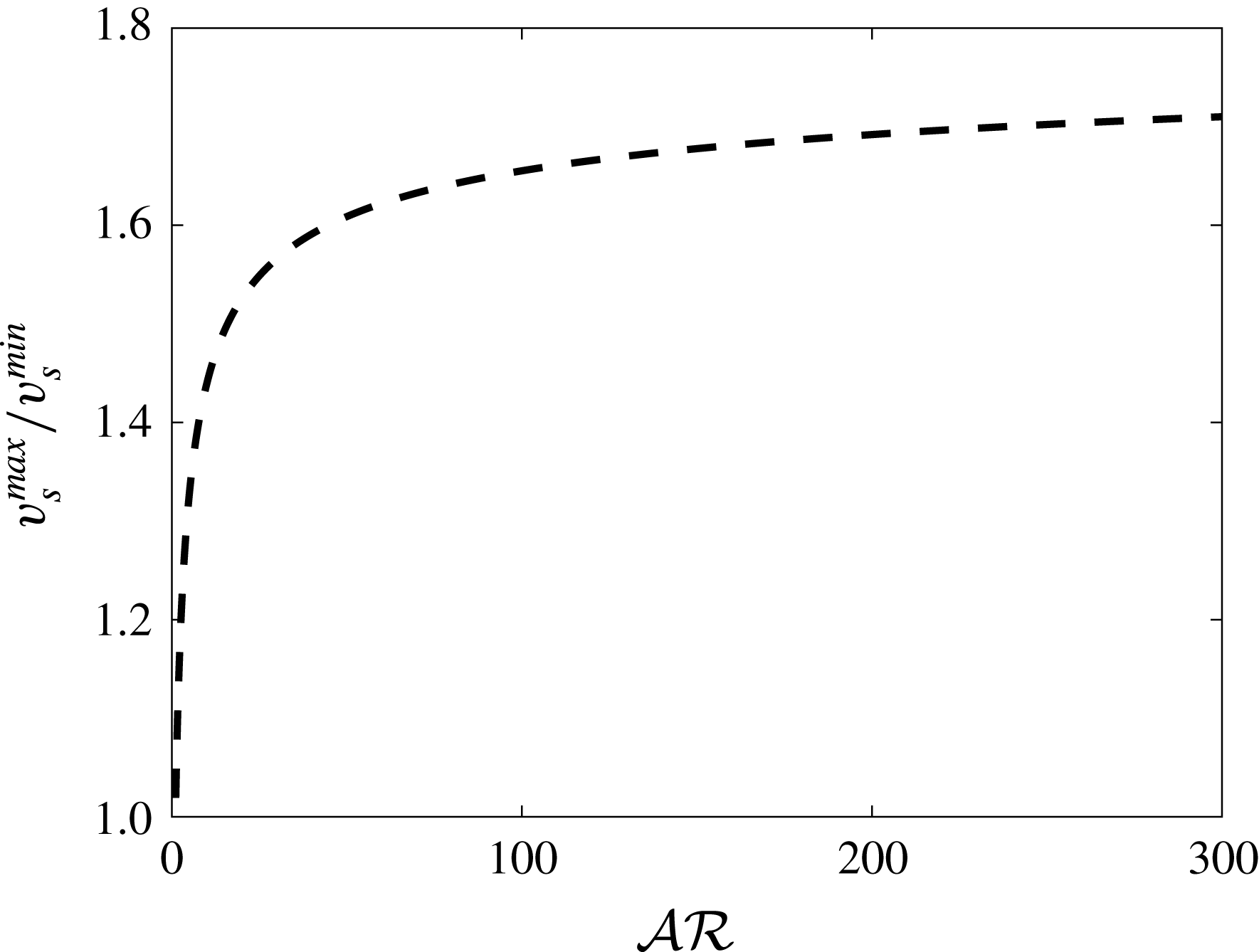
for prolate particles, see e.g. analytical expressions reported in Dahlkild (Reference Dahlkild2011).

3.1.4 Effect of drag anisotropy
One important feature of non-spherical particles in inertialess flows is their drag anisotropy, which can also be exploited by micro-organisms for locomotion. In the case of settling prolate spheroids, this anisotropy is seen in the oblique settling of inclined particles and in the difference between settling speed when oriented parallel or normal to gravity. For the results presented so far we followed the analytical expression for the settling speed derived for prolate spheroids. Shapes in nature are, however, more complicated. Flexibility and non-uniformly distributed mass are likely to cause deviation from the idealized case. To understand more the relevance of drag anisotropy we perform simulations of spheroids with aspect ratio
 ${\mathcal{A}}{\mathcal{R}}=5$
and fixed average settling speed
 $v_{s}^{iso}=2.42$
, while varying the ratio between settling speed in the direction normal and parallel to gravity,
 $v_{s}^{max}/v_{s}^{min}$
. As seen in figure 7(a) clustering increases significantly with drag anisotropy, or
 $v_{s}^{max}/v_{s}^{min}$
. More interestingly, the relative settling speed increases by up to about
 $20\,\%$
when
 $v_{s}^{max}/v_{s}^{min}=3.3$
. The value
 $3.3$
is chosen to artificially emphasize the drag anisotropy effect; note that the ratio between maximum and minimum settling speed of spheroidal particles increases with the aspect ratio and saturates at about
 $1.75$
(figure 8).
3.2 Mechanism for increased settling speed
To understand why ellipsoidal particles preferentially locate in regions of downwelling flow and thus have an enhanced settling speed, we consider a vertical linear shear,
 $\boldsymbol{u}=-\unicode[STIX]{x1D6FE}x\hat{\boldsymbol{e}}_{g}$
with motion constrained to the
 $x$
–
 $z$
plane. We define
 $\unicode[STIX]{x1D703}$
to be the angle the particle symmetry axis makes with the vertical, so that in
 $x$
–
 $z$
co-ordinates the orientation vector is given by
 $\boldsymbol{p}=(\sin \unicode[STIX]{x1D703},\cos \unicode[STIX]{x1D703})^{\text{T}}$
.
From Jeffery’s equation (2.7) the time evolution of particle orientation is given by
 $$\begin{eqnarray}\displaystyle \dot{\unicode[STIX]{x1D703}}=\frac{\unicode[STIX]{x1D6FE}}{2}\left(-1+\unicode[STIX]{x1D6FC}\cos 2\unicode[STIX]{x1D703}\right). & & \displaystyle\end{eqnarray}$$
Note that the particle rotates most slowly when
 $\unicode[STIX]{x1D703}=0$
or
 $\unicode[STIX]{x03C0}$
, and thus spends more time in these states, i.e. aligned with the local shear. From (2.5), the vertical velocity of a particle is given by
 $$\begin{eqnarray}\displaystyle & v_{z}=\unicode[STIX]{x1D6FE}x-v_{s}^{min}-\left(v_{s}^{max}-v_{s}^{min}\right)\cos ^{2}\unicode[STIX]{x1D703}. & \displaystyle\end{eqnarray}$$
The time-averaged vertical velocity over a Jeffery orbit (of duration
 $T=4\unicode[STIX]{x03C0}/\unicode[STIX]{x1D6FE}\sqrt{1-\unicode[STIX]{x1D6FC}^{2}}$
) is given by
 $$\begin{eqnarray}\displaystyle \overline{v_{z}} & = & \displaystyle \frac{1}{T}\int _{0}^{\text{T}}(\unicode[STIX]{x1D6FE}x-v_{s}^{min}-\left(v_{s}^{max}-v_{s}^{min}\right)\cos ^{2}\unicode[STIX]{x1D703})\,\text{d}t\nonumber\\ \displaystyle & = & \displaystyle \unicode[STIX]{x1D6FE}\overline{x}-v_{s}^{min}-\frac{\left(v_{s}^{max}-v_{s}^{min}\right)\sqrt{1-\unicode[STIX]{x1D6FC}^{2}}}{2\unicode[STIX]{x03C0}}\int _{0}^{2\unicode[STIX]{x03C0}}\frac{\cos ^{2}\unicode[STIX]{x1D703}}{-1+\unicode[STIX]{x1D6FC}\cos 2\unicode[STIX]{x1D703}}\,\text{d}\unicode[STIX]{x1D703},\end{eqnarray}$$
where
 $\overline{x}$
is the time-averaged horizontal position. The effect of the shear strength,
 $\unicode[STIX]{x1D6FE}$
, only appears through the term
 $\unicode[STIX]{x1D6FE}\overline{x}$
, and so the effect of the shear on the total vertical velocity of particles can be determined if we know the time-averaged horizontal position. In particular, the only way cells are predicted to exhibit enhanced settling is if they spend more time in downwelling regions.
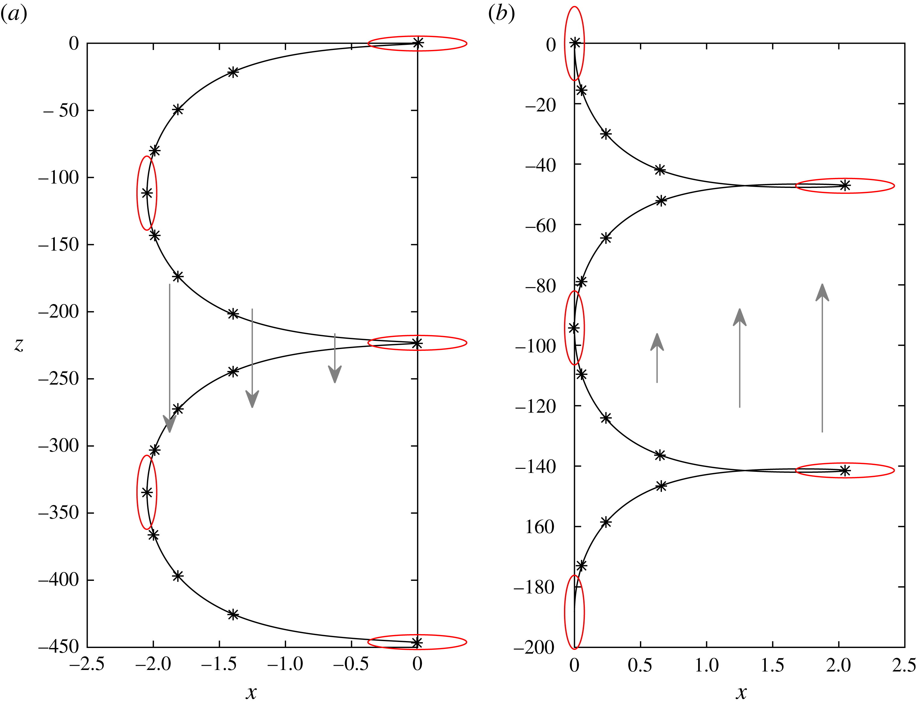
Trajectory of single particle in vertical laminar shear over a Jeffery orbit. Particle initially at the origin with orientation (a)
 $\unicode[STIX]{x1D703}=\unicode[STIX]{x03C0}/2$
and (b)
 $\unicode[STIX]{x1D703}=0$
. Stars indicate position at equally spaced time intervals, red ellipses indicate particle orientation. Grey arrows indicate flow velocity
 $\boldsymbol{u}=-\unicode[STIX]{x1D6FE}x\hat{\boldsymbol{e}}_{g}$
.

To demonstrate how the time-averaged horizontal position is biased towards downwelling regions, yielding enhanced settling, we numerically compute particle trajectories for a complete Jeffery orbit for an example set of parameters taken from table 1:
 $\unicode[STIX]{x1D6FE}=1$
,
 ${\mathcal{A}}{\mathcal{R}}=20$
(
 $\unicode[STIX]{x1D6FC}=0.995$
),
 $v_{s}^{min}=1.29$
and
 $v_{s}^{max}=1.97$
(see figure 9). Particles are initially located at the origin, and the initial orientation is taken as
 $\unicode[STIX]{x1D703}=0$
or
 $\unicode[STIX]{x1D703}=\unicode[STIX]{x03C0}/2$
. Particles initially horizontal (
 $\unicode[STIX]{x1D703}=\unicode[STIX]{x03C0}/2$
, figure 9
a) have a negative horizontal (parallel to the direction of the flow) component due to shear-induced lift, causing them to translate into downwelling flow. As the particle rotates, it reaches a minimum horizontal position at the point when
 $\unicode[STIX]{x1D703}=0$
and then reverses its horizontal component of motion back towards
 $x=0$
which is attained when
 $\unicode[STIX]{x1D703}=3\unicode[STIX]{x03C0}/2$
. The particle has a slowest rotation rate when
 $\unicode[STIX]{x1D703}=0$
or
 $\unicode[STIX]{x03C0}$
, corresponding to the minimum horizontal position, and thus the time-averaged horizontal position is less than the midpoint of the horizontal limits of the trajectory. This bias represents a tendency to cluster in downwelling flow. Particles initially vertical (
 $\unicode[STIX]{x1D703}=0$
, figure 9
b) sediment with a positive horizontal component into upwelling flow. As the particle rotates, it reaches a maximum horizontal position at the point when
 $\unicode[STIX]{x1D703}=3\unicode[STIX]{x03C0}/2$
and then reverses its horizontal component of motion back towards
 $x=0$
, which is attained when
 $\unicode[STIX]{x1D703}=\unicode[STIX]{x03C0}$
. Again, the particle has a slowest rotation rate at the minimum horizontal position (horizontal distance from origin), and thus the time-averaged horizontal position is less than the midpoint of the horizontal limits of the trajectory (horizontal distance from origin is larger). This simple example shows how shear, rotation, lift, and drag-anistropy couple to bias particle trajectories towards downward flow. These simpler model shows that drag anisotropy can increase the bias towards regions of negative fluid velocity, and therefore explains the sensitivity of the results to the ratio between maximum and minimum sedimentation velocity
 $v_{s}^{max}/v_{s}^{min}$
(see § 3.1.4).
Note finally that this mechanism for preferential sampling of downwelling flows is similar to the one reported by Koch & Shaqfeh (Reference Koch and Shaqfeh1989) when studying the instability of a dispersion of sedimenting spheroids. In their study, however, the vertical shearing motion was induced by the velocity disturbance of a neighbouring spheroid while we assume here a constant background shear.
4 Final remarks
We report results from simulations of elongated, rigid particles (prolate spheroids) with different aspect ratios sinking in homogenous, isotropic turbulence. The parameters used in this study represent marine or freshwater diatoms that are characterized by very small relaxation times compared to that of the fluid but with settling velocities on the order of Kolmogorov velocities characteristic of the mixed layer in the ocean. Given the small size of diatoms relative to the Kolmogorov length-scale and their short relaxation time, cells are assumed to behave like passive tracers with a correction given by their Stokes settling velocity. We show that turbulence does increase the settling velocities of inertia-less elongated particles, compared to their Stokes settling velocities, and that the effect increases as the aspect ratio of the particle increases, but saturates at
 ${\mathcal{A}}{\mathcal{R}}\geqslant 10$
. The magnitude of this effect, however, is small (
 ${\sim}5\,\%$
, figure 2
 $c$
). It should be noted that despite the enhanced mean settling velocity for diatoms reported in this study, there could be dispersion of particles in turbulent flow that increases the residence time of some individuals.
Further, we study homogenous isotropic turbulence at the dissipation scale, and thus neglect large-scale turbulence that might play a role in suspending diatoms. Indeed, the question ‘How local enhancement is related to residence time in the mixed layer of the ocean?’ is still unanswered and might be very well related to the large scale turbulence that is not captured in the current model. In our model, turbulence dissipation rate,
 $\unicode[STIX]{x1D716}$
, was set to
 $10^{-6}~\text{m}^{2}~\text{s}^{-3}$
. This choice is within the range observed in the ocean’s surface boundary layer in a coastal environment (Gerbi et al.
Reference Gerbi, Trowbridge, Terray, Plueddemann and Kukulka2009). For this turbulence level, settling is slightly enhanced. Ruiz et al. (Reference Ruiz, Macías and Peters2004) used a Couette device to generate turbulence and showed that sinking speeds of different species of phytoplankton increased significantly (by an order of magnitude for some species) as
 $\unicode[STIX]{x1D716}$
increased from
 $\unicode[STIX]{x1D716}<10^{-6}~\text{m}^{2}~\text{s}^{-3}$
to
 $\unicode[STIX]{x1D716}>10^{-4}~\text{m}^{2}~\text{s}^{-3}$
. They also showed that downward velocities increased as the ratio between the size of the cell (described as equivalent spherical diameter in their study) and the Kolmogorov length-scale increased (Ruiz et al.
Reference Ruiz, Macías and Peters2004).
Here we show that non-random distributions can arise within the parameter space relevant to diatoms, with weak clustering occurring only for non-spherical cells. Preferential sampling of downwelling flow is due to the interactions between shear, particle rotation, drag, and lift. Elongated spheroids tend to align with the local flow strain (more frequently with the second eigen-direction) and with the local flow vorticity, in agreement with previous studies on neutrally buoyant spheroids in homogenous isotropic turbulence (e.g. Ni et al. (Reference Ni, Kramel, Ouellette and Voth2015), Voth & Soldati (Reference Voth and Soldati2017) and references therein). By considering the simple case of one particle sedimenting in linear shear flow we demonstrate that the time-averaged horizontal position of a particle in the flow (over a complete Jeffery orbit) is biased towards downwelling regions. Spheroids with higher average Stokes settling speeds (
 $v_{s}^{iso}$
) show greater tendency to cluster (see figure 4
 $a$
). However, when
 $v_{s}^{iso}$
is greater than the Kolmogorov velocity, the increase in clustering does not correspond to an increase in relative average settling speed. We also show that clustering increases significantly with drag anisotropy (i.e. the ratio
 $v_{s}^{max}/v_{s}^{min}$
) in a way that does not appear to saturate. Drag anisotropy increases with increasing
 ${\mathcal{A}}{\mathcal{R}}$
and forces particles to sample regions of downwelling flow to a further extent, even when the isolated effect of aspect ratio on the rotational motion is saturated.
Mechanisms that affect sinking and dispersion of phytoplankton hold significant implications to carbon and energy fluxes in aquatic systems. Underlying distributions of phytoplankton at the micro-scale are not well understood as we still lack the tools to measure them in the field. Few available observations suggest that at scales of centimeters, the seascape is more heterogeneous than previously thought (Malkiel, Alquaddoomi & Katz Reference Malkiel, Alquaddoomi and Katz1999; Seuront, Schmitt & Lagadeuc Reference Seuront, Schmitt and Lagadeuc2001; Mitchell et al.
Reference Mitchell, Yamazaki, Seuront, Wolk and Li2008) but mechanisms remain poorly understood. This study provides insights into one mechanism by which weak clustering of chains and elongated cells of diatoms can occur at the millimetre to centimetre scale. A typical fractal dimension of
 $2.8{-}2.9$
shows a weak clustering, and it might be that other mechanisms exist behind the clustering that our model cannot capture.
Cell shape is an important morphological trait affecting many aspects in the ecology of phytoplankton (Smayda Reference Smayda1970; Lewis Reference Lewis1976; Sournia Reference Sournia1982; Reynolds Reference Reynolds1989; Reynolds & Irish Reference Reynolds and Irish1997; Karp-Boss & Boss Reference Karp-Boss and Boss2016) and results from our numerical model further highlight the complex interactions of cell shape with ambient flows. Interestingly, the observed increase in settling speeds does not increase indefinitely, and saturates for
 ${\mathcal{A}}{\mathcal{R}}>10$
. Increasing the aspect ratio, while keeping the particle volume and density ratio constant, varies other characteristics of the particle simultaneously. For example, the mean settling speed in quiescent flow decreases as the ratio between maximum (when particle is oriented parallel to the gravity direction) and minimum (when particle is oriented normal to the gravity direction) settling speed increases. We have therefore performed a series of numerical experiments to isolate the effect of the aspect ratio
 ${\mathcal{A}}{\mathcal{R}}$
, the magnitude of settling velocity
 $v_{s}^{iso}$
and the ratio between the maximum and minimum settling speed
 $v_{s}^{max}/v_{s}^{min}$
in quiescent flow. When
 $v_{s}^{iso}$
and
 $v_{s}^{max}/v_{s}^{min}$
are held constant, the increase in clustering and settling speed begins to saturates at
 ${\mathcal{A}}{\mathcal{R}}=5$
. This indicates that the relative enhancement that we observe for ellipsoids with aspect ratios larger than
 $5$
is due to an increase in the ratio between the maximum and minimum settling speed (
 $v_{s}^{max}/v_{s}^{min}$
) that is associated with a change in particle shape (
 ${\mathcal{A}}{\mathcal{R}}$
at constant volume). Interestingly, an analysis of typical aspect ratios among phytoplankton shows a peak in distribution at
 ${\mathcal{A}}{\mathcal{R}}\sim 5$
(Clavano, Boss & Karp-Boss Reference Clavano, Boss and Karp-Boss2007; Karp-Boss & Boss Reference Karp-Boss and Boss2016), but this may be a coincidence because in nature multiple processes (grazing, diffusion, mechanical breakage by shear) act simultaneously as selective pressures on shape and size in phytoplankton (Karp-Boss & Boss Reference Karp-Boss and Boss2016).
The model presented here is an idealized case of turbulence and phytoplankton in the ocean. Direct numerical simulations are computationally expensive and cannot be used to capture the full range of scales characteristic of oceanic turbulence, and are limited to low Reynolds numbers. We consider homogeneous isotropic turbulence, but in the ocean most turbulent mixing occurs near boundaries and is subjected to stratification and vertical shear. It was found, however, that in stratified regions of the ocean, isotropic motions do exist over some range of scale bounded at the lower end by the Kolmogorov length scale, providing that the non-dimensional isotropy parameter
 $I=\unicode[STIX]{x1D716}/\unicode[STIX]{x1D708}N^{2}$
exceeds
 ${\sim}200$
, where
 $\unicode[STIX]{x1D716}$
is the local mean kinetic energy dissipation,
 $\unicode[STIX]{x1D708}$
the kinematic viscosity and
 $N$
the local mean value of the buoyancy frequency (Thorpe Reference Thorpe2007).
Modelling phytoplankton as rigid prolate spheroids with an even distribution of mass is another simplification of the model. Diatoms exhibit complex morphologies (see figure 1) and often bear spines and other cell projections that can alter dynamics in the flow. Another attribute of chain-forming diatoms that is dynamically important is flexural stiffness, as it spans four orders of magnitude between different species (Young Reference Young2011). Variations in rotation rates between rigid and flexible particles were observed in a laboratory setting (Karp-Boss & Jumars Reference Karp-Boss and Jumars1998), and it is likely that rigid and flexible chains will also exhibit different dynamics in turbulence, a subject that requires more investigations in the future.
Acknowledgements
M.N.A., G.S. and L.B. acknowledge support by the European Research Council grant no. ERC-2013-CoG-616186, TRITOS and the Swedish Research Council grant Outstanding Young Researcher to L.B. Computer time is provided by SNIC (Swedish National Infrastructure for Computing). We also acknowledge the support from the COST Action MP1305: Flowing matter, with particular mention to the discussions held during the workshop ‘Microorganisms in Turbulent Flows’, Lorentz Centre, Leiden, the Netherlands. This work is also supported by the National Science Foundation (NSF) grant no. 1334365 to L.K.-B. and grants nos 1334788 and 1604026 to E.A.V.
Appendix. Parameter space for phytoplankton
Dissipation rates of turbulent kinetic energy
 $\unicode[STIX]{x1D716}$
in the ocean vary greatly in space and time. In the open ocean, typical values range from
 $10^{-10}$
to
 $10^{-7}~\text{m}^{2}~\text{s}^{-3}$
, while coastal regions, especially those influenced by tidal fronts, experience higher dissipation rates, on the order of
 $10^{-7}$
to
 $10^{-4}~\text{m}^{2}~\text{s}^{-3}$
(Smyth & Moum Reference Smyth and Moum2000; Barton et al.
Reference Barton, Ward, Williams and Follows2014). Within the water column, turbulence kinetic energy dissipation rates are higher at the surface and decrease with depth (Smyth & Moum Reference Smyth and Moum2000). Given the kinematic viscosity of seawater
 $\unicode[STIX]{x1D708}\sim 10^{-6}~\text{m}^{2}~\text{s}^{-1}$
, the characteristic Kolmogorov length scale
 $\unicode[STIX]{x1D702}$
in the ocean ranges from
 ${\sim}300~\unicode[STIX]{x03BC}\text{m}$
to a few millimetres. Generally speaking, diatoms are smaller than characteristic Kolmogorov length scales in the ocean, and range in size from a few micrometres for small solitary cells to hundreds of micrometres in length for chain-forming species (Karp-Boss & Jumars Reference Karp-Boss and Jumars1998). This size ratio may become order
 $1$
for very long chains in strong turbulence, but this would represent an extreme case. Sinking velocities of diatoms have been measured in quiescent water by measuring the temporal change in concentration of diatoms at the top and bottom of a water column with a known height and calculating average (community) settling velocities. Using this approach, settling velocities (
 $v_{s}^{iso}$
) were found to range between
 $2~\unicode[STIX]{x03BC}\text{m}~\text{s}^{-1}$
and
 ${\sim}1~\text{mm}~\text{s}^{-1}$
(reviewed in Smayda Reference Smayda1970).
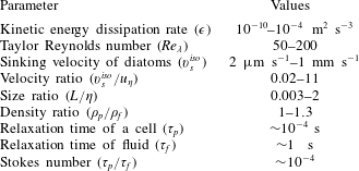
A summary of the parameter values relevant to marine diatoms. The value of
 $\unicode[STIX]{x1D716}$
is considered
 $10^{-6}$
 $~\text{m}^{2}~\text{s}^{-3}$
for calculating
 $\unicode[STIX]{x1D70F}_{f}$
and
 $Re_{\unicode[STIX]{x1D706}}$
.
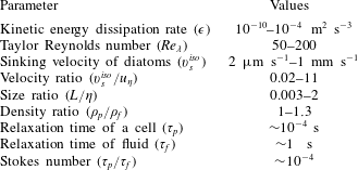
Characteristic velocities at dissipation scale in the ocean (
 $u_{\unicode[STIX]{x1D702}}=(\unicode[STIX]{x1D708}\unicode[STIX]{x1D716})^{1/4}$
) are on the order of
 $0.01$
–
 $0.1~\text{mm}~\text{s}^{-1}$
, resulting in a velocity ratio
 $v_{s}^{iso}/u_{\unicode[STIX]{x1D702}}\approx 1{-}4$
(assuming maximum
 $v_{s}^{iso}$
of
 $1~\text{mm}~\text{s}^{-1}$
). Densities of marine diatoms
 $\unicode[STIX]{x1D70C}_{p}$
have not been measured directly but estimated from the Stokes equation for settling spheres, based on measured sinking velocities. Densities were found to be in the range
 $1.03$
–
 $1.15~\text{g}~\text{cm}^{-3}$
for actively growing cells with higher values for cells in senescence (
 $1.059$
–
 $1.33~g~cm^{-3}$
; Eppley et al.
Reference Eppley, Holmes and Strickland1967). Average density of surface seawater
 $\unicode[STIX]{x1D70C}_{f}$
is
 $1.025~\text{g}~\text{cm}^{-3}$
and thus the density ratio relevant to the parameter space of phytoplankton is in the range 1–1.3. Table 2 summarizes the parameter values relevant to marine diatoms.