





1. Introduction
The solar wind is the supersonic flow of coronal plasma out through the interplanetary medium (Parker Reference Parker1958). It is primarily made up of protons, electrons, and alpha particles, alongside trace heavy ions such as oxygen, carbon, and iron. The evolution of the solar wind through the inner heliosphere is driven by the global magnetic field, the heating and acceleration processes at work in-situ as the wind expands, and the non-linear interactions (turbulence) taking place in this collisionless medium. This evolution is a complex process that requires a combination of theory, modeling, and multi-spacecraft in-situ and remote measurements to probe. It has implications for our ability to accurately model the evolution of the wind, and thus correctly understand the space weather impacts. While the expansion and evolution of the wind can be studied in-situ, identifying its source requires additional work. We must use a combination of modeling, remote measurements, and in-situ tracers of source region to connect the expanding solar wind to the magnetic topological region of emergence.
Understanding the dynamics and structure of the magnetic field at the source of the solar wind is one of the primary science goals for the Parker Solar Probe (PSP; Fox et al. Reference Fox, Velli, Bale, Decker, Driesman, Howard, Kasper, Kinnison, Kusterer, Lario, Lockwood, McComas, Raouafi and Szabo2016) mission. This is often done with magnetic connectivity methods, whereby models of the global magnetic field are produced and spacecraft trajectories and flown through these models to then trace the in-situ observations along modeled field lines down to their source (e.g. Badman et al. Reference Badman, Bale, Martínez Oliveros, Panasenco, Velli, Stansby, Buitrago-Casas, Réville, Bonnell, Case, Dudok de Wit, Goetz, Harvey, Kasper, Korreck, Larson, Livi, MacDowall, Malaspina, Pulupa, Stevens and Whittlesey2020). This provides an estimation of the ‘footpoints’ for the emerging solar wind for further study. These estimates of solar source region can be coupled with heavy ion diagnostics, which also relate to the solar source and are conserved through radial evolution, to trace the source (and acceleration) mechanism(s) associated with the solar wind.
Various works have identified the source of the fast solar wind (FSW; where
 $V_{sw} \geq 500$
km/s at 1 AU) to be coronal hole (CH) structures (McComas et al. Reference McComas, Riley, Gosling, Balogh and Forsyth1998, Reference McComas, Ebert, Elliott, Goldstein, Gosling, Schwadron and Skoug2008). From a magnetic topology perspective, these are regions of open fields lines (which we note is a necessity for the emergence of the solar wind), and from an observational perspective, CH structures are cool, low density regions with low magnetic field strength that manifest as dark regions in EUV observations. In contrast, there are streamer and active region (AR) structures that are associated with strong magnetic fields at the photosphere, and bright loop structures in EUV. In addition to the fast and slow (
 $V_{sw} \leq 500$
km/s) classification scheme for the solar wind, recent work has shown the need to include turbulence parameters such as cross helicity (
 $\sigma_C$
; which describes the degree of correlation between velocity and magnetic field fluctuations) in wind categorization (D’Amicis and Bruno Reference D’Amicis and Bruno2015). Using this parameter produces a class of wind known as slow Alfvénic solar wind (SASW) which has low speeds, and high cross helicity (highly Alfvénic), in contrast to the classical (non-Alfvénic) slow wind which has low speeds and low cross helicity.
The slow Alfvénic wind show plasma parameters that are similar to fast wind streams, despite having slower speeds (e.g. D’Amicis and Bruno Reference D’Amicis and Bruno2015). This similarly in in-situ observations, especially composition ratios, has been tied to the idea that SASW may emerge from similar source regions to the FSW. We outline methodology for estimating the connectivity of the solar wind and its source and discuss the use of composition metrics (measurements of heavy ion abundances and charge states) as a tracer of solar wind source region. We show that the majority of SASW observed by PSP seems to emerge from coronal holes and their boundaries, but that there may exist a second class of SASW whose source lies closer to that of the classical non-Alfvénic slow wind. To close the gap in our understanding of solar wind connectivity requires multi-spacecraft measurements of the solar magnetic field, alongside measurements of coronal diagnostics (e.g. coronal densities, temperatures, outflow speeds, and heavy ion composition) to connect the wind to its source.
2. Methods for Estimating Magnetic Connectivity
To connect observations of the solar wind in-situ with its source, requires a model (or extrapolation) of the global magnetic field from the photosphere, out to the spacecraft’s heliocentric distance. There are various methods employed in magnetic connectivity science, with varying degrees of complexity in the methodology for extrapolating the photospheric magnetic field.
2.1. Modeling Inputs
All models require an input lower boundary condition, a measurement of the photospheric magnetic field, which is typically taken from the ground-based Global Oscillation and Network Group (GONG; Harvey et al. Reference Harvey, Hill, Hubbard, Kennedy, Leibacher, Pintar, Gilman, Noyes, Title, Toomre, Ulrich, Bhatnagar, Kennewell, Marquette, Patron, Saa and Yasukawa1996) or the space-based Helioseismic and Magnetic Imager (HMI; Scherrer et al. Reference Scherrer, Schou, Bush, Kosovichev, Bogart, Hoeksema, Liu, Duvall, Zhao, Title, Schrijver, Tarbell and Tomczyk2012) aboard the Solar Dynamics Observatory (SDO; Pesnell et al. Reference Pesnell, Thompson and Chamberlin2012). These measurements provide a synchronic (single point in time) measurement of the photospheric field which can then be extrapolated with a model of your choosing. However, these synchronic measurements only provide a measurement of the Earth-facing hemisphere of the solar photosphere. Modeling the global magnetic field requires an input of the full Sun, these are often known as Carrington or synoptic maps. Full-Sun photospheric magnetic field maps are typically produced one of two ways: by combining a Carrington rotation’s worth of observations of the photospheric field with some merging technique and accounting for line-of-sight effects, or via evolution of the observed magnetic flux to the part of the disk that is not observed. This method is known as flux transport, and models such as the Air Force Data Assimilative Photospheric Flux Transport (ADAPT; Arge et al. 2010) provide well tested pathways to do this.
2.2. Connectivity via Potential Field Extrapolations
The simplest method for extrapolation of the photospheric magnetic field is known as the Potential Field Source Surface (PFSS; Altschuler and Newkirk Reference Altschuler and Newkirk1969) model. It requires two user inputs as boundary conditions: the photospheric magnetic field and a source surface height (
 $R_{ss}$
) where the magnetic field is considered purely radial. Between these two points, the model assumes a magnetostatic or current-free (
 $\nabla \times \mathbf{B} = 0$
) corona, and represents the magnetic field as a gradient of a scalar potential (
 $\mathbf{B} = - \nabla \psi$
). As
 $\nabla \cdot \mathbf{B} = 0$
, we can write
 \begin{equation} \nabla \cdot \mathbf{B} = \nabla \cdot ( - \nabla \psi) = \nabla^2 \psi = 0\end{equation}
giving Laplace’s equation (Equation 1). A solution can then be determined with the two boundary conditions described above. This can be solved in spherical coordinates to provide an estimated extrapolation of the global magnetic field out to the source surface (
 $R_{ss}$
).
To connect spacecraft observations to the extrapolated magnetic field, requires other assumptions about the propagation of the solar wind beyond the source surface. The simplest method is to ballistically propagate the spacecraft trajectory at its (variable) heliocentric distance (
 $R_{sc}$
) down to the source surface height. This method assumes that any point in the heliosphere can be propagated inwards by assuming propagation along a Parker spiral line, with some set speed (Nolte and Roelof Reference Nolte and Roelof1973). While the real solar wind is accelerating as it expands, the errors associated with the constant speed assumption has been shown to be
 $\leq 10^\circ$
(Nolte and Roelof Reference Nolte and Roelof1973; Badman et al. Reference Badman, Bale, Martínez Oliveros, Panasenco, Velli, Stansby, Buitrago-Casas, Réville, Bonnell, Case, Dudok de Wit, Goetz, Harvey, Kasper, Korreck, Larson, Livi, MacDowall, Malaspina, Pulupa, Stevens and Whittlesey2020; Ervin et al. 2024c). With this ballistic propagation, the spacecraft trajectory is now connected to the model of the magnetic field. All that is left is to trace along modeled field lines to estimate the spacecraft’s connectivity to the photosphere. It is important to note that this method can only trace along field lines that are topologically ‘open’ at the source surface, meaning that we can never show connection to topologically ‘closed’ structures that may open at larger heights in the corona.
This PFSS + ballistic propagation method is an incredibly computationally efficient, and easily usable method for providing an estimation of the magnetic connectivity of in-situ observations to their source. Despite its usability, the PFSS and ballistic propagation combination includes a variety of user introduced, and general sources of error. The choice of which input magnetogram to use (what data source, what observation time, how to extrapolate to the far-side of the Sun), which source surface height, and which speed for the ballistic propagation can lead to uncertainties on the order of 10s of degrees in the modeled footpoints. The choice of PFSS boundary conditions can be optimized by comparing the modeled heliospheric current sheet with the observed crossing of the neutral line, or by comparing the modeled magnetic field strength with what is observed in-situ (Badman et al. Reference Badman, Bale, Martínez Oliveros, Panasenco, Velli, Stansby, Buitrago-Casas, Réville, Bonnell, Case, Dudok de Wit, Goetz, Harvey, Kasper, Korreck, Larson, Livi, MacDowall, Malaspina, Pulupa, Stevens and Whittlesey2020; Ervin et al. 2024c). In addition, the assumptions that go into the model itself are not physically accurate, and the steady-state nature of these models is not able to capture the time-dependent nature of magnetic connectivity in the heliosphere. Despite this, with rigorous uncertainty estimation and the understanding that these are estimates of the spacecraft connectivity, PFSS models provide an incredible tool for understanding the solar wind’s varied sources.
2.3. Connectivity via Magnetohydrodynamic Simulations
While the PFSS model provides a computationally efficient method for extrapolating the global field, it makes nonphysical assumptions about the potential nature of the magnetic field in the lower corona. More physically complex methods to extrapolate the magnetic field exist, and a commonly used method is magnetohydrodynamic (MHD) modeling. These models take an equivalent inner boundary condition as potential field models, a full-Sun map of the photospheric magnetic field. The model then integrates the MHD equations (with varied assumptions and in varied forms) to provide a description of the plasma and magnetic fields. Different models use varied assumptions (e.g. different heating terms) for driving the supersonic solar wind, and provide a method through which coronal heating can be studied.
There are a variety of state-of-the-art codes to extrapolate the photospheric magnetic field by integrating the MHD equations with some set of assumptions. In our work, we use the Predictive Science Inc. (PSI) MHD algorithm outside a Sphere (MAS) code to solve the MHD equations on a nonuniform mesh grid (Riley et al. Reference Riley, Lionello, Caplan, Downs, Linker, Badman and Stevens2021). This code has been shown to well replicate remote and in-situ observations that can be derived from the model. Synthetic observables can be produced to qualitatively study how well the model does at replicating the observed magnetic field and density structure in the observed corona. One can fly a spacecraft through the modeled field to produce a timeseries of modeled in-situ observations, which can then be directly compared to spacecraft measurements. In contrast to the potential field extrapolation, MAS can model the magnetic field throughout the inner heliosphere, and thus ballistic propagation is not necessary for estimating spacecraft connectivity. We show an example comparing the outputs of PFSS and MAS simulations with in-situ measurements of polarity in Figure 1. We note that the PFSS and MAS extrapolations produce similar current sheets. This Figure shows how a comparison of modeled and measured magnetic field polarities can be used a method of model validation, and for inter-model comparison.
Figure from Ervin et al. (Reference Ervin, Bale, Badman, Bowen, Riley, Paulson, Rivera, Romeo, Sioulas, Larson, Verniero, Dewey and Huang2024a) showing a comparison of model outputs between PFSS and MHD (PSI/MAS) magnetic field extrapolations compared with in-situ measurements from Parker Solar Probe and Solar Orbiter. Panel (a) shows the magnetic field polarity as a function of source surface (2.5
 $\mathrm{R}_\odot$
) longitude. The modeled polarities are pulled directly from the PFSS and MHD coronal field extrapolations. The Parker and Orbiter polarities are projected down from the spacecraft trajectory to 2.5
 $\mathrm{R}_\odot$
using ballistic propagation as described in Section 2.2. Panel (b) shows the modeled current sheets from the PFSS (dotted) and MHD (solid) simulations. The background is the global magnetic field at 2.5
 $\mathrm{R}_\odot$
from the MHD simulation. The projected Parker Solar Probe trajectory is overlaid and colored by the measured polarity at the spacecraft.

Figure 1 Long description
Panel A: A bar graph shows magnetic field polarity as a function of source surface longitude. The x-axis represents source surface longitude in degrees, ranging from 0 to 360 degrees. The y-axis lists different models and measurements: PFSS, MHD, Parker, and Orbiter. The bars are color-coded to indicate polarity, with blue representing negative polarity and red representing positive polarity. Panel B: A contour plot displays modeled current sheets from PFSS (dotted lines) and MHD (solid lines) simulations. The background is a color map of the global magnetic field at 2.5 solar radii from the MHD simulation, with colors ranging from blue (negative) to red (positive). The x-axis represents Carrington longitude in degrees, and the y-axis represents Carrington latitude in degrees. The projected Parker Solar Probe trajectory is overlaid and colored by the measured polarity at the spacecraft.
2.4. Accessing source region parameters
Estimation of the footpoint location for where in-situ measurements of the solar wind emerged from allows us to study characteristics associated with the source. To do this, we utilize remote observations of the photosphere and corona, specifically magnetograph and EUV observations. We extract values of the remote observations at the pixel coordinate associated with the location of the estimated footpoint. We can do this for each point in our in-situ timeseries where we have an estimated source region location (see Ervin et al. (Reference Ervin, Bale, Badman, Rivera, Romeo, Huang, Riley, Bowen, Lepri and Dewey2024b)). This allows us to produce a ‘timeseries’ of source region parameters. We do this for measurements of the photospheric field, which allows us to understand the magnetic field strength at the solar wind’s estimated source, and differentiate between weak and strong photospheric fields. The same method is used for EUV observations from the Atmospheric Imaging Assembly (AIA; Lemen et al. 2012) on the SDO, giving insight into the temperature and density of the plasma in the corona.
We also look at the magnetic expansion factor (
 $f_s$
) in the same way. This provides a measure of how over-expanded the magnetic field is, relative to purely
 $1/r^2$
spherical expansion, between the photosphere (
 $R_0, \lambda_0, \phi_0$
) and a second point (
 $R_1, \lambda_1, \phi_1$
).
 \begin{equation} f_{s} = \left( \frac{R_0}{R_1} \right)^2 \frac{B_R{R_0, \lambda_0, \phi_0}}{B_R{R_1, \lambda_1, \phi_1}}\end{equation}
This can be done between the photosphere and the source surface (
 $f_{ss}$
) or between the photosphere and the spacecraft location. A large body of work exists that has studied the relation between solar wind speed and expansion factor (e.g. Wang and Sheeley Reference Wang and Sheeley1990). In general, it has been found that slower wind emerges from regions with larger expansion factors. A more rapidly diverging field (larger expansion) has a higher critical point (where the wind becomes supersonic) and thus more heating would occur prior to the transition of the wind from subsonic to supersonic. Heating above the critical point causes the wind speed to increase (Leer and Holzer Reference Leer and Holzer1980), and thus slower wind from rapidly expanding fields follows this relation. However, not all slow wind is associated with large expansion factors, and there may be an additional dependence on Alfvénicity in addition to just wind speed.
3. Compositional Diagnostics
While magnetic field modeling provides a method through which we can estimate connectivity to topological structures in the coronal field, the uncertainties in our models are such that another connectivity tool is vital for the full picture. Compositional diagnostics provide another lens through which connectivity can be probed. Measurements of heavy ion charge state ratios (e.g.
 $\mathrm{O}^{7+} / \mathrm{O}^{6+}$
) and total elemental abundance ratios (Fe/O) can be related to the topology of the structure from which the solar wind emerged (Rivera et al. Reference Rivera, Higginson, Lepri, Viall, Alterman, Landi, Spitzer, Raines, Cranmer, Laming, Mason, Wallace, Raymond, Lynch, Gilly, Chen and Dewey2022). These ratios often stay approximately conserved throughout radial evolution, and thus make for a compelling tracer of solar source.
3.1. Heavy Ion Ratios
Heavy ion ratios allow us to probe the ionization level of the solar wind plasma. The processes that ionize the solar wind occur low down in the corona as ionization and recombination rates are dependent upon (and proportional to) the electron density (Owocki et al. Reference Owocki, Holzer and Hundhausen1983). As the wind radially expands, there is a dramatic drop in the electron density to a point where the density is too low for ionization and recombination processes to occur. Known as the freeze-in point, after this radial distance (typically 1-2
 $R_\odot$
depending on the ion), ionization ratios are frozen-in and undergo little radial evolution (Hundhausen Reference Hundhausen1968). Therefore, in-situ measurements of heavy ion ratios can serve as a proxy for the electron properties at the source. Various works have shown the relation of low charge state ratios with wind emerging from CH structures (von Steiger and Zurbuchen Reference von Steiger and Zurbuchen2011), while higher charge states have been related to CH boundaries (Antiochos et al. Reference Antiochos, Linker, Lionello, Mikić, Titov and Zurbuchen2012), helmet streamers (Zhao et al. Reference Zhao, Zurbuchen and Fisk2009; Zhao and Fisk Reference Zhao and Fisk2011; Zhao et al. Reference Zhao, Landi, Zurbuchen, Fisk and Lepri2014), and active regions (Liewer et al. Reference Liewer, Neugebauer and Zurbuchen2003).
3.2. Elemental Composition
Total elemental composition, specifically ratios between elements, allow us to probe the effects of the first ionization potential (FIP) bias, where abundances of low-FIP elements are enhanced over high-FIP elements. There are various ratios that can be studied to probe this fractionation, the most common of which is Fe/O. Spectroscopic measurements of coronal loops have shown a correlation between FIP bias and loop lifetime, e.g. the longer the loop exists, the larger the Fe/O ratio (Feldman and Marsch Reference Feldman and Marsch1997). Theoretical work by (Laming Reference Laming2015; Laming Reference Laming2017; Laming et al. Reference Laming, Vourlidas, Korendyke, Chua, Cranmer, Ko, Kuroda, Provornikova, Raymond, Raouafi, Strachan, Tun-Beltran, Weberg and Wood2019) has tied the enhancement of low-FIP elements in coronal loops to the generation of the ponderomotive force in the upper chromosphere. As this force is only felt by ions, it will lead to an enhancement in ions over neutrals, leading to elemental fractionation in the upper solar atmosphere. Therefore, plasma that quickly flows out of the lower solar atmosphere along open field lines should show low FIP bias in comparison to plasma that spent time within coronal loops. One can study the in-situ FIP bias by comparing measurements of elemental abundance ratios, to their photospheric values determined from remote spectroscopic observations (e.g.
 $\mathrm{(Fe/O)} / \mathrm{(Fe/O)}_\mathrm{phot})$
. A larger ratio indicates more FIP enhancement (canonically tied to more time spent in coronal loops).
4. Discussion
4.1. Combining coronal modeling and in-situ metrics of elemental composition
We study a Parker spiral alignment between PSP and Solar Orbiter to leverage the advantages of both spacecraft in understanding the connectivity of observed streams. We look at two FSW streams and one SASW stream and compare with near-HCS wind. Streams are identified as Alfvénic (or non-Alfvénic) using the cross helicity measured at PSP, and as fast or slow using the in-situ wind speed at Solar Orbiter (as we expect the solar wind to have reached its asymptotic wind speed at Solar Orbiter distances, as opposed to PSP distances). We use PFSS and MHD simulations to trace the measured solar wind streams to their estimated source and extract source region properties. We compare the modeled sources with the compositional diagnostics measured in-situ by the Solar Orbiter (Müller, D. et al. 2020) Heavy Ion Sensor (HIS; Livi et al. Reference Livi, Lepri, Raines, Dewey, Galvin, Louarn, Collier, Allegrini, Alterman, Bert, Bruno, Chornay, D’Amicis, Eddy, Ellis, Fauchon-Jones, Fedorov, Gershkovich, Holmes, Horbury, Kistler, Kucharek, Lugaz, Nieves-Chinchilla, O’Brien, Ogasawara, Owen, Phillips, Ploof, Rivera, Spitzer, Stubbs and Wurz2023) to understand the relation between compositional metrics and solar source. Figure 2 shows the estimated footpoints from our modeling methods and a Table 1 provides a summary of values that we determined during this study.
Footpoints estimated from our magnetic connectivity methods over plotted on EUV observations of the sources associated with the wind streams studied in Ervin et al. (Reference Ervin, Bale, Badman, Rivera, Romeo, Huang, Riley, Bowen, Lepri and Dewey2024b). The EUV images are AIA observations from the estimated time of emergence of these streams. Panels (a), (b), and (c) show the estimated footpoints for the FSW (1), FSW (2), and SASW streams discussed in Table 1. Figure from Ervin et al. (Reference Ervin, Bale, Badman, Rivera, Romeo, Huang, Riley, Bowen, Lepri and Dewey2024b).

A summary of values associated with the wind streams examined by Ervin et al. (Reference Ervin, Bale, Badman, Rivera, Romeo, Huang, Riley, Bowen, Lepri and Dewey2024b). Two fast solar wind (FSW) streams with high Alfvénicity, one slow Alfvénic solar wind (SASW) stream, and one stream at the HCS were looked at.

Table 1 Long description
A table comparing wind stream properties and modeled sources. The table has five rows and eight columns. Column headers are Wind Stream, Modeled Source, f sub a, B sub 0, O 7+/O 6+, C 6+/C 4+, and (Fe/O)/(Fe/O) sub phot. Row 1: FSW (1), Equatorial CH, greater than or equal to 2, approximately 1 G, approximately 0.06, greater than or equal to 2, 1 to 2.5. Row 2: FSW (2), CH Boundary, approximately 100, less than or equal to 25 G, approximately 0.06, less than or equal to 1, 1 to 2.5. Row 3: SASW, CH Boundary, approximately -12, less than or equal to 15 G, 0.03 to 0.35, 1.5 to 9, 1 to 5.5. Row 4: HCS, Current Sheet, N/A, N/A, 0.25 to 0.35, 6 to 12, 3 to 4.
*We note that this stream was near the current sheet, leading to the large expansion factor.
We find that the highly Alfvénic streams emerge from equatorial CHs and their boundaries, and that the SASW stream emerges from a highly overexpanded CH boundary in comparison to the under-expanded sources of the FSW streams. The SASW shows a large variance in charge state and elemental composition. This could indicate mixing of plasma between open and closed field structures due to interchange reconnection driving the emergence of the slow wind (consistent with FIP bias ideas proposed by Laming (Reference Laming2017)). However, work such as Réville et al. (Reference Réville, Rouillard, Velli, Verdini, Buchlin, Lavarra and Poirier2021) has shown the ability for FIP-biased plasma to be produced in CHs (and not just coronal loops) provided that turbulence is the dominant driver of coronal heating and solar wind acceleration. Solar Orbiter observations of heavy ion diagnostics coupled with modeling of solar source could differentiate between proposed mechanisms from ponderomotive force generation and the FIP effect.
4.2. Understanding source region characteristics
The above study focused on a specific interval of Alfvénic wind streams, and we were interested in expanding this work to understand what the source region characteristics look like for streams on a more statistical basis. Ervin et al. (2024c) looked at the in-situ and source region characteristics of slow Alfvénic solar wind streams observed by PSP. Using a heliocentric distance based classification scheme to account for solar wind acceleration, we identified streams as fast or slow and then Alfvénic (
 $|\sigma_C| \geq 0.7$
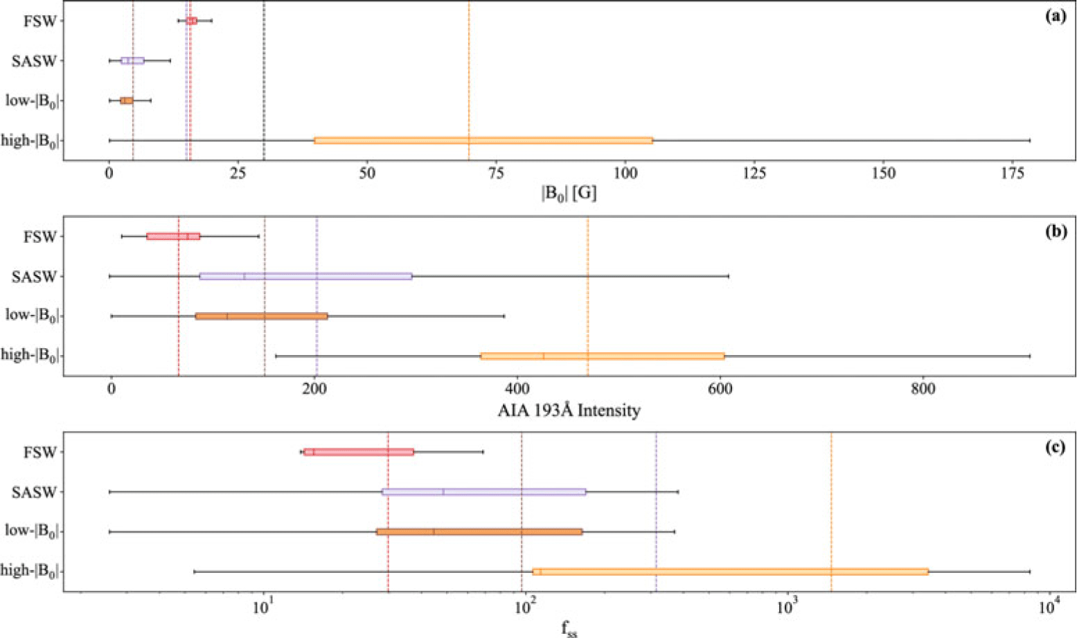
) or non-Alfvénic. We then looked at the in-situ characteristics of these streams, such as the alpha particle abundance, and the source region characteristics (calculated via the methods described in Section 2.4). Figure 3 shows a comparison of source region parameters associated with FSW and SASW streams studied in Ervin et al. (2024c).
Overview of source region parameters extracted from remote observations at the footpoints of the wind streams estimated from PFSS modeling. We show these parameters for the FSW, SASW, and the low-
 $\mathrm{B}_0$
and high-
 $\mathrm{B}_{0}$
SASW subcategories. The box plot shows the inner quartile range (25%-75%) percentile and the solid line shows the median value. The dashed vertical lines show the mean of each parameter for the type of wind stream. Figure from Ervin et al. (2024c).

Figure 3 Long description
Panel A: A box plot compares the magnetic field strength (|B0| in Gauss) for different types of solar wind: FSW, SASW, low-|B0|, and high-|B0|. The inner quartile range (25%-75%) is shown, with the median value indicated by a solid line and the mean by dashed vertical lines. Panel B: Another box plot shows AIA 193 Angstrom intensity for the same types of solar wind, with similar markers for quartile range, median, and mean. Panel C: A third box plot depicts the cross helicity (f_ss) for the different solar wind types, again with markers for quartile range, median, and mean.
Through our modeling, we identified two sub-classes of SASW. One which emerged from source regions with low footpoint field strength (low-
 $\mathrm{B}_{0}$
) and another from high-
 $\mathrm{B}_{0}$
regions. We then investigated the in-situ and source region characteristics of these two classes. We tied the low-
 $\mathrm{B}_{0}$
streams to emergence from overexpanded CHs/CH boundary structures and note that these high-
 $\mathrm{B}_{0}$
streams warrant further investigation. Through this analysis we found:
-
(1) Distinct in-situ signatures of fast, slow, and slow Alfvénic solar wind
-
(a) Large variance in alpha particle composition indicating that more work is required to understand the processes leading to alpha particle signatures and how differential streaming impacts this
-
-
(2) Two populations of SASW based on source region and in-situ characteristics
-
(a) CH-like/CH boundary structures: high expansion factor + low mass flux + low intensity = large heating below critical point in a cooler structure (slow wind from CH-like region)
-
(b) Non-CH structures: high expansion factor + high mass flux + high intensity = large heating below critical point in a hotter structure (slow wind from non-CH region). We note that these streams should be studied in more detail and additional work is necessary to understand
-
We note that heavy ion diagnostics could help close our understanding on the source region of these low footpoint field strength SASW streams. Measurements of heavy ion ratios and elemental composition could help point to whether this wind spent time in coronal loop structures prior to emergence. Pagel et al. (Reference Pagel, Crooker, Zurbuchen and Gosling2004) has shown correlation of the proton specific entropy and oxygen charge state ratio, indicating the potential of using specific entropy as a high cadence proxy for
 $\mathrm{O}^{7+} / \mathrm{O}^{6+}$
and perhaps a tracer of solar wind source. Additional work looking at this correlation closer to the Sun is vital to complete our understanding of charge state proxies, and how entropy relates to source and solar wind expansion.
5. Summary and Future Prospects
Through a combination of in-situ metrics and magnetic field models, we study the source regions and characteristics associated with slow Alfvénic solar wind (SASW) streams in the inner heliosphere. Our work indicates that the majority of SASW streams emerge from the (often over-expanded) boundaries of open field structures, with a small subset that seem to emerge from high field strength regions warranting further investigation. We see large variance in the alpha particle composition (sometimes used as a tracer of solar wind source) for these streams, and note that additional work is required to understand the processes leading to alpha particle composition signatures, and how the
 $N_\alpha / N_p$
ratio evolves through the inner heliosphere due to differential streaming between protons and alpha particles.
Understanding the connectivity and source regions of solar wind flows directly relates to our ability to understand the wind’s in-situ properties, and thus accurately forecast stream evolution through the inner heliosphere. Connecting in-situ measurements with their source requires an accurate picture of the global magnetic field in a time-dependent manner. While steady state models allow us to estimate connectivity for ambient wind streams, they do not account for changes in magnetic topology associated with transient events (Downs et al. Reference Downs, Linker, Caplan, Mason, Riley, Davidson, Reyes, Palmerio, Lionello, Turtle, Ben-Nun, Stulajter, Titov, Török, Upton, Attie, Jha, Arge, Henney, Valori, Strecker, Calchetti, Germerott, Hirzberger, Suárez, Rodríguez, Solanki, Cheng and Wu2025). Time-dependent models are necessary to fully capture the ever changing complexity of the solar magnetic field due to interactions between streams, and with transient events. Improvements in remote observations of the photospheric field are also necessary, requiring global coverage for the production of proper input boundary conditions to our models.
Estimation of uncertainties associated with these coronal magnetic field models and improvement in methodology for model validation is also necessary. In-situ and remote heavy ion diagnostics provide a path forward. These diagnostics can connect in-situ measurements with their source, and there exists very limited coverage of these measurements. These validation efforts will directly improve our modeling and forecasting capabilities, alongside our understanding of the fundamental physical mechanisms at work in the lower solar atmosphere.
6. Acknowledgments
TE thanks the IAU Travel Grant and the AAS/SPD Metcalf Award for supporting attendance of the IAU Symposium 400: Solar and Stellar Multi-Scale Activity. TE acknowledges funding from The Chuck Lorre Family Foundation Big Bang Theory Graduate Fellowship, NASA contract NNN06AA01C and grant 80NSSC20K1285.

 R⊙
 R⊙
 R⊙


 B0
 B0

 Open access

