


1. Introduction
In practice, failures of systems are often preceded by some defects that can evolve into the final failures or be eliminated. For instance, in engineering, fatal failures of structures or systems occur after some time has elapsed from the initiating defect. However, this can be prevented by the timely repair. In medicine, the onset of a disease (e.g., seroconversion of HIV) happens at some point in time, which eventually results either in the diagnosed condition (e.g., AIDS) or even in a death of a patient if not treated properly. In finance, some triggering events can eventually lead to a default of a financial institution or some other important dysfunction if not properly and timely addressed. Thus, there is usually some latent period of time when the initial defect develops into the fatal event [Reference Cha and Finkelstein7].
Thus, for repairable systems, a defect, if repaired within a specified time period, does not necessarily develop into a fatal failure (FF) due to some inertia that keeps, for example, the output characteristics of a system within tolerable limits [Reference Goyal, Finkelstein and Hazra15]. For instance,
• If repair of the failed navigational equipment of the marine navigation system is performed within a relatively short time, then the latitude and longitude of a vessel remain approximately the same and therefore, the initial defect does not become the FF. Therefore, we see a certain inertia in these output characteristics. Obviously, it does not apply to the heading; thus, the described property is output-specific in this example.
• In some power generation systems, a defect or failure is classified as catastrophic only if it remains unresolved beyond a specified time frame. For example, in a power station comprising multiple generating units, the continuity of electricity supply can still be considered as acceptable during the repair of one or more generating units, provided the duration of repair does not exceed a predetermined threshold value.
Other situations when a timely repaired defect or failure does not result in the FF are (but not limited to): thermo-stabilization systems that usually have a remarkable inertia of the described type; pumping systems with intermediate storage, communication and weather satellites, unmanned aerial vehicles, military missions, medical equipment malfunction, etc.
On the other hand, at least in some of the provided examples, the described inertia after the occurrence of a defect is decreasing with each successfully repaired defect. This can be interpreted in terms of the corresponding imperfect repair that technically restores a system to a functional state but is not perfectly restoring the inertia capabilities of a system (see, e.g., [Reference Cheng and Zhao6,Reference Cha and Finkelstein7,Reference Kurt and Kharoufeh18,Reference Li and Kagaris21]). However, our models admit a broader interpretation. They can also represent the loss of physical buffering capacity (e.g., due to thermal or mechanical inertia), reduction of safety margins caused by cumulative damage, increasing response times in human or organizational systems, or logistical constraints leading to progressively longer repairs. Therefore, the framework developed in this paper can be viewed more generally as describing systems with diminishing tolerance to defects over time, irrespective of the specific physical or operational origin of this effect.
We will consider two new important models that describe these effects and have, in our opinion, theoretical and practical value.
Model 1. The distribution of time of repair is fixed, but after each repair, the deterministic period of inertia  ${\delta _i},{\text{ }}i = 1,2,$ is decreasing, that is,
 ${\delta _1} \gt {\delta _2},\,\, \gt {\delta _3} \cdots $
Model 2. The baseline  $\delta $ is fixed; however, the time of repair is stochastically increasing with each repaired defect.
For both models, we will also consider a practically important case with a limited number of repairs [Reference Kurt and Kharoufeh18]. For instance, consider aircraft engine turbine blades, which endure high temperatures and centrifugal stresses, resulting in elongated microstructure particles. This elongation diminishes fatigue strength, leading to the formation of voids and cracks at the blade tips. These blades can undergo rework only a limited number of times before replacement to ensure flight safety. Thus, every repair decreases the ability of a system to perform its mission, however, within the tolerable limits. When these limits are “depleted” the FF occurs. Another, probably more common reason for this restriction is just the limited number of the spare parts needed for repair [Reference Asadi1,Reference Goyal, Finkelstein and Hazra15].
Due to the “renewal nature” of the considered models [Reference Barlow and Proschan3], we obtain survival probabilities of interest by deriving and analyzing the corresponding integral equations of the Volterra type that can be effectively solved via the Laplace transform (LT).
In our paper, we use the term time redundancy to describe the delay-tolerance mechanism, highlighting the presence of a temporal buffer (or inertia) that prevents immediate failure. It was used in earlier work (e.g., [Reference Gnedenko, Belyaev and Solovjev4,Reference Goyal, Finkelstein and Hazra15,Reference Zarunij27]) and provides an intuitive interpretation of the underlying mechanism. This “buffer” is not necessarily linked to repair, which is just an important but specific interpretation. Our recent paper [Reference Goyal, Finkelstein and Hazra15] considers the time redundancy problem with additional constraints, that is, the FF also occurs when the next defect after the completion of repair of the previous one is too close. However, the baseline  $\delta $ and the distribution of the repair time are fixed in this paper. Note that, Section 2 is, in fact, a specific case of the model considered in paper [Reference Goyal, Finkelstein and Hazra15], but obtained in a different, meaningful way via the integral equations (see also paper [Reference Vaurio25]). For repairable systems, the somewhat close (but not the same) concept of tolerable delay has been considered for availability analysis, optimal spare allocation, etc. For instance, Bao and Cui [Reference Bao and Cui2] have proposed a model for evaluating the availability of repairable systems based on Markov processes, wherein failures can either be neglected or delayed based on repair time (see also papers [Reference Qiu and Cui17,Reference Levitin, Xing and Dai19,Reference Zhou and Wang28]). Cha and Finkelstein [Reference Cha and Finkelstein8] considered a delay when initial defects were developing into the FF. Park et al. [Reference Park, Jung and Park23,Reference Park, Jung and Park24] have described maintenance models for repairable systems under a renewable warranty policy, where systems are either minimally repaired or replaced if a repair cannot be completed within a certain time. Dreyfuss and Giat [Reference Dreyfuss and Giat5] discussed the optimization of spare items allocation in multilocation repair system by considering tolerable delay in service. It should be noted that the considered settings, in the current paper, resemble in a way some delta-shock models when a system operating in a shocks environment fails if the time between the two consecutive shocks is less than the prefixed threshold
 $\delta $. These models were extensively studied in the literature (see, e.g., [Reference Eryilmaz9–Reference Goyal, Hazra and Finkelstein14,Reference Li and Zhao20,Reference Lyu, Qu, Yang, Ma, Lu and Pecht22,Reference Wang and Peng26], to name a few).
The paper is organized as follows. In Section 2, along with some preliminary considerations, the basic approach for the fixed threshold based on renewal equations is described and illustrated. In Sections 3 and 4, the survival probabilities are derived for Models 1 and 2, respectively. Section 5 considers the case with a limited number of repairs for both models, while Section 6 presents some conclusions. Some examples and illustrations for the case of the exponential distributions of times to a defect and of repair are given throughout the paper.
2. Basic setting and preliminaries
A system starts operating at  $t=0$. The times to the first and subsequent defects, Xi, i = 1, 2, … and the repair times
 ${Y_i},i = 1,2, \ldots $ after each defect are i.i.d. with the cumulative density functions (c.d.f.s)
 $F( t ),{\text{ }}G( t ),$ probability density functions (p.d.f.s)
 $f( t ),{\text{ }}g( t ){\text{ }}$and survival functions
 $\bar F( t )$ and
 $\bar G( t )$, respectively. They will be referred to as X and Y, where applicable. All random variables
 ${X_i}{\text{ }}$ and
 ${Y_i}$ are independent f each other. If the time of the ith repair, i = 1, 2, 3,… becomes larger than the threshold
 ${\delta _i}{\text{ }}$, for the first time, then the final failure (FF) occurs. We assume that the thresholds are decreasing with i as
 ${\delta _1} \gt {\delta _2}$, >
 ${\delta _3}$…. showing a certain deterioration that can also be interpreted as the corresponding imperfect repairs. This setting will be considered in the next section (Model 1), whereas in Section 4, we assume that the threshold is fixed while the repair times are stochastically increasing with each repaired defect (Model 2). We denote by T the time to the FF for both models and their c.d.f. and p.d.f. by
 ${\text{ }}{F_f}( t ) = \Pr \left( {T \leq t} \right){\text{ and }}{f_f}( t )$, respectively. We are interested in obtaining the corresponding survival probabilities
 $S( t ) = {\text{Pr}}(T \gt t)$ for both models.
In this introductory and in a way supplementary section, we describe the setting and obtain  $S( t )$ for the simplified model when there is still no deterioration in the threshold or in the repair time. This can also be considered, as a specific case of our paper: Goyal et al. [Reference Goyal, Finkelstein and Hazra15]; however, it is obtained and discussed here in a different way. Figure 1 shows the realization with survived the first three cycles and a failure on the fourth cycle (
 ${Y_1} \lt \delta ;{Y_2} \lt \delta ;{Y_3} \lt \delta ;{Y_4} \gt \delta $].
FF on the fourth cycle.

Our emphasis here is on the meaningful integral equations to be used for the general cases of degrading thresholds and repair times. This approach is based on the intuitively clear probabilistic reasoning, allowing for further generalizations. Let
 \begin{equation*}q = \Pr \left( {Y \geq {\text{ }}\delta } \right) = 1 - G\left( \delta \right) \equiv \bar G\left( \delta \right)\end{equation*}
denote the probability that the repair takes longer time than  $\delta $.
Define the following “defective” distribution
 \begin{equation}C( t ) = P(X + Y \lt t,{\text{ }}Y \lt {\text{ }}\delta ) = \int\nolimits_0^\delta \int\nolimits_0^{t - y} f\left( x \right)g\left( y \right)dxdy.\end{equation}
The probability of the FF on the first cycle is
 \begin{equation*}A( t ) = Pr\left( {X + \delta \leq t,{\text{ }}Y \gt \delta } \right) = P(X \leq t - \delta ,Y \gt \delta ) = \left\{ \begin{array}{*{20}{c}}
{0,{\text{ }}t \lt \delta } \\
{pF\left( {t - \delta } \right),{\text{ }}t \geq \delta }
\end{array}\right.{\text{ }}\end{equation*}
and the corresponding density is, obviously.
 \begin{equation}a( t ) = qf\left( {t - \delta } \right)\mathbf{1}\{ t \geq \delta \}. \end{equation}
We will consider the problem in terms of LT. For a function  $H( t )$, the LT is defined in a standard way as
 \begin{equation*}{H^*}\left( s \right) = \int \nolimits_0^\infty \exp \left\{ { - st} \right\}H( t ){\text{d}}t.\end{equation*}
Now we have all the ingredients for the integral equation with respect to the c.d.f. of time to the FF  ${\text{ }}{F_f}( t )$. In accordance with the law of total probability:
 \begin{equation*}{F_f}(t) = A(t) + \int \nolimits_0^t {F_f}(t - u)\,c\,(u)\,{\text{d}}u.\end{equation*}
or, equivalently
 \begin{equation}{\text{ }}{F_f}( t ) = \mathop \int \nolimits_0^t a\left( u \right)\text{d}u + \mathop \int \nolimits_0^t {\text{ }}{F_f}\left( {t - u} \right)c\left( u \right)\text{d}u,{\text{ }}\end{equation}
where  $c( t )$ is the density that corresponds to the distribution in Eq. (1). Indeed
 $A( t ),{\text{ }}$in accordance with Eq. (2) defines the probability that the defect had occurred in
 $\left[ {0,{\text{ }}t - \delta } \right){\text{ }}$on the first cycle and its repair takes longer time than
 $\delta $ . On the other hand, when repair is “short” (smaller than
 $\delta $) as in Eq. (1), the process restarts as modeled by the integral in Eq. (3) in accordance with the renewal principle. Note that
 \begin{equation}{c^*}\left( s \right) = \mathop \int \nolimits_0^\infty \exp \left\{ { - st} \right\}c( t )\text{d}t = {f^*}\left( s \right)\mathop \int \nolimits_0^\delta \exp \left\{ { - st} \right\}g( t )\text{d}t.\end{equation}
 \begin{equation}{a^*}\left( s \right) = \mathop \int \nolimits_0^\infty \exp \left\{ { - st} \right\}a( t )\text{d}t = {\text{ }}q{\text{exp}}\left\{ { - s\delta } \right\}{f^*}\left( s \right){\text{ }}\end{equation}
Thus, obtaining the LT of both sides in Eq. (3) and taking into account relationships (4) and (5) results in
 \begin{equation}F_f^*\left( s \right) = \frac{{{a^*}\left( s \right)/s}}{{1 - {c^*}\left( s \right)}}{\text{ }}\end{equation}
Equation (6) can be written in a more explicit way as
 \begin{equation}F_f^*\left( s \right) = q\frac{{{\text{exp}}\left\{ { - {\text{s}\delta}} \right\}{{\text{f}}^{{*}}}\left( s \right)/s}}{{1 - {f^*}\left( s \right)\mathop {\int }\nolimits _0^{\delta} \exp \left\{ { - sx} \right\}g\left( x \right)dx}}\end{equation}
Finally, for the survival function: ${\text{ }}S( t ) = 1 - {\text{ }}{F_f}( t )$,
 \begin{equation}{S^*}\left( {s} \right) = \int_0^{\infty} \exp \left\{ { - sx} \right\}(1 - {F_f}\left( x \right))\text{d}x = {\text{ }}\frac{1}{s} - q\frac{{\exp \left\{ { - s\delta } \right\}{f^*}\left( s \right)/s}}{{1 - {f^*}\left( s \right)\int _0^{\delta} \exp \left\{ { - sx} \right\}g\left( x \right)\text{d}x}}.\end{equation}
Inverting the LT (8) numerically (we have used the Gaver–Stehvest algorithm [Reference Jacquot, Steadman and Rhodine16], one can obtain the original survival function  $S( t )$. The following graph illustrates the impact of the value of the threshold on the corresponding survival probabilities for exponential distributions of time to a defect and to repair with parameters
 $\lambda $ and
 $\mu $, respectively (i.e.,
 $1 - {e^{ - \lambda t}}$ and
 $1 - {e^{ - \mu t}}$, accordingly). It shows the obvious increase in survival probability with increase of
 $\delta $.
3. Degrading redundancy thresholds (Model 1)
Assume now that with each repair, the FF thresholds are decreasing, which shows a certain deterioration in system's performance, that is, via the decreasing time that a system can be off after a defect without breaching its functional capacity. Let these thresholds be ordered as  ${\delta _1} \gt {\delta _2}$, >
 ${\delta _3}$…. However, in this generality, as will be seen, we are not able to obtain effective recursive equations. Therefore, some model for the decrease in the thresholds should be adopted. The first and practically realistic candidate would be the geometric model, that is,
 ${\delta _{i + 1}} = r{\delta _i}{\text{ }}0 \lt r \lt 1,{\text{ }}i = 1,2, \ldots $ with
 ${\delta _1} = \delta {\text{ }}$, or equivalently
 ${\delta _i} = {r^{i - 1}}\delta $.
If  ${Y_n} \gt {\delta _n}$ for the first time, then the realization of time to the FF is defined for the corresponding realizations of
 ${X_{i{\text{ }}}}$and
 ${Y_i}$ as
 \begin{equation}{t_f} = \mathop \sum \limits_{i = 1}^{n - 1} \left( {{x_i} + {y_i}} \right) + {x_n} + {\delta _n}{\text{ }}\end{equation}
Indeed, this is a sum of  $n - 1$ cycle durations, where all repair times are shorter than the corresponding
 ${\delta _i}$, whereas the last term ends with a failure and therefore,
 ${y_n} = {\delta _n}.$ In what follows, we will obtain the corresponding survival probability
 $S( t ) = P(T \gt t)$. It is more convenient now to derive the corresponding equations for survival probabilities (in Eq. (3) they were derived for the probabilities of failures). Let
 \begin{equation*}{q_n} = \Pr \left( {{Y_n} \geq {\text{ }}{\delta _n}} \right) = 1 - G\left( {{\delta _n}} \right) = \bar G\left( {{\delta _n}} \right).\end{equation*}
Denote the truncated repair density by
 \begin{equation*}{g_{{\delta _n}}}( t ) = g( t )\mathbf{1}\left\{ {0 \leq t \leq {\delta _n}} \right\}\end{equation*}
The p.d.f. that corresponds to the completed successful cycle (a system had a defect that was timely repaired) is
 \begin{equation}{c_n}( t ) = \mathop \int \nolimits_0^{{\text{min}}\left( {t,{\delta _n}} \right)} f\left( {t - u} \right)g\left( u \right)\text{d}u,{\text{ }}\end{equation}
which is in line with Eq. (1) for the case of a constant threshold.
Similar to the reasoning employed while obtaining (3), we can now derive the recursive integral equation. Denote by  ${S_n}( t )$ the survival probability of a system that starts (at t = 0) the nth cycle (thus, the previous ones were successful), n = 1, 2,… .
 \begin{equation}{S_n}( t ) = \bar F( t ) + \mathop \int \nolimits_0^t {c_n}\left( x \right){S_{n + 1}}(t - x)\text{d}x + {q_n}\left( {F( t ) - F\left( {t - {\delta _n}} \right){\text{ }}} \right){\text{ }}\end{equation}
The first term is the probability of no defect in  $\left[ {0,t} \right)$, the second term is the probability that the defect had occurred and was timely repaired, and then the system starts the next cycle, whereas the last term is the probability that the defect had occurred in
 $\left[ {t - {\delta _n},t} \right)$ and it was not repaired in the rest of the interval.
Applying the LT to both sides of Eq. (11)
 \begin{equation}S_n^*\left( s \right) = c_n^*\left( s \right)S_{n + 1}^*\left( s \right) + {A_n}\left( s \right),\end{equation}
where
 \begin{equation*}c_n^*\left( s \right) = {f^*}\left( s \right)g_{{\delta _n}}^*\left( s \right);{\text{ }}g_{{\delta _n}}^*\left( s \right) = \mathop \int \nolimits_0^{{\delta _n}} \exp \left\{ { - sx} \right\}g\left( x \right)\text{d}x\end{equation*}
 \begin{equation*}{A_n}\left( s \right) = \frac{{1 - {f^*}\left( s \right)}}{s} + {q_n}\left( {1 - \exp \left\{ { - s{\delta _n}} \right\}} \right)\frac{{{f^*}\left( s \right)}}{s},{\text{ }}{\delta _n} = {r^{n - 1}}\delta ,{\text{ }}r \lt 1.\end{equation*}
We are interested in the survival of our system from the start. Thus,  ${S_1}( t ) \equiv S( t ).$ “Recursing” Eq. (12) (i.e., substituting consequently
 $S_2^*\left( s \right),{\text{ }}S_3^*\left( s \right),{\text{ }}S_4^*\left( s \right) \ldots )$, it is easy to see the multiplicative pattern that results in a remarkably compact relation (see also the next section for the more detailed similar recursion).
 \begin{equation}{S^*}\left( s \right) = \mathop \sum \limits_{k = 0}^\infty \left( {\mathop \prod \limits_{i = 1}^k c_i^*\left( s \right)} \right){A_{k + 1}}\left( s \right),{\text{ }}\end{equation}
where by convention, the “empty product” as, for example,  $ \prod \nolimits_1^0 {a_i}$ is 1.
Consider the specific case of exponential distributions. Thus,
 \begin{equation*}{q_i} = \exp \left\{ { - \mu {r^{i - 1}}\delta } \right\},{\text{ }}g_{{\delta _i}}^*\left( s \right) = \frac{\mu }{{\mu + s}}\left( {1 - {\text{exp}}\{ - \left( {\mu + s} \right){r^{i - 1}}\delta } \right).\end{equation*}
This series converges rapidly as each factor  $c_i^*\left( s \right) \in \left[ {0,1} \right)$ and
 ${r^{i - 1}}$ is also rapidly converging to 0.
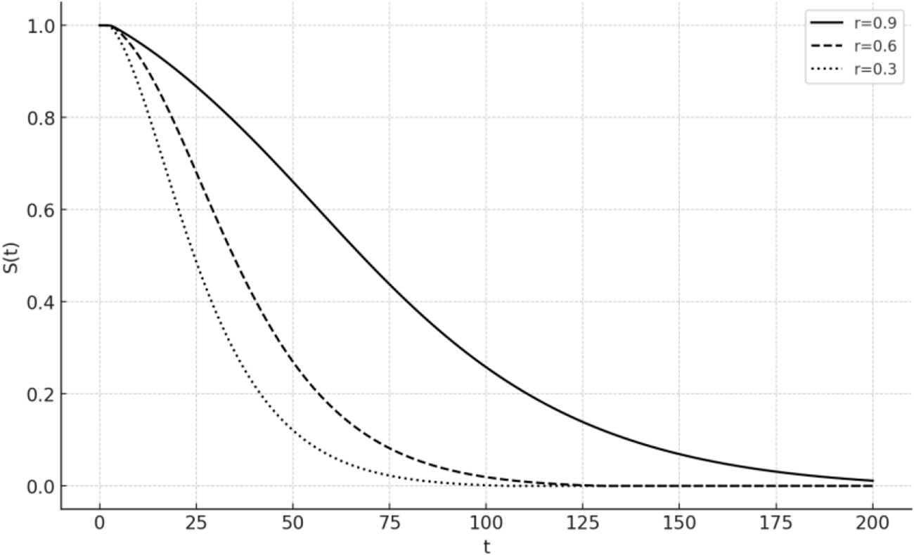
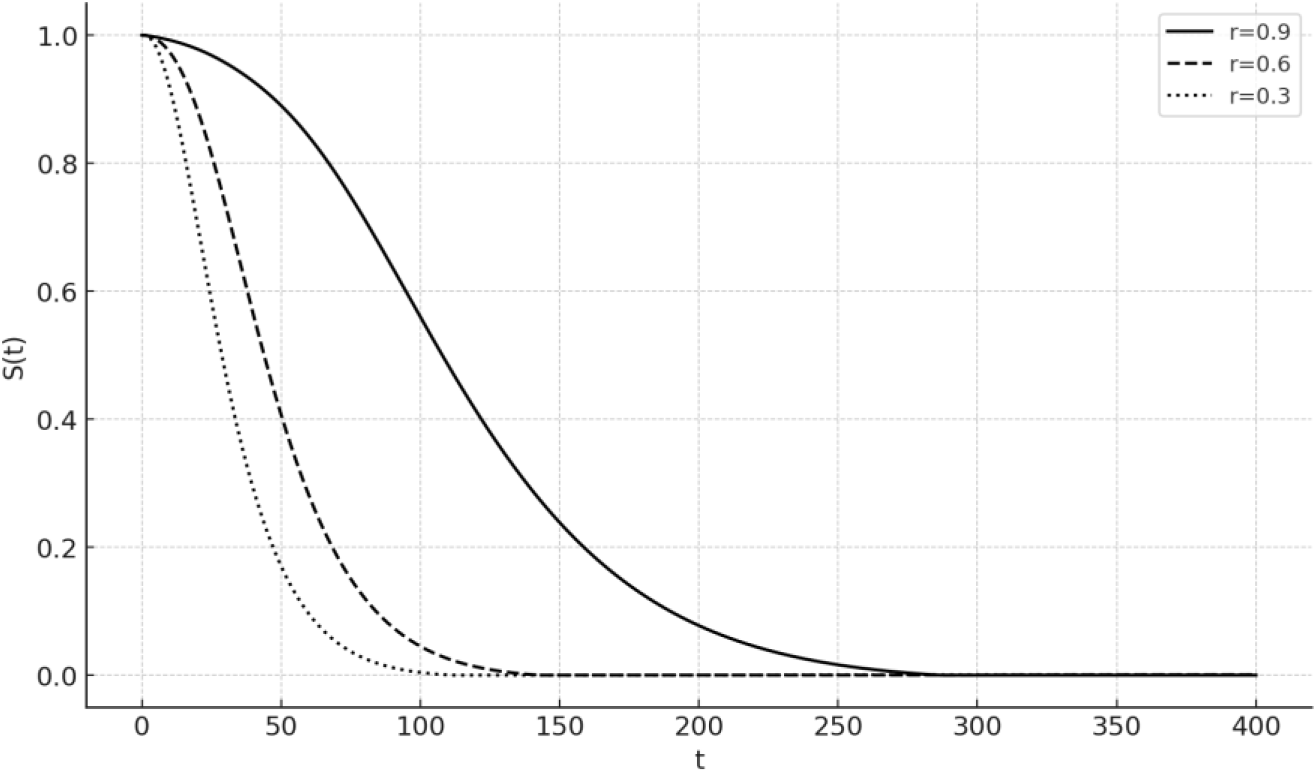
For the same values of  $\lambda = 0.1;{\text{ }}\mu = 1$ as in Figure 2 and
 $\delta = $2, 3, the plots for different values of
 $r = 0.9,{\text{ }}0.6,{\text{ }}0.3$ are given in Figures 3 and 4.
 $S( t )$ for
 $\lambda = 0.1;{\text{ }}\mu = 1$ and different values of
 $\delta $.

Survival curves for  $\delta = $2 and
 $\lambda = 0.1,{\text{ }}\mu = 1$.

Survival curves for  $\delta = $3 and
 $\lambda = 0.1,{\text{ }}\mu = 1$.

We see the obvious pattern of the curves, that is, with increase of  $\delta $, the “distance” between the corresponding curves is increasing.
4. Degrading repair times (Model 2)
We will now consider a sort of a dual setting to that in the previous section. Let, as in Section 2, the threshold  $\delta $ be fixed; however, the repair times are stochastically increasing with each repair also showing deterioration that can be interpreted as an imperfect repair. Thus,
 ${Y_i}$ are now independent but not identical random variables ordered as
 \begin{equation}{Y_1}{ \leq _{st}}{Y_2}{ \leq _{st}}{Y_3}{ \leq _{st}} \ldots ,{\text{ }}\end{equation}
where “st” denotes the usual stochastic ordering, that is,
 \begin{equation}{G_1}( t ) \geq {\text{ }}{G_2}( t ) \geq {\text{ }}{G_3}( t ) \geq \ldots \end{equation}
and  ${G_i}(t$) is the c.d.f. of the repair time of the ith consecutive defect. It follows from inequalities (15) that the means of these times are ordered accordingly and increase with i. Denote
 \begin{equation*}{q_n} = \Pr \left( {{Y_n} \gt {\text{ }}\delta } \right) = 1 - {G_n}\left( \delta \right),{\text{ }}n = 1,2, \ldots .\end{equation*}
As in the previous section,
 \begin{equation*}S(t) = \Pr \;(T \gt t);{S_n}(t) = \Pr \;({T_n} \gt t);S(t) \equiv {S_1}(t);{T_1} \equiv T,\end{equation*}
where  ${S_n}( t )$ is the survival probability of a system that starts (at t = 0) the nth cycle (thus, the previous ones were successful), whereas Tn is the corresponding lifetime, n = 1, 2, 3, … .
We will derive the integral equations for survival probabilities and will write them in a slightly more explicit form than in Eq. (11).
 \begin{equation}{S_n}( t ) = \bar F( t ) + \mathop \int \nolimits_0^t f\left( x \right)\mathop \int \nolimits_0^\delta {g_n}\left( y \right){S_{n + 1}}\left( {t - x - y} \right)\text{d}y\text{d}x + {q_n}\left( {F( t ) - F\left( {t - \delta } \right){\text{ }}} \right),{\text{ }}\end{equation}
where  ${g_n}( t )$ is the p.d.f. of
 ${Y_n}$. Probabilistic description of Eq. (16) is similar to that of Eq. (11). Indeed, the first term is the probability of no defect in
 $\left[ {0,t} \right)$, the second is the probability that the defect had occurred and was repaired during the time not exceeding
 $\delta $ and then a system starts the next cycle, whereas the last term is the probability that the defect had occurred in
 $\left[ {t - \delta ,t} \right)$ and it was not repaired in the rest of the interval.
We will now obtain the solution of this equation in an equivalent as previously way, but by direct reasoning in the “s” domain. In this case, it is more convenient to operate with the Laplace–Stieltjes transform (LST) of  ${T_n}$. Thus, denote the LST of
 ${T_n}$ as
 \begin{equation*}{L_n}\left( s \right) = E[\exp \left\{ { - s{T_n}} \right\}] = \mathop \int \nolimits_0^\infty \exp \left\{ { - sx} \right\}{f_n}\left( x \right)\text{d}x,\end{equation*}
where  ${f_n}( t )$ is the p.d.f. of
 ${T_n}$,
 ${f_1}( t ) \equiv f( t )$.
For the nth cycle, consider first the case when  ${Y_n} \gt \delta $, which means that this is the last cycle (FF). Then
 ${T_n} = {X_n} + \delta $ and
 \begin{equation}E\left[ {\exp \left\{ { - s({X_n} + \delta } \right\} \mathbf{1}\left\{ {{Y_n} \gt \delta } \right\}} \right] = {q_n}\exp \left\{ { - s\delta } \right\}\phi \left( s \right),{\text{ }}\end{equation}
where
 \begin{equation*}\phi \left( s \right) = E[\exp \left\{ { - s{X_n}} \right\}.\end{equation*}
Let now  ${Y_n} \leq \delta $, then
 ${T_n} = {X_n} + {Y_n} + {T_{n + 1}}$ and
 \begin{equation}E\left[ {\exp \left\{ { - s({X_n} + {Y_n} + {T_{n + 1}}} \right\}\mathbf{1}\left\{ {{Y_n} \leq \delta } \right\}} \right] = \phi \left( s \right){b_n}\left( s \right){L_{n + 1}}\left( s \right),{\text{ }}\end{equation}
where
 \begin{equation*}{b_n}\left( s \right) = E\left[ {\exp \left\{ { - s{Y_n}} \right\}{\mathbf{1}}\left\{ {{Y_n} \leq \delta } \right\}} \right] = \mathop {\int}\limits_{\delta} ^0 \exp \left\{ { - sy} \right\}{g_n}\left( y \right)\text{d}y.\end{equation*}
Combining Eqs. (17) and (18) results in
 \begin{equation}{L_n}\left( s \right) = \phi \left( s \right)\left[ {{q_n}\exp \left\{ { - s\delta } \right\} + {b_n}\left( s \right){L_{n + 1}}\left( s \right)} \right]{\text{ }}\end{equation}
Performing recursion starting with n = 1 and taking into account that  ${X_i} + {Y_i}$ are i.i.d.
 \begin{align}{L_1}\left( s \right) &= {\text{ }}\phi \left( s \right)\left[ {{q_1}\exp \left\{ { - s\delta } \right\} + {b_1}\left( s \right){L_2}\left( s \right)} \right]\nonumber\\ &= \phi \left( s \right){q_1}\exp \left\{ { - s\delta } \right\} + \phi \left( s \right){b_1}\left( s \right)\{ {\text{ }}\phi \left( s \right)\left[ {{q_2}\exp \left\{ { - s\delta } \right\} + {b_2}\left( s \right){L_3}\left( s \right)} \right] \phi \left( s \right){q_1}\exp \left\{ { - s\delta } \right\} \nonumber\\ &\quad + \phi {\left( s \right)^2}{b_1}\left( s \right){q_2}\exp \left\{ { - s\delta } \right\} + \phi {\left( s \right)^3}{b_1}\left( s \right){b_2}\left( s \right){q_3}\exp \left\{ { - s\delta } \right\} + \ldots {\text{ }}\end{align}
which results in the following compact form
 \begin{equation}{L_1}(s) = \exp \{ - s\delta \} \sum\limits_{n = 1}^\infty {\left( {\phi {{(s)}^n}{q_n}\prod\limits_{k = 1}^{n - 1} {{b_k}(S)} } \right)} \end{equation}
Loose interpretation of the  $n$th summand in the “s” domain:
 $\prod \nolimits_{k = 1}^{n - 1} {b_k}\left( s \right) - \left( {n - 1} \right){\text{ repairs were acceptable}}$ (i.e., were shorter than
 $\delta )$,
 ${q_n}$–the nth repair resulted in the FF,
 $\phi {\left( s \right)^n}$—there were n uptimes,
 $\exp \left\{ { - s\delta } \right\}$—the last repair contributed
 $\delta $ to the lifetime.
In accordance with our definitions, coming back to the LT
 \begin{align}{S^*}\left( s \right) \equiv S_1^*\left( s \right)& = \frac{{1 - {L_1}\left( s \right)}}{s}\nonumber\\ & = \frac{1}{s}\left[ {1 - \exp \left\{ { - s\delta } \right\}\mathop \sum \limits_{n = 1}^\infty \left( {\phi {{\left( s \right)}^n}{q_n}\mathop \prod \limits_{k = 1}^{n - 1} {b_k}\left( s \right)} \right){\text{ }}} \right]\end{align}
As in the previous section, consider a specific case of exponential distributions and geometrically increasing the mean of time to repair.
 \begin{equation*}\phi \left( s \right) = \frac{\lambda }{{\lambda + s}};{\text{ }}{q_n} = \exp \left\{ { - {\mu _n}\delta } \right\};{\text{ }}{\mu _n} = {\mu _0}{r^{n - 1}},n = 1,2, \ldots ,{\text{ }}r \lt 1,\end{equation*}
 \begin{equation*}{b_n}\left( s \right) = \mathop \int \nolimits_0^\delta {\mu _n}\exp \left\{ { - \left( {{\mu _n} + s} \right)y} \right\}\text{d} y = {\mu _n}\frac{{1 - {\text{exp}}\left\{ { - \left( {{\mu _n} + s} \right)\delta } \right\}}}{{{\mu _n} + s}}.\end{equation*}
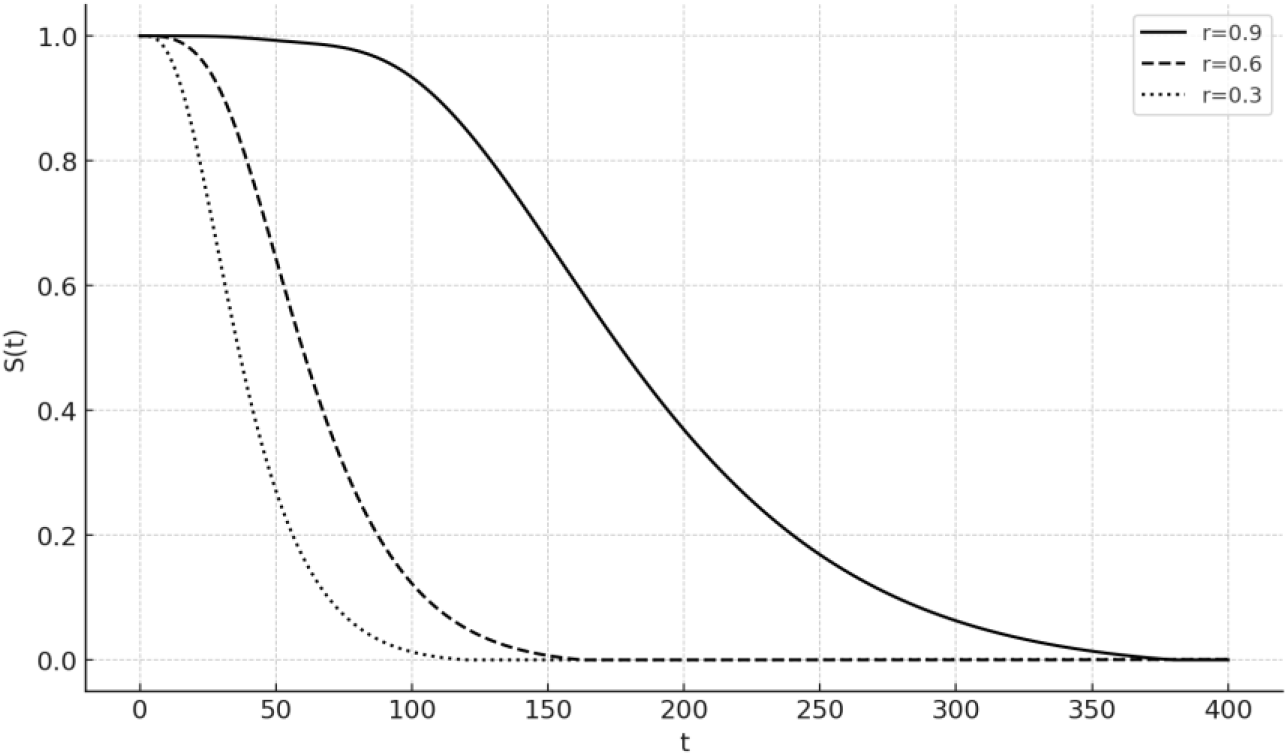
For illustration, let  $\lambda = 0.1;{\text{ }}{\mu _0} = 5$ and r = 0.9, 0.6 and 0.3. The corresponding plots are given in Figures 5 and 6.
Survival curves for  $\delta = $1 and
 $\lambda = 0.1,{\text{ }}{\mu _0} = 5$.

Survival curves for  $\delta = $2 and
 $\lambda = 0.1,{\text{ }}{\mu _0} = 5$.

As in the previous section, we see the obvious pattern of the curves, that is, with increase of  $\delta $, the “distance” between the corresponding curves is increasing. Moreover, when the coefficient of reduction r is close to 1 (0.9), the impact of the increase in
 $\delta $ is more noticeable than for smaller values of this parameter, which can be easily explained by the fact that in the latter case the FF occurs in both cases earlier in time.
5. Limited number of repairs
The number of repairs in the considered models can be limited [Reference Kurt and Kharoufeh18]. For example, due to the limited number of spares. On the other hand, as the quality of repair is degrading with each repair, it is also reasonable to stop operation of a system, to avoid losses from the FF, which probability is increasing with each successful cycle. Some practical examples for this limitation were also given in Section 1.
How shall we adjust Eq. (22) to account for the limited number of repairs? One cannot, obviously, just change the summation from infinity to this number. Denote it by N. If we have survived N successful repairs, we just then stop at  $\sum \nolimits_{k = 1}^N \left( {{X_k} + {Y_k}} \right)$ and our truncated recursion in Eq. (20) will result now in
 \begin{equation}L_1^{\left( N \right)}\left( s \right) = \exp \left\{ { - s\delta } \right\}\mathop \sum \limits_{n = 1}^N \left( {\phi {{\left( s \right)}^n}{q_n}\mathop \prod \limits_{k = 1}^{n - 1} {b_k}\left( s \right)} \right) + \phi {\left( s \right)^{}}{\text{ }}\mathop \prod \limits_{k = 1}^N {b_k}\left( s \right),{\text{ }}\end{equation}
where the last term accounts for the last cycle that was completed without failure. Then, as before
 \begin{equation}S_1^{*\left( N \right)}\left( s \right) = \frac{{1 - L_1^{\left( N \right)}\left( s \right)}}{s}{\text{ }}\end{equation}
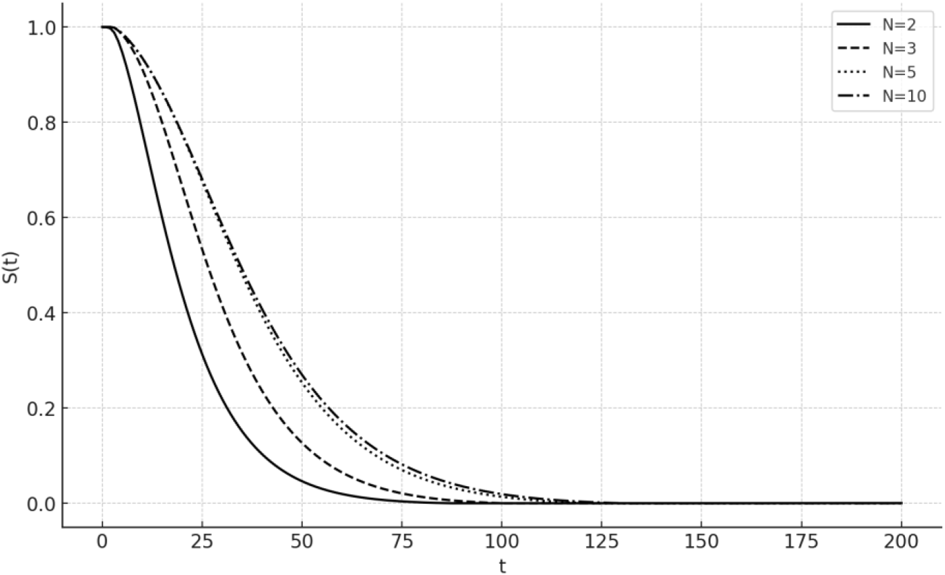
For illustration, as previously, let  $\lambda = 0.1;{\text{ }}{\mu _0} = 5$ and
 $\delta = $2
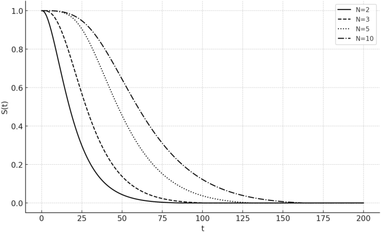
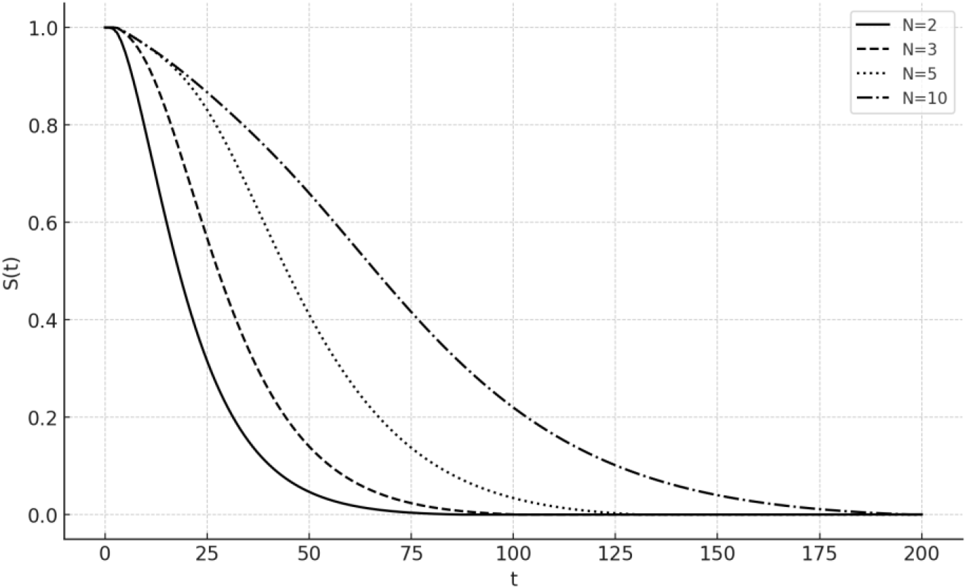
 $r = 0.9$, 0.6. Then the following curves are given for different values of N. We see that the effect of r is quite significant on the corresponding survival probabilities, whereas, as expected, these probabilities are increasing with increase of N. Moreover, for the chosen values of parameters in Figure 7, the curve that corresponds to N = 10 is very close to 1 up to t
 $ \approx $50. This is because
 ${q_n}$ is very small in this case and is increasing very slowly with n.
Model 2. Survival curves for r = 0.9 and  $\delta = $2,
 $\lambda = 0.1,{\text{ }}{\mu _0} = 5$.

We will also provide illustrations for Model 1 in Section 3 with decreasing redundancy thresholds and limited number of repairs. To do that in a uniform manner with Model 2 considered above, let us rewrite Eq. (13) in terms of the corresponding LST, similar to Eq. (21). It is easy to see that in this case (compare with Eq. (23))
 \begin{equation}L_1^{\left( N \right)}\left( s \right) = \mathop \sum \limits_{n = 1}^N \left( {\phi {{\left( s \right)}^n}{q_n}\exp \left\{ { - s{\delta _n}} \right\}\mathop \prod \limits_{k = 1}^{n - 1} {b_k}\left( s \right)} \right) + \phi {\left( s \right)^N}{\text{ }}\mathop \prod \limits_{k = 1}^N {b_k}\left( s \right),{\text{ }}\end{equation}
where for the specific exponential case:
 \begin{equation*}\phi \left( s \right) = \frac{\lambda }{{\lambda + s}};{\text{ }}{q_n} = \exp \left\{ { - \mu {r^{n - 1}}\delta } \right\} = {\text{exp}}\left\{ {\mu {\delta _n}} \right\}; n = 1,2, \ldots ,{\text{ }}r \lt 1\end{equation*}
 \begin{equation*}{b_n}\left( s \right) = \int \limits_0^{{\delta _n}} \exp \left\{ { - sy} \right\}g\left( y \right)\text{d}y = \mu \frac{{1 - {\text{exp}}\left\{ { - \left( {\mu + s} \right)} \right\}{\delta _n}}}{{\mu + s}}\end{equation*}
Thus,  ${q_n}$ and
 ${b_n}\left( s \right)$ are defined in slightly different way than for Model 2.
Comparing Figure 8 with Figure 9, we see that, as previously, the effect of r is quite significant on the corresponding survival probabilities. However, in Figure 9, distinct from Figure 10 for r = 0.6, we see that adding additional repairs (spares) beyond N = 5 practically does not increase the survival function. This means that due to the increased, as compared with r = 0.9, probability of failure at each stage, the expected number of successful cycles/stages will not be more than 5. This intuitive reasoning can be applied to other values of parameters as well.
Model 1. Survival curves for r = 0.9 and  $\delta = $3,
 $\lambda = 0.1,{\text{ }}\mu = 1$.

Model1. Survival curves for r = 0.6 and  $\delta = $3,
 $\lambda = 0.1,{\text{ }}\mu = 1$.

Model 2. Survival curves for r = 0.6,  $\delta = $1 and
 $\lambda = 0.1,{\text{ }}{\mu _0} = 5$.

6. Concluding remarks
We consider systems with final failures that occur when defects are not repaired in a timely manner. Therefore, operation of a system is described by the corresponding terminating renewal process. The FF occurs when the repair time exceeds some threshold for the first time. We use the corresponding renewal-type equations to derive relationships for the survival functions that describe times to failure of these systems.
We develop a general approach (based on integral equations) to obtaining and analyzing of reliability characteristics for the described settings, which allows for explicit general solutions in terms of LT. Note that LT approach is a standard technique; however, the corresponding analytical solutions are only possible where the transform can be inverted analytically. Apart from the baseline setting that is used as introduced in Section 2, we are the first to suggest and study more complex and often more relevant in practice new models:
Model 1. The distribution of time of repair is fixed but after each repair the period of inertia  ${\delta _i}$,
 $i = 1,2, \ldots $ is decreasing, that is,
 ${\delta _1} \gt {\delta _2}$, >
 ${\delta _3} \cdot \cdot \cdot $.
Model 2. The baseline  $\delta $ is fixed; however, the time of repair is stochastically decreasing with each repaired defect.
The results obtained can be further generalized in different ways. For instance,  $\delta $ itself can be random, which seems to be a natural generalization of the basic model. Due to deterioration, an optimal cost-wise maintenance problem can be considered when a system is replaced either on the FF or after the successful completion of the nth cycle. However, the latter needs further clarification and discussion in future research.
Acknowledgments
The author is grateful to two anonymous referees for extremely helpful comments and discussion.
Competing interest
The author declares that they have no known competing financial interests or personal relationships that could have appeared to influence the work reported in this paper.















 Open access

